Learning local Dirichlet-to-Neumann maps of nonlinear elliptic PDEs with rough coefficients

Miranda Boutilier miranda.boutilier@univ-cotedazur.fr Konstantin Brenner konstantin.brenner@univ-cotedazur.fr  and  Larissa Miguez lamiguez@posgrad.lncc.br
Abstract.

Partial differential equations (PDEs) involving high contrast and oscillating coefficients are common in scientific and industrial applications. Numerical approximation of these PDEs is a challenging task that can be addressed, for example, by multi-scale finite element analysis. For linear problems, multi-scale finite element method (MsFEM) is well established and some viable extensions to non-linear PDEs are known. However, some features of the method seem to be intrinsically based on linearity-based. In particular, traditional MsFEM rely on the reuse of computations. For example, the stiffness matrix can be calculated just once, while being used for several right-hand sides, or as part of a multi-level iterative algorithm. Roughly speaking, the offline phase of the method amounts to pre-assembling the local linear Dirichlet-to-Neumann (DtN) operators. We present some preliminary results concerning the combination of MsFEM with machine learning tools. The extension of MsFEM to nonlinear problems is achieved by means of learning local nonlinear DtN maps. The resulting learning-based multi-scale method is tested on a set of model nonlinear PDEs involving the plimit-from𝑝p-Laplacian and degenerate nonlinear diffusion.

The authors are presented in alphabetical order.

Introduction

A variety of real-world phenomena are described by Partial Differential Equations (PDEs). When solutions to PDE models present a high variability in small spatial regions or short periods of time, this behavior is considered multiscale. Standard numerical methods such as Finite Element, Finite Difference, or Finite Volume methods often have difficulty approximating multiscale behavior. Therefore, multiscale numerical methods have emerged as attractive options for dealing with such problems, including the Localized Orthogonal Decomposition method [16], Heterogeneous Multiscale methods [23], the Generalized Finite Element Method [1], the Multiscale Spectral Generalized Finite Element Method[2, 15] and the Multiscale Finite Element Method (MsFEM) [8]. MsFEM methods appear as a two-scale finite element approach: a macroscopic scale to capture the global solution behavior of the material and a microscopic scale to model fine heterogeneities. By integrating information from these two scales, MsFEM methods provide a more accurate solution for problems with multiscale behavior.

Furthermore, it is worth noting these methods offer the advantage of reusing calculations to enhance efficiency. For instance, the stiffness matrix of MsFEM can be computed once and reused multiple times, just as Domain Decomposition (DD) [6] techniques can benefit from the precomputation of LU decompositions of local matrices. However, MsFEM strategies do not naturally extend to nonlinear problems  [5, 7]; we focus therefore on the the computation of local Dirichlet-to-Neumann (DtN) operators. Specifically, with coarse (macroscopic) and fine (microscopic) partitionings of the heterogeneous domain, we can compute local DtN operators on each subdomain. These DtN local operators, to be defined in detail later, provide a relationship between Dirichlet and Neumann boundary data; these local operators lead to a nonlinear substructuring method such that the fine-scale discrete nonlinear problem can be written in terms of the local DtN maps.

On the other hand, with the renewed interest in Machine Learning (ML) within the scientific computing community, numerous techniques have been proposed to apply ML techniques to the solution of PDEs. In [14], the authors employ DeepONet neural networks to learn nonlinear operators. Additionally, the authors of [3] introduce an approach that combines Finite Element interpolation techniques with Neural Networks (NN) to solve a wide range of direct and inverse problems. Among these approaches are Physics-Informed Neural Networks (PINNs) [21]. The central idea behind PINNs is to minimize a functional representing the residual of the PDE and its initial and boundary conditions. Since then, many pieces of work have been published on PINNs, including [17, 4, 18]. However, problems with complex domains have led to other methodologies based on DD methods and PINNs, including Extended PINNs [10], Conservative PINNs [11], Variational PINNs [12] and Finite Basis Physics-Informed Neural Networks [19]. Additionally, [9] proposed Differential Machine Learning (DML), originally with a financial application. In DML, supervised learning is “extended” such that ML models are trained not only with values/inputs but also and on correpsonding derivatives.

In this work, we aim to use machine learning techniques to learn the local nonlinear DtN maps. The neural network is trained to replicate the action of the local nonlinear DtN maps on some coarse subset of the trace space. Once the training is completed, the surrogate DtN operators will be used to solve a nonlinear substructuring method, which is solved via Newton’s method. For training the nonlinear maps, we use an approach similar to DML; that is, we incorporate gradient information into the loss function. Additionally, we impose a monotonicity property into the loss function which is based on the known monotonicity of the DtN maps.

This paper is organized as follows. In Section 1, we introduce the model problem and associated approximate substructured formulation, which includes the definition of the continuous DtN maps. In Section 2, we introduce the finite element discretization, discrete substructured formulation, and discrete DtN maps. We also provide a description of the machine learning process which is used to determine the learned DtN operators and assemble the learned substructured formulation. Section 3 contains numerical experiments, showing both the accuracy of the learned DtN maps and the resulting learned approximate substructured formulation. Section 4 concludes with a summary and discussion for future work.

1. Model Problem and Approximate Substructured Problem

Let ΩΩ\Omega be either an open connected polygonal domain in 2superscript2\mathbb{R}^{2} or a real interval. In this work, we focus on model problems of the form

{au+div(Kϵ(𝐱)𝐅(u,u))=0inΩ,u=uDonΩ,cases𝑎𝑢divsubscript𝐾italic-ϵ𝐱𝐅𝑢𝑢0inΩ𝑢subscript𝑢𝐷onΩ\left\{\begin{array}[]{rll}au+\text{div}\left(K_{\epsilon}(\mathbf{x})\mathbf{F}(u,\nabla u)\right)&=&0\qquad\mbox{in}\qquad\Omega,\\ u&=&u_{D}\qquad\mbox{on}\qquad\partial\Omega,\\ \end{array}\right. (1)

where a𝑎a is a positive real coefficient and Kϵ(𝐱)subscript𝐾italic-ϵ𝐱K_{\epsilon}(\mathbf{x}), representing the heterogeneity of the problem, is assumed to satisfy Kϵ(𝐱)kmin>0subscript𝐾italic-ϵ𝐱subscript𝑘𝑚𝑖𝑛0K_{\epsilon}(\mathbf{x})\geq k_{min}>0 for all 𝐱Ω𝐱Ω{\bf x}\in\Omega. For the “flux functions” F(u,u)𝐹𝑢𝑢F(u,\nabla u), we consider either the model

F(u,u)=up,p>1,formulae-sequence𝐹𝑢𝑢superscript𝑢𝑝𝑝1F(u,\nabla u)=-\nabla u^{p},\quad p>1,

leading to a porous media problem, or the plimit-from𝑝p-Laplace model

F(u,u)=|u|pu,p>0.formulae-sequence𝐹𝑢𝑢superscript𝑢𝑝𝑢𝑝0F(u,\nabla u)=-|\nabla u|^{p}\nabla u,\quad p>0.

The well posedness of the problem (1) is known (see e.g. [22] and [13]).

1.1. Substructured and Approximate Substructured Problem

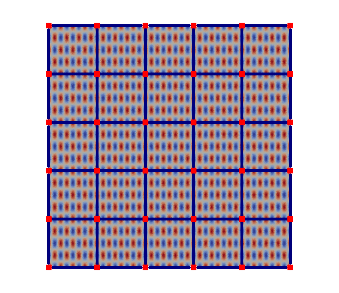
Consider a finite nonoverlapping rectangular partitioning of ΩΩ\Omega denoted by (Ωj)j=1NsuperscriptsubscriptsubscriptΩ𝑗𝑗1𝑁\left(\Omega_{j}\right)_{j=1}^{N}. We will refer to (Ωj)j=1NsuperscriptsubscriptsubscriptΩ𝑗𝑗1𝑁\left(\Omega_{j}\right)_{j=1}^{N} as the coarse mesh over ΩΩ\Omega. Additionally, we denote by ΓΓ\Gamma its skeleton, that is Γ=j=1NΩjΓsuperscriptsubscript𝑗1𝑁subscriptΩ𝑗\Gamma=\bigcup_{j=1}^{N}\partial\Omega_{j}. With this, each edge of the skeleton ΓΓ\Gamma is denoted by Γij=ΩiΩjsubscriptΓ𝑖𝑗subscriptΩ𝑖subscriptΩ𝑗\Gamma_{ij}=\partial\Omega_{i}\cap\partial\Omega_{j}, while the set of the coarse grid nodes is defined by {𝔰α}α=1𝒩Γ=i,j=1NΓijsuperscriptsubscriptsubscript𝔰𝛼𝛼1subscript𝒩Γsuperscriptsubscript𝑖𝑗1𝑁subscriptΓ𝑖𝑗\{\mathfrak{s}_{\alpha}\}_{\alpha=1}^{\mathscr{N}_{\Gamma}}=\bigcup_{i,j=1}^{N}\partial\Gamma_{ij}. An example of the coarse partitioning and corresponding coarse grid nodes is shown in Figure 1.
Refer to caption
Figure 1. Heterogeneous domain Kϵ(𝐱)subscript𝐾italic-ϵ𝐱K_{\epsilon}(\mathbf{x}) with N=5×5𝑁55N=5\times 5 coarse cells. Nonoverlapping skeleton ΓΓ\Gamma is denoted by thick dark blue lines.

The Dirichlet-to-Neumann (DtN) map provides a mathematical relationship between Dirichlet and Neumann boundary data, allowing us to compute one set of boundary data from the other, which can be very useful in solving boundary value problems. Given a nonoverlapping partitioning of domain, these DtN maps can be defined and computed locally on each subdomain. Let us consider a local Dirichlet problem

{aui+div(Kϵ(𝐱)𝐅(ui,ui))=0inΩi,ui=gionΩi.cases𝑎subscript𝑢𝑖divsubscript𝐾italic-ϵ𝐱𝐅subscript𝑢𝑖subscript𝑢𝑖0insubscriptΩ𝑖subscript𝑢𝑖subscript𝑔𝑖onsubscriptΩ𝑖\left\{\begin{array}[]{rll}au_{i}+\text{div}\left(K_{\epsilon}(\mathbf{x})\mathbf{F}(u_{i},\nabla u_{i})\right)&=&0\qquad\mbox{in}\qquad\Omega_{i},\\ \displaystyle u_{i}&=&g_{i}\qquad\mbox{on}\quad\partial\Omega_{i}.\end{array}\right. (2)

For a given gisubscript𝑔𝑖g_{i} we formally denote by DtNi(gi)subscriptDtN𝑖subscript𝑔𝑖{\rm DtN}_{i}(g_{i}) the the Neumann traces of uisubscript𝑢𝑖u_{i} on ΩisubscriptΩ𝑖\partial{\Omega_{i}}, that is

DtNi(gi)=Kϵ(𝐱)𝐅(ui,ui)|Ωi𝐧ionΩi,subscriptDtN𝑖subscript𝑔𝑖evaluated-atsubscript𝐾italic-ϵ𝐱𝐅subscript𝑢𝑖subscript𝑢𝑖subscriptΩ𝑖subscript𝐧𝑖onsubscriptΩ𝑖{\rm DtN}_{i}(g_{i})=K_{\epsilon}(\mathbf{x})\mathbf{F}(u_{i},\nabla u_{i})|_{\partial\Omega_{i}}\cdot\mathbf{n}_{i}\qquad\text{on}\quad\partial{\Omega_{i}},

where 𝐧isubscript𝐧𝑖\mathbf{n}_{i} denotes the unit outward normal on ΩisubscriptΩ𝑖\partial{\Omega_{i}}.

Our main idea with the nonlinear substructuring method is to replace the original problem (1) by the one which only involves the unknown Dirichlet data g𝑔g defined over ΓΓ\Gamma. This new unknown function is determined by imposing a matching flux condition along the edges of the skeleton ΓΓ\Gamma.

For a regular enough function g𝑔g defined on ΓΓ\Gamma, we formally introduce the local jump operator, returning the mismatch in fluxes on a given coarse edge

ij:gDtNi(g|Ωi)|Γij+DtNi(g|Ωj)|Γij.\llbracket\rrbracket_{ij}:g\mapsto{\rm DtN}_{i}(g|_{\partial\Omega_{i}})|_{\Gamma_{ij}}+{\rm DtN}_{i}(g|_{\partial\Omega_{j}})|_{\Gamma_{ij}}.

and the global jump operator \llbracket\rrbracket is given by g|Γij=gij\llbracket g\rrbracket|_{\Gamma_{ij}}=\llbracket g\rrbracket_{ij}. Enforcing zero flux jump at every coarse edge ΓijsubscriptΓ𝑖𝑗\Gamma_{ij}, leads to a global substructured problem that can be written in a weak form as: find g𝑔g satisfying g|Ω=uDevaluated-at𝑔Ωsubscript𝑢𝐷g|_{\partial\Omega}=u_{D} such that for all regular enough w𝑤w vanishing on ΩΩ\partial\Omega it holds that

Γgwdγ(𝐱)=0.\displaystyle\int_{\Gamma}\llbracket g\rrbracket w\,d\gamma({\bf x})=0. (3)

Let us assume for the moment that we are in the possession of a procedure allowing to compute evaluate the DtN operators. Then, the problem (3) can be discretized by taking the test and trial function from a finite dimensional space. In particular, we consider the space VH(Γ)subscript𝑉𝐻ΓV_{H}(\Gamma) made of the continuous functions on ΓΓ\Gamma that are affine on every coarse edge of ΓΓ\Gamma, that is

VH(Γ)={vC0(Γ)s.t.v|Γij1(Γij) for all Γij}.subscript𝑉𝐻Γformulae-sequence𝑣superscript𝐶0Γs.t.evaluated-at𝑣subscriptΓ𝑖𝑗subscript1subscriptΓ𝑖𝑗 for all subscriptΓ𝑖𝑗V_{H}(\Gamma)=\{v\in C^{0}(\Gamma)\quad\text{s.t.}\quad v|_{\Gamma_{ij}}\in\mathbb{P}_{1}(\Gamma_{ij})\quad\text{ for all }\quad\Gamma_{ij}\}. (4)

Let VH,0(Γ)={vVH(Γ)s.t.v|Ω=0}subscript𝑉𝐻0Γformulae-sequence𝑣subscript𝑉𝐻Γs.t.evaluated-at𝑣Ω0V_{H,0}(\Gamma)=\{v\in V_{H}(\Gamma)\quad\text{s.t.}\quad v|_{\partial{\Omega}}=0\} and let uD,HVH(Γ)subscript𝑢𝐷𝐻subscript𝑉𝐻Γu_{D,H}\in V_{H}(\Gamma) denote some approximation of uDsubscript𝑢𝐷u_{D}, e.g. obtained by interpolation. To form the approximate substructured problem in VH(Γ)subscript𝑉𝐻ΓV_{H}(\Gamma), one then replaces the problem (3) by: find gHsubscript𝑔𝐻g_{H} satisfying gH|Ω=uH,Devaluated-atsubscript𝑔𝐻Ωsubscript𝑢𝐻𝐷g_{H}|_{\partial\Omega}=u_{H,D} and

ΓgHwHdγ(𝐱)=0wHVH,0(Γ).\displaystyle\int_{\Gamma}\llbracket g_{H}\rrbracket w_{H}\,d\gamma({\bf x})=0\qquad\forall w_{H}\in V_{H,0}(\Gamma). (5)

2. Discrete Finite Element Substructuring and DtN Maps

2.1. Finite element discretization and domain decomposition

Let Thsubscript𝑇{T}_{h} denote the triangulation of ΩΩ\Omega which is supposed to be conforming with respect to partitioning (Ωj)j=1NsuperscriptsubscriptsubscriptΩ𝑗𝑗1𝑁\left(\Omega_{j}\right)_{j=1}^{N}. Let {sk}k=1Ω¯superscriptsubscriptsubscript𝑠𝑘𝑘1¯Ω\{s_{k}\}_{k=1}^{\overline{\Omega}} be the set of vertices (or points) of Thsubscript𝑇{T}_{h}. We introduce the finite element space defined by

Vh={v|vC0(Ω¯),s.t.v|t1,for alltTh},subscript𝑉conditional-set𝑣formulae-sequence𝑣superscript𝐶0¯Ωs.t.formulae-sequenceevaluated-at𝑣𝑡subscript1for all𝑡subscript𝑇V_{h}=\{v\,\,|\,\,v\in C^{0}(\overline{\Omega}),\quad\text{s.t.}\quad v|_{t}\in\mathbb{P}_{1},\quad\text{for all}\quad t\in{T}_{h}\},

and we denote the corresponding nodal “hat” basis functions (ηk)k=1NΩsuperscriptsubscriptsuperscript𝜂𝑘𝑘1subscript𝑁Ω(\eta^{k})_{k=1}^{N_{\Omega}} for each point in sksubscript𝑠𝑘s_{k}. Let Vh,0=VhH01subscript𝑉0subscript𝑉superscriptsubscript𝐻01V_{h,0}=V_{h}\cap H_{0}^{1}, and let uh,DVhsubscript𝑢𝐷subscript𝑉u_{h,D}\in V_{h} be some approximation of the boundary data uDsubscript𝑢𝐷u_{D}. The Galerkin finite element formulation is as follows:

Find uhVh satisfying uh|Ω=uh,D such thatΩauhvh(Kϵ(𝐱)𝐅(uh,uh))vhd𝐱=0for allvhVh,0.Find uhVh satisfying uh|Ω=uh,D such thatmissing-subexpressionmissing-subexpressionmissing-subexpressionmissing-subexpressionformulae-sequencesubscriptΩ𝑎subscript𝑢subscript𝑣subscript𝐾italic-ϵ𝐱𝐅subscript𝑢subscript𝑢subscript𝑣𝑑𝐱0for allsubscript𝑣subscript𝑉0missing-subexpressionmissing-subexpressionmissing-subexpressionmissing-subexpression\begin{array}[]{lllll}\text{Find $u_{h}\in V_{h}$ satisfying $u_{h}|_{\Omega}=u_{h,D}$ such that}\\[2.0pt] \displaystyle\int_{\Omega}\,au_{h}v_{h}-(K_{\epsilon}(\mathbf{x})\mathbf{F}(u_{h},\nabla u_{h}))\cdot\nabla v_{h}\,d{\bf x}=0\qquad\text{for all}\quad v_{h}\in V_{h,0}.\end{array} (6)

Now, consider the following linear reconstruction operator πhsubscript𝜋\pi_{h} acting from NΩsuperscriptsubscript𝑁Ω\mathbb{R}^{N_{\Omega}} to Vhsubscript𝑉V_{h}, such that

πh(v)(𝐱)=k=1NΩvkηk(𝐱).subscript𝜋𝑣𝐱superscriptsubscript𝑘1subscript𝑁Ωsuperscript𝑣𝑘superscript𝜂𝑘𝐱\displaystyle\pi_{h}(v)({\bf x})=\sum_{k=1}^{N_{\Omega}}v^{k}\eta^{k}({\bf x}).

We note that πhsubscript𝜋\pi_{h} is bijective, with (π1(𝐯h))k=vh(sk)superscriptsuperscript𝜋1subscript𝐯𝑘subscript𝑣subscript𝑠𝑘\left(\pi^{-1}({\bf v}_{h})\right)^{k}=v_{h}(s_{k}) for any triangulation point sksubscript𝑠𝑘s_{k}.

We denote by F𝐹F the “Neumann residual” function corresponding to (6); more precisely F𝐹F acts from NΩsuperscriptsubscript𝑁Ω\mathbb{R}^{N_{\Omega}} to itself and has its l𝑙lth component defined by

(F(u))l=Ωπh(u)ηlKϵ(𝐱)𝐅(πh(u),πh(u))ηld𝐱,superscript𝐹𝑢𝑙subscriptΩsubscript𝜋𝑢superscript𝜂𝑙subscript𝐾italic-ϵ𝐱𝐅subscript𝜋𝑢subscript𝜋𝑢superscript𝜂𝑙𝑑𝐱\left(F(u)\right)^{l}=\int_{\Omega}\pi_{h}(u)\,\eta^{l}-K_{\epsilon}(\mathbf{x})\mathbf{F}(\pi_{h}(u),\nabla\pi_{h}(u))\cdot\nabla\eta^{l}\,d{\bf x}, (7)

for l=1,,NΩ𝑙1subscript𝑁Ωl=1,\ldots,N_{\Omega}.

Before moving any further, let us introduce some notation related to the decomposition of the mesh and finite element degrees of freedom induced by the partitioning (Ωi)i=1NsubscriptsuperscriptsubscriptΩ𝑖𝑁𝑖1\left({\Omega_{i}}\right)^{N}_{i=1} of ΩΩ\Omega. Let J={1,,NΩ¯}𝐽1subscript𝑁¯ΩJ=\{1,\ldots,N_{\overline{\Omega}}\} denote the index set of the triangulation points, for any ωΩ¯𝜔¯Ω\omega\in\overline{\Omega} we introduce a subset of indices

Jω={jω1,jωNω}Jsubscript𝐽𝜔superscriptsubscript𝑗𝜔1superscriptsubscript𝑗𝜔subscript𝑁𝜔𝐽J_{\omega}=\left\{j_{\omega}^{1},\ldots j_{\omega}^{N_{\omega}}\right\}\subset J

such that jJω𝑗subscript𝐽𝜔j\in J_{\omega} if and only if the point sjsubscript𝑠𝑗s_{j} belongs to ω𝜔\omega. We note that the number of elements in Jωsubscript𝐽𝜔J_{\omega} is denoted by Nωsubscript𝑁𝜔N_{\omega}.

The standard Nωsubscript𝑁𝜔N_{\omega} by NΩ¯subscript𝑁¯ΩN_{\overline{\Omega}} boolean restriction matrix 𝐑ωsubscript𝐑𝜔\mathbf{R}_{\omega} “from Ω¯¯Ω\overline{\Omega} to ω𝜔\omega” is defined by

(𝐑ω)kl={1ifl=jωk,0else,subscriptsubscript𝐑𝜔𝑘𝑙cases1if𝑙superscriptsubscript𝑗𝜔𝑘missing-subexpressionmissing-subexpressionmissing-subexpression0else,missing-subexpressionmissing-subexpressionmissing-subexpression\left(\mathbf{R}_{\omega}\right)_{kl}=\left\{\begin{array}[]{lllll}1&\text{if}\quad l=j_{\omega}^{k},\\ 0&\text{else,}\end{array}\right.

for any k=1,,Nω𝑘1subscript𝑁𝜔k=1,\ldots,N_{\omega} and l=1,,NΩ¯𝑙1subscript𝑁¯Ωl=1,\ldots,N_{\overline{\Omega}}. Further, for any A,BΩ¯𝐴𝐵¯ΩA,B\subset\overline{\Omega}, we denote 𝐑BA=𝐑A(𝐑B)Tsubscriptsuperscript𝐑𝐴𝐵subscript𝐑𝐴superscriptsubscript𝐑𝐵𝑇\mathbf{R}^{A}_{B}=\mathbf{R}_{A}(\mathbf{R}_{B})^{T}. If AB𝐴𝐵A\subset B the matrix 𝐑BAsubscriptsuperscript𝐑𝐴𝐵\mathbf{R}^{A}_{B} can be interpreted as a restriction matrix “from B𝐵B to A𝐴A”. Conversely, if BA𝐵𝐴B\subset A, the same 𝐑BAsubscriptsuperscript𝐑𝐴𝐵\mathbf{R}^{A}_{B} may be interpreted as an extension matrix “from B𝐵B to A𝐴A”. Let us mention a couple of useful properties of this restriction/extension linear operator. First, we note that for any C𝐶C such that A,BCΩ¯𝐴𝐵𝐶¯ΩA,B\subset C\subset\overline{\Omega} we have

𝐑CA𝐑BC=𝐑BA=𝐑ABA𝐑BAB.subscriptsuperscript𝐑𝐴𝐶subscriptsuperscript𝐑𝐶𝐵subscriptsuperscript𝐑𝐴𝐵subscriptsuperscript𝐑𝐴𝐴𝐵subscriptsuperscript𝐑𝐴𝐵𝐵\mathbf{R}^{A}_{C}\mathbf{R}^{C}_{B}=\mathbf{R}^{A}_{B}=\mathbf{R}^{A}_{A\cap B}\mathbf{R}^{A\cap B}_{B}.

With this, the discrete problem (6) can be expressed as follows:

Find uNΩ such that 𝐑Ωu=𝐑Ωπh1(uh,D) and satisfying𝐑ΩF(u)=0.Find uNΩ such that 𝐑Ωu=𝐑Ωπh1(uh,D) and satisfyingsubscript𝐑Ω𝐹𝑢0missing-subexpressionmissing-subexpressionmissing-subexpression\begin{array}[]{llll}\text{Find $u\in\mathbb{R}^{N_{\Omega}}$ such that $\mathbf{R}_{\partial\Omega}u=\mathbf{R}_{\partial\Omega}\pi_{h}^{-1}\left(u_{h,D}\right)$ and satisfying}\,\,\mathbf{R}_{\Omega}F(u)=0.\end{array} (8)

We note that the integral in (6) can be split into a sum of integrals over ΩisubscriptΩ𝑖{\Omega_{i}}, meaning that the finite element residual can be assembled by gluing together some the local contributions. We detail below this local assembly procedure because of it use for the substructured formulation.

For a subdomain ΩisubscriptΩ𝑖{\Omega_{i}} let {ηil}l=1NΩ¯isuperscriptsubscriptsuperscriptsubscript𝜂𝑖𝑙𝑙1subscript𝑁subscript¯Ω𝑖\{\eta_{i}^{l}\}_{l=1}^{N_{{\overline{\Omega}_{i}}}} denote the set of local finite element basis functions such that ηil(𝐱)=ηjΩ¯il(𝐱)|Ωisuperscriptsubscript𝜂𝑖𝑙𝐱evaluated-atsuperscript𝜂superscriptsubscript𝑗subscript¯Ω𝑖𝑙𝐱subscriptΩ𝑖\eta_{i}^{l}({\bf x})=\eta^{j_{\overline{\Omega}_{i}}^{l}}({\bf x})|_{\Omega_{i}} for all l=1,,NΩ¯i𝑙1subscript𝑁subscript¯Ω𝑖l=1,\ldots,N_{{\overline{\Omega}_{i}}}. The local function reconstruction operator πh,isubscript𝜋𝑖\pi_{h,i} is defined by πhi(vi)(𝐱)=l=1NΩ¯ivlηil(𝐱)subscript𝜋subscript𝑖subscript𝑣𝑖𝐱superscriptsubscript𝑙1subscript𝑁subscript¯Ω𝑖superscript𝑣𝑙superscriptsubscript𝜂𝑖𝑙𝐱\displaystyle\pi_{h_{i}}(v_{i})({\bf x})=\sum_{l=1}^{N_{{\overline{\Omega}_{i}}}}v^{l}\eta_{i}^{l}({\bf x}). Similar to (7) we define the local residual functions Fisubscript𝐹𝑖F_{i}. That is for any uiNΩ¯isubscript𝑢𝑖superscriptsubscript𝑁subscript¯Ω𝑖u_{i}\in\mathbb{R}^{N_{\overline{\Omega}_{i}}} and l=1,,NΩ¯i𝑙1subscript𝑁subscript¯Ω𝑖l=1,\ldots,N_{\overline{\Omega}_{i}}, we set

(Fi(ui))l=Ωiπh,i(u)ηilKϵ(𝐱)𝐅(πh,i(ui),πh,i(ui))ηild𝐱.superscriptsubscript𝐹𝑖subscript𝑢𝑖𝑙subscriptsubscriptΩ𝑖subscript𝜋𝑖𝑢subscriptsuperscript𝜂𝑙𝑖subscript𝐾italic-ϵ𝐱𝐅subscript𝜋𝑖subscript𝑢𝑖subscript𝜋𝑖subscript𝑢𝑖subscriptsuperscript𝜂𝑙𝑖𝑑𝐱\left(F_{i}(u_{i})\right)^{l}=\int_{\Omega_{i}}\pi_{h,i}(u)\,\eta^{l}_{i}-K_{\epsilon}(\mathbf{x})\mathbf{F}(\pi_{h,i}(u_{i}),\nabla\pi_{h,i}(u_{i}))\cdot\nabla\eta^{l}_{i}\,d{\bf x}. (9)

with ηil=ηjΩ¯ilsuperscriptsubscript𝜂𝑖𝑙superscript𝜂superscriptsubscript𝑗subscript¯Ω𝑖𝑙\eta_{i}^{l}=\eta^{j_{\overline{\Omega}_{i}}^{l}}. For any uNΩ¯𝑢superscriptsubscript𝑁¯Ωu\in\mathbb{R}^{N_{\overline{\Omega}}} the global residual F(u)𝐹𝑢F(u) is obtained from the local components by the following expression

F(u)=i=1N𝐑Ω¯iTFi(𝐑Ω¯iu).𝐹𝑢superscriptsubscript𝑖1𝑁superscriptsubscript𝐑subscript¯Ω𝑖𝑇subscript𝐹𝑖subscript𝐑subscript¯Ω𝑖𝑢F(u)=\sum_{i=1}^{N}\mathbf{R}_{{\overline{\Omega}_{i}}}^{T}F_{i}(\mathbf{R}_{\overline{\Omega}_{i}}u). (10)

.

2.2. Discrete DtNDtN{\rm DtN} maps

In this section we introduce the finite element version the Dirichlet-to-Neumann operator, associated with our model PDE and a subdomain ΩisubscriptΩ𝑖{\Omega_{i}}. This discrete operator, denoted by DtNh,isubscriptDtN𝑖{\rm DtN}_{h,i}, is defined as the nonlinear mapping from the set of degrees of freedom NΩisuperscriptsubscript𝑁subscriptΩ𝑖\mathbb{R}^{N_{\partial\Omega_{i}}} associated with the boundary of ΩisubscriptΩ𝑖{\Omega_{i}} to itself. We also provides the formula for the (Fréchet) derivative of DtNh,isubscriptDtN𝑖{\rm DtN}_{h,i}. The construction of DtNh,isubscriptDtN𝑖{\rm DtN}_{h,i} relies on the definition (9) of the local “Neumann” residual Fisubscript𝐹𝑖F_{i}.

Let us split the set of induces JΩ¯isubscript𝐽subscript¯Ω𝑖J_{{\overline{\Omega}_{i}}} into two non-overlapping subsets JΩisubscript𝐽subscriptΩ𝑖J_{\Omega_{i}} and JΩisubscript𝐽subscriptΩ𝑖J_{\partial{\Omega_{i}}} associated with internal degrees of freedom located in ΩisubscriptΩ𝑖\Omega_{i} and on the boundary ΩisubscriptΩ𝑖\partial\Omega_{i}. This gives the representation of the vector uiNΩ¯isubscript𝑢𝑖superscriptsubscript𝑁subscript¯Ω𝑖u_{i}\in\mathbb{R}^{N_{{\overline{\Omega}_{i}}}} associated to the subdomain Ω¯isubscript¯Ω𝑖{\overline{\Omega}_{i}} in the form ui=𝐑ΩiΩ¯iuΩi+𝐑ΩiΩ¯iuΩisubscript𝑢𝑖superscriptsubscript𝐑subscriptΩ𝑖subscript¯Ω𝑖subscript𝑢subscriptΩ𝑖superscriptsubscript𝐑subscriptΩ𝑖subscript¯Ω𝑖subscript𝑢subscriptΩ𝑖u_{i}=\mathbf{R}_{{\Omega_{i}}}^{{\overline{\Omega}_{i}}}u_{\Omega_{i}}+\mathbf{R}_{\partial{\Omega_{i}}}^{{\overline{\Omega}_{i}}}u_{\partial\Omega_{i}} with some uΩiNΩisubscript𝑢subscriptΩ𝑖superscriptsubscript𝑁subscriptΩ𝑖u_{\Omega_{i}}\in\mathbb{R}^{N_{\Omega_{i}}} and uΩiNΩisubscript𝑢subscriptΩ𝑖superscriptsubscript𝑁subscriptΩ𝑖u_{\partial{\Omega_{i}}}\in\mathbb{R}^{N_{\partial{\Omega_{i}}}}. In turn, we express the local Neumann residual as following

Fi(ui)=𝐑ΩiΩ¯iFΩi(uΩi,uΩi)+𝐑ΩiΩ¯iFΩi(uΩi,uΩi)subscript𝐹𝑖subscript𝑢𝑖superscriptsubscript𝐑subscriptΩ𝑖subscript¯Ω𝑖subscript𝐹subscriptΩ𝑖subscript𝑢subscriptΩ𝑖subscript𝑢subscriptΩ𝑖superscriptsubscript𝐑subscriptΩ𝑖subscript¯Ω𝑖subscript𝐹subscriptΩ𝑖subscript𝑢subscriptΩ𝑖subscript𝑢subscriptΩ𝑖F_{i}(u_{i})=\mathbf{R}_{{\Omega_{i}}}^{\overline{\Omega}_{i}}F_{\Omega_{i}}(u_{\Omega_{i}},u_{\partial\Omega_{i}})+\mathbf{R}_{\partial{\Omega_{i}}}^{\overline{\Omega}_{i}}F_{\partial{\Omega_{i}}}(u_{\Omega_{i}},u_{\partial\Omega_{i}}) (11)

where

FΩi(uΩi,uΩi)=𝐑Ω¯iΩiFi(𝐑ΩiΩ¯iuΩi+𝐑ΩiΩ¯iuΩi)subscript𝐹subscriptΩ𝑖subscript𝑢subscriptΩ𝑖subscript𝑢subscriptΩ𝑖superscriptsubscript𝐑subscript¯Ω𝑖subscriptΩ𝑖subscript𝐹𝑖superscriptsubscript𝐑subscriptΩ𝑖subscript¯Ω𝑖subscript𝑢subscriptΩ𝑖superscriptsubscript𝐑subscriptΩ𝑖subscript¯Ω𝑖subscript𝑢subscriptΩ𝑖F_{\Omega_{i}}(u_{\Omega_{i}},u_{\partial\Omega_{i}})=\mathbf{R}_{{\overline{\Omega}_{i}}}^{{\Omega_{i}}}F_{i}\left(\mathbf{R}_{{\Omega_{i}}}^{{\overline{\Omega}_{i}}}u_{\Omega_{i}}+\mathbf{R}_{\partial{\Omega_{i}}}^{{\overline{\Omega}_{i}}}u_{\partial\Omega_{i}}\right)

and

FΩi(uΩi,uΩi)=𝐑Ω¯iΩiFi(𝐑ΩiΩ¯iuΩi+𝐑ΩiΩ¯iuΩi).subscript𝐹subscriptΩ𝑖subscript𝑢subscriptΩ𝑖subscript𝑢subscriptΩ𝑖superscriptsubscript𝐑subscript¯Ω𝑖subscriptΩ𝑖subscript𝐹𝑖superscriptsubscript𝐑subscriptΩ𝑖subscript¯Ω𝑖subscript𝑢subscriptΩ𝑖superscriptsubscript𝐑subscriptΩ𝑖subscript¯Ω𝑖subscript𝑢subscriptΩ𝑖F_{\partial\Omega_{i}}(u_{\Omega_{i}},u_{\partial\Omega_{i}})=\mathbf{R}_{{\overline{\Omega}_{i}}}^{\partial{\Omega_{i}}}F_{i}\left(\mathbf{R}_{{\Omega_{i}}}^{{\overline{\Omega}_{i}}}u_{\Omega_{i}}+\mathbf{R}_{\partial{\Omega_{i}}}^{{\overline{\Omega}_{i}}}u_{\partial\Omega_{i}}\right).

The discrete counterpart of the local Dirichlet problem (2) can be expressed as:

Find uΩi such thatFΩi(uΩi,gΩi)=0Find uΩi such thatsubscript𝐹subscriptΩ𝑖subscript𝑢subscriptΩ𝑖subscript𝑔subscriptΩ𝑖0\text{Find $u_{\Omega_{i}}$ such that}\,\,F_{\Omega_{i}}(u_{\Omega_{i}},g_{\partial{\Omega_{i}}})=0 (12)

for a given gΩiNΩisubscript𝑔subscriptΩ𝑖superscriptsubscript𝑁subscriptΩ𝑖g_{\partial{\Omega_{i}}}\in\mathbb{R}^{N_{\partial{\Omega_{i}}}}. Assuming that (12) admits unique solution for any gΩisubscript𝑔subscriptΩ𝑖g_{\partial{\Omega_{i}}}, we define the solution operator GΩisubscript𝐺subscriptΩ𝑖G_{{\Omega_{i}}} from NΩisuperscriptsubscript𝑁subscriptΩ𝑖\mathbb{R}^{N_{\partial{\Omega_{i}}}} to NΩisuperscriptsubscript𝑁subscriptΩ𝑖\mathbb{R}^{N_{{\Omega_{i}}}} such that

FΩi(GΩi(gΩi),gΩi)=0subscript𝐹subscriptΩ𝑖subscript𝐺subscriptΩ𝑖subscript𝑔subscriptΩ𝑖subscript𝑔subscriptΩ𝑖0F_{{\Omega_{i}}}\left(G_{{\Omega_{i}}}(g_{\partial{\Omega_{i}}}),g_{\partial{\Omega_{i}}}\right)=0 (13)

for all gΩisubscript𝑔subscriptΩ𝑖g_{\partial{\Omega_{i}}}. With that, the discrete DtN operator is defined by

DtNh,i(gΩi)=FΩi(GΩi(gΩi),gΩi).subscriptDtN𝑖subscript𝑔subscriptΩ𝑖subscript𝐹subscriptΩ𝑖subscript𝐺subscriptΩ𝑖subscript𝑔subscriptΩ𝑖subscript𝑔subscriptΩ𝑖{\rm DtN}_{h,i}(g_{\partial{\Omega_{i}}})=F_{\partial{\Omega_{i}}}\left(G_{{\Omega_{i}}}(g_{\partial{\Omega_{i}}}),g_{\partial{\Omega_{i}}}\right). (14)

Under the assumptions of Implicit Function Theorem (see e.g. Proposition 5.2.4. of [20]) the Fréchet derivative of DtNh,isubscriptDtN𝑖{\rm DtN}_{h,i} can be expressed as

DtNh,i(uΩi)superscriptsubscriptDtN𝑖subscript𝑢subscriptΩ𝑖\displaystyle{\rm DtN}_{h,i}^{\prime}(u_{\partial\Omega_{i}}) =ΩiFΩi(GΩi(uΩi),uΩi)GΩi(uΩi)+ΩiFΩi(GΩi(uΩi),uΩi).absentsubscriptsubscriptΩ𝑖subscript𝐹subscriptΩ𝑖subscript𝐺subscriptΩ𝑖subscript𝑢subscriptΩ𝑖subscript𝑢subscriptΩ𝑖subscriptsuperscript𝐺subscriptΩ𝑖subscript𝑢subscriptΩ𝑖subscriptsubscriptΩ𝑖subscript𝐹subscriptΩ𝑖subscript𝐺subscriptΩ𝑖subscript𝑢subscriptΩ𝑖subscript𝑢subscriptΩ𝑖\displaystyle=\partial_{\Omega_{i}}F_{\partial\Omega_{i}}(G_{\Omega_{i}}(u_{\partial\Omega_{i}}),u_{\partial\Omega_{i}})G^{\prime}_{\Omega_{i}}(u_{\partial\Omega_{i}})+\partial_{\partial\Omega_{i}}F_{\partial\Omega_{i}}(G_{\Omega_{i}}(u_{\partial\Omega_{i}}),u_{\partial\Omega_{i}}). (15)

Recalling that uΩi=GΩi(uΩi)subscript𝑢subscriptΩ𝑖subscript𝐺subscriptΩ𝑖subscript𝑢subscriptΩ𝑖u_{\Omega_{i}}=G_{\Omega_{i}}(u_{\partial\Omega_{i}}), we have

DtNh,i(uΩi)superscriptsubscriptDtN𝑖subscript𝑢subscriptΩ𝑖\displaystyle{\rm DtN}_{h,i}^{\prime}(u_{\partial\Omega_{i}}) =ΩiFΩi(uΩi,uΩi)GΩi(uΩi)+ΩiFΩi(uΩi,uΩi),absentsubscriptsubscriptΩ𝑖subscript𝐹subscriptΩ𝑖subscript𝑢subscriptΩ𝑖subscript𝑢subscriptΩ𝑖subscriptsuperscript𝐺subscriptΩ𝑖subscript𝑢subscriptΩ𝑖subscriptsubscriptΩ𝑖subscript𝐹subscriptΩ𝑖subscript𝑢subscriptΩ𝑖subscript𝑢subscriptΩ𝑖\displaystyle=\partial_{\Omega_{i}}F_{\partial\Omega_{i}}(u_{\Omega_{i}},u_{\partial\Omega_{i}})G^{\prime}_{\Omega_{i}}(u_{\partial\Omega_{i}})+\partial_{\partial\Omega_{i}}F_{\partial\Omega_{i}}(u_{\Omega_{i}},u_{\partial\Omega_{i}}), (16)

where, thanks to the identity

FΩi(GΩi(uΩi),uΩi)=0,subscript𝐹subscriptΩ𝑖subscript𝐺subscriptΩ𝑖subscript𝑢subscriptΩ𝑖subscript𝑢subscriptΩ𝑖0F_{\Omega_{i}}(G_{\Omega_{i}}(u_{\partial\Omega_{i}}),u_{\partial\Omega_{i}})=0, (17)

we have

GΩi(uΩi)subscriptsuperscript𝐺subscriptΩ𝑖subscript𝑢subscriptΩ𝑖\displaystyle G^{\prime}_{\Omega_{i}}(u_{\partial\Omega_{i}}) =(ΩiFΩi(uΩi,uΩi))1Ωi(FΩi(uΩi,uΩi)).absentsuperscriptsubscriptsubscriptΩ𝑖subscript𝐹subscriptΩ𝑖subscript𝑢subscriptΩ𝑖subscript𝑢subscriptΩ𝑖1subscriptsubscriptΩ𝑖subscript𝐹subscriptΩ𝑖subscript𝑢subscriptΩ𝑖subscript𝑢subscriptΩ𝑖\displaystyle=-\left(\partial_{\Omega_{i}}F_{\Omega_{i}}(u_{\Omega_{i}},u_{\partial\Omega_{i}})\right)^{-1}\partial_{\partial\Omega_{i}}\left(F_{\Omega_{i}}(u_{\Omega_{i}},u_{\partial\Omega_{i}})\right). (18)

Plugging (18) into (15) results in

DtNh,i(uΩi)superscriptsubscriptDtN𝑖subscript𝑢subscriptΩ𝑖\displaystyle{\rm DtN}_{h,i}^{\prime}(u_{\partial\Omega_{i}}) =ΩiFΩi(uΩi,uΩi)(ΩiFΩi(uΩi,uΩi))1ΩiFΩi(uΩi,uΩi)+ΩiFΩi(uΩi,uΩi),absentsubscriptsubscriptΩ𝑖subscript𝐹subscriptΩ𝑖subscript𝑢subscriptΩ𝑖subscript𝑢subscriptΩ𝑖superscriptsubscriptsubscriptΩ𝑖subscript𝐹subscriptΩ𝑖subscript𝑢subscriptΩ𝑖subscript𝑢subscriptΩ𝑖1subscriptsubscriptΩ𝑖subscript𝐹subscriptΩ𝑖subscript𝑢subscriptΩ𝑖subscript𝑢subscriptΩ𝑖subscriptsubscriptΩ𝑖subscript𝐹subscriptΩ𝑖subscript𝑢subscriptΩ𝑖subscript𝑢subscriptΩ𝑖\displaystyle=-\partial_{\Omega_{i}}F_{\partial\Omega_{i}}(u_{\Omega_{i}},u_{\partial\Omega_{i}})\left(\partial_{\Omega_{i}}F_{\Omega_{i}}(u_{\Omega_{i}},u_{\partial\Omega_{i}})\right)^{-1}\partial_{\partial\Omega_{i}}F_{\Omega_{i}}(u_{\Omega_{i}},u_{\partial\Omega_{i}})+\partial_{\partial\Omega_{i}}F_{\partial\Omega_{i}}(u_{\Omega_{i}},u_{\partial\Omega_{i}}),

We remark that computing uΩisubscript𝑢subscriptΩ𝑖u_{\Omega_{i}} requires solving the local nonlinear problem (12) with uΩisubscript𝑢subscriptΩ𝑖u_{\partial\Omega_{i}} as data. This is typically done my some fixed point method. Ones the approximate value of uΩisubscript𝑢subscriptΩ𝑖u_{\Omega_{i}} is obtained, computing DtNh,i(uΩi)superscriptsubscriptDtN𝑖subscript𝑢subscriptΩ𝑖{\rm DtN}_{h,i}^{\prime}(u_{\partial\Omega_{i}}) requires solving the linear system with matrix right-hand-sides given by FΩi(uΩi,uΩi)subscript𝐹subscriptΩ𝑖subscript𝑢subscriptΩ𝑖subscript𝑢subscriptΩ𝑖F_{\Omega_{i}}(u_{\Omega_{i}},u_{\partial\Omega_{i}}). If uΩisubscript𝑢subscriptΩ𝑖u_{\Omega_{i}} is obtained by exact Newton’s method, the former can be done at marginal computational cost.

2.3. Discrete Substructured Problems

With DtNh,isubscriptDtN𝑖{\rm DtN}_{h,i} introduced above, let us provide the substructured formulation of the discrete problem (8). Let gNΓ𝑔superscriptsubscript𝑁Γg\in\mathbb{R}^{N_{\Gamma}} be a vector representing the unknown solution values at the skeleton ΓΓ\Gamma. Denoting gΩi=𝐑ΓΩigsubscript𝑔subscriptΩ𝑖subscriptsuperscript𝐑subscriptΩ𝑖Γ𝑔g_{\partial{\Omega_{i}}}=\mathbf{R}^{\partial{\Omega_{i}}}_{\Gamma}g and ui=GΩi(gΩi)subscript𝑢𝑖subscript𝐺subscriptΩ𝑖subscript𝑔subscriptΩ𝑖u_{i}=G_{\Omega_{i}}\left(g_{\partial{\Omega_{i}}}\right), we express the unknown discrete solution as

u=𝐑ΓTg+i=1N𝐑ΩiTuΩi.𝑢superscriptsubscript𝐑Γ𝑇𝑔superscriptsubscript𝑖1𝑁superscriptsubscript𝐑subscriptΩ𝑖𝑇subscript𝑢subscriptΩ𝑖u=\mathbf{R}_{\Gamma}^{T}g+\sum_{i=1}^{N}\mathbf{R}_{\Omega_{i}}^{T}u_{\Omega_{i}}. (19)

Observing that 𝐑Ω¯iu=𝐑ΩiΩ¯igΩi+𝐑ΩiΩ¯iuΩisubscript𝐑subscript¯Ω𝑖𝑢subscriptsuperscript𝐑subscript¯Ω𝑖subscriptΩ𝑖subscript𝑔subscriptΩ𝑖subscriptsuperscript𝐑subscript¯Ω𝑖subscriptΩ𝑖subscript𝑢subscriptΩ𝑖\mathbf{R}_{{\overline{\Omega}_{i}}}u=\mathbf{R}^{\overline{\Omega}_{i}}_{\partial{\Omega_{i}}}g_{\partial{\Omega_{i}}}+\mathbf{R}^{\overline{\Omega}_{i}}_{\Omega_{i}}u_{\Omega_{i}}, in view of (11), we deduce that

Fi(𝐑Ω¯iu)=𝐑ΩiΩ¯iFΩi(uΩi,gΩi)+𝐑ΩiΩ¯iFΩi(uΩi,gΩi).subscript𝐹𝑖subscript𝐑subscript¯Ω𝑖𝑢superscriptsubscript𝐑subscriptΩ𝑖subscript¯Ω𝑖subscript𝐹subscriptΩ𝑖subscript𝑢subscriptΩ𝑖subscript𝑔subscriptΩ𝑖superscriptsubscript𝐑subscriptΩ𝑖subscript¯Ω𝑖subscript𝐹subscriptΩ𝑖subscript𝑢subscriptΩ𝑖subscript𝑔subscriptΩ𝑖F_{i}\left(\mathbf{R}_{{\overline{\Omega}_{i}}}u\right)=\mathbf{R}_{{\Omega_{i}}}^{\overline{\Omega}_{i}}F_{\Omega_{i}}(u_{\Omega_{i}},g_{\partial{\Omega_{i}}})+\mathbf{R}_{\partial{\Omega_{i}}}^{\overline{\Omega}_{i}}F_{\partial{\Omega_{i}}}(u_{\Omega_{i}},g_{\partial{\Omega_{i}}}). (20)

The first term in the right hand side of (20) is zero by definition of uΩisubscript𝑢subscriptΩ𝑖u_{\Omega_{i}}, which yields

F(u)=i=1N𝐑ΩiTDtNh,i(gΩi)=i=1N𝐑ΩiTDtNh,i(𝐑ΓΩig),𝐹𝑢superscriptsubscript𝑖1𝑁superscriptsubscript𝐑subscriptΩ𝑖𝑇subscriptDtN𝑖subscript𝑔subscriptΩ𝑖superscriptsubscript𝑖1𝑁superscriptsubscript𝐑subscriptΩ𝑖𝑇subscriptDtN𝑖subscriptsuperscript𝐑subscriptΩ𝑖Γ𝑔F(u)=\sum_{i=1}^{N}\mathbf{R}_{\partial{\Omega_{i}}}^{T}{\rm DtN}_{h,i}\left(g_{\partial{\Omega_{i}}}\right)=\sum_{i=1}^{N}\mathbf{R}_{\partial{\Omega_{i}}}^{T}{\rm DtN}_{h,i}\left(\mathbf{R}^{\partial{\Omega_{i}}}_{\Gamma}g\right),

in view of (10) and (14). Let us denote

FΓ(g)=i=1N𝐑ΩiΓDtNh,i(𝐑ΓΩig).subscript𝐹Γ𝑔superscriptsubscript𝑖1𝑁subscriptsuperscript𝐑ΓsubscriptΩ𝑖subscriptDtN𝑖subscriptsuperscript𝐑subscriptΩ𝑖Γ𝑔F_{\Gamma}(g)=\sum_{i=1}^{N}\mathbf{R}^{\Gamma}_{\partial{\Omega_{i}}}{\rm DtN}_{h,i}\left(\mathbf{R}^{\partial{\Omega_{i}}}_{\Gamma}g\right). (21)

Substituting F(u)=𝐑ΓTFΓ(g)𝐹𝑢superscriptsubscript𝐑Γ𝑇subscript𝐹Γ𝑔F(u)=\mathbf{R}_{\Gamma}^{T}F_{\Gamma}(g) in (8) leads to the equation 𝐑Ω𝐑ΓFΓ(g)=0subscript𝐑Ωsubscript𝐑Γsubscript𝐹Γ𝑔0\mathbf{R}_{\Omega}\mathbf{R}_{\Gamma}F_{\Gamma}(g)=0. Since the latter is trivially satisfied for all degrees of freedom not lying on ΓΓ\Gamma, the system has to be reduced to ΓΩΓΩ\Gamma\cap\Omega, leading to

0=𝐑ΩΓΩ𝐑Ω𝐑ΓFΓ(g)=𝐑ΓΓΩFΓ(g).0subscriptsuperscript𝐑ΓΩΩsubscript𝐑Ωsubscript𝐑Γsubscript𝐹Γ𝑔subscriptsuperscript𝐑ΓΩΓsubscript𝐹Γ𝑔0=\mathbf{R}^{\Gamma\cap\Omega}_{\Omega}\mathbf{R}_{\Omega}\mathbf{R}_{\Gamma}F_{\Gamma}(g)=\mathbf{R}^{\Gamma\cap\Omega}_{\Gamma}F_{\Gamma}(g).

We have obtain the following substructured problem: find gNΓ𝑔superscriptsubscript𝑁Γg\in\mathbb{R}^{N_{\Gamma}} such that 𝐑ΓΩg=𝐑Ωπh1(uh,D)subscriptsuperscript𝐑ΩΓ𝑔subscript𝐑Ωsuperscriptsubscript𝜋1subscript𝑢𝐷\mathbf{R}^{\partial\Omega}_{\Gamma}g=\mathbf{R}_{\partial\Omega}\pi_{h}^{-1}(u_{h,D}) and

𝐑ΩΓΩFΓ(g)=0.subscriptsuperscript𝐑ΓΩΩsubscript𝐹Γ𝑔0\mathbf{R}^{\Gamma\cap\Omega}_{\Omega}F_{\Gamma}(g)=0. (22)

2.4. Coarse discrete DtNDtN{\rm DtN} maps and discrete approximate substructuring

We now proceed to the discrete version of the approximate substructured problem (5). Similar to the definitions introduced in Section 2.1, for any ωΓ𝜔Γ\omega\subset\Gamma, we denote by 𝒩ωsubscript𝒩𝜔\mathscr{N}_{\omega} the number of coarse nodes belonging to ω𝜔\omega, and by Γωsubscriptsuperscript𝜔Γ\mathscr{R}^{\omega}_{\Gamma} the restriction matrix from the 𝒩Γsuperscriptsubscript𝒩Γ\mathbb{R}^{\mathscr{N}_{\Gamma}} to 𝒩ωsuperscriptsubscript𝒩𝜔\mathbb{R}^{\mathscr{N}_{\omega}}. As before, the transpose of Γωsubscriptsuperscript𝜔Γ\mathscr{R}^{\omega}_{\Gamma} is denoted by ωΓsuperscriptsubscript𝜔Γ\mathscr{R}_{\omega}^{\Gamma}.

Let (ϕα)α=1𝒩Γsuperscriptsubscriptsuperscriptitalic-ϕ𝛼𝛼1subscript𝒩Γ(\phi^{\alpha})_{\alpha=1}^{\mathscr{N}_{\Gamma}} be a nodal basis of VH(Γ)subscript𝑉𝐻ΓV_{H}(\Gamma) made of “hat” functions associated to the set coarse grid nodes {𝔰α}α=1𝒩Γsuperscriptsubscriptsubscript𝔰𝛼𝛼1subscript𝒩Γ\{\mathfrak{s}_{\alpha}\}_{\alpha=1}^{\mathscr{N}_{\Gamma}} (see Figure 1 for visual). More precisely, the basis function ϕαVH(Γ)superscriptitalic-ϕ𝛼subscript𝑉𝐻Γ\phi^{\alpha}\in V_{H}(\Gamma) is assumed to satisfy

ϕα(𝔰j)={1,α=j,0,αj,superscriptitalic-ϕ𝛼subscript𝔰𝑗cases1𝛼𝑗0𝛼𝑗\phi^{\alpha}(\mathfrak{s}_{j})=\begin{cases}1,&\alpha=j,\\ 0,&\alpha\neq j,\\ \end{cases}

for all coarse grid nodes 𝔰jsubscript𝔰𝑗\mathfrak{s}_{j}. Given this nodal basis in VH(Γ)subscript𝑉𝐻ΓV_{H}(\Gamma) we define the function reconstruction operator πHsubscript𝜋𝐻\pi_{H} from 𝒩Γsuperscriptsubscript𝒩Γ\mathbb{R}^{\mathscr{N}_{\Gamma}} to VH(Γ)subscript𝑉𝐻ΓV_{H}(\Gamma) by πH(v)(𝐱)=α=1𝒩Γvαϕα(𝐱)subscript𝜋𝐻𝑣𝐱superscriptsubscript𝛼1subscript𝒩Γsuperscript𝑣𝛼superscriptitalic-ϕ𝛼𝐱\displaystyle\pi_{H}(v)({\bf x})=\sum_{\alpha=1}^{\mathscr{N}_{\Gamma}}v^{\alpha}\phi^{\alpha}({\bf x}). We further denote by 𝚽Hsubscript𝚽𝐻{\boldsymbol{\Phi}}_{H} the NΓsubscript𝑁ΓN_{\Gamma} by 𝒩Γsubscript𝒩Γ\mathscr{N}_{\Gamma} matrix whose columns contains the values of the basis functions ϕαsuperscriptitalic-ϕ𝛼\phi^{\alpha} at the skeletal degrees of freedom; more specifically, the j𝑗jth component of a column index α𝛼\alpha of 𝚽Hsubscript𝚽𝐻{\boldsymbol{\Phi}}_{H} is given by

(𝚽H)j,α=ϕα(sjΓj).superscriptsubscript𝚽𝐻𝑗𝛼superscriptitalic-ϕ𝛼subscript𝑠superscriptsubscript𝑗Γ𝑗({\boldsymbol{\Phi}}_{H})^{j,\alpha}=\phi^{\alpha}(s_{j_{\Gamma}^{j}}).

for α=1,,𝒩Γ𝛼1subscript𝒩Γ\alpha=1,\ldots,\mathscr{N}_{\Gamma} and each j=1,,NΓ𝑗1subscript𝑁Γj=1,\ldots,N_{\Gamma}.

The local version of 𝚽Hsubscript𝚽𝐻{\boldsymbol{\Phi}}_{H} is defined by

𝚽Hi=𝐑ΓΩi𝚽HΩiΓ,subscript𝚽𝐻𝑖superscriptsubscript𝐑ΓsubscriptΩ𝑖subscript𝚽𝐻superscriptsubscriptsubscriptΩ𝑖Γ{\boldsymbol{\Phi}}_{Hi}=\mathbf{R}_{\Gamma}^{\partial\Omega_{i}}{\boldsymbol{\Phi}}_{H}\mathscr{R}_{\partial{\Omega_{i}}}^{\Gamma}, (23)

where 𝚽Hisubscript𝚽𝐻𝑖{\boldsymbol{\Phi}}_{Hi} is composed of the 𝒩Ωisubscript𝒩subscriptΩ𝑖\mathscr{N}_{\partial{\Omega_{i}}} local basis vectors of size NΩisubscript𝑁subscriptΩ𝑖N_{\partial\Omega_{i}} corresponding to the local coarse grid nodes on ΩisubscriptΩ𝑖\partial\Omega_{i}. We note that 𝚽Hisubscript𝚽𝐻𝑖{\boldsymbol{\Phi}}_{Hi} satisfies

𝐑ΓΩi𝚽H=𝚽HiΓΩi.superscriptsubscript𝐑ΓsubscriptΩ𝑖subscript𝚽𝐻subscript𝚽𝐻𝑖subscriptsuperscriptsubscriptΩ𝑖Γ\mathbf{R}_{\Gamma}^{\partial\Omega_{i}}{\boldsymbol{\Phi}}_{H}={\boldsymbol{\Phi}}_{Hi}\mathscr{R}^{\partial{\Omega_{i}}}_{\Gamma}. (24)

In order to derive the coarse approximation of the problem (22) we first express the latter in the following variational form:

Find g such that 𝐑ΓΩg=𝐑Ωπh1(uh,D) and satisfyingvTFΓ(g)=0for allvIm(𝐑ΓΩΓ).Find g such that 𝐑ΓΩg=𝐑Ωπh1(uh,D) and satisfyingmissing-subexpressionmissing-subexpressionmissing-subexpressionformulae-sequencesuperscript𝑣𝑇subscript𝐹Γ𝑔0for all𝑣Imsuperscriptsubscript𝐑ΓΩΓmissing-subexpressionmissing-subexpressionmissing-subexpression\begin{array}[]{llll}\text{Find $g$ such that $\mathbf{R}_{\Gamma}^{\partial\Omega}g=\mathbf{R}_{\partial\Omega}\pi_{h}^{-1}(u_{h,D})$ and satisfying}\\[7.0pt] \displaystyle v^{T}\,F_{\Gamma}(g)=0\qquad\text{for all}\quad v\in{\rm Im}\left(\mathbf{R}_{\Gamma\cap\Omega}^{\Gamma}\right).\end{array} (25)

The Galerkin approximation of (25) using the coarse space VH(Γ)subscript𝑉𝐻ΓV_{H}(\Gamma) is obtained by setting g𝚽HgH𝑔subscript𝚽𝐻subscript𝑔𝐻g\approx{\boldsymbol{\Phi}}_{H}g_{H} with some appropriate boundary conditions and taking the test elements v𝑣v in Im(𝐑ΓΩΓ)Im(𝚽H)=Im(𝚽H)Im(ΓΩΓ)Imsuperscriptsubscript𝐑ΓΩΓImsubscript𝚽HImsubscript𝚽HImsuperscriptsubscriptΓΩΓ{\rm Im}\left(\mathbf{R}_{\Gamma\cap\Omega}^{\Gamma}\right)\cap{\rm Im\left({\boldsymbol{\Phi}}_{H}\right)}={\rm Im\left({\boldsymbol{\Phi}}_{H}\right)}\cap{\rm Im}\left(\mathscr{R}_{\Gamma\cap\Omega}^{\Gamma}\right). The latter amount to set v=𝚽HΓΩΓ𝐯H𝑣subscript𝚽𝐻superscriptsubscriptΓΩΓsubscript𝐯𝐻v={\boldsymbol{\Phi}}_{H}\mathscr{R}_{\Gamma\cap\Omega}^{\Gamma}{\bf v}_{H} with vH𝔑ΓΩsubscript𝑣𝐻superscriptsubscript𝔑ΓΩv_{H}\in\mathbb{R}^{\mathfrak{N}_{\Gamma\cap\Omega}}. This leads to the system

ΓΓΩ𝚽HTFΓ(𝚽HgH)=0.subscriptsuperscriptΓΩΓsuperscriptsubscript𝚽𝐻𝑇subscript𝐹Γsubscript𝚽𝐻subscript𝑔𝐻0\mathscr{R}^{\Gamma\cap\Omega}_{\Gamma}{\boldsymbol{\Phi}}_{H}^{T}F_{\Gamma}\left({\boldsymbol{\Phi}}_{H}g_{H}\right)=0.

In view of (21) and (24), we have

i=1N𝚽HT𝐑ΩiΓDtNh,i(𝐑ΓΩi𝚽HTgH)=i=1NΩiΓ𝚽HiTDtNh,i(𝚽HiΓΩigH).superscriptsubscript𝑖1𝑁superscriptsubscript𝚽𝐻𝑇subscriptsuperscript𝐑ΓsubscriptΩ𝑖subscriptDtN𝑖subscriptsuperscript𝐑subscriptΩ𝑖Γsuperscriptsubscript𝚽𝐻𝑇subscript𝑔𝐻superscriptsubscript𝑖1𝑁superscriptsubscriptsubscriptΩ𝑖Γsuperscriptsubscript𝚽𝐻𝑖𝑇subscriptDtN𝑖subscript𝚽𝐻𝑖subscriptsuperscriptsubscriptΩ𝑖Γsubscript𝑔𝐻\sum_{i=1}^{N}{\boldsymbol{\Phi}}_{H}^{T}\mathbf{R}^{\Gamma}_{\partial{\Omega_{i}}}{\rm DtN}_{h,i}\left(\mathbf{R}^{\partial{\Omega_{i}}}_{\Gamma}{\boldsymbol{\Phi}}_{H}^{T}g_{H}\right)=\sum_{i=1}^{N}\mathscr{R}_{\partial{\Omega_{i}}}^{\Gamma}{\boldsymbol{\Phi}}_{Hi}^{T}{\rm DtN}_{h,i}\left({\boldsymbol{\Phi}}_{Hi}\mathscr{R}^{\partial{\Omega_{i}}}_{\Gamma}g_{H}\right).

With this, the definition of the coarse DtNDtN{\rm DtN} operator acting from 𝒩Ωisuperscriptsubscript𝒩subscriptΩ𝑖\mathbb{R}^{\mathscr{N}_{\partial{\Omega_{i}}}} to itself given by

DtNH,i=𝚽HiTDtNh,i𝚽Hi,subscriptDtN𝐻𝑖superscriptsubscript𝚽𝐻𝑖𝑇subscriptDtN𝑖subscript𝚽𝐻𝑖{\rm DtN}_{H,i}={\boldsymbol{\Phi}}_{Hi}^{T}\circ{\rm DtN}_{h,i}\circ{\boldsymbol{\Phi}}_{Hi}, (26)

such that we denote

FH(gH)=i=1NΩiΓDtNH,i(ΓΩigH).subscript𝐹𝐻subscript𝑔𝐻superscriptsubscript𝑖1𝑁superscriptsubscriptsubscriptΩ𝑖ΓsubscriptDtN𝐻𝑖subscriptsuperscriptsubscriptΩ𝑖Γsubscript𝑔𝐻F_{H}(g_{H})=\sum_{i=1}^{N}\mathscr{R}_{\partial{\Omega_{i}}}^{\Gamma}{\rm DtN}_{H,i}(\mathscr{R}^{\partial{\Omega_{i}}}_{\Gamma}g_{H}). (27)

Let uH,DVH(Γ)subscript𝑢𝐻𝐷subscript𝑉𝐻Γu_{H,D}\in V_{H}(\Gamma) be some approximation of uDsubscript𝑢𝐷u_{D}, the coarse Galerkin approximation of (8), or equivalently, the finite element approximation of (5) reads as follows:

Find gH𝒩Γ such that ΓΩgH=ΓΩπH1(uH,D) andΓΓΩFH(gH)=0.Find gH𝒩Γ such that ΓΩgH=ΓΩπH1(uH,D) andsuperscriptsubscriptΓΓΩsubscript𝐹𝐻subscript𝑔𝐻0missing-subexpressionmissing-subexpressionmissing-subexpression\begin{array}[]{llll}\text{Find $g_{H}\in\mathbb{R}^{\mathscr{N}_{\Gamma}}$ such that $\mathscr{R}_{\Gamma}^{\partial\Omega}g_{H}=\mathscr{R}_{\Gamma}^{\partial\Omega}\pi_{H}^{-1}(u_{H,D})$ and}\,\,\mathscr{R}_{\Gamma}^{\Gamma\cap\Omega}F_{H}(g_{H})=0.\end{array} (28)

We remark that even though it is considered a coarse approximation, the computation of the discrete DtNisubscriptDtN𝑖\text{DtN}_{i} relies on fine-scale information and fine-scale input. That is, it still takes in as input a vector of size NΓsubscript𝑁ΓN_{\Gamma} which lives on the fine degrees of freedom along the skeleton ΓΓ\Gamma. This computation can still become quite expensive and the cost is not to be negated, as DtNisubscriptDtN𝑖\text{DtN}_{i} must be computed at each Newton iteration used to solve the discrete substructured problem.

2.5. Learning Dirichlet-to-Neumann maps

In Section 2, we discussed the computation of the DtN map and how by nature, the substructured problem results in the DtN map being computed at each Newton iteration. As this computation can get very expensive, we explore a Scientific Machine Learning (SciML) application to our problem. Specifically, we introduce learned local DtN operators which we denote as DtN~H,isubscript~DtN𝐻𝑖\widetilde{\text{DtN}}_{H,i}.Once the model is generated, we can call the model at each Newton iteration without the need for a separate computation on each subdomain. We remark that if the heterogeneities are periodic in each subdomain, we can use the same NN model.

Let DtN~H,isubscript~DtN𝐻𝑖\widetilde{\text{DtN}}_{H,i} denote some approximation of DtNH,isubscriptDtN𝐻𝑖\text{DtN}_{H,i} to which we will refere to as to a surrogate model, and which is going to be introduced in more details below. By replacing in (27) the original operator DtNH,isubscriptDtN𝐻𝑖\text{DtN}_{H,i} by DtN~H,isubscript~DtN𝐻𝑖\widetilde{\text{DtN}}_{H,i} we define

FH,learn(gH)=i=1NΩiΓDtN~H,i(ΓΩigH).subscript𝐹𝐻𝑙𝑒𝑎𝑟𝑛subscript𝑔𝐻superscriptsubscript𝑖1𝑁superscriptsubscriptsubscriptΩ𝑖Γsubscript~DtN𝐻𝑖subscriptsuperscriptsubscriptΩ𝑖Γsubscript𝑔𝐻F_{H,learn}(g_{H})=\sum_{i=1}^{N}\mathscr{R}_{\partial{\Omega_{i}}}^{\Gamma}\widetilde{\rm DtN}_{H,i}(\mathscr{R}^{\partial{\Omega_{i}}}_{\Gamma}g_{H}).

and we obtain the problem:

Find g~H𝒩Γ such that ΓΩg~H=ΓΩπH1(uH,D) andΓΓΩFH,learn(g~H)=0Find g~H𝒩Γ such that ΓΩg~H=ΓΩπH1(uH,D) andsuperscriptsubscriptΓΓΩsubscript𝐹𝐻𝑙𝑒𝑎𝑟𝑛subscript~𝑔𝐻0missing-subexpressionmissing-subexpressionmissing-subexpression\begin{array}[]{llll}\text{Find $\widetilde{g}_{H}\in\mathbb{R}^{\mathscr{N}_{\Gamma}}$ such that $\mathscr{R}_{\Gamma}^{\partial\Omega}\widetilde{g}_{H}=\mathscr{R}_{\Gamma}^{\partial\Omega}\pi_{H}^{-1}(u_{H,D})$ and}\,\,\mathscr{R}_{\Gamma}^{\Gamma\cap\Omega}F_{H,learn}(\widetilde{g}_{H})=0\end{array} (29)

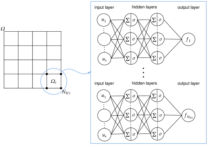
We will construct the surrogate mapping DtN~H,isubscript~DtN𝐻𝑖\widetilde{\text{DtN}}_{H,i} by learning the individual components of the original map. To learn this operator, we are using a fully-connected feed-forward neural network (NN). These networks are built as a sequence of layers including an input layer, hidden layers, and an output layer. Each layer performs an affine transformation followed by a nonlinear activation function σ:RR:𝜎maps-toRR\sigma:\mathrm{R}\mapsto\mathrm{R}. For each component DtN~H,ilsuperscriptsubscript~DtN𝐻𝑖𝑙\widetilde{\text{DtN}}_{H,i}^{l}, where l=1,,𝒩Ωi𝑙1subscript𝒩subscriptΩ𝑖l=1,\ldots,\mathscr{N}_{\partial{\Omega_{i}}}, we approximate it using a neural network expressed as a linear combination of functions:

DtN~H,il(θ;u)=φθkφθ1(u),superscriptsubscript~DtN𝐻𝑖𝑙𝜃𝑢superscriptsubscript𝜑𝜃𝑘superscriptsubscript𝜑𝜃1𝑢\widetilde{{\rm DtN}}_{H,i}^{l}(\theta;u)=\varphi_{\theta}^{k}\circ\ldots\circ\varphi_{\theta}^{1}(u),

where φθk(u)=σ(Wk(θ)u+𝐛k(θ))superscriptsubscript𝜑𝜃𝑘𝑢𝜎subscript𝑊𝑘𝜃𝑢subscript𝐛𝑘𝜃\varphi_{\theta}^{k}(u)=\sigma(W_{k}(\theta)u+\mathbf{b}_{k}(\theta)). The weights matrix Wksubscript𝑊𝑘W_{k} and biases 𝐛ksubscript𝐛𝑘\mathbf{b}_{k} are determined through training. We illustrate this concept with Figure 2.
Refer to caption
Figure 2. Representation of the learning workflow for the operator. Each neural network is depicted as a graph and will be responsible for learning each component of the DtN~H,isubscript~DtN𝐻𝑖\widetilde{\text{DtN}}_{H,i} operator. The first column of neurons (from left to right in NN) is the input layer, taking inputs (u1,u2,,us)subscript𝑢1subscript𝑢2subscript𝑢𝑠(u_{1},u_{2},\cdots,u_{s}) , and the last column is the output layer with output fNHiDtN~H,isubscript𝑓subscript𝑁𝐻𝑖subscript~DtN𝐻𝑖f_{N_{Hi}}\approx\widetilde{\text{DtN}}_{H,i}. The intermediate columns represent the hidden layers.

In NN methodology, the solution to the DtN operator is approximated by the following optimization process. Let U={us}s=1ns𝑈superscriptsubscriptsuperscript𝑢𝑠𝑠1subscript𝑛𝑠U=\{u^{s}\}_{s=1}^{n_{s}} be a set of sampling vectors sampled in the range (umin,umax)subscript𝑢minsubscript𝑢max(u_{\text{min}},u_{\text{max}}), where nssubscript𝑛𝑠n_{s} denotes the total number of sampling vectors. For each i=1,,N𝑖1𝑁i=1,\ldots,N and l=1,𝒩Ωi𝑙1subscript𝒩subscriptΩ𝑖l=1,\ldots\mathscr{N}_{\partial{\Omega_{i}}}, find θ=argmin𝜃(θ,U)superscript𝜃𝜃argmin𝜃𝑈\theta^{*}=\underset{\theta}{\mathrm{arg\,min}}\,\mathcal{L}(\theta,U), with

il(θ,U)superscriptsubscript𝑖𝑙𝜃𝑈\displaystyle\mathcal{L}_{i}^{l}(\theta,U) =c0i,0l(θ,U)+c1i,1l(θ,U)+cmoni,monl(θ)absentsubscript𝑐0superscriptsubscript𝑖0𝑙𝜃𝑈subscript𝑐1superscriptsubscript𝑖1𝑙𝜃𝑈subscript𝑐monsuperscriptsubscript𝑖mon𝑙𝜃\displaystyle=c_{0}\mathcal{L}_{i,0}^{l}(\theta,U)+c_{1}\mathcal{L}_{i,1}^{l}(\theta,U)+c_{\text{mon}}\mathcal{L}_{i,\text{mon}}^{l}(\theta) (30)

where c0subscript𝑐0c_{0}, c1subscript𝑐1c_{1} and cmonsubscript𝑐monc_{\text{mon}} are positive weights, i,0l(θ,u)superscriptsubscript𝑖0𝑙𝜃𝑢\mathcal{L}_{i,0}^{l}(\theta,u), i,1l(θ,u)superscriptsubscript𝑖1𝑙𝜃𝑢\mathcal{L}_{i,1}^{l}(\theta,u) and i,monl(θ)superscriptsubscript𝑖mon𝑙𝜃\mathcal{L}_{i,\text{mon}}^{l}(\theta) are defined by (31), (32) and (33) below.

For the loss function (30), we have error in sampled values given by

i,0l(θ,U)=1nss(DtN~H,il(θ;us)DtNH,il(us))2,superscriptsubscript𝑖0𝑙𝜃𝑈1subscript𝑛𝑠subscript𝑠superscriptsuperscriptsubscript~DtN𝐻𝑖𝑙𝜃superscript𝑢𝑠superscriptsubscriptDtN𝐻𝑖𝑙superscript𝑢𝑠2\mathcal{L}_{i,0}^{l}(\theta,U)=\dfrac{1}{n_{s}}\sum_{s}\left(\widetilde{\rm DtN}_{H,i}^{l}\left(\theta;u^{s}\right)-{\rm DtN}_{H,i}^{l}\left(u^{s}\right)\right)^{2}\,, (31)

and error with respective derivatives given by

i,1l(θ,U)=1nsk=1𝒩Ωis(ukDtN~H,il(θ;us)ukDtNH,il(us))2.superscriptsubscript𝑖1𝑙𝜃𝑈1subscript𝑛𝑠superscriptsubscript𝑘1subscript𝒩subscriptΩ𝑖subscript𝑠superscriptsubscriptsubscript𝑢𝑘superscriptsubscript~DtN𝐻𝑖𝑙𝜃superscript𝑢𝑠subscriptsubscript𝑢𝑘superscriptsubscriptDtN𝐻𝑖𝑙superscript𝑢𝑠2\mathcal{L}_{i,1}^{l}(\theta,U)=\dfrac{1}{n_{s}}\sum_{k=1}^{\mathscr{N}_{\partial{\Omega_{i}}}}\sum_{s}\left(\partial_{u_{k}}\widetilde{\rm DtN}_{H,i}^{l}\left(\theta;u^{s}\right)-\partial_{u_{k}}{\rm DtN}_{H,i}^{l}\left(u^{s}\right)\right)^{2}. (32)

In addition we introduce the monotonously loss terms defined either by

i,monl(θ)=(umin,umax)𝒩Ωi((ulDtN~H,il(θ;u)))2+kl((ukDtN~H,il(θ;u))+)2du,superscriptsubscript𝑖mon𝑙𝜃subscriptsuperscriptsubscript𝑢minsubscript𝑢maxsubscript𝒩subscriptΩ𝑖superscriptsuperscriptsubscriptsubscript𝑢𝑙superscriptsubscript~DtN𝐻𝑖𝑙𝜃𝑢2subscript𝑘𝑙superscriptsuperscriptsubscriptsubscript𝑢𝑘superscriptsubscript~DtN𝐻𝑖𝑙𝜃𝑢2𝑑𝑢\mathcal{L}_{i,\text{mon}}^{l}(\theta)=\int_{(u_{\text{min}},u_{\text{max}})^{\mathscr{N}_{\partial{\Omega_{i}}}}}\left(\left(\partial_{u_{l}}\widetilde{\rm DtN}_{H,i}^{l}\left(\theta;u\right)\right)^{-}\right)^{2}+\sum_{k\neq l}\left(\left(\partial_{u_{k}}\widetilde{\rm DtN}_{H,i}^{l}\left(\theta;u\right)\right)^{+}\right)^{2}du, (33)

or by

i,mon(θ)=(umin,umax)𝒩Ωi((ulDtN~H,il(θ;u)))2𝑑u,subscript𝑖mon𝜃subscriptsuperscriptsubscript𝑢minsubscript𝑢maxsubscript𝒩subscriptΩ𝑖superscriptsuperscriptsubscriptsubscript𝑢𝑙superscriptsubscript~DtN𝐻𝑖𝑙𝜃𝑢2differential-d𝑢\mathcal{L}_{i,\text{mon}}(\theta)=\int_{(u_{\text{min}},u_{\text{max}})^{\mathscr{N}_{\partial{\Omega_{i}}}}}\left(\left(\partial_{u_{l}}\widetilde{\rm DtN}_{H,i}^{l}\left(\theta;u\right)\right)^{-}\right)^{2}du, (34)

where (x)+=max(x,0)superscript𝑥𝑥0(x)^{+}=\max(x,0), (x)=min(x,0)superscript𝑥𝑥0(x)^{-}=\min(x,0) for any real x𝑥x, and where the integrals are taken over the training domain, which is an 𝒩Ωisubscript𝒩subscriptΩ𝑖\mathscr{N}_{\partial{\Omega_{i}}} dimensional cube. We note that i,monl(θ)superscriptsubscript𝑖mon𝑙𝜃\mathcal{L}_{i,\text{mon}}^{l}(\theta) does not require any data sampling. The purpose of this terms in the loss function is to enforce certain monotonicity properties that are expected from the original DtNH,isubscriptDtN𝐻𝑖{\rm DtN}_{H,i} maps. In particular, for one-dimensional problem, we expect the Jacobian of DtNH,isubscriptDtN𝐻𝑖{\rm DtN}_{H,i} to have positive diagonal elements and non-positive off-diagonal ones. We note that this property is closely related to the discrete maximum principle and is classical for Finite Volume methods. The loss term defined in (33) aims to penalize the wrong Jacobian signs. For problems in 2D, the off-diagonal elements of DtNH,isubscriptsuperscriptDtN𝐻𝑖{\rm DtN}^{\prime}_{H,i} do not have specific sign in general. Therefore, for such problems, we will be using (34) instead of (33). The monotonicity constrained based on (33) or (33) allows us to improve the robustness of Newton’s method for (29), which otherwise would be likely to fail.

For training, we generate DtNH,i(us)subscriptDtNHisuperscript𝑢𝑠{\rm DtN_{H,i}}(u^{s}) and DtNH,i(us)subscriptsuperscriptDtNHisuperscript𝑢𝑠{\rm DtN^{\prime}_{H,i}}(u^{s}) values for each sampling vector (us)s=1nssuperscriptsubscriptsuperscript𝑢𝑠𝑠1subscript𝑛𝑠(u^{s})_{s=1}^{n_{s}}. In terms of choosing sampling points to be used in training, we use a uniform sampling procedure.Given a sampling range (umin,umax)subscript𝑢𝑚𝑖𝑛subscript𝑢𝑚𝑎𝑥(u_{min},u_{max}), we sample each vector component with m𝑚m entries equally spaced between uminsubscript𝑢𝑚𝑖𝑛u_{min} and umaxsubscript𝑢𝑚𝑎𝑥u_{max}. Occasionally, these m𝑚m sampling points can also include additional points, particularly in the “center” of existing training points. This naturally leads to ns=m𝒩Ωisubscript𝑛𝑠superscript𝑚subscript𝒩subscriptΩ𝑖n_{s}=m^{\mathscr{N}_{\partial{\Omega_{i}}}} training vectors for the NN model, where (us)𝒩Ωisuperscript𝑢𝑠superscriptsubscript𝒩subscriptΩ𝑖(u^{s})\in\mathbb{R}^{\mathscr{N}_{\partial{\Omega_{i}}}}.

3. Numerical experiments

3.1. 1D degenerate elliptic problem

We first consider the following nonlinear equation

au(Kϵ(x)(u4))=0𝑎𝑢superscriptsubscript𝐾italic-ϵ𝑥superscriptsuperscript𝑢40au-\left(K_{\epsilon}(x)\left(u^{4}\right)^{\prime}\right)^{\prime}=0 (35)

posed in the domain (0,1)01(0,1) with some non-negative Dirichlet boundary conditions. The diffusion coefficient is given by

Kϵ(x)=102+12(1+sin(10πx+π4)),subscript𝐾italic-ϵ𝑥superscript10212110𝜋𝑥𝜋4K_{\epsilon}(x)=10^{-2}+\frac{1}{2}\left(1+\sin\left(10\pi x+\frac{\pi}{4}\right)\right),

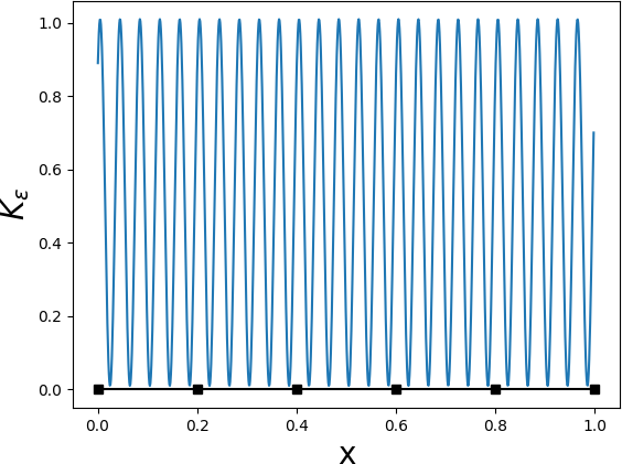
and a=20𝑎20a=20. Equation (35) can be interpreted as a stationary variant of the porous media equation [22]. It can be shown that u𝑢u takes values in [0,max(u(0),u(1)][0,\max(u(0),u(1)]. We note that, since the diffusion term in (35) degenerates at u=0𝑢0u=0, the solutions of (35) may vanish over some portion of the domain. The domain (0,1)01(0,1) is partitioned in five subdomains of equal size. We refer to Figure 3 for the illustration of the partitioning and the coefficient Kϵsubscript𝐾italic-ϵK_{\epsilon}.

Refer to caption
Figure 3. Partitioning of the model domain and the plot of Kϵ(x)subscript𝐾italic-ϵ𝑥K_{\epsilon}(x)

Because the partitioning of the domain is matching periodicity of Kϵ(x)subscript𝐾italic-ϵ𝑥K_{\epsilon}(x), the Dirichlet-to-Neumann operators coincide for all of the subdomains. As the analytical expression of the subdomain’s Dirichlet-to-Neumann operator is not available, the latter will be replaced by the approximate one denoted by DtNh,isubscriptDtN𝑖{\rm DtN}_{h,i} and computed by a finite element method using 200200200 grid points. To be more specific, we use 1subscript1\mathbb{P}_{1} finite element method with mass lumping. We note that in the one-dimensional case the mapping DtNh,isubscriptDtN𝑖{\rm DtN}_{h,i}, acting from 2superscript2\mathbb{R}^{2} to itself, coincides with the coarse operator DtNH,isubscriptDtN𝐻𝑖{\rm DtN}_{H,i} For surrogate model DtN~H,isubscript~DtN𝐻𝑖\widetilde{\rm DtN}_{H,i} we use fully connected neural network with two hidden layers of 64 neurons each. The activation function used in all the numerical experiment is given by σ(u)=max(u,0)2\sigma(u)=\max(u,0)^{2}. The model is trained over the domain [0,umax]2superscript0subscript𝑢𝑚𝑎𝑥2[0,u_{max}]^{2} with umax=4subscript𝑢𝑚𝑎𝑥4u_{max}=4. Training points are sampled over a regular grid in [0,umax]2superscript0subscript𝑢𝑚𝑎𝑥2[0,u_{max}]^{2} consisting of ns=22,32,42subscript𝑛𝑠superscript22superscript32superscript42n_{s}=2^{2},3^{2},4^{2} and 52superscript525^{2} points.

The loss function involves both values and derivatives of DtNH,isubscriptDtN𝐻𝑖{\rm DtN}_{H,i} at the sampling points with c0=1subscript𝑐01c_{0}=1 and c1=0.1subscript𝑐10.1c_{1}=0.1, as well as the monotonicity component (33) with cmon=4subscript𝑐𝑚𝑜𝑛4c_{mon}=4. The integral in (33) is approximated numerically based on integrand values over a regular 40×40404040\times 40 grid.

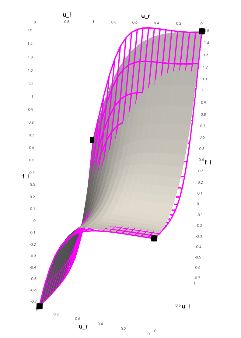
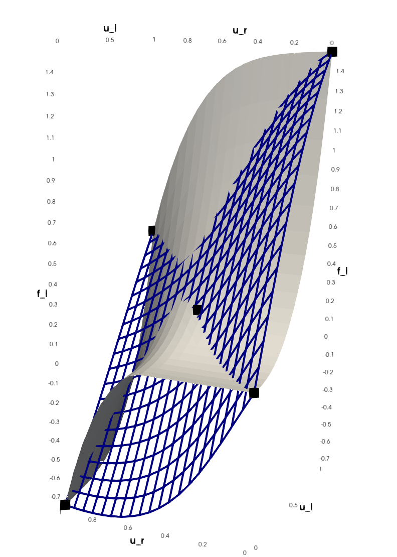
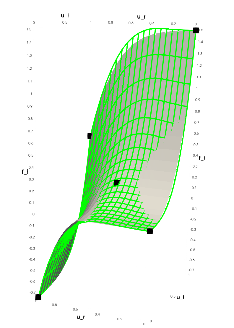
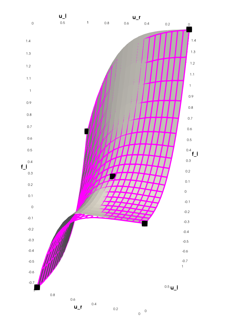
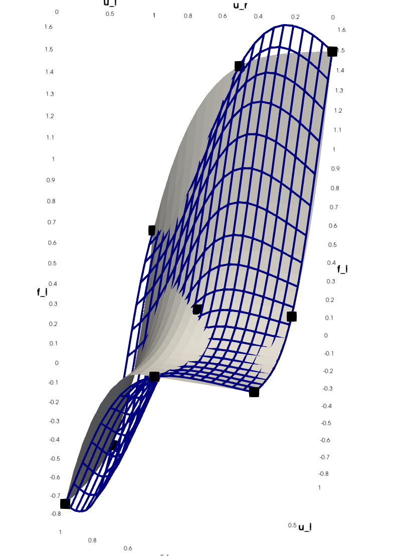
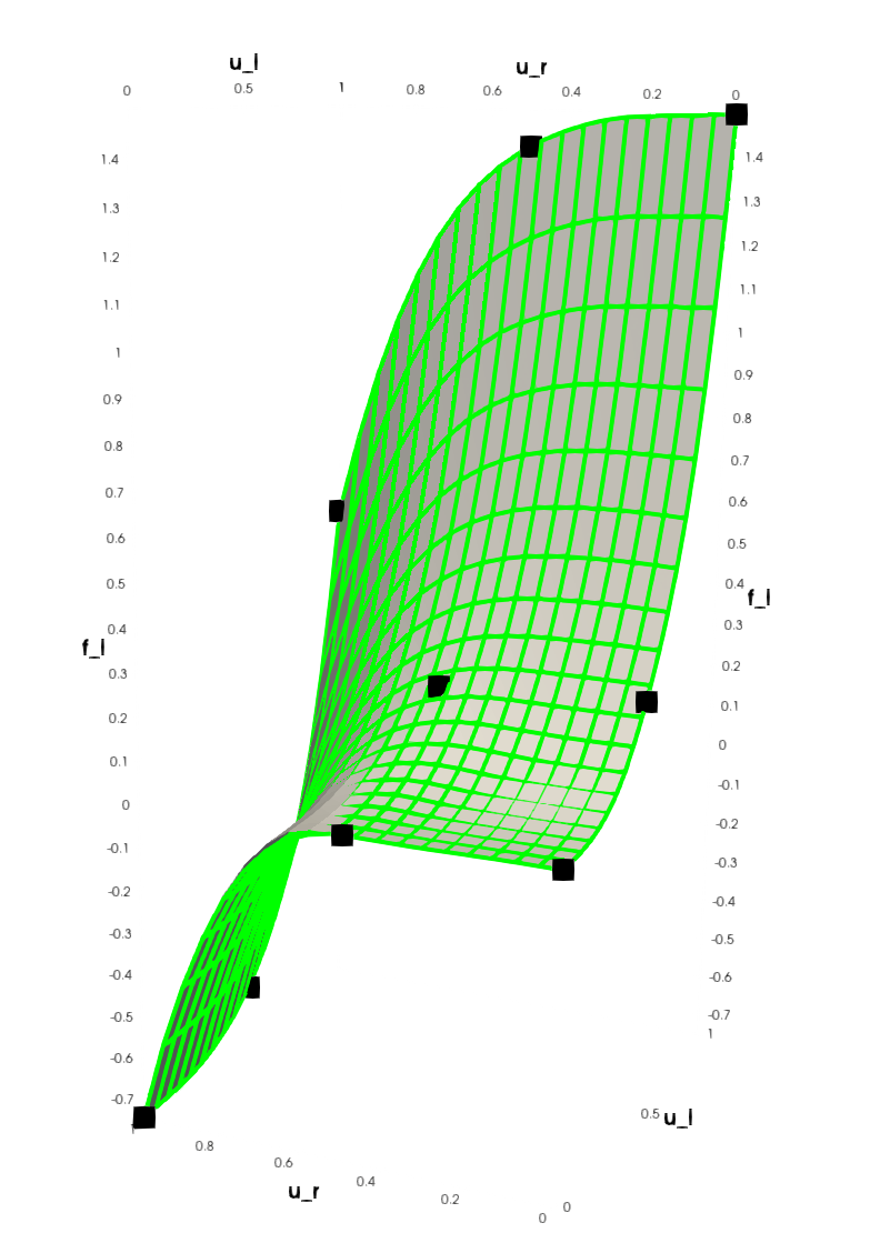
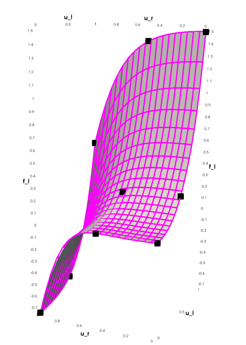
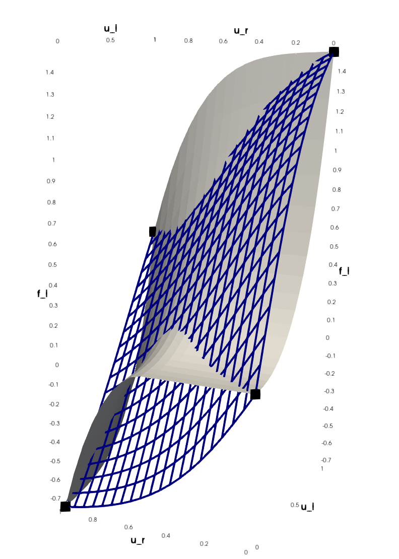
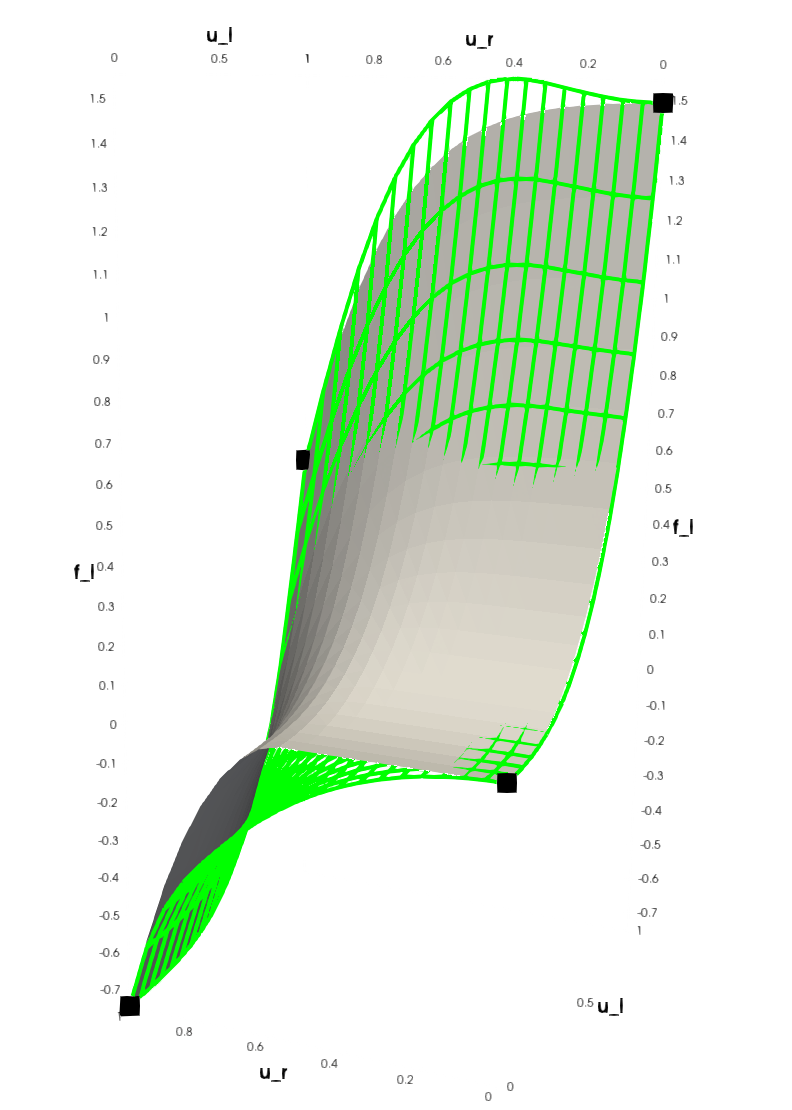
Let us begin with a qualitative analysis of the surrogate DtN~H,isubscript~DtN𝐻𝑖\widetilde{\rm DtN}_{H,i} model. Recall that, in 1D, DtNH,isubscriptDtN𝐻𝑖{\rm DtN}_{H,i} (coinciding with DtNh,isubscriptDtN𝑖{\rm DtN}_{h,i}) maps 2superscript2\mathbb{R}^{2} to itself, which can be interpreted as mapping left and right Dirichlet data to a pair of left and right fluxes. We report on Figure 4 the left flux and its surrogates as the function of the input Dirichlet values. The surface z=DtNH,i((uleft,uright))1𝑧subscriptDtN𝐻𝑖superscriptsubscript𝑢leftsubscript𝑢right1z={\rm DtN}_{H,i}((u_{\rm left},u_{\rm right}))^{1} shown as solid is the same for all sub-figures. Colored wireframe surfaces show z=DtN~H,i((uleft,uright))1𝑧subscript~DtN𝐻𝑖superscriptsubscript𝑢leftsubscript𝑢right1z=\widetilde{\rm DtN}_{H,i}((u_{\rm left},u_{\rm right}))^{1} for various number of sampling points (4, 5 and 9 for the first, second and third rows respectively), and different values of coefficients cαsubscript𝑐𝛼c_{\alpha} in (30) (same for each column). The results obtained using DtNDtN{\rm DtN} values alone (c1=0=cmon=0subscript𝑐10subscript𝑐𝑚𝑜𝑛0c_{1}=0=c_{mon}=0) are shown in the first column, those obtained using both values and derivatives (cmon=0subscript𝑐𝑚𝑜𝑛0c_{mon}=0) are reported in the middle column. Finally, the right column shows the outputs of the model using the additional monotonicity loss term (33). For the sake of clearer visualisation, here,the parameter a𝑎a is set to 1. Unsurprisingly, fitting not only the values, but also the tangential plains has a drastic benefit on the quality of the surrogate model (compare left and middle columns). Models with c1>0subscript𝑐10c_{1}>0 manage to capture the shape of the response surface reasonably well for very few training points. We also observe that adding the monotonicity loss does not seems to pollute the interpolation quality (middle versus right columns).

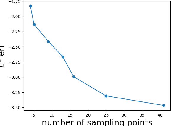
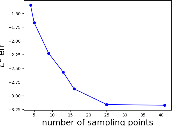
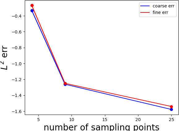
We report on Figure 5 convergence of the interpolation error of DtNH,isubscriptDtN𝐻𝑖{\rm DtN}_{H,i} in relative L2((0,umax)2)superscript𝐿2superscript0subscript𝑢𝑚𝑎𝑥2L^{2}((0,u_{max})^{2}) norm as the function of the number of sampling points. The error is evaluated over a regular 20×20202020\times 20 grid in [0,umax]2superscript0subscript𝑢𝑚𝑎𝑥2[0,u_{max}]^{2}. Here, in addition to the points sampled over regular ns×nssubscript𝑛𝑠subscript𝑛𝑠n_{s}\times n_{s} grid, we include additional points taken at the centers of the sampling grid cells. The decrease of error deteriorates after approximately 25 sampling points. This saturation effect (around error value of 103.5superscript103.510^{-3.5}) is even more clear in the second test case (see Figure 9 below). The failure in achieving higher accuracy should probably be attributed to our current training algorithm, combined with the fact that the structure of the surrogate model is fixed through the whole experiment.
Refer to caption
Refer to caption
Refer to caption
Refer to caption
Refer to caption
Refer to caption
Refer to caption
Refer to caption
Refer to caption
Figure 4. Qualitative comparison of the surfaces z=DtNH,i((uleft,uright))1𝑧subscriptDtN𝐻𝑖superscriptsubscript𝑢leftsubscript𝑢right1z={\rm DtN}_{H,i}((u_{\rm left},u_{\rm right}))^{1} (solid) and z=DtN~H,i((uleft,uright))1𝑧subscript~DtN𝐻𝑖superscriptsubscript𝑢leftsubscript𝑢right1z=\widetilde{\rm DtN}_{H,i}((u_{\rm left},u_{\rm right}))^{1} (wireframe). Left column (blue): only DtN values included. Middle column (green): DtN and DtN derivatives included. Right column (purple): DtN values, derivatives, and monotonicity assertion included. Top to bottom: ns=22subscript𝑛𝑠superscript22n_{s}=2^{2} training points, ns=22+1subscript𝑛𝑠superscript221n_{s}=2^{2}+1 training points, ns=32subscript𝑛𝑠superscript32n_{s}=3^{2} training points.
Refer to caption
Refer to caption
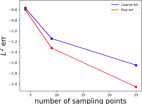
Figure 5. Left: Interpolation relative L2superscript𝐿2L^{2} error. Right: Solution relative L2superscript𝐿2L^{2} error.

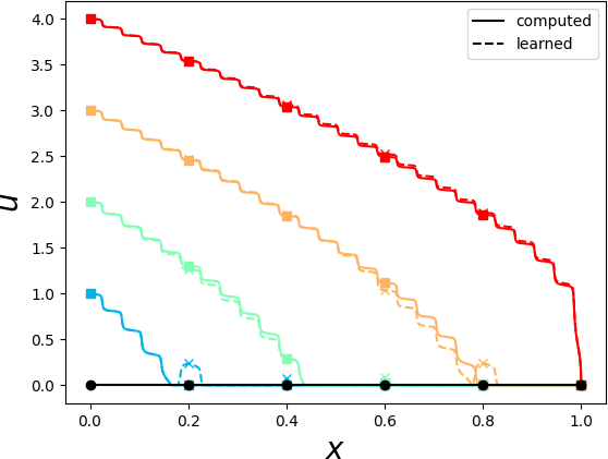
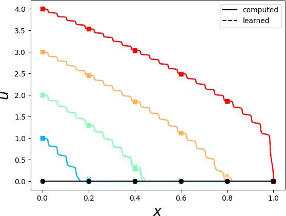
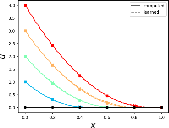
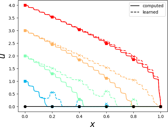
We further evaluate the performance of the surrogate models for the solution of the substructured problem (29), with u(1)=0𝑢10u(1)=0, and u(0)𝑢0u(0) taking values in {1,2,3,4}1234\{1,2,3,4\}. Once the coarse solution gHsubscript𝑔𝐻g_{H} and g~Hsubscript~𝑔𝐻\widetilde{g}_{H} are computed by approximately solving (28), and (29) respectively, we reconstruct the solution inside the subdomains by solving local problems on ΩisubscriptΩ𝑖{\Omega_{i}} with boundary condition given either by gH|Ωievaluated-atsubscript𝑔𝐻subscriptΩ𝑖g_{H}|_{\partial{\Omega_{i}}} or g~H|Ωievaluated-atsubscript~𝑔𝐻subscriptΩ𝑖\widetilde{g}_{H}|_{\partial{\Omega_{i}}}. Figure 6 reports the reconstructed solution, using both the original and the surrogate DtNDtN{\rm DtN} models, for different boundary conditions and varying number of sampling points. Starting from ns=32subscript𝑛𝑠superscript32n_{s}=3^{2} the surrogate model produced the solutions which are visually appear to be accurate. The relative L2(0,1)superscript𝐿201L^{2}(0,1) error as the function of the number of sampling points is reported by figure 5.
Refer to caption
Refer to caption
Refer to caption
Refer to caption
Figure 6. Solution profiles of (35) for various left boundary conditions using DtNH,isubscriptDtN𝐻𝑖{\rm DtN}_{H,i} (solid) and DtN~H,isubscript~DtN𝐻𝑖\widetilde{\rm DtN}_{H,i} (dashed) operators for ns=4,9,16subscript𝑛𝑠4916n_{s}=4,9,16 and 252525.

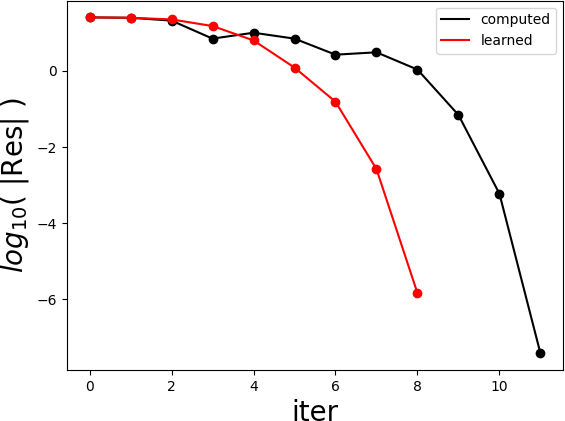
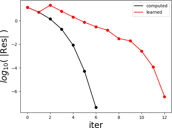
The numerical solution of (28) and (29) is obtained by Newton’s method. On Figure 7, we report typical convergence history for Newton’s method for the original (28) and the surrogate model (29) with u(0)=umax𝑢0subscript𝑢𝑚𝑎𝑥u(0)=u_{max} and ns=42subscript𝑛𝑠superscript42n_{s}=4^{2}. Here, the use of the surrogate model leads to convergence of Newton’s method with slightly fewer iterations. Most importantly, the inference time of DtN~~DtN\widetilde{\rm DtN} is much lower than the time required to evaluate DtNDtN{\rm DtN}.

Refer to caption
Figure 7. Convergence of Newton’s method using DtNH,isubscriptDtN𝐻𝑖{\rm DtN}_{H,i} (black) and DtN~H,isubscript~DtN𝐻𝑖\widetilde{\rm DtN}_{H,i} (red) operators to solve (35).

3.2. 1D plimit-from𝑝p-Laplace problem

Next, we consider the following equation

au(Kϵ(x)|u|2u)=0𝑎𝑢superscriptsubscript𝐾italic-ϵ𝑥superscriptsuperscript𝑢2superscript𝑢0au-\left(K_{\epsilon}(x)|u^{\prime}|^{2}u^{\prime}\right)^{\prime}=0 (36)

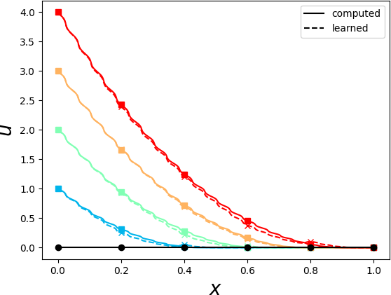
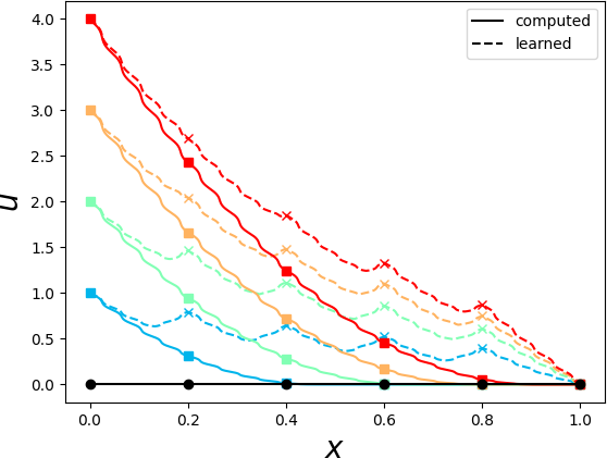
All the numerical parameters are set up as in the previous test case, except for the coefficient a=5𝑎5a=5. Again we compare the solution obtained using either the original or the surrogate substructured problem ((28) or (29)). Solution comparison for different boundary conditions and varying sampling point size is reported reported on Figure 8. Starting from ns=32subscript𝑛𝑠superscript32n_{s}=3^{2} the solution obtained using the surrogate model appears to be reasonably accurate. Figure 9 exhibits convergence of the relative interpolation and solution errors in L2((0,umax)2)superscript𝐿2superscript0subscript𝑢𝑚𝑎𝑥2L^{2}((0,u_{max})^{2}) and L2(0,1)superscript𝐿201L^{2}(0,1) norms,respectively. As before, we observe the saturation of the interpolation error as the function of nssubscript𝑛𝑠n_{s}; this phenomenon is even more pronounced than in the previous test case. Typical convergence of Newton’s method is shown by Figure 10 for u(0)=4𝑢04u(0)=4 and ns=42subscript𝑛𝑠superscript42n_{s}=4^{2}. Although Newton’s method requires twice as much iterations for the surrogate model compared to the original one, the former leads to a much faster algorithm due to a much lower inference time.
Refer to caption
Refer to caption
Refer to caption
Refer to caption
Figure 8. Solution profiles of (35) for various left boundary conditions using DtNH,isubscriptDtN𝐻𝑖{\rm DtN}_{H,i} (solid) and DtN~H,isubscript~DtN𝐻𝑖\widetilde{\rm DtN}_{H,i} (dashed) operators for ns=4,9,16subscript𝑛𝑠4916n_{s}=4,9,16 and 252525
Refer to caption
Refer to caption
Figure 9. Left: Interpolation relative L2superscript𝐿2L^{2} error. Right: Solution relative L2superscript𝐿2L^{2} error.
Refer to caption
Figure 10. Convergence of Newton’s method using DtNDtN{\rm DtN} (black) and DtN~~DtN\widetilde{\rm DtN} (red) operators to solve (36).

3.3. 2D degenerate elliptic problem

We consider a bi-dimensional version of (35) given by

udiv(Kϵ(x,y)u4)=0inΩ=(0,1)2,𝑢divsubscript𝐾italic-ϵ𝑥𝑦superscript𝑢40inΩsuperscript012missing-subexpressionmissing-subexpressionmissing-subexpression\begin{array}[]{rlllll}\displaystyle u-{\rm div}\left(K_{\epsilon}(x,y)\nabla u^{4}\right)=0&\mbox{in}&\Omega=(0,1)^{2},\\ \end{array} (37)

combined with the Dirichlet boundary conditions

u(x,y)=max(umax(x+y1),0)onΩ𝑢𝑥𝑦subscript𝑢𝑚𝑎𝑥𝑥𝑦10onΩu(x,y)=\max(u_{max}(x+y-1),0)\qquad\mbox{on}\qquad\partial\Omega

where umax=1.2subscript𝑢𝑚𝑎𝑥1.2u_{max}=1.2. That is, u(x,y)=0𝑢𝑥𝑦0u(x,y)=0 on lower and left boundaries and u(x,y)=umax(x+y1)𝑢𝑥𝑦subscript𝑢𝑚𝑎𝑥𝑥𝑦1u(x,y)=u_{max}(x+y-1) on right and top ones. We set

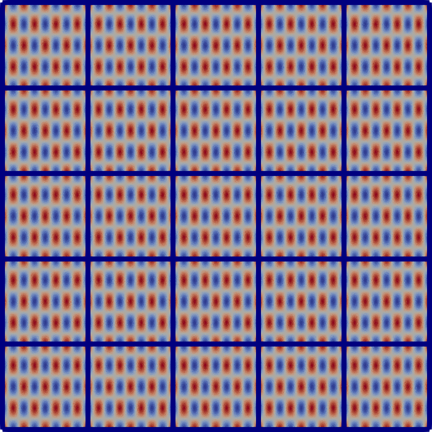
Kϵ(x,y)=102+12(1+sin(10x+π2)sin(5y+π2)),subscript𝐾italic-ϵ𝑥𝑦superscript10212110𝑥𝜋25𝑦𝜋2K_{\epsilon}(x,y)=10^{-2}+\frac{1}{2}\left(1+\sin\left(10x+\frac{\pi}{2}\right)\sin\left(5y+\frac{\pi}{2}\right)\right),

and we consider a regular partitioning of ΩΩ\Omega into 5×5555\times 5 subdomains (see Figure 11 for illustration). Here again, since the partitioning of the domain matches the periodicity of the coefficient Kϵsubscript𝐾italic-ϵK_{\epsilon}, one only needs to build a single surrogate DtNDtN{\rm DtN} model. More precisely, for every component of DtNH,ilsuperscriptsubscriptDtN𝐻𝑖𝑙{\rm DtN}_{H,i}^{l}, we train a specific model DtN~H,ilsuperscriptsubscript~DtN𝐻𝑖𝑙\widetilde{\rm DtN}_{H,i}^{l} using a fully connected neural network with 2 hidden layers of 202020 neurons each and the activation function σ(u)=max(u,0)2\sigma(u)=\max(u,0)^{2}.

Refer to caption
Refer to caption
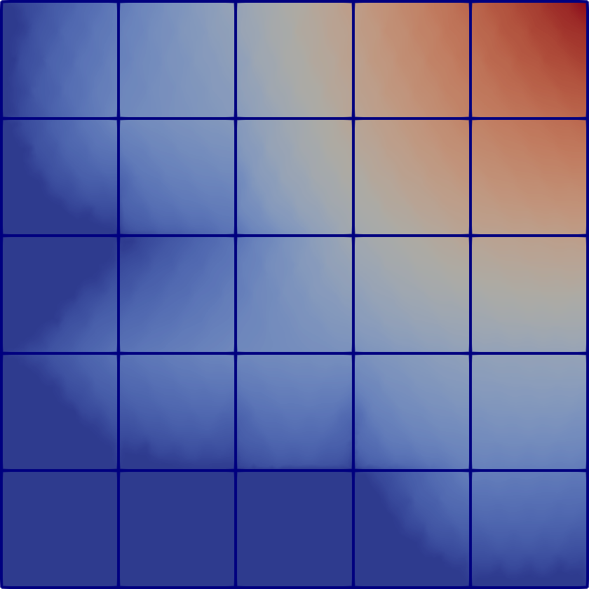
Figure 11. Left: Diffusion coefficient Kϵ(x)subscript𝐾italic-ϵ𝑥K_{\epsilon}(x). Right: Solution of model problem (37) using the original DtNH,isubscriptDtN𝐻𝑖{\rm DtN}_{H,i} operator.

The reference DtNH,isubscriptDtN𝐻𝑖{\rm DtN}_{H,i} operator is computed using mass lumped 1subscript1\mathbb{P}_{1} finite element method on a fine grid with approximately 660 triangles and 340 nodal degrees of freedom by subdomain. We report on Figure 11 the solution using this reference map. The training data is sampled on a regular grid over [0,umax]4superscript0subscript𝑢𝑚𝑎𝑥4[0,u_{max}]^{4}. The loss function uses both values and derivatives of DtNH,ilsuperscriptsubscriptDtN𝐻𝑖𝑙{\rm DtN}_{H,i}^{l} at the sampling points with c0=1subscript𝑐01c_{0}=1 and c1=0.1subscript𝑐10.1c_{1}=0.1. The monotonicity of DtN~H,ilsuperscriptsubscript~DtN𝐻𝑖𝑙\widetilde{\rm DtN}_{H,i}^{l} is enhanced by adding the loss term (34) with cmon=10subscript𝑐𝑚𝑜𝑛10c_{mon}=10. The integral in (34) is approximated by Monte Carlo method, using 200200200 random points sampled in [0,umax]4superscript0subscript𝑢𝑚𝑎𝑥4[0,u_{max}]^{4} at every optimisation step.

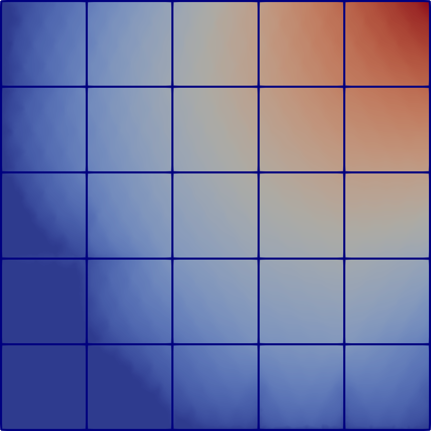
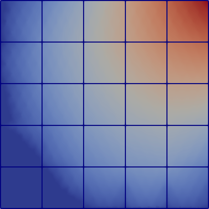
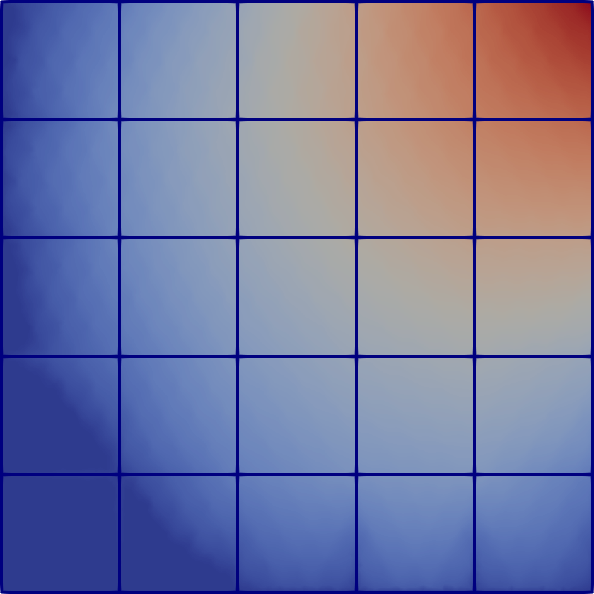
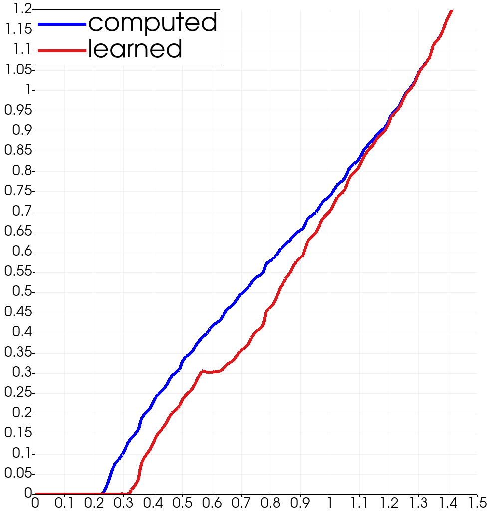
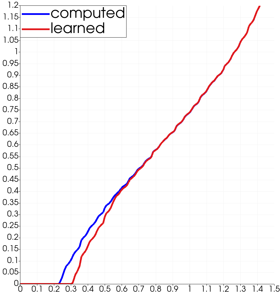
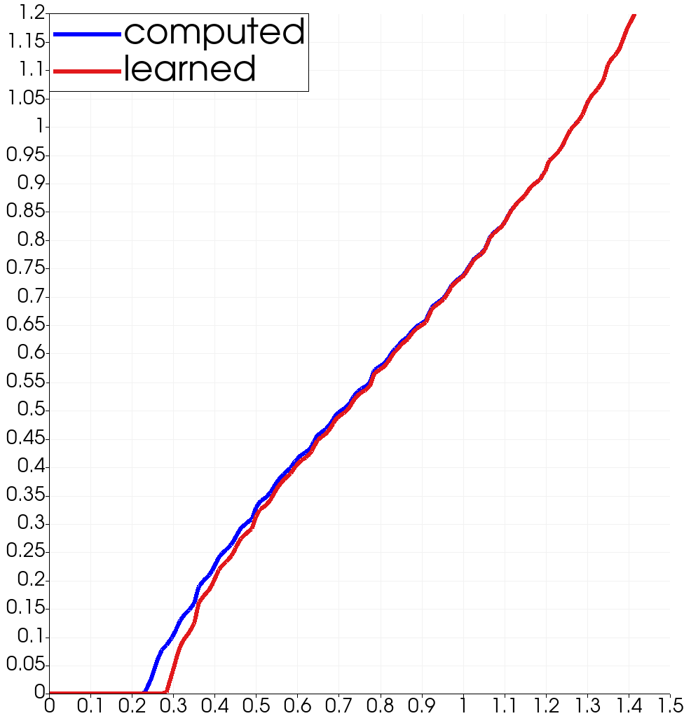
The solution obtained using the surrogate models trained with ns=24,34,44subscript𝑛𝑠superscript24superscript34superscript44n_{s}=2^{4},3^{4},4^{4} and 54superscript545^{4} are reported on Figure 12, together with solution profiles along the line x=y𝑥𝑦x=y shown on Figure 13.

nssubscript𝑛𝑠n_{s} 24superscript242^{4} 34superscript343^{4} 44superscript444^{4} 54superscript545^{4}
Rel. error 33%percent3333\% 8%percent88\% 4%percent44\% 3%percent33\%
Table 1. Relative L2(Ω)superscript𝐿2ΩL^{2}(\Omega) error between surrogate model and true models.

We observe that the error decreases as the number of sampling points grows, with the relative L2(Ω)superscript𝐿2ΩL^{2}(\Omega) being below 10%percent1010\% starting from ns=34subscript𝑛𝑠superscript34n_{s}=3^{4}.

Refer to caption
Refer to caption
Refer to caption
Refer to caption
Figure 12. Solution of model problem (37) using learned DtN~~DtN\widetilde{\rm DtN} map for various numbers of sampling points, including ns=24subscript𝑛𝑠superscript24n_{s}=2^{4} (top left), ns=34subscript𝑛𝑠superscript34n_{s}=3^{4} (top right), ns=44subscript𝑛𝑠superscript44n_{s}=4^{4} (bottom left), and ns=54subscript𝑛𝑠superscript54n_{s}=5^{4} (bottom right).
Refer to caption
Refer to caption
Refer to caption
Refer to caption
Figure 13. Original (blue) and surrogate (red) reconstructed solution along the line y=x𝑦𝑥y=x for ns=24subscript𝑛𝑠superscript24n_{s}=2^{4} (top left), ns=34subscript𝑛𝑠superscript34n_{s}=3^{4} (top right), ns=44subscript𝑛𝑠superscript44n_{s}=4^{4} (bottom left) and ns=54subscript𝑛𝑠superscript54n_{s}=5^{4} (bottom right)

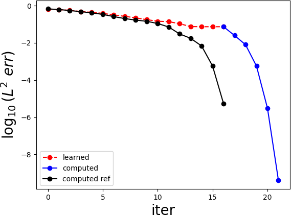
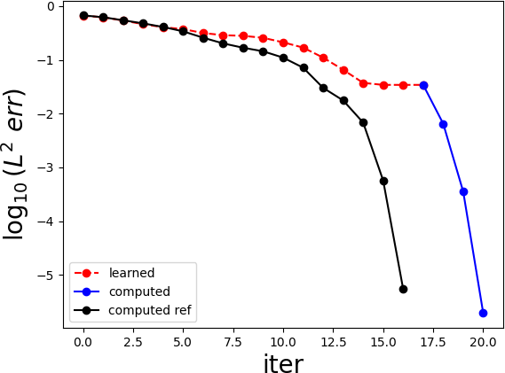
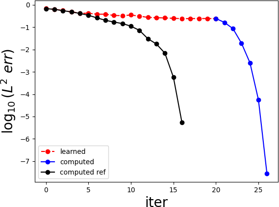
Let us recall that the evaluation of the residual function (27) based on the original coarse DtNH,isubscriptDtN𝐻𝑖{\rm DtN}_{H,i} operator requires the solution of the family of local nonlinear finite element systems, which is computationally demanding. In contrast, the inference time of DtN~H,isubscript~DtN𝐻𝑖\widetilde{\rm DtN}_{H,i} is very low, allowing for fast computation of the solution to the surrogate system (29). (X). Although the surrogate solution g~Hsubscript~𝑔𝐻\widetilde{g}_{H} may not be sufficiently accurate, it can serve to initialize the nonlinear solver for the original coarse problem (28). This idea is illustrated by Figure 14. Figure 14 reports convergence of the relative L2(Ω)superscript𝐿2ΩL^{2}(\Omega) error between a very accurate solution to (28) and the current Newton’s method iterate obtained using either using DtN~H,isubscript~DtN𝐻𝑖\widetilde{\rm DtN}_{H,i} or DtNH,isubscriptDtN𝐻𝑖{\rm DtN}_{H,i} with different initialization. The black curve shows convergence of Newton’s method for the original problem (28) starting from zero initial guess and is the same for all three sub-figures. Similarly, the red curves depict convergence of Newton’s method for the surrogate problem (29) for various number ns=24,34subscript𝑛𝑠superscript24superscript34n_{s}=2^{4},3^{4} and 44superscript444^{4}, again starting for zero initial guess. The stagnation of the red curve is results the approximation error associated to DtN~H,isubscript~DtN𝐻𝑖\widetilde{\rm DtN}_{H,i}. Finally, the blue curve shows convergence of Newton’s method for (28) starting from the surrogate solution. For the original coarse problem, convergence up to the tolerance of 105superscript10510^{-5} is obtained within 17 iterations. In contrast, the Newton’s method initialized by the surrogate solution requires up to 4 times fewer iterations in order to achieve the similar accuracy. In particular, there are only 7, 5 or 4 iterations needed for ns=24,34subscript𝑛𝑠superscript24superscript34n_{s}=2^{4},3^{4} and 44superscript444^{4}, respectively. Note that even when using a very crude ns=2subscript𝑛𝑠2n_{s}=2 surrogate model, a significant reduction of Newton’s step is achieved.
Refer to caption
Refer to caption
Refer to caption
Figure 14. L2superscript𝐿2L^{2} error between the reference solution and the current iterate of Newton’s method for (29) using zero initial guess (red), and (28) with either initial guess set to zero (black) or provided by the approximate solution of (29). Top row from left to right, ns=24,34subscript𝑛𝑠superscript24superscript34n_{s}=2^{4},3^{4}, bottom row ns=44subscript𝑛𝑠superscript44n_{s}=4^{4}

4. Conclusion and outlook

We have presented the framework that combines the Multi-scale Finite Element (MsFEM) method with techniques from Machine Learning, providing an extension of the former to the case of nonlinear PDEs with highly oscilatory coefficients. Our approach relies on learning Dirichlet-to-Neumann (DtN) maps acting between some low-dimensional (coarse) spaces. The surrogate DtN operators are further combined together within a global substructured formulation solved by Newton’s method. The optimization process involves fitting values and derivatives of the true coarse DtN, where incorporating derivative information into the loss function plays a pivotal role in accuracy of the learned operator. In addition, we weakly enforce some monotonicity properties of the original model, which improves the performance of Newton’s method.

Numerical experiments, performed in 1D and 2D and involving challenging plimit-from𝑝p-Laplace and degenerate diffusion equations, have shown promising results. With just a few training points by dimension, the substitution model can approach the solution with an accuracy of a few percent. A further improvement in the accuracy can be achieved by using the “learned” solution as an initial guess for Newton’s method applied to the original (not learned) substructured formulation, allowing us to enter directly into the region of quadratic convergence and obtain a more accurate “learned” solution. Although the our numerical experiment has been so far limited to the case of periodically distributed coefficients, the extension to the non-periodic case is trivial and will be carried out in the future. Future work also involves incorporating techniques from Principal Component Analysis (PCA) to reduce complexity associated to the derivatives of the DtN. Additionally, the inclusion of higher-order derivatives could increase model accuracy. Higher-order optimizers like BFGS, which incorporates curvature/Hessian information into the loss function, may improve the convergence of the loss function.

References

  • [1] Babuska, I., Caloz, G., Osborn, J.E.: Special finite element methods for a class of second order elliptic problems with rough coefficients. SIAM Journal on Numerical Analysis 31(4), 945–981 (1994)
  • [2] Babuska, I., Lipton, R.: Optimal local approximation spaces for generalized finite element methods with application to multiscale problems. Multiscale Modeling and Simulation 9(1), 373–406 (2011)
  • [3] Badia, S., Li, W., Martín, A.F.: Finite element interpolated neural networks for solving forward and inverse problems. arXiv preprint arXiv:2306.06304 (2023)
  • [4] Cai, S., Wang, Z., Wang, S., Perdikaris, P., Karniadakis, G.E.: Physics-informed neural networks for heat transfer problems. Journal of Heat Transfer 143(6) (2021)
  • [5] Chaturantabut, S., Sorensen, D.C.: Nonlinear model reduction via discrete empirical interpolation. SIAM Journal on Scientific Computing 32(5), 2737–2764 (2010)
  • [6] Dolean, V., Jolivet, P., Nataf, F.: An introduction to domain decomposition methods: algorithms, theory, and parallel implementation. SIAM (2015)
  • [7] Efendiev, Y., Galvis, J., Hou, T.Y.: Generalized multiscale finite element methods (gmsfem). Journal of computational physics 251, 116–135 (2013)
  • [8] Hou, T.Y., Wu, X.H.: A multiscale finite element method for elliptic problems in composite materials and porous media. Journal of computational physics 134(1), 169–189 (1997)
  • [9] Huge, B., Savine, A.: Differential machine learning. arXiv preprint arXiv:2005.02347 (2020)
  • [10] Jagtap, A.D., Karniadakis, G.E.: Extended physics-informed neural networks (xpinns): A generalized space-time domain decomposition based deep learning framework for nonlinear partial differential equations. In: AAAI Spring Symposium: MLPS (2021)
  • [11] Jagtap, A.D., Kharazmi, E., Karniadakis, G.E.: Conservative physics-informed neural networks on discrete domains for conservation laws: Applications to forward and inverse problems. Computer Methods in Applied Mechanics and Engineering 365, 113028 (2020)
  • [12] Kharazmi, E., Zhang, Z., Karniadakis, G.E.: Variational physics-informed neural networks for solving partial differential equations. arXiv preprint arXiv:1912.00873 (2019)
  • [13] Leray, J., Lions, J.: Quelques résultats de visik sur les problèmes elliptiques non linéaires par les méthodes de minty-browder. Séminaire Jean Leray (1), 1–19 (1964)
  • [14] Lu, L., Jin, P., Pang, G., Zhang, Z., Karniadakis, G.E.: Learning nonlinear operators via deeponet based on the universal approximation theorem of operators. Nature machine intelligence 3(3), 218–229 (2021)
  • [15] Ma, C., Scheichl, R., Dodwell, T.: Novel design and analysis of generalized finite element methods based on locally optimal spectral approximations. SIAM Journal on Numerical Analysis 60(1), 244–273 (2022)
  • [16] Målqvist, A., Peterseim, D.: Localization of elliptic multiscale problems. Mathematics of Computation 83(290), 2583–2603 (2014)
  • [17] Mao, Z., Jagtap, A.D., Karniadakis, G.E.: Physics-informed neural networks for high-speed flows. Computer Methods in Applied Mechanics and Engineering 360, 112789 (2020)
  • [18] Misyris, G.S., Venzke, A., Chatzivasileiadis, S.: Physics-informed neural networks for power systems. In: 2020 IEEE Power & Energy Society General Meeting (PESGM), pp. 1–5. IEEE (2020)
  • [19] Moseley, B., Markham, A., Nissen-Meyer, T.: Finite basis physics-informed neural networks (fbpinns): a scalable domain decomposition approach for solving differential equations. Advances in Computational Mathematics 49(4), 62 (2023)
  • [20] Ortega, J.M., Rheinboldt, W.C.: Iterative solution of nonlinear equations in several variables. SIAM (2000)
  • [21] Raissi, M., Perdikaris, P., Karniadakis, G.E.: Physics-informed neural networks: A deep learning framework for solving forward and inverse problems involving nonlinear partial differential equations. Journal of Computational physics 378, 686–707 (2019)
  • [22] Vázquez, J.L.: The porous medium equation: mathematical theory. Oxford University Press (2007)
  • [23] Weinan, E., Engquist, B.: The heterogeneous multiscale methods. Communications in Mathematical Sciences 1(1), 87–132 (2003)