Optimizing Information Freshness in IoT Systems with Update Rate Constraints: A Token-Based Approach

Erfan Delfani1, and Nikolaos Pappas1
Email: {erfan.delfani, nikolaos.pappas}@liu.se
This work has been supported in part by the Swedish Research Council (VR), ELLIIT, and the European Union (ETHER, 101096526, ELIXIRION, 101120135, and SOVEREIGN, 101131481).ISBN 978-3-903176-63-8 ©©\copyright 2024 IFIP 1Department of Computer and Information Science, Linköping University, Linköping, Sweden
Abstract

In Internet of Things (IoT) status update systems, where information is sampled and subsequently transmitted from a source to a destination node, the imperative necessity lies in maintaining the timeliness of information and updating the system with optimal frequency. Optimizing information freshness in resource-limited status update systems often involves Constrained Markov Decision Process (CMDP) problems with update rate constraints. Solving CMDP problems, especially with multiple constraints, is a challenging task. To address this, we present a token-based approach that transforms CMDP into an unconstrained MDP, simplifying the solution process. We apply this approach to systems with one and two update rate constraints for optimizing Age of Incorrect Information (AoII) and Age of Information (AoI) metrics, respectively, and explore the analytical and numerical aspects. Additionally, we introduce an iterative triangle bisection method for solving the CMDP problems with two constraints, comparing its results with the token-based MDP approach. Our findings show that the token-based approach yields superior performance over baseline policies, converging to the optimal policy as the maximum number of tokens increases.

I Introduction

Prudent control of status updates to provide timely information exchange in resource-limited IoT networks has emerged as an important research direction within semantics-aware goal-oriented communication. In these systems, update packets from an information source are generated and transmitted through a communication network to a destination node for subsequent processing and utilization. This process fulfills application-driven goals, including remote actuator control in industrial automation, steering autonomous vehicles in intelligent transportation systems, and monitoring health and environmental status[1, 2, 3]. In such time-sensitive systems, the reliability and accuracy of controls depend on the timeliness of information. Therefore, there is a high demand for the freshness of information and, consecutively, for frequent generation of updates. However, due to resource limitations arising from factors such as energy limitations, channel accessibility, or processing capacity, it is crucial to optimize the timing and the amount of generated, transmitted, or processed data within a network. This results in problems addressing the optimization of information freshness under updating rate constraints, aiming to find optimal policies that answer the question of when to generate or transmit update packets. In the literature of status update systems, the quantification of information freshness is accomplished through timing metrics, such as Age of Information (AoI) [1], Age of Incorrect Information (AoII) [4], Version AoI (VAoI) [5], and Age of Actuation (AoA) [6], each metric addressing distinct aspects of timing and importance of information.

Below, we present and discuss papers that consider the optimization of information freshness in status update systems under rate constraints. [7] minimizes average AoI by scheduling updates over an error-prone channel with transmission constraints, studying optimal policies under various feedback mechanisms. [8] addresses minimizing average AoI under transmission power constraints, transforming the problem into an unconstrained MDP through Lagrangian relaxation. [4] introduces AoII metric and solves the CMDP problem with a Lagrangian approach. [9] focuses on fresh data collection from power-constrained sensors in IIoT networks, optimizing average AoI with scheduling algorithms and LP-based optimization. [10] minimizes AoI in wireless networks with peak power-constrained base stations, using CMDP with strict and relaxed power constraints and proposing a truncated multi-user scheduling policy. [11] minimizes average AoI in resource-constrained IoT networks using a CMDP model and Lagrangian multipliers, offering an asymptotically optimal, low-complexity algorithm. The works mentioned above primarily rely on formulating the constrained optimization problem using the CMDP framework and subsequently proceed to solve it through a Lagrangian approach.

However, solving a CMDP problem through the direct primary formulation or the Lagrangian dual approach presents a formidable challenge, particularly for problems with multiple constraints[12]. To address this challenge, we present a token-based approach for transforming the CMDP problem into an unconstrained MDP problem, following the same approach in [13]. The resulting MDP can be directly solved using popular iterative standard methods. Specifically, we convert the constrained problem into an unconstrained problem by defining new variables within the system model. These variables are defined in such a way as to ensure the update rate constraints. To elaborate, drawing inspiration from the well-known token bucket mechanism, a commonly referenced concept in the literature [14, 15, 16, 13], we allocate a specific number of tokens to the system in each time slot (or assign one token with a specific probability) for potential updates. When the tokens accumulate sufficiently, the system can decide whether to spend them and update or refrain from updating. This way, the system can optimize update actions by spending tokens at the right time by solving an unconstrained MDP. For single rate constraint problems, this approach resembles the idea of modifying the system model and incorporating an Energy Harvesting (EH) sensor with a random energy arrival for sampling and status updating [17, 18, 19, 20, 21, 22, 23]. However, as we will demonstrate in subsequent sections by applying it to two rate constrained problems, this token-based approach can be effectively applied to general system models, without being limited to EH scenarios. Our contributions are as follows:

  • We present a token-based unconstrained MDP for optimizing AoII in a status update system derived from a single-rate constrained MDP and provide analytical results.

  • We formulate a two-rate constrained MDP and its corresponding token-based unconstrained MDP for optimizing AoI in a status update system. Analytical results for the unconstrained problem are presented.

  • We introduce an iterative triangle bisection method for solving the CMDP with two constraints.

  • Finally, we compare the performance of the optimal token-based policy in different setups with that of the optimal policy for the primary CMDP and other baseline policies through numerical analysis.

II System Model

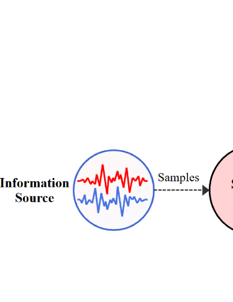
We consider a status update system depicted in Fig. 1, where update packets/samples originating from an information source are generated and transmitted from a source node (Tx) to a destination node (Rx) within a network, by an update policy. This policy dictates when the update packets are transmitted to the destination nodes, and our objective is to ascertain the optimal policy that maximizes performance by optimizing information freshness within the system while adhering to maximum allowable update rates. In this system model, the update packets are forwarded through a channel, which may be reliable or unreliable. Additionally, we integrate a channel from the receiver to the transmitter, which can be utilized to either transmit acknowledgment feedback (in a push-based scenario) or request a new update (in a pull-based scenario), as in [24] and [25]. We presume the backward channel to be error-free and instantaneous. The proposed token-based approach is versatile and can be applied to optimize various information freshness metrics across diverse system configurations. In what follows, we investigate the CMDP and token-based problems to optimize AoII and AoI in two distinct system setups under one and two update rate constraints, respectively, in Sections III and IV. AoI is a performance metric that quantifies the freshness of information, defined as the time elapsed since the generation time of the last successfully received update at the destination node. AoII quantifies the time elapsed since the latest instance when the source collected a sample with identical content to the current sample stored at the destination. In this system model, we assume that the time is slotted and the slots are of equal duration.
Refer to caption
Figure 1: A general system model for optimizing information freshness under update rate constraints.

III A system with single rate constraint

III-A Problem Formulation

In a status update system, as depicted in Fig. 1, where the objective is to optimize the time average of a freshness metric or a cost function C(s(t),a(t))𝐶𝑠𝑡𝑎𝑡C\big{(}s\left(t\right),a\left(t\right)\big{)} subject to an update rate constraint, a CMDP problem can be defined as follows:

minπΠsubscript𝜋Π\displaystyle\min_{\pi\in\Pi}\ lim supT1TE[t=0T1C(sπ(t),aπ(t))|s(0)],subscriptlimit-supremum𝑇1𝑇𝐸delimited-[]conditionalsuperscriptsubscript𝑡0𝑇1𝐶superscript𝑠𝜋𝑡superscript𝑎𝜋𝑡𝑠0\displaystyle\limsup_{T\rightarrow\infty}{\frac{1}{T}E\left[\sum_{t=0}^{T-1}C\big{(}s^{\pi}(t),a^{\pi}(t)\big{)}\Big{|}s(0)\right]}, (1)
s.t. lim supT1TE[t=0T1aπ(t)|s(0)]α,subscriptlimit-supremum𝑇1𝑇𝐸delimited-[]conditionalsuperscriptsubscript𝑡0𝑇1superscript𝑎𝜋𝑡𝑠0𝛼\displaystyle\limsup_{T\rightarrow\infty}{\frac{1}{T}E\left[\sum_{t=0}^{T-1}a^{\pi}(t)\Big{|}s(0)\right]}\leq\alpha,

where the policy π𝜋\pi is a sequence of actions, i.e., π=def(aπ(0),aπ(1),aπ(2),)𝜋defsuperscript𝑎𝜋0superscript𝑎𝜋1superscript𝑎𝜋2\pi\overset{\text{def}}{=}\big{(}a^{\pi}(0),a^{\pi}(1),a^{\pi}(2),\cdots\big{)}, where aπ(t){0,1}superscript𝑎𝜋𝑡01a^{\pi}(t)\in\{0,1\} represents the action at time t𝑡t. Here, aπ(t)=1superscript𝑎𝜋𝑡1a^{\pi}(t)=1 represents the update action, whereas aπ(t)=0superscript𝑎𝜋𝑡0a^{\pi}(t)=0 indicates the no-update action. The term update refers to the process of generating and transmitting information from the source to the destination. sπ(t)superscript𝑠𝜋𝑡s^{\pi}(t) is the state of the system under the policy π𝜋\pi, including a timeliness or freshness variable. In this formulation, the parameter 0<α<10𝛼10<\alpha<1 restricts the average update rate. We omit the superscript π𝜋\pi in our analysis to facilitate presentation.

To transform this CMDP problem into the token-based MDP one, we define a new state vector s^(t)=def[b(t),s(t)]^𝑠𝑡def𝑏𝑡𝑠𝑡\hat{s}(t)\overset{\text{def}}{=}[b(t),s(t)], where b(t){0,1,2,,bmax}𝑏𝑡012subscript𝑏𝑚𝑎𝑥b(t)\in\{0,1,2,\ldots,b_{max}\} is a token variable evolving as:

b(t+1)={b(t)a(t)+1with probability α,b(t)a(t)with probability 1α,𝑏𝑡1cases𝑏𝑡𝑎𝑡1with probability 𝛼𝑏𝑡𝑎𝑡with probability 1𝛼\displaystyle b(t+1)=\begin{cases}b(t)-a(t)+1&\text{with probability }\alpha,\\ b(t)-a(t)&\text{with probability }1-\alpha,\\ \end{cases} (2)

where we have assumed that each update consumes one token. The action a(t)𝑎𝑡a(t) must be set to zero (indicating no update) when b(t)𝑏𝑡b(t) is equal to zero. Otherwise, when b(t)>0𝑏𝑡0b(t)>0, the system will decide on the optimal action at each time slot. This optimal policy can be obtained by solving the following token-based unconstrained MDP problem:

minπΠlim supT1TE[t=0T1C(s^π(t),aπ(t))|s^(0)],subscript𝜋Πsubscriptlimit-supremum𝑇1𝑇𝐸delimited-[]conditionalsuperscriptsubscript𝑡0𝑇1𝐶superscript^𝑠𝜋𝑡superscript𝑎𝜋𝑡^𝑠0\displaystyle\min_{\pi\in\Pi}\ \limsup_{T\rightarrow\infty}{\frac{1}{T}E\Bigg{[}\sum_{t=0}^{T-1}C\Big{(}\hat{s}^{\pi}(t),a^{\pi}(t)\Big{)}\Big{|}\hat{s}(0)\Bigg{]}}, (3)

where the cost function is the same as the CMDP problem (1), and the transition probabilities of this new MDP problem can be simply derived using the transition probability of the main CMDP problem, via the following equation:

P[s^(t+1)|s^(t),a(t)]=P[b(t+1),s(t+1)|b(t),s(t),a(t)]=P[b(t+1)|b(t),a(t)]Can be derived from (2)×P[s(t+1)|s(t),a(t)]Given by CMDP problem (1).𝑃delimited-[]conditional^𝑠𝑡1^𝑠𝑡𝑎𝑡𝑃𝑏𝑡1conditional𝑠𝑡1𝑏𝑡𝑠𝑡𝑎𝑡subscript𝑃delimited-[]conditional𝑏𝑡1𝑏𝑡𝑎𝑡Can be derived from (2)subscript𝑃delimited-[]conditional𝑠𝑡1𝑠𝑡𝑎𝑡Given by CMDP problem (1)P\big{[}\hat{s}(t\!+\!1)\big{|}\hat{s}(t),a(t)\big{]}\!=\!P\big{[}b(t\!+\!1),s(t\!+\!1)\big{|}b(t),s(t),a(t)\big{]}\\ =\underbrace{P\big{[}b(t+1)\big{|}b(t),a(t)\big{]}}_{\text{Can be derived from \eqref{bEvol_eqn}}}\times\underbrace{P\big{[}s(t+1)\big{|}s(t),a(t)\big{]}}_{\text{Given by CMDP problem \eqref{CMDP_eqn}}}. (4)

III-B Optimizing AoII under rate constraint

In a scenario where the cost function is defined to be AoII, denoted by ΔAoII(t)superscriptΔAoII𝑡\Delta^{\text{AoII}}(t), the CMDP problem (1) has previously been addressed for a specific system model [4]. The considered system model focuses on a communication system involving a transmitter-receiver pair where the transmitter sends status updates about a discrete Markov chain process to the receiver over an unreliable channel, as depicted in Fig. 1. The process has N𝑁N states, and probabilities of staying in the same state (pRsubscript𝑝𝑅p_{R}) or transitioning to another state (ptsubscript𝑝𝑡p_{t}) are defined such that pR+(N1)pt=1subscript𝑝𝑅𝑁1subscript𝑝𝑡1p_{R}+(N-1)p_{t}=1. The unreliable channel follows a Bernoulli distribution with success (pssubscript𝑝𝑠p_{s}) and failure (pf=1pssubscript𝑝𝑓1subscript𝑝𝑠p_{f}=1-p_{s}) probabilities at each time slot. Successful transmission prompts an ACK feedback, while failure results in a NACK. The transmitter can perfectly estimate the receiver’s information source using these packets. The transmitter follows a push-based scenario and generates updates at its discretion by sampling the current process state. The objective is to minimize the time-average AoII with the adopted transmission policy.

This problem can be formulated as a CMDP presented in (1), where the state at time t𝑡t is characterized by the AoII, s(t)=defΔAoII(t){0,1,2,,Δmax}𝑠𝑡defsuperscriptΔAoII𝑡012subscriptΔmaxs(t)\overset{\text{def}}{=}\Delta^{\text{AoII}}(t)\in\{0,1,2,\cdots,\Delta_{\text{max}}\}. The action at time t𝑡t, denoted as a(t){0,1}𝑎𝑡01a(t)\in\{0,1\}, signifies an attempted update (value 111) or remaining idle (value 00). The instantaneous cost is defined as C(s(t),a(t))=defΔAoII(t)𝐶𝑠𝑡𝑎𝑡defsuperscriptΔAoII𝑡C\left(s(t),a(t)\right)\overset{\text{def}}{=}\Delta^{\text{AoII}}(t), and the transition probabilities between states are detailed below:

P𝑃\displaystyle P [s(t+1)=0|s(t)=0,a(t)]=pR,a(t){0,1}\displaystyle\left[s(t+1)\!=\!0\big{|}s(t)\!=\!0,a(t)\right]\!=\!p_{R},\ \forall a(t)\in\{0,1\} (5a)
P𝑃\displaystyle P [s(t+1)=1|s(t)=0,a(t)]=1pR,a(t){0,1}\displaystyle\left[s(t+1)\!=\!1\big{|}s(t)\!=\!0,a(t)\right]\!=\!1\!-\!p_{R},\ \forall a(t)\in\{0,1\} (5b)
P𝑃\displaystyle P [s(t+1)=0|s(t)0,a(t)=0]=pt\displaystyle\left[s(t+1)\!=\!0\big{|}s(t)\neq 0,a(t)\!=\!0\right]\!=\!p_{t} (5c)
P𝑃\displaystyle P [s(t+1)=s(t)+1|s(t)0,a(t)=0]=1pt\displaystyle\left[s(t+1)\!=\!s(t)\!+\!1\big{|}s(t)\neq 0,a(t)\!=\!0\right]\!=\!1\!-\!p_{t} (5d)
P𝑃\displaystyle P [s(t+1)=0|s(t)0,a(t)=1]=β\displaystyle\left[s(t+1)\!=\!0\big{|}s(t)\neq 0,a(t)\!=\!1\right]\!=\!\beta (5e)
P𝑃\displaystyle P [s(t+1)=s(t)+1|s(t)0,a(t)=1]=1β,\displaystyle\left[s(t+1)\!=\!s(t)\!+\!1\big{|}s(t)\neq 0,a(t)\!=\!1\right]\!=\!1\!-\!\beta, (5f)

where β=defpRps+pfpt𝛽defsubscript𝑝𝑅subscript𝑝𝑠subscript𝑝𝑓subscript𝑝𝑡\beta\overset{\text{def}}{=}p_{R}p_{s}+p_{f}p_{t}. For the main problem presented in [4], the assumption pR>ptsubscript𝑝𝑅subscript𝑝𝑡p_{R}>p_{t} has been considered to prevent the trivial optimal scenario of never update. We consider the same assumption which results in: β=pRps+pfpt>ptps+pfpt=pt𝛽subscript𝑝𝑅subscript𝑝𝑠subscript𝑝𝑓subscript𝑝𝑡subscript𝑝𝑡subscript𝑝𝑠subscript𝑝𝑓subscript𝑝𝑡subscript𝑝𝑡\beta\!=\!p_{R}p_{s}\!+\!p_{f}p_{t}\!>\!p_{t}p_{s}\!+\!p_{f}p_{t}\!=\!p_{t}.

Transforming this CMDP problem into a token-based MDP problem, the transition probabilities for the new state vector s^^𝑠\hat{s}, i.e., P[s^|s^,a]=P[b,s|b,s,a]𝑃delimited-[]conditionalsuperscript^𝑠^𝑠𝑎𝑃superscript𝑏conditionalsuperscript𝑠𝑏𝑠𝑎P\left[\hat{s}^{\prime}|\hat{s},a\right]=P\left[b^{\prime},s^{\prime}\big{|}b,s,a\right], can now be calculated using (4), (2) and (5).

  • Case 1. a=0𝑎0a=0 and s=0𝑠0s=0.

    P[s^|s^,a]={αpRb=b+1,s=0,α(1pR)b=b+1,s=1,(1α)pRb=b,s=0,(1α)(1pR)b=b,s=1.𝑃delimited-[]conditionalsuperscript^𝑠^𝑠𝑎cases𝛼subscript𝑝𝑅formulae-sequencesuperscript𝑏𝑏1superscript𝑠0𝛼1subscript𝑝𝑅formulae-sequencesuperscript𝑏𝑏1superscript𝑠11𝛼subscript𝑝𝑅formulae-sequencesuperscript𝑏𝑏superscript𝑠01𝛼1subscript𝑝𝑅formulae-sequencesuperscript𝑏𝑏superscript𝑠1\displaystyle P\left[\hat{s}^{\prime}|\hat{s},a\right]\!=\!\begin{cases}\alpha p_{R}&b^{\prime}\!=\!b\!+\!1,s^{\prime}\!=\!0,\\ \alpha(1\!-\!p_{R})&b^{\prime}\!=\!b\!+\!1,s^{\prime}\!=\!1,\\ (1\!-\!\alpha)p_{R}&b^{\prime}\!=\!b,s^{\prime}\!=\!0,\\ (1\!-\!\alpha)(1\!-\!p_{R})&b^{\prime}\!=\!b,s^{\prime}\!=\!1.\end{cases} (6)
  • Case 2. a=0𝑎0a=0 and s0𝑠0s\neq 0.

    P𝑃\displaystyle P [s^|s^,a]={αptb=b+1,s=0,α(1pt)b=b+1,s=s+1,(1α)ptb=b,s=0,(1α)(1pt)b=b,s=s+1.delimited-[]conditionalsuperscript^𝑠^𝑠𝑎cases𝛼subscript𝑝𝑡formulae-sequencesuperscript𝑏𝑏1superscript𝑠0𝛼1subscript𝑝𝑡formulae-sequencesuperscript𝑏𝑏1superscript𝑠𝑠11𝛼subscript𝑝𝑡formulae-sequencesuperscript𝑏𝑏superscript𝑠01𝛼1subscript𝑝𝑡formulae-sequencesuperscript𝑏𝑏superscript𝑠𝑠1\displaystyle\left[\hat{s}^{\prime}|\hat{s},a\right]\!=\!\begin{cases}\alpha p_{t}&b^{\prime}\!=\!b\!+\!1,s^{\prime}\!=\!0,\\ \alpha\left(1\!-\!p_{t}\right)&b^{\prime}\!=\!b\!+\!1,s^{\prime}\!=\!s\!+\!1,\\ (1\!-\!\alpha)p_{t}&b^{\prime}\!=\!b,s^{\prime}\!=\!0,\\ (1\!-\!\alpha)\left(1\!-\!p_{t}\right)&b^{\prime}\!=\!b,s^{\prime}\!=\!s\!+\!1.\end{cases} (7)
  • Case 3. a=1𝑎1a=1 and s=0𝑠0s=0, while b>0𝑏0b>0.

    P𝑃\displaystyle P [s^|s^,a]={αpRb=b,s=0,α(1pR)b=b,s=1,(1α)pRb=b1,s=0,(1α)(1pR)b=b1,s=1.delimited-[]conditionalsuperscript^𝑠^𝑠𝑎cases𝛼subscript𝑝𝑅formulae-sequencesuperscript𝑏𝑏superscript𝑠0𝛼1subscript𝑝𝑅formulae-sequencesuperscript𝑏𝑏superscript𝑠11𝛼subscript𝑝𝑅formulae-sequencesuperscript𝑏𝑏1superscript𝑠01𝛼1subscript𝑝𝑅formulae-sequencesuperscript𝑏𝑏1superscript𝑠1\displaystyle\left[\hat{s}^{\prime}|\hat{s},a\right]\!=\!\begin{cases}\alpha p_{R}&b^{\prime}\!=\!b,s^{\prime}\!=\!0,\\ \alpha(1\!-\!p_{R})&b^{\prime}\!=\!b,s^{\prime}\!=\!1,\\ (1\!-\!\alpha)p_{R}&b^{\prime}\!=\!b\!-\!1,s^{\prime}\!=\!0,\\ (1\!-\!\alpha)(1\!-\!p_{R})&b^{\prime}\!=\!b\!-\!1,s^{\prime}\!=\!1.\end{cases} (8)
  • Case 4. a=1𝑎1a=1 and s0𝑠0s\neq 0, while b>0𝑏0b>0.

    P𝑃\displaystyle P [s^|s^,a]={αβb=b,s=0,α(1β)b=b,s=s+1,(1α)βb=b1,s=0,(1α)(1β)b=b1,s=s+1.delimited-[]conditionalsuperscript^𝑠^𝑠𝑎cases𝛼𝛽formulae-sequencesuperscript𝑏𝑏superscript𝑠0𝛼1𝛽formulae-sequencesuperscript𝑏𝑏superscript𝑠𝑠11𝛼𝛽formulae-sequencesuperscript𝑏𝑏1superscript𝑠01𝛼1𝛽formulae-sequencesuperscript𝑏𝑏1superscript𝑠𝑠1\displaystyle\left[\hat{s}^{\prime}|\hat{s},a\right]\!=\!\begin{cases}\alpha\beta&b^{\prime}\!=\!b,s^{\prime}\!=\!0,\\ \alpha\left(1\!-\!\beta\right)&b^{\prime}\!=\!b,s^{\prime}\!=\!s\!+\!1,\\ (1-\alpha)\beta&b^{\prime}\!=\!b\!-\!1,s^{\prime}\!=\!0,\\ (1-\alpha)\left(1\!-\!\beta\right)&b^{\prime}\!=\!b\!-\!1,s^{\prime}\!=\!s\!+\!1.\end{cases} (9)

In the following, we present the structural results of the optimal token-based policy, and in Section V-A we compare its outcomes with the main CMDP solution for the same problem.

III-C Analytical Results

We present analytical results regarding the existence and structure of the optimal token-based policy. Here, we omit the hat on s^^𝑠\hat{s} for the sake of simplicity.

Definition 1.

An MDP is weakly accessible (or weakly communicating) if its states can be divided into two subsets, Stsubscript𝑆𝑡S_{t} and Scsubscript𝑆𝑐S_{c}, where states in Stsubscript𝑆𝑡S_{t} are transient under any stationary policy, and for any two states s𝑠s and ssuperscript𝑠s^{\prime} in Scsubscript𝑆𝑐S_{c}, ssuperscript𝑠s^{\prime} can be reached from s𝑠s under some stationary policy.

Proposition 1.

The token-based MDP problem (3) is weakly accessible.

Proof.

We demonstrate that any state s=(b,ΔAoII)=(b,Δ)S^superscript𝑠superscript𝑏superscriptΔsuperscriptAoIIsuperscript𝑏superscriptΔ^𝑆s^{\prime}=\left(b^{\prime},\Delta^{\text{AoII}^{\prime}}\right)=\left(b^{\prime},\Delta^{\prime}\right)\in\hat{S} is reachable from any other state s=(b,ΔAoII)=(b,Δ)S^𝑠𝑏superscriptΔAoII𝑏Δ^𝑆s=\left(b,\Delta^{\text{AoII}}\right)=\left(b,\Delta\right)\in\hat{S} under a stationary stochastic policy π𝜋\pi, where the action a{0,1}𝑎01a\in\{0,1\} at each state is randomly selected with a positive probability. The state b<bsuperscript𝑏𝑏b^{\prime}<b is accessible from b𝑏b with a positive probability (w.p.p.) by executing action a=1𝑎1a=1 for (bb)𝑏superscript𝑏(b-b^{\prime}) time slots, and bbsuperscript𝑏𝑏b^{\prime}\geq b is reachable from b𝑏b w.p.p. by realizing action a=0𝑎0a=0 for (bb)superscript𝑏𝑏(b^{\prime}-b) slots. Upon reaching the state bsuperscript𝑏b^{\prime}, irrespective of subsequent actions, the state of the token variable can remain unchanged w.p.p. Consequently, for the remainder of the proof, we consider the token state to be bsuperscript𝑏b^{\prime}. The state Δ<ΔsuperscriptΔΔ\Delta^{\prime}<\Delta is also attainable from ΔΔ\Delta w.p.p. by executing action a=1𝑎1a=1 for one time slot, followed by executing action a=0𝑎0a=0 for ΔsuperscriptΔ\Delta^{\prime} slots. Meanwhile, the state ΔΔsuperscriptΔΔ\Delta^{\prime}\geq\Delta is accessible from ΔΔ\Delta by executing action a=0𝑎0a=0 for ΔΔsuperscriptΔΔ\Delta^{\prime}-\Delta slots. ∎

Proposition 2.

In the token-based MDP problem (3), the optimal average cost Jsuperscript𝐽J^{\ast} achieved by an optimal policy πsuperscript𝜋\pi^{\ast} is the same for all initial states, and it satisfies the Bellman’s equation:

J+V(s)=mina{0,1}{sS^P(s|s,a)[C(s,a)+V(s)]},superscript𝐽𝑉𝑠subscript𝑎01subscriptsuperscript𝑠^𝑆𝑃conditionalsuperscript𝑠𝑠𝑎delimited-[]𝐶𝑠𝑎𝑉superscript𝑠J^{\ast}\!+\!V(s)\!=\!\min_{a\in\left\{0,1\right\}}{\!\bigg{\{}\!\sum_{s^{\prime}\in\hat{S}}{P\left(s^{\prime}\big{|}s,a\right)\!\big{[}C(s,a)\!+\!V(s^{\prime})\big{]}}\!\bigg{\}}},\vspace{-5pt} (10)
π(s)argmina{0,1}{sS^P(s|s,a)[C(s,a)+V(s)]}.superscript𝜋𝑠subscriptargmin𝑎01subscriptsuperscript𝑠^𝑆𝑃conditionalsuperscript𝑠𝑠𝑎delimited-[]𝐶𝑠𝑎𝑉superscript𝑠\pi^{\ast}(s)\!\in\!\operatorname*{arg\,min}_{a\in\left\{0,1\right\}}{\!\bigg{\{}\!\sum_{s^{\prime}\in\hat{S}}{P\left(s^{\prime}\big{|}s,a\right)\!\big{[}C(s,a)\!+\!V(s^{\prime})\big{]}}\!\bigg{\}}}. (11)

where V(s)𝑉𝑠V(s) denotes the value function of the MDP problem.

Proof.

As per Proposition 1, the problem defined by equation (3) is weakly accessible. Consequently, in accordance with Proposition 4.2.3 in [26], the optimal average cost remains consistent across all initial states. Furthermore, based on Proposition 4.2.6 in [26], there exists an optimal policy. According to Proposition 4.2.1 in [26], if we can identify Jsuperscript𝐽J^{\ast} and V(s)𝑉𝑠V(s) satisfying (10), then the optimal policy can be determined using (11). ∎

The optimal policy, denoted as πsuperscript𝜋\pi^{\ast}, relies on V(s)𝑉𝑠V(s), which typically lacks a solution in closed form. Standard methods, like the (Relative) Value Iteration and Policy Iteration algorithms, can be employed to solve this optimization problem.

Definition 2.

Suppose that there exists a ΔT(b)>0subscriptΔ𝑇𝑏0\Delta_{T}(b)>0 for each b𝑏b such that the action π(b,ΔAoII)𝜋𝑏superscriptΔAoII\pi(b,\Delta^{\text{AoII}}) is 111 for ΔAoIIΔT(b)superscriptΔAoIIsubscriptΔ𝑇𝑏\Delta^{\text{AoII}}\geq\Delta_{T}(b), and 00 otherwise. In this case, the policy π𝜋\pi is a threshold policy.

Theorem 1.

The optimal policy of the token-based MDP problem (3) is a threshold policy.

Proof.

The proof can be found in Appendix A. ∎

IV A system with two rate constraints

Consider a scenario where the sensors of an IoT device measure physical variables and transmit updates to a user’s monitoring node, such as a smartphone, it is reasonable to assume that a higher demand for more frequent updates or fresher information arises when the user actively monitors the variables on their phone. Conversely, when there is no active monitoring, updates occur at a regular (or minimum) rate. In simple terms, the system imposes two rate constraints in a pull-based scenario: one in response to user requests and another when there is no request. Our objective herein is to obtain an optimal update policy that minimizes the AoI in such a system while simultaneously satisfying the two rate constraints.

IV-A Problem Formulation

Considering the system model in Fig. (1), the optimization of average AoI under these two constraints can be cast into an infinite-horizon average cost CMDP problem, given by,

minπΠsubscript𝜋Π\displaystyle\min_{\pi\in\Pi}\ lim supT1TE[t=0T1C(sπ(t),aπ(t))|s(0)],subscriptlimit-supremum𝑇1𝑇𝐸delimited-[]conditionalsuperscriptsubscript𝑡0𝑇1𝐶superscript𝑠𝜋𝑡superscript𝑎𝜋𝑡𝑠0\displaystyle\limsup_{T\rightarrow\infty}{\frac{1}{T}E\Bigg{[}\sum_{t=0}^{T-1}C\Big{(}s^{\pi}(t),a^{\pi}(t)\Big{)}\Big{|}s(0)\Bigg{]}}, (12)
s.t. lim supT1TE[t=0T1(1r(t))aπ(t)|s(0)]α0,subscriptlimit-supremum𝑇1𝑇𝐸delimited-[]conditionalsuperscriptsubscript𝑡0𝑇11𝑟𝑡superscript𝑎𝜋𝑡𝑠0subscript𝛼0\displaystyle\limsup_{T\rightarrow\infty}{\frac{1}{T}E\Bigg{[}\sum_{t=0}^{T-1}\Big{(}1-r(t)\Big{)}a^{\pi}(t)\Big{|}s(0)\Bigg{]}}\leq\alpha_{0},
s.t. lim supT1TE[t=0T1r(t)aπ(t)|s(0)]α1,subscriptlimit-supremum𝑇1𝑇𝐸delimited-[]conditionalsuperscriptsubscript𝑡0𝑇1𝑟𝑡superscript𝑎𝜋𝑡𝑠0subscript𝛼1\displaystyle\limsup_{T\rightarrow\infty}{\frac{1}{T}E\Bigg{[}\sum_{t=0}^{T-1}r(t)a^{\pi}(t)\Big{|}s(0)\Bigg{]}}\leq\alpha_{1},

where the state is defined as s(t)=def[Δ(t),r(t)]T𝑠𝑡defsuperscriptΔ𝑡𝑟𝑡𝑇s(t)\overset{\text{def}}{=}\left[\Delta(t),r(t)\right]^{T}, Δ(t)Δ𝑡\Delta(t) is the AoI, and r(t)𝑟𝑡r(t) is the random process related to the user’s requests; r(t)=1𝑟𝑡1r(t)=1 when there is a user request, and r(t)=0𝑟𝑡0r(t)=0 when there is no request. We assume that the request arrival process follows an i.i.d. Bernoulli distribution with parameter q𝑞q over time slots. Same as the problem (1), π𝜋\pi is a sequence of actions π=def(aπ(0),aπ(1),aπ(2),)𝜋defsuperscript𝑎𝜋0superscript𝑎𝜋1superscript𝑎𝜋2\pi\overset{\text{def}}{=}\left(a^{\pi}(0),a^{\pi}(1),a^{\pi}(2),\ldots\right), aπ(t){0,1}superscript𝑎𝜋𝑡01a^{\pi}(t)\in\{0,1\}, where aπ(t)=0superscript𝑎𝜋𝑡0a^{\pi}(t)=0 denotes the remain idle action, and aπ(t)=1superscript𝑎𝜋𝑡1a^{\pi}(t)=1 denotes the update action at time t𝑡t. In this system model, the action is adopted based on the state vector known at the beginning of each time slot, and the receiver is updated through an error-free channel with a lag normalized to one time slot. Finally, the cost function is defined to be equal to the AoI, i.e., C(s(t),a(t))=defΔ(t)𝐶𝑠𝑡𝑎𝑡defΔ𝑡C\big{(}s(t),a(t)\big{)}\overset{\text{def}}{=}\Delta(t). In this formulation, α1subscript𝛼1\alpha_{\text{1}} and α0subscript𝛼0\alpha_{\text{0}} impose limits on the periods of time during which the system is transmitting updates, while simultaneously either receiving or not receiving a request from the receiver, respectively. These two parameters can also be represented as follows:

α0=lim supT1TE[t=0T1(1r(t))|s(0)]×αmin=(1q)αmin,subscript𝛼0subscriptlimit-supremum𝑇1𝑇𝐸delimited-[]conditionalsuperscriptsubscript𝑡0𝑇11𝑟𝑡𝑠0subscript𝛼min1𝑞subscript𝛼min\displaystyle\alpha_{0}\!=\!\limsup_{T\rightarrow\infty}{\frac{1}{T}E\left[\sum_{t=0}^{T-1}\Big{(}1\!-\!r(t)\Big{)}\Big{|}s(0)\right]}\!\times\!\alpha_{\text{min}}\!=\!(1\!-\!q)\alpha_{\text{min}},
α1=lim supT1TE[t=0T1r(t)|s(0)]×αmax=qαmax.subscript𝛼1subscriptlimit-supremum𝑇1𝑇𝐸delimited-[]conditionalsuperscriptsubscript𝑡0𝑇1𝑟𝑡𝑠0subscript𝛼max𝑞subscript𝛼max\displaystyle\alpha_{1}=\limsup_{T\rightarrow\infty}{\frac{1}{T}E\left[\sum_{t=0}^{T-1}r(t)\Big{|}s(0)\right]}\times\alpha_{\text{max}}=q\alpha_{\text{max}}. (13)

Here, αmaxsubscript𝛼max\alpha_{\text{max}} and αminsubscript𝛼min\alpha_{\text{min}} denote the maximum desired update rates given that there is or is not a request, respectively.

IV-A1 Dual Lagrangian Problem

The primary CMDP problem (12) can be described by introducing two Lagrange multipliers λ00subscript𝜆00\lambda_{0}\geq 0 and λ10subscript𝜆10\lambda_{1}\geq 0 and defining Lagrangian function as:

\displaystyle\mathcal{L} (𝝀,π)𝝀𝜋\displaystyle(\bm{\lambda},\pi) (14)
=deflim supT1TE[t=0T1C(sπ(t),aπ(t))|s(0)]+λ0c0(π)+λ1c1(π)defsubscriptlimit-supremum𝑇1𝑇𝐸delimited-[]conditionalsuperscriptsubscript𝑡0𝑇1𝐶superscript𝑠𝜋𝑡superscript𝑎𝜋𝑡𝑠0subscript𝜆0subscript𝑐0𝜋subscript𝜆1subscript𝑐1𝜋\displaystyle\overset{\text{def}}{=}\limsup_{T\rightarrow\infty}{\frac{1}{T}E\left[\sum_{t=0}^{T-1}C\big{(}s^{\pi}(t),a^{\pi}(t)\big{)}\Big{|}s(0)\right]}\!+\!\lambda_{0}c_{0}(\pi)\!+\!\lambda_{1}c_{1}(\pi)
=lim supT1TE[t=0T1C(sπ(t),aπ(t))+λ0(1r(t))aπ(t)\displaystyle=\limsup_{T\rightarrow\infty}\frac{1}{T}E\Bigg{[}\sum_{t=0}^{T-1}C\big{(}s^{\pi}(t),a^{\pi}(t)\big{)}+\lambda_{0}\big{(}1-r(t)\big{)}a^{\pi}(t)
+λ1r(t)aπ(t)|s(0)]λ0α0λ1α1,\displaystyle\qquad\qquad\qquad\qquad+\lambda_{1}r(t)a^{\pi}(t)\Big{|}s(0)\Bigg{]}-\lambda_{0}\alpha_{0}-\lambda_{1}\alpha_{1},

where 𝝀=def[λ0λ1]T𝝀defsuperscriptdelimited-[]subscript𝜆0subscript𝜆1𝑇\bm{\lambda}\overset{\text{def}}{=}[\lambda_{0}\ \lambda_{1}]^{T} is the vector of Lagrangian multipliers. Here, we have defined,

c0(π)subscript𝑐0𝜋\displaystyle c_{0}(\pi) =deflim supT1TE[t=0T1(1r(t))aπ(t)|s(0)]α0defsubscriptlimit-supremum𝑇1𝑇𝐸delimited-[]conditionalsuperscriptsubscript𝑡0𝑇11𝑟𝑡superscript𝑎𝜋𝑡𝑠0subscript𝛼0\displaystyle\overset{\text{def}}{=}\limsup_{T\rightarrow\infty}{\frac{1}{T}E\left[\sum_{t=0}^{T-1}\Big{(}1-r(t)\Big{)}a^{\pi}(t)\Big{|}s(0)\right]}-\alpha_{0}
c1(π)subscript𝑐1𝜋\displaystyle c_{1}(\pi) =deflim supT1TE[t=0T1r(t)aπ(t)|s(0)]α1,defsubscriptlimit-supremum𝑇1𝑇𝐸delimited-[]conditionalsuperscriptsubscript𝑡0𝑇1𝑟𝑡superscript𝑎𝜋𝑡𝑠0subscript𝛼1\displaystyle\overset{\text{def}}{=}\limsup_{T\rightarrow\infty}{\frac{1}{T}E\left[\sum_{t=0}^{T-1}r(t)a^{\pi}(t)\Big{|}s(0)\right]}-\alpha_{1}, (15)

where c0(π)0subscript𝑐0𝜋0c_{0}(\pi)\leq 0 and c1(π)0subscript𝑐1𝜋0c_{1}(\pi)\leq 0 represent the constraints of the CMDP problem (12). The Lagrangian dual problem then is given by:

sup𝝀0minπΠ(𝝀,π)=defg(𝝀),subscriptsupremum𝝀0subscriptsubscript𝜋Π𝝀𝜋def𝑔𝝀\displaystyle\sup_{\bm{\lambda}\geq 0}\underbrace{\min_{\pi\in\Pi}\mathcal{L}(\bm{\lambda},\pi)}_{\overset{\text{def}}{=}g(\bm{\lambda})}, (16)

where g(𝝀)=g(λ0,λ1)=(𝝀,π𝝀)𝑔𝝀𝑔subscript𝜆0subscript𝜆1𝝀superscriptsubscript𝜋𝝀g(\bm{\lambda})=g(\lambda_{0},\lambda_{1})=\mathcal{L}(\bm{\lambda},\pi_{\bm{\lambda}}^{\ast}) represents the Lagrange dual function, where π𝝀superscriptsubscript𝜋𝝀\pi_{\bm{\lambda}}^{\ast} is a 𝝀𝝀\bm{\lambda}-optimal policy derived from an unconstrained MDP problem for a given 𝝀𝝀\bm{\lambda}, as follows:

π𝝀argminπΠ(𝝀,π).superscriptsubscript𝜋𝝀subscriptargmin𝜋Π𝝀𝜋\displaystyle\pi_{\bm{\lambda}}^{\ast}\in\operatorname*{arg\,min}_{\pi\in\Pi}\mathcal{L}(\bm{\lambda},\pi). (17)

The new cost function for the dual problem (16), denoted by C𝝀(s(t),a(t))subscript𝐶𝝀𝑠𝑡𝑎𝑡C_{\bm{\lambda}}\big{(}s(t),a(t)\big{)}, can be redefined according to (14):

C𝝀(s(t),a(t))=defC(s(t),a(t))+λ0(1r(t))a(t)+λ1r(t)a(t).subscript𝐶𝝀𝑠𝑡𝑎𝑡def𝐶𝑠𝑡𝑎𝑡subscript𝜆01𝑟𝑡𝑎𝑡subscript𝜆1𝑟𝑡𝑎𝑡\displaystyle C_{\bm{\lambda}}\big{(}s(t),a(t)\big{)}\!\overset{\text{def}}{=}\!C\big{(}s(t),a(t)\big{)}\!+\!\lambda_{0}\big{(}1\!-\!r(t)\big{)}a(t)\!+\!\lambda_{1}r(t)a(t). (18)

The solution to the dual Lagrangian problem (16) generally provides a lower bound for the primary CMDP problem (12). However, given that the state space of the problem 𝒮𝒮\mathcal{S} is a finite set, the growth condition [12, Eq. 11.21] is satisfied. Additionally, as the cost function C(s(t),a(t))0𝐶𝑠𝑡𝑎𝑡0C\big{(}s(t),a(t)\big{)}\geq 0 is bounded from below, the conditions outlined in [12, Corollary 12.2] are met, ensuring the equivalence of the optimal solutions for both the dual and primary problems. Consequently, the optimal solution for the primary CMDP (16) can be obtained by solving:

sup𝝀0(𝝀,π𝝀),subscriptsupremum𝝀0𝝀superscriptsubscript𝜋𝝀\displaystyle\sup_{\bm{\lambda}\geq 0}\mathcal{L}(\bm{\lambda},\pi_{\bm{\lambda}}^{\ast}), (19)

where π𝝀superscriptsubscript𝜋𝝀\pi_{\bm{\lambda}}^{\ast} is derived from (17). More specifically, the optimal policy can be determined in two steps: first, by solving the unconstrained MDP (17) and identifying the 𝝀𝝀\bm{\lambda}-optimal policy π𝝀superscriptsubscript𝜋𝝀\pi_{\bm{\lambda}}^{\ast}; second, by obtaining the optimal value of the Lagrangian vector 𝝀𝝀\bm{\lambda} as per (19). It is important to note that according to (18), the cost of action a(t)=1𝑎𝑡1a(t)=1 increases with the increase of 𝝀𝝀\bm{\lambda} multipliers, while it remains constant for action a(t)=0𝑎𝑡0a(t)=0. Thus, the cost function C𝝀(s(t),a(t))subscript𝐶𝝀𝑠𝑡𝑎𝑡C_{\bm{\lambda}}\big{(}s(t),a(t)\big{)} will increase while the rates will decrease with the increase of 𝝀𝝀\bm{\lambda}. On the other hand, the dual function g(𝝀)𝑔𝝀g(\bm{\lambda}) is decreasing in 𝝀𝝀\bm{\lambda} [27, Lemma 3.1]. Therefore, the search is for the lowest value of 𝝀𝝀\bm{\lambda} that results in the maximum allowable rates. In Section IV-C, we present an iterative algorithm to obtain the optimal policy and 𝝀𝝀\bm{\lambda}.

IV-A2 Formulation of the Token-based MDP problem

We convert the primary CMDP problem (12) into a token-based MDP problem by including token variables within the state vector, as mentioned earlier. This token-based MDP is characterized by a tuple <𝒮^,𝒜,P,C><\hat{\mathcal{S}},\mathcal{A},P,C>, where 𝒮^^𝒮\hat{\mathcal{S}} is the state space, 𝒜𝒜\mathcal{A} is the set of actions, P𝑃P is the state transition probability function, and C𝐶C is the cost of MDP.

  • States: the new state vector s^(t)^𝑠𝑡\hat{s}(t) is defined as s^(t)=def[b0(t),b1(t),Δ(t),r(t)]T𝒮^^𝑠𝑡defsuperscriptsubscript𝑏0𝑡subscript𝑏1𝑡Δ𝑡𝑟𝑡𝑇^𝒮\hat{s}(t)\overset{\text{def}}{=}\left[b_{0}(t),b_{1}(t),\Delta(t),r(t)\right]^{T}\in\hat{\mathcal{S}}, where b0(t)subscript𝑏0𝑡b_{0}(t) and b1(t)subscript𝑏1𝑡b_{1}(t) are token variables for two constraints, respectively, taking value in the set B={0,1,2,,bmax}𝐵012subscript𝑏𝑚𝑎𝑥B=\{0,1,2,\ldots,b_{max}\}. Δ(t){1,2,3,,Δmax}Δ𝑡123subscriptΔ𝑚𝑎𝑥\Delta(t)\in\{1,2,3,\cdots,\Delta_{max}\} is the AoI at the receiver, and r(t){0,1}𝑟𝑡01r(t)\in\{0,1\} is the request process at time slot t𝑡t; r(t)𝑟𝑡r(t) is 111 when there is a request from the destination node and 00 otherwise. The state space, 𝒮^={(b0,b1,Δ,r):b0B,b1B,Δ{1,2,,Δmax}, and r{0,1}}^𝒮conditional-setsubscript𝑏0subscript𝑏1Δ𝑟formulae-sequencesubscript𝑏0𝐵formulae-sequencesubscript𝑏1𝐵Δ12subscriptΔ𝑚𝑎𝑥, and 𝑟01\hat{\mathcal{S}}\!=\!\big{\{}(b_{0},b_{1},\Delta,r)\!:\!\ b_{0}\in B,b_{1}\in B,\Delta\in\{1,2,\cdots\!,\Delta_{max}\}\text{, and }r\in\{0,1\}\big{\}} is a finite set. The time evolution of these state variables is given by the following equations:

    b0(t+1)={min{b0(t)a(t)+1,bmax}with probability (w.p.) αmin when r(t)=0,b0(t)a(t)w.p. 1αmin when r(t)=0,b0(t)w.p. 1 when r(t)=1.subscript𝑏0𝑡1casessubscript𝑏0𝑡𝑎𝑡1subscript𝑏maxwith probability (w.p.) αmin when r(t)=0,subscript𝑏0𝑡𝑎𝑡w.p. 1αmin when r(t)=0,subscript𝑏0𝑡w.p. 1 when r(t)=1.\displaystyle b_{0}(t\!+\!1)\!=\!\begin{cases}\min\left\{b_{0}(t)\!-\!a(t)\!+\!1,b_{\text{max}}\right\}&\parbox[t][0.0pt][t]{71.13188pt}{\footnotesize{with probability (w.p.) $\alpha_{\text{min}}$ when $r(t)=0$, }}\\ b_{0}(t)-a(t)&\parbox[t][0.0pt][t]{71.13188pt}{\footnotesize{w.p. $1-\alpha_{\text{min}}$ when $r(t)=0$, }}\\ b_{0}(t)&\parbox[t][0.0pt][t]{71.13188pt}{\footnotesize{w.p. $1$ when $r(t)=1$.}}\end{cases} (20)
    b1(t+1)={min{b1(t)a(t)+1,bmax}w.p. αmax when r(t)=1,b1(t)a(t)w.p. 1αmax when r(t)=1,b1(t)w.p. 1 when r(t)=0.subscript𝑏1𝑡1casessubscript𝑏1𝑡𝑎𝑡1subscript𝑏maxw.p. αmax when r(t)=1,subscript𝑏1𝑡𝑎𝑡w.p. 1αmax when r(t)=1,subscript𝑏1𝑡w.p. 1 when r(t)=0.\displaystyle b_{1}(t\!+\!1)\!=\!\begin{cases}\min\left\{b_{1}(t)\!-\!a(t)\!+\!1,b_{\text{max}}\right\}&\parbox[t][0.0pt][t]{71.13188pt}{\footnotesize{w.p. $\alpha_{\text{max}}$ when $r(t)=1$, }}\\ b_{1}(t)-a(t)&\parbox[t][0.0pt][t]{71.13188pt}{\footnotesize{w.p. $1-\alpha_{\text{max}}$ when $r(t)=1$, }}\\ b_{1}(t)&\parbox[t][0.0pt][t]{71.13188pt}{\footnotesize{w.p. $1$ when $r(t)=0$.}}\end{cases} (21)
    Δ(t+1)={min{Δ(t)+1,Δmax}when a(t)=0,1when a(t)=1.Δ𝑡1casesΔ𝑡1subscriptΔ𝑚𝑎𝑥when 𝑎𝑡01when 𝑎𝑡1\displaystyle\Delta(t\!+\!1)\!=\!\begin{cases}\min\left\{\Delta(t)\!+\!1,\Delta_{max}\right\}&\text{when }a(t)\!=\!0,\\ 1&\text{when }a(t)\!=\!1.\end{cases} (22)
    r(t+1)={1w.p. q,0w.p. 1q.𝑟𝑡1cases1w.p. 𝑞0w.p. 1𝑞\displaystyle r(t+1)\!=\!\begin{cases}1&\text{w.p. }q,\\ 0&\text{w.p. }1-q.\end{cases} (23)
  • Actions: at time t𝑡t, aπ(t)=0superscript𝑎𝜋𝑡0a^{\pi}(t)=0 represents the action of staying idle, while aπ(t)=1superscript𝑎𝜋𝑡1a^{\pi}(t)=1 represents the action of transmitting an update. The action a(t)𝑎𝑡a(t) is forced to be 00 when there is no token, i.e., when b0(t)=0subscript𝑏0𝑡0b_{0}(t)=0 and r(t)=0𝑟𝑡0r(t)=0, or b1(t)=0subscript𝑏1𝑡0b_{1}(t)=0 and r(t)=1𝑟𝑡1r(t)=1.

  • Transition probabilities: given the following equation,

    P𝑃\displaystyle P [s^(t+1)|s^(t),a(t)]=P[b0(t+1)|b0(t),r(t),a(t)]delimited-[]conditional^𝑠𝑡1^𝑠𝑡𝑎𝑡𝑃delimited-[]conditionalsubscript𝑏0𝑡1subscript𝑏0𝑡𝑟𝑡𝑎𝑡\displaystyle\left[\hat{s}(t+1)|\hat{s}(t),a(t)\right]\!=\!P\left[b_{0}(t+1)|b_{0}(t),r(t),a(t)\right]
    ×P[b1(t+1)|b1(t),r(t),a(t)]absent𝑃delimited-[]conditionalsubscript𝑏1𝑡1subscript𝑏1𝑡𝑟𝑡𝑎𝑡\displaystyle\times P\left[b_{1}(t+1)|b_{1}(t),r(t),a(t)\right]
    ×P[Δ(t+1)|Δ(t),a(t)]×P[r(t+1)],absent𝑃delimited-[]conditionalΔ𝑡1Δ𝑡𝑎𝑡𝑃delimited-[]𝑟𝑡1\displaystyle\times P\left[\Delta(t+1)|\Delta(t),a(t)\right]\times P\left[r(t+1)\right], (24)

    the transition probabilities can simply be written using the equations (20) to (23).

  • Cost function: the cost function is identical to the primary CMDP problem: C(s^(t),a(t))=defΔ(t)𝐶^𝑠𝑡𝑎𝑡defΔ𝑡C\big{(}\hat{s}(t),a(t)\big{)}\overset{\text{def}}{=}\Delta(t).

The resulting token-based unconstrained MDP optimization problem is given by,

minπΠlim supT1TE[t=0T1C(s^π(t),aπ(t))|s^(0)],subscript𝜋Πsubscriptlimit-supremum𝑇1𝑇𝐸delimited-[]conditionalsuperscriptsubscript𝑡0𝑇1𝐶superscript^𝑠𝜋𝑡superscript𝑎𝜋𝑡^𝑠0\displaystyle\min_{\pi\in\Pi}\ \limsup_{T\rightarrow\infty}{\frac{1}{T}E\Bigg{[}\sum_{t=0}^{T-1}C\Big{(}\hat{s}^{\pi}(t),a^{\pi}(t)\Big{)}\Big{|}\hat{s}(0)\Bigg{]}}, (25)

where ΠΠ\Pi is the set of all feasible policies, and s^(0)^𝑠0\hat{s}(0) is the initial state of the system. In what follows, we first present analytical results for this problem. In Section V-B, we will compare the optimal solution with the optimal CMDP solution obtained through a proposed iterative algorithm.

IV-B Analytical Results

In this section, we provide analytical results concerning the existence and structure of the optimal policy for the token-based MDP problem (25). Here, we omit the hat on s^^𝑠\hat{s} for the sake of simplicity.

Proposition 3.

The token-based MDP problem (25) is weakly accessible.

Proof.

We establish that any state s=(b0,b1,r,Δ)𝒮^superscript𝑠superscriptsubscript𝑏0superscriptsubscript𝑏1superscript𝑟superscriptΔ^𝒮s^{\prime}=\left(b_{0}^{\prime},b_{1}^{\prime},r^{\prime},\Delta^{\prime}\right)\in\hat{\mathcal{S}} is reachable from any other state s=(b0,b1,r,Δ)𝒮^𝑠subscript𝑏0subscript𝑏1𝑟Δ^𝒮s=\left(b_{0},b_{1},r,\Delta\right)\in\hat{\mathcal{S}} under a stationary stochastic policy π𝜋\pi, where the action a{0,1}𝑎01a\in\{0,1\} at each state is randomly selected. The token state b0<b0superscriptsubscript𝑏0subscript𝑏0b_{0}^{\prime}<b_{0} (b1<b1superscriptsubscript𝑏1subscript𝑏1b_{1}^{\prime}<b_{1}) can be accessed from b0subscript𝑏0b_{0} (b1subscript𝑏1b_{1}) with a positive probability by executing action a=1𝑎1a=1 for b0b0subscript𝑏0superscriptsubscript𝑏0b_{0}-b_{0}^{\prime} (b1b1subscript𝑏1superscriptsubscript𝑏1b_{1}-b_{1}^{\prime}) time slots. Conversely, b0b0superscriptsubscript𝑏0subscript𝑏0b_{0}^{\prime}\geq b_{0} (b1b1superscriptsubscript𝑏1subscript𝑏1b_{1}^{\prime}\geq b_{1}) is reachable from b0subscript𝑏0b_{0} (b1subscript𝑏1b_{1}) with a positive probability (w.p.p.) by implementing action a=0𝑎0a=0 for b0b0superscriptsubscript𝑏0subscript𝑏0b_{0}^{\prime}-b_{0} (b1b1superscriptsubscript𝑏1subscript𝑏1b_{1}^{\prime}-b_{1}) slots. Upon reaching the state b0superscriptsubscript𝑏0b_{0}^{\prime} (b1superscriptsubscript𝑏1b_{1}^{\prime}), the subsequent actions have no impact, and the token variables’ state can remain unchanged with positive probability. Consequently, for the remainder of the proof, we consider the tokens’ state as (b0,b1)superscriptsubscript𝑏0superscriptsubscript𝑏1(b_{0}^{\prime},b_{1}^{\prime}). Additionally, the state r{0,1}superscript𝑟01r^{\prime}\in\{0,1\} is reached w.p.p. irrespective of the previous or current system state. Finally, the state Δ<ΔsuperscriptΔΔ\Delta^{\prime}<\Delta is attainable from ΔΔ\Delta w.p.p. by executing action a=1𝑎1a=1 for one time slot, followed by executing action a=0𝑎0a=0 for ΔsuperscriptΔ\Delta^{\prime} slots. Meanwhile, the state ΔΔsuperscriptΔΔ\Delta^{\prime}\geq\Delta is accessible from ΔΔ\Delta by executing action a=0𝑎0a=0 for ΔΔsuperscriptΔΔ\Delta^{\prime}-\Delta slots. Consequently, ssuperscript𝑠s^{\prime} is accessible from s𝑠s, thereby concluding the proof. ∎

Proposition 4.

In the token-based MDP problem (25), the optimal average cost Jsuperscript𝐽J^{\ast} achieved by an optimal policy πsuperscript𝜋\pi^{\ast} is the same for all initial states, satisfying the Bellman’s equations given by (10) and (11).

Proof.

Given that the MDP problem (25) is weakly accessible, the proof is the same as the proof of Proposition 2, which has been omitted for the sake of space. ∎

Standard methods, like the (Relative) Value Iteration and Policy Iteration algorithms, can be employed to solve this optimization problem.

Theorem 2.

The optimal policy πsuperscript𝜋\pi^{\ast} of the token-based MDP problem (25) is a threshold policy. This means that for each combination of (b0,b1,r)subscript𝑏0subscript𝑏1𝑟(b_{0},b_{1},r) there exists an age threshold ΔTsubscriptΔ𝑇\Delta_{T} such that π(b0,b1,Δ,r)superscript𝜋subscript𝑏0subscript𝑏1Δ𝑟\pi^{\ast}(b_{0},b_{1},\Delta,r) is 111 for ΔΔTΔsubscriptΔ𝑇\Delta\geq\Delta_{T}, and 00 otherwise.

Proof.

The proof is the same as the proof of Theorem 1, which has been omitted for the sake of space. ∎

IV-C Iterative triangle bisection algorithm for solving the CMDP problem

We present an algorithm to obtain the optimal solution for the problem (12). For a CMDP with a single constraint, the optimal policy can be found by applying an iterative algorithm approach as presented in [11]. The algorithm optimizes the Lagrange dual problem (16) resulting from the CMDP by iterating through two loops: the inner loop computes the 𝝀𝝀\bm{\lambda}-optimal policy for a given Lagrange multiplier 𝝀𝝀\bm{\lambda} using the Relative Value Iteration Algorithm (RVIA), and the external loop finds the optimal Lagrange multiplier 𝝀superscript𝝀\bm{\lambda}^{\ast} for a given update policy through a bisection search. However, the aforementioned bisection search is not applicable to cases with two Lagrangian multipliers. To address this issue in the external loop, we provide a generalized version of the bisection method referred to as iterative triangle bisection, which can be employed for solving two-dimensional nonlinear equations. This method is a concise version of the algorithm introduced in [28] and outlines an algorithm for solving a system 𝑭𝝀=defsubscript𝑭𝝀def\bm{F}_{\bm{\lambda}}\overset{\text{def}}{=}[c0(π𝝀)c1(π𝝀)]matrixsubscript𝑐0superscriptsubscript𝜋𝝀subscript𝑐1superscriptsubscript𝜋𝝀\begin{bmatrix}c_{0}(\pi_{\bm{\lambda}}^{\ast})\\ c_{1}(\pi_{\bm{\lambda}}^{\ast})\end{bmatrix}==[00]matrix00\begin{bmatrix}0\\ 0\end{bmatrix}. In this method, a triangle (Δ𝝀A𝝀B𝝀C𝛥subscript𝝀𝐴subscript𝝀𝐵subscript𝝀𝐶\mathit{\Delta}\bm{\lambda}_{A}\bm{\lambda}_{B}\bm{\lambda}_{C}) in a two-dimensional plane is iteratively bisected into two triangles (Δ𝝀A𝝀D𝝀C𝛥subscript𝝀𝐴subscript𝝀𝐷subscript𝝀𝐶\mathit{\Delta}\bm{\lambda}_{A}\bm{\lambda}_{D}\bm{\lambda}_{C} and Δ𝝀D𝝀B𝝀C𝛥subscript𝝀𝐷subscript𝝀𝐵subscript𝝀𝐶\mathit{\Delta}\bm{\lambda}_{D}\bm{\lambda}_{B}\bm{\lambda}_{C}), and the search involves identifying the triangle containing a point 𝝀E=def(λ0E,λ1E)subscript𝝀𝐸defsubscript𝜆0𝐸subscript𝜆1𝐸\bm{\lambda}_{E}\overset{\text{def}}{=}(\lambda_{0E},\lambda_{1E}) that satisfies 𝑭𝝀E=[c0(π𝝀E)c1(π𝝀E)]subscript𝑭subscript𝝀𝐸matrixsubscript𝑐0superscriptsubscript𝜋subscript𝝀𝐸subscript𝑐1superscriptsubscript𝜋subscript𝝀𝐸\bm{F}_{\bm{\lambda}_{E}}=\begin{bmatrix}c_{0}(\pi_{\bm{\lambda}_{E}}^{\ast})\\ c_{1}(\pi_{\bm{\lambda}_{E}}^{\ast})\end{bmatrix}==[00]matrix00\begin{bmatrix}0\\ 0\end{bmatrix}. The verification that the point [00]matrix00\begin{bmatrix}0\\ 0\end{bmatrix} lies within a triangle Δ𝑭𝝀A𝑭𝝀D𝑭𝝀C𝛥subscript𝑭subscript𝝀𝐴subscript𝑭subscript𝝀𝐷subscript𝑭subscript𝝀𝐶\mathit{\Delta}\bm{F}_{\bm{\lambda}_{A}}\bm{F}_{\bm{\lambda}_{D}}\bm{F}_{\bm{\lambda}_{C}} can be accomplished using various methods, such as the L-test introduced in [28]. The proposed method is presented in Algorithm 1. We have also provided the inner loop of RVIA in Algorithm 2. Since the action space is discrete, the optimal policy π𝝀superscriptsubscript𝜋𝝀\pi_{\bm{\lambda}}^{\ast} may not yield the maximum allowable rates but rather achieves approximately equal rates. For justification, and in the case of a CMDP with a single constraint, it is well established that the ultimate optimal policy is a mixture of two non-randomized stationary policies [27]: one policy is tailored to values exceeding (albeit nearly equal to) the constraint, while the other is designed for values below (yet again, nearly equal to) the maximum allowable rate. Through this approach, upon mixing, the equality constraint can be met. Here, we adopt a generalized approach where a set of four mixed policies [12, Section 6.3], denoted by π𝝀++superscriptsubscript𝜋superscript𝝀absent\pi_{\bm{\lambda}^{\!+\!+}}^{\ast}, π𝝀+superscriptsubscript𝜋superscript𝝀absent\pi_{\bm{\lambda}^{\!+\!-}}^{\ast}, π𝝀+superscriptsubscript𝜋superscript𝝀absent\pi_{\bm{\lambda}^{\!-\!+}}^{\ast} and π𝝀superscriptsubscript𝜋superscript𝝀absent\pi_{\bm{\lambda}^{\!-\!-}}^{\ast}, is employed. These four policies represent the four nearest 𝝀𝝀\bm{\lambda}-optimal policies, achieved through a gradual decrease (increase) of λ0superscriptsubscript𝜆0\lambda_{0}^{\ast} and/or λ1superscriptsubscript𝜆1\lambda_{1}^{\ast} until the conditions of the greater than (smaller than) inequalities are met, such that [c0(π𝝀++)0c1(π𝝀++)0]matrixsubscript𝑐0superscriptsubscript𝜋superscript𝝀absent0subscript𝑐1superscriptsubscript𝜋superscript𝝀absent0\begin{bmatrix}c_{0}(\pi_{\bm{\lambda}^{\!+\!+}}^{\ast})\geq 0\\ c_{1}(\pi_{\bm{\lambda}^{\!+\!+}}^{\ast})\geq 0\end{bmatrix}, [c0(π𝝀)0c1(π𝝀)0]matrixsubscript𝑐0superscriptsubscript𝜋superscript𝝀absent0subscript𝑐1superscriptsubscript𝜋superscript𝝀absent0\begin{bmatrix}c_{0}(\pi_{\bm{\lambda}^{\!-\!-}}^{\ast})\leq 0\\ c_{1}(\pi_{\bm{\lambda}^{\!-\!-}}^{\ast})\leq 0\end{bmatrix}, [c0(π𝝀+)0c1(π𝝀+)0]matrixsubscript𝑐0superscriptsubscript𝜋superscript𝝀absent0subscript𝑐1superscriptsubscript𝜋superscript𝝀absent0\begin{bmatrix}c_{0}(\pi_{\bm{\lambda}^{\!+\!-}}^{\ast})\geq 0\\ c_{1}(\pi_{\bm{\lambda}^{\!+\!-}}^{\ast})\leq 0\end{bmatrix}, and [c0(π𝝀+)0c1(π𝝀+)0]matrixsubscript𝑐0superscriptsubscript𝜋superscript𝝀absent0subscript𝑐1superscriptsubscript𝜋superscript𝝀absent0\begin{bmatrix}c_{0}(\pi_{\bm{\lambda}^{\!-\!+}}^{\ast})\leq 0\\ c_{1}(\pi_{\bm{\lambda}^{\!-\!+}}^{\ast})\geq 0\end{bmatrix}. The gradual decrease (increase) of the λ𝜆\lambda multipliers can simply be achieved by iteratively dividing (multiplying) them by 1+γ1𝛾1+\gamma, where γ𝛾\gamma is chosen to be a small positive real number close to zero, e.g., 0.10.10.1. The mixing probability of these policies can be expressed by introducing probabilities ρ0subscript𝜌0\rho_{0} and ρ1subscript𝜌1\rho_{1} where π𝝀++superscriptsubscript𝜋superscript𝝀absent\pi_{\bm{\lambda}^{\!+\!+}}^{\ast}, π𝝀+superscriptsubscript𝜋superscript𝝀absent\pi_{\bm{\lambda}^{\!+\!-}}^{\ast}, π𝝀+superscriptsubscript𝜋superscript𝝀absent\pi_{\bm{\lambda}^{\!-\!+}}^{\ast} and π𝝀superscriptsubscript𝜋superscript𝝀absent\pi_{\bm{\lambda}^{\!-\!-}}^{\ast} are assigned probabilities ρ0ρ1subscript𝜌0subscript𝜌1\rho_{0}\rho_{1}, ρ0(1ρ1)subscript𝜌01subscript𝜌1\rho_{0}(1-\rho_{1}), (1ρ0)ρ11subscript𝜌0subscript𝜌1(1-\rho_{0})\rho_{1}, and (1ρ0)(1ρ1)1subscript𝜌01subscript𝜌1(1-\rho_{0})(1-\rho_{1}), respectively, satisfying the following system of equations:

ρ0ρ1c0(π𝝀++)subscript𝜌0subscript𝜌1subscript𝑐0superscriptsubscript𝜋superscript𝝀absent\displaystyle\rho_{0}\rho_{1}c_{0}(\pi_{\bm{\lambda}^{\!+\!+}}^{\ast}) +ρ0(1ρ1)c0(π𝝀+)+(1ρ0)ρ1c0(π𝝀+)subscript𝜌01subscript𝜌1subscript𝑐0superscriptsubscript𝜋superscript𝝀absent1subscript𝜌0subscript𝜌1subscript𝑐0superscriptsubscript𝜋superscript𝝀absent\displaystyle\!+\!\rho_{0}(1\!-\!\rho_{1})c_{0}(\pi_{\bm{\lambda}^{\!+\!-}}^{\ast})\!+\!(1\!-\!\rho_{0})\rho_{1}c_{0}(\pi_{\bm{\lambda}^{\!-\!+}}^{\ast})
+(1ρ0)(1ρ1)c0(π𝝀)=01subscript𝜌01subscript𝜌1subscript𝑐0superscriptsubscript𝜋superscript𝝀absent0\displaystyle\!+\!(1\!-\!\rho_{0})(1\!-\!\rho_{1})c_{0}(\pi_{\bm{\lambda}^{\!-\!-}}^{\ast})\!=\!0 (26)
ρ0ρ1c1(π𝝀++)subscript𝜌0subscript𝜌1subscript𝑐1superscriptsubscript𝜋superscript𝝀absent\displaystyle\rho_{0}\rho_{1}c_{1}(\pi_{\bm{\lambda}^{\!+\!+}}^{\ast}) +ρ0(1ρ1)c1(π𝝀+)+(1ρ0)ρ1c1(π𝝀+)subscript𝜌01subscript𝜌1subscript𝑐1superscriptsubscript𝜋superscript𝝀absent1subscript𝜌0subscript𝜌1subscript𝑐1superscriptsubscript𝜋superscript𝝀absent\displaystyle\!+\!\rho_{0}(1\!-\!\rho_{1})c_{1}(\pi_{\bm{\lambda}^{\!+\!-}}^{\ast})\!+\!(1\!-\!\rho_{0})\rho_{1}c_{1}(\pi_{\bm{\lambda}^{\!-\!+}}^{\ast})
+(1ρ0)(1ρ1)c1(π𝝀)=01subscript𝜌01subscript𝜌1subscript𝑐1superscriptsubscript𝜋superscript𝝀absent0\displaystyle\!+\!(1\!-\!\rho_{0})(1\!-\!\rho_{1})c_{1}(\pi_{\bm{\lambda}^{\!-\!-}}^{\ast})\!=\!0 (27)

IV-D Complexity of RVIA and iterative triangle bisection

The RVIA has a computational complexity of 𝒪(NRVIA|𝒮|2|𝒜|)𝒪subscript𝑁RVIAsuperscript𝒮2𝒜\mathcal{O}\left(N_{\text{RVIA}}|\mathcal{S}|^{2}|\mathcal{A}|\right), where |𝒮|𝒮|\mathcal{S}| is the size of the state space, |𝒜|𝒜|\mathcal{A}| is the size of the action space, and NRVIAsubscript𝑁RVIAN_{\text{RVIA}} is the number of iterations for termination. The computational complexity of the iterative triangle bisection algorithm is 𝒪(NENRVIA|𝒮|2|𝒜|)𝒪subscript𝑁Esubscript𝑁RVIAsuperscript𝒮2𝒜\mathcal{O}\left(N_{\text{E}}N_{\text{RVIA}}|\mathcal{S}|^{2}|\mathcal{A}|\right), where NEsubscript𝑁EN_{\text{E}} is the iteration number of the external loop. Both NEsubscript𝑁EN_{\text{E}} and NRVIAsubscript𝑁RVIAN_{\text{RVIA}} depend on initial points and termination parameters ελsubscript𝜀𝜆\varepsilon_{\lambda} and εVsubscript𝜀𝑉\varepsilon_{V}, respectively. For the CMDP problem with two rate constraints (12), the iterative triangle bisection algorithm’s complexity is 𝒪(NENRVIA|Δmax|2)𝒪subscript𝑁Esubscript𝑁RVIAsuperscriptsubscriptΔmax2\mathcal{O}\left(N_{\text{E}}N_{\text{RVIA}}|\Delta_{\text{max}}|^{2}\right). For the corresponding token-based MDP, the RVIA complexity is 𝒪(N^RVIA|bmax|4|Δmax|2)𝒪subscript^𝑁RVIAsuperscriptsubscript𝑏max4superscriptsubscriptΔmax2\mathcal{O}\left(\hat{N}_{\text{RVIA}}|b_{\text{max}}|^{4}|\Delta_{\text{max}}|^{2}\right).

Algorithm 1 Iterative triangle bisection approach to solve CMDP problem with two constraints
1:System parameters q𝑞q, αminsubscript𝛼min\alpha_{\text{min}}, αmaxsubscript𝛼max\alpha_{\text{max}}, ΔmaxsubscriptΔmax\Delta_{\text{max}}, ελsubscript𝜀𝜆\varepsilon_{\lambda} and a set of four initial points 𝝀Asubscript𝝀𝐴\bm{\lambda}_{A}, 𝝀Bsubscript𝝀𝐵\bm{\lambda}_{B}, 𝝀Csubscript𝝀𝐶\bm{\lambda}_{C}, and 𝝀Dsubscript𝝀𝐷\bm{\lambda}_{D} such that [c0(π𝝀A)0c1(π𝝀A)0]matrixsubscript𝑐0superscriptsubscript𝜋subscript𝝀𝐴0subscript𝑐1superscriptsubscript𝜋subscript𝝀𝐴0\begin{bmatrix}c_{0}(\pi_{\bm{\lambda}_{A}}^{\ast})\geq 0\\ c_{1}(\pi_{{\bm{\lambda}}_{A}}^{\ast})\geq 0\end{bmatrix}, [c0(π𝝀B)0c1(π𝝀B)0]matrixsubscript𝑐0superscriptsubscript𝜋subscript𝝀𝐵0subscript𝑐1superscriptsubscript𝜋subscript𝝀𝐵0\begin{bmatrix}c_{0}(\pi_{\bm{\lambda}_{B}}^{\ast})\leq 0\\ c_{1}(\pi_{\bm{\lambda}_{B}}^{\ast})\leq 0\end{bmatrix}, [c0(π𝝀C)0c1(π𝝀C)0]matrixsubscript𝑐0superscriptsubscript𝜋subscript𝝀𝐶0subscript𝑐1superscriptsubscript𝜋subscript𝝀𝐶0\begin{bmatrix}c_{0}(\pi_{\bm{\lambda}_{C}}^{\ast})\geq 0\\ c_{1}(\pi_{\bm{\lambda}_{C}}^{\ast})\leq 0\end{bmatrix}, and [c0(π𝝀D)0c1(π𝝀D)0]matrixsubscript𝑐0superscriptsubscript𝜋subscript𝝀𝐷0subscript𝑐1superscriptsubscript𝜋subscript𝝀𝐷0\begin{bmatrix}c_{0}(\pi_{\bm{\lambda}_{D}}^{\ast})\leq 0\\ c_{1}(\pi_{\bm{\lambda}_{D}}^{\ast})\geq 0\end{bmatrix}.
2:Initialize the triangles: RΔ𝝀A𝝀D𝝀C𝑅𝛥subscript𝝀𝐴subscript𝝀𝐷subscript𝝀𝐶R\leftarrow\mathit{\Delta}\bm{\lambda}_{A}\bm{\lambda}_{D}\bm{\lambda}_{C}, SΔ𝝀D𝝀B𝝀C𝑆𝛥subscript𝝀𝐷subscript𝝀𝐵subscript𝝀𝐶S\leftarrow\mathit{\Delta}\bm{\lambda}_{D}\bm{\lambda}_{B}\bm{\lambda}_{C}.
3:Initialize the 𝝀𝝀\bm{\lambda} vector: 𝝀Enew𝝀Dsuperscriptsubscript𝝀𝐸newsubscript𝝀𝐷\bm{\lambda}_{E}^{\text{new}}\leftarrow\bm{\lambda}_{D}, 𝝀Eold[infinf]superscriptsubscript𝝀𝐸oldmatrixinfimuminfimum\bm{\lambda}_{E}^{\text{old}}\leftarrow\begin{bmatrix}\inf\\ \inf\end{bmatrix}.
4:while |𝝀Enew𝝀Eold|ελsuperscriptsubscript𝝀𝐸newsuperscriptsubscript𝝀𝐸oldsubscript𝜀𝜆|\bm{\lambda}_{E}^{\text{new}}\!-\bm{\lambda}_{E}^{\text{old}}|\!\geq\!\varepsilon_{\lambda} do \triangleright External loop: Triangle bisection
5:    Run RVIA(𝝀)RVIA𝝀\texttt{RVIA}(\bm{\lambda}) at the vertices of R𝑅R (𝝀RAsubscript𝝀𝑅𝐴\bm{\lambda}_{RA}, 𝝀RBsubscript𝝀𝑅𝐵\bm{\lambda}_{RB}, and 𝝀RCsubscript𝝀𝑅𝐶\bm{\lambda}_{RC}) to obtain 𝝀𝝀\bm{\lambda}-optimal policies: π𝝀RARVIA(𝝀RA)superscriptsubscript𝜋subscript𝝀𝑅𝐴RVIAsubscript𝝀𝑅𝐴\pi_{\bm{\lambda}_{RA}}^{\ast}\leftarrow\texttt{RVIA}({\bm{\lambda}_{RA}}), π𝝀RBRVIA(𝝀RB)superscriptsubscript𝜋subscript𝝀𝑅𝐵RVIAsubscript𝝀𝑅𝐵\pi_{\bm{\lambda}_{RB}}^{\ast}\leftarrow\texttt{RVIA}({\bm{\lambda}_{RB}}), and π𝝀RCRVIA(𝝀RC)superscriptsubscript𝜋subscript𝝀𝑅𝐶RVIAsubscript𝝀𝑅𝐶\pi_{\bm{\lambda}_{RC}}^{\ast}\leftarrow\texttt{RVIA}({\bm{\lambda}_{RC}}).
6:    Calculate 𝑭𝝀=[c0(π𝝀)c1(π𝝀)]subscript𝑭𝝀matrixsubscript𝑐0superscriptsubscript𝜋𝝀subscript𝑐1superscriptsubscript𝜋𝝀\bm{F}_{\bm{\lambda}}=\begin{bmatrix}c_{0}(\pi_{\bm{\lambda}}^{\ast})\\ c_{1}(\pi_{\bm{\lambda}}^{\ast})\end{bmatrix} at the vertices of R𝑅R to obtain triangle Δ𝑭𝝀RA𝑭𝝀RB𝑭𝝀RC𝛥subscript𝑭subscript𝝀𝑅𝐴subscript𝑭subscript𝝀𝑅𝐵subscript𝑭subscript𝝀𝑅𝐶\mathit{\Delta}\bm{F}_{\bm{\lambda}_{RA}}\bm{F}_{\bm{\lambda}_{RB}}\bm{F}_{\bm{\lambda}_{RC}}
7:    if (𝟎 lies within triangle Δ𝑭𝝀RA𝑭𝝀RB𝑭𝝀RC)0 lies within triangle 𝛥subscript𝑭subscript𝝀𝑅𝐴subscript𝑭subscript𝝀𝑅𝐵subscript𝑭subscript𝝀𝑅𝐶\left(\bm{0}\text{ lies within triangle }\mathit{\Delta}\bm{F}_{\bm{\lambda}_{RA}}\bm{F}_{\bm{\lambda}_{RB}}\bm{F}_{\bm{\lambda}_{RC}}\right) then TR𝑇𝑅\ T\leftarrow R
8:    elseTS𝑇𝑆\ T\leftarrow S
9:    end if
10:    Rotate T𝑇T such that its first edge (𝝀TA𝝀TBsubscript𝝀𝑇𝐴subscript𝝀𝑇𝐵\bm{\lambda}_{TA}\bm{\lambda}_{TB}) becomes the longest edge of triangle T𝑇T.
11:    Update Δ𝝀A𝝀B𝝀CT𝛥subscript𝝀𝐴subscript𝝀𝐵subscript𝝀𝐶𝑇\mathit{\Delta}\bm{\lambda}_{A}\bm{\lambda}_{B}\bm{\lambda}_{C}\leftarrow T
12:    Update 𝝀Eold𝝀Enewsuperscriptsubscript𝝀𝐸oldsuperscriptsubscript𝝀𝐸new\bm{\lambda}_{E}^{\text{old}}\!\leftarrow\!\bm{\lambda}_{E}^{\text{new}}, 𝝀Enew𝝀A+𝝀B+𝝀C3superscriptsubscript𝝀𝐸newsubscript𝝀𝐴subscript𝝀𝐵subscript𝝀𝐶3\bm{\lambda}_{E}^{\text{new}}\!\leftarrow\!\frac{\bm{\lambda}_{A}+\bm{\lambda}_{B}+\bm{\lambda}_{C}}{3}, and 𝝀D𝝀A+𝝀B2subscript𝝀𝐷subscript𝝀𝐴subscript𝝀𝐵2\bm{\lambda}_{D}\!\leftarrow\!\frac{\bm{\lambda}_{A}+\bm{\lambda}_{B}}{2}
13:    Update the triangles: RΔ𝝀A𝝀D𝝀C𝑅𝛥subscript𝝀𝐴subscript𝝀𝐷subscript𝝀𝐶R\leftarrow\mathit{\Delta}\bm{\lambda}_{A}\bm{\lambda}_{D}\bm{\lambda}_{C}, SΔ𝝀D𝝀B𝝀C𝑆𝛥subscript𝝀𝐷subscript𝝀𝐵subscript𝝀𝐶S\leftarrow\mathit{\Delta}\bm{\lambda}_{D}\bm{\lambda}_{B}\bm{\lambda}_{C}.
14:end while
15:𝝀𝝀Enewsuperscript𝝀superscriptsubscript𝝀𝐸new\bm{\lambda}^{\ast}\leftarrow\bm{\lambda}_{E}^{\text{new}} and π𝝀RVIA(𝝀\pi_{\bm{\lambda}}^{\ast}\leftarrow\texttt{RVIA}({\bm{\lambda}}^{\ast})
16:return 𝝀superscript𝝀\bm{\lambda}^{\ast} and π𝝀superscriptsubscript𝜋𝝀\pi_{\bm{\lambda}}^{\ast}
Algorithm 2 RVIA(𝝀𝝀{\bm{\lambda}}) function
1:State space S𝑆S, parameters q𝑞q, εVsubscript𝜀𝑉\varepsilon_{V}, and the input 𝝀𝝀\bm{\lambda}
2:Initialize V0(s)=v0(s)=0,sSformulae-sequencesubscript𝑉0𝑠subscript𝑣0𝑠0for-all𝑠𝑆V_{0}(s)=v_{0}(s)=0,\ \forall s\in S, and set t=0𝑡0t=0.
3:repeat\triangleright Inner loop: RVIA iteration
4:    tt+1𝑡𝑡1t\leftarrow{t+1}
5:    for sS𝑠𝑆s\in S do
6:         vt(s)=mina{0,1}sSP(s|s,a)[C𝝀(s,a)+Vt1(s)]subscript𝑣𝑡𝑠subscript𝑎01subscriptsuperscript𝑠𝑆𝑃conditionalsuperscript𝑠𝑠𝑎delimited-[]subscript𝐶𝝀𝑠𝑎subscript𝑉𝑡1superscript𝑠{\displaystyle v_{t}(s)=\min_{a\in\left\{0,1\right\}}{\sum_{s^{\prime}\in S}{P\left(s^{\prime}|s,a\right)\left[C_{\bm{\lambda}}(s,a)+V_{t-1}(s^{\prime})\right]}}}
7:         π𝝀(s)=argmina{0,1}sSP(s|s,a)[C𝝀(s,a)+Vt1(s)]superscriptsubscript𝜋𝝀𝑠subscriptargmin𝑎01subscriptsuperscript𝑠𝑆𝑃conditionalsuperscript𝑠𝑠𝑎delimited-[]subscript𝐶𝝀𝑠𝑎subscript𝑉𝑡1superscript𝑠{\displaystyle\pi_{\bm{\lambda}}^{\ast}(s)=\operatorname*{arg\,min}_{a\in\left\{0,1\right\}}{\sum_{s^{\prime}\in S}{P\left(s^{\prime}|s,a\right)\left[C_{\bm{\lambda}}(s,a)+V_{t-1}(s^{\prime})\right]}}}
8:         Vt(s)=vt(s)vt(s0)subscript𝑉𝑡𝑠subscript𝑣𝑡𝑠subscript𝑣𝑡subscript𝑠0V_{t}(s)=v_{t}(s)-v_{t}(s_{0}) \triangleright s0subscript𝑠0s_{0}: any arbitrary state
9:    end for
10:until maxsS{Vt(s)Vt1(s)}minsS{Vt(s)Vt1(s)}<εVsubscript𝑠𝑆subscript𝑉𝑡𝑠subscript𝑉𝑡1𝑠subscript𝑠𝑆subscript𝑉𝑡𝑠subscript𝑉𝑡1𝑠subscript𝜀𝑉{\displaystyle\max_{s\in S}\left\{V_{t}(s)\!-\!V_{t-1}(s)\right\}\!-\!\min_{s\in S}\left\{V_{t}(s)\!-\!V_{t-1}(s)\right\}\!<\!\varepsilon_{V}}
11:return π𝝀superscriptsubscript𝜋𝝀\pi_{\bm{\lambda}}^{\ast}

V Numerical Results

In this section, we evaluate the performance of the proposed token-based policy through simulation results. We execute our algorithms on MATLAB over 2×1042superscript1042\times 10^{4} time slots and average them over 400400400 runs. All numerical results are obtained using a standard laptop with an Intel(R) Core(TM) i7-1355U 1.7 GHz processor and 32 GB of RAM.

V-A Single Rate Constrained Problem

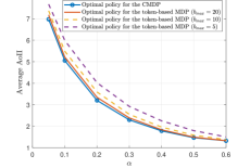
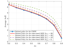
We compare the results of the optimal policies for the primary CMDP problem (1), and the corresponding token-based MDP problem (3). The first policy is derived through the optimal threshold finder presented in [4], while the second policy is obtained using the RVIA algorithm. In Figs. (2) and (3) the average AoII for both policies is depicted for various sets of system parameters. The optimal average AoII for various values of α𝛼\alpha has been illustrated in Fig. 2, with pR=0.5subscript𝑝𝑅0.5p_{R}=0.5 and N=8𝑁8N=8. In this figure, we have modified the value of bmaxsubscript𝑏maxb_{\text{max}} from 555 to 202020. As evident, the optimal AoII for the token-based MDP problem converges to the optimal AoII of the main CMDP problem. In Fig. 3, the optimal average AoII for two policies is depicted as a function of pRsubscript𝑝𝑅p_{R}, for N=8𝑁8N=8 and α=0.1𝛼0.1\alpha=0.1. The optimal average AoII for the token-based policy converges to the optimal average AoII of the main CMDP problem as the value of bmaxsubscript𝑏maxb_{\text{max}} increases. In both figures, we considered Δmax=30subscriptΔmax30\Delta_{\text{max}}=30.

Refer to caption
Figure 2: Optimal average AoII for two policies vs. α𝛼\alpha in
the single rate constrained problem.
Refer to caption
Figure 3: Optimal average AoII for two policies vs. pRsubscript𝑝𝑅p_{R} in
the single rate constrained problem.

V-B Two Rate Constrained Problem

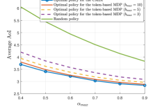
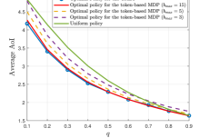
We compare the optimal token-based policy of the MDP problem (25) with the optimal policy derived from the primary CMDP problem (12), along with two additional baseline policies. We utilize the RVIA algorithm to solve the token-based MDP problem and the iterative triangle bisection algorithm to solve the CMDP problem. Subsequently, we compare the resulting average AoI for these two policies across various system parameters q𝑞q (Fig. 4) and αmaxsubscript𝛼max\alpha_{\text{max}} (Fig. 5), while keeping αminsubscript𝛼min\alpha_{\text{min}} fixed at 0.10.10.1. In Figs. 4 and 5, we also present the average AoI resulting from a uniform two-rate policy and a random policy. By a uniform two-rate policy, we mean that when r=0𝑟0r=0, the system is updated at a rate of αminsubscript𝛼min\alpha_{\text{min}}, and when r=1𝑟1r=1, the system is updated at a rate of αmaxsubscript𝛼max\alpha_{\text{max}}. Whereas, according to a random policy, the system is updated with probability αminsubscript𝛼min\alpha_{\text{min}} (αmaxsubscript𝛼max\alpha_{\text{max}}) when r=0𝑟0r=0 (r=1𝑟1r=1). ΔmaxsubscriptΔmax\Delta_{\text{max}}, ε𝝀subscript𝜀𝝀\varepsilon_{\bm{\lambda}}, and εVsubscript𝜀𝑉\varepsilon_{V} have been set to 202020, 0.10.10.1, and 0.10.10.1, respectively. The results are summarized as follows:

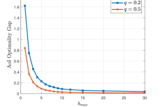
  • With an increase in bmaxsubscript𝑏maxb_{\text{max}}, the optimal average AoI for the token-based MDP problem converges to that of the primary CMDP problem. For further illustration, in Fig. 6, we plot the optimality gap between the token-based policy and the optimal policy for the main CMDP problem as a function of bmaxsubscript𝑏maxb_{\text{max}}, where αmax=0.5subscript𝛼max0.5\alpha_{\text{max}}=0.5 and q𝑞q is either 0.20.20.2 or 0.50.50.5.

  • Even for low levels of bmaxsubscript𝑏maxb_{\text{max}} (e.g. bmax=5subscript𝑏max5b_{\text{max}}=5), the performance of the optimal token-based policy is close to the optimal CMDP policy, and it outperforms both the uniform and random policies. In Section IV-D, we observed that when bmaxsubscript𝑏maxb_{\text{max}} is low, the RVIA’s complexity in finding the optimal token-based policy may be preferable to the iterative approach for the primary CMDP. This is particularly significant because the token-based approach offers a straightforward formulation and solution without becoming entangled in the Lagrangian formulation and the intricate aspects of the iterative bisection algorithm for the primary CMDP problem.
Refer to caption
Figure 4: Average AoI for different policies vs. q𝑞q (αmax=0.5subscript𝛼max0.5\alpha_{\text{max}}=0.5) in
the two rate constrained problem.
Refer to caption
Figure 5: Average AoI for different policies vs. αmaxsubscript𝛼max\alpha_{\text{max}} (q=0.2𝑞0.2q=0.2) in
the two rate constrained problem.
Refer to caption
Figure 6: Optimality gap vs. bmaxsubscript𝑏maxb_{\text{max}} in the two rate constrained problem.

VI Conclusion

In this work, we explored a token-based approach for transforming CMDP problems into unconstrained MDP problems, explicitly focusing on optimizing information freshness in status update systems. We have applied this approach to systems with one and two update rate constraints and examined the analytical structure of the optimal token-based policy. Additionally, we have introduced an iterative triangle bisection algorithm for solving CMDP problems with two constraints. Our findings demonstrate the superior performance of the optimal policy compared to baseline policies and the convergence of the optimal token-based policy to the optimal policy of the main CMDP problem as the maximum number of tokens in the system increases.

References

  • [1] S. Kaul, R. Yates, and M. Gruteser, “Real-time status: How often should one update?” in IEEE INFOCOM, March 2012.
  • [2] M. A. Abd-Elmagid, N. Pappas, and H. S. Dhillon, “On the role of age of information in the internet of things,” IEEE Communications Magazine, vol. 57, no. 12, 2019.
  • [3] N. Pappas, M. A. Abd-Elmagid, B. Zhou, W. Saad, and H. S. Dhillon, Age of Information: Foundations and Applications.   Cambridge University Press, 2023.
  • [4] A. Maatouk, S. Kriouile, M. Assaad, and A. Ephremides, “The age of incorrect information: A new performance metric for status updates,” IEEE/ACM Trans. on Networking, vol. 28, no. 5, 2020.
  • [5] R. D. Yates, “The age of gossip in networks,” in IEEE ISIT, 2021.
  • [6] A. Nikkhah, A. Ephremides, and N. Pappas, “Age of actuation in a wireless power transfer system,” in IEEE INFOCOM Workshops, 2023.
  • [7] E. T. Ceran, D. Gündüz, and A. György, “Average age of information with hybrid arq under a resource constraint,” IEEE Trans. on Wireless Communications, vol. 18, no. 3, 2019.
  • [8] Q. Wang, H. Chen, Y. Li, Z. Pang, and B. Vucetic, “Minimizing age of information for real-time monitoring in resource-constrained industrial iot networks,” in IEEE 17th INDIN, vol. 1, 2019.
  • [9] H. Tang, J. Wang, L. Song, and J. Song, “Minimizing age of information with power constraints: Multi-user opportunistic scheduling in multi-state time-varying channels,” IEEE Journal on Selected Areas in Communications, vol. 38, no. 5, 2020.
  • [10] G. Chen, Y. Chen, J. Wang, and J. Song, “Minimizing age of information in downlink wireless networks with time-varying channels and peak power constraint,” IEEE Trans. on Vehicular Technology, 2023.
  • [11] M. Hatami, M. Leinonen, Z. Chen, N. Pappas, and M. Codreanu, “On-demand aoi minimization in resource-constrained cache-enabled iot networks with energy harvesting sensors,” IEEE Trans. on Communications, vol. 70, no. 11, 2022.
  • [12] E. Altman, Constrained Markov decision processes.   Vol. 7, CRC Press, 1999.
  • [13] G. J. Stamatakis, O. Simeone, and N. Pappas, “Optimizing information freshness over a channel that wears out,” 57th Asilomar Conference on Signals, Systems, and Computers, 2023.
  • [14] A. S. Tanenbaum and D. J. Wetherall, Computer Networks, 2011.
  • [15] V. Raghunathan, S. Ganeriwal, M. Srivastava, and C. Schurgers, “Energy efficient wireless packet scheduling and fair queuing,” ACM Trans. on Embedded Computing Systems (TECS), vol. 3, no. 1, 2004.
  • [16] F. Chiariotti, J. Holm, A. E. Kalør, B. Soret, S. K. Jensen, T. B. Pedersen, and P. Popovski, “Query age of information: Freshness in pull-based communication,” IEEE Trans. on Communications, vol. 70, no. 3, 2022.
  • [17] R. D. Yates, “Lazy is timely: Status updates by an energy harvesting source,” in IEEE ISIT, 2015.
  • [18] B. T. Bacinoglu and E. Uysal-Biyikoglu, “Scheduling status updates to minimize age of information with an energy harvesting sensor,” in IEEE ISIT, 2017.
  • [19] G. Stamatakis, N. Pappas, and A. Traganitis, “Control of status updates for energy harvesting devices that monitor processes with alarms,” in IEEE Globecom Workshops, 2019.
  • [20] Z. Chen, N. Pappas, E. Björnson, and E. G. Larsson, “Optimizing information freshness in a multiple access channel with heterogeneous devices,” IEEE Open Journal of the Commun. Society, vol. 2, 2021.
  • [21] E. Gindullina, L. Badia, and D. Gündüz, “Age-of-information with information source diversity in an energy harvesting system,” IEEE Trans. on Green Communications and Networking, vol. 5, no. 3, 2021.
  • [22] M. Hatami, M. Leinonen, and M. Codreanu, “Aoi minimization in status update control with energy harvesting sensors,” IEEE Trans. on Communications, vol. 69, no. 12, 2021.
  • [23] E. Delfani and N. Pappas, “Version age-optimal cached status updates in a gossiping network with energy harvesting sensor,” in WiOpt, 2023.
  • [24] P. Agheli, N. Pappas, P. Popovski, and M. Kountouris, “Effective communication: When to pull updates?” in IEEE ICC, 2024.
  • [25] G. Stamatakis, N. Pappas, A. Fragkiadakis, N. Petroulakis, and A. Traganitis, “Semantics-aware active fault detection in status updating systems,” IEEE Open Journal of the Commun. Society, 2024.
  • [26] D. P. Bertsekas, Dynamic Programming and Optimal Control, Vol. II, 3rd ed.   Athena Scientific, 2007.
  • [27] F. J. Beutler and K. W. Ross, “Optimal policies for controlled markov chains with a constraint,” Journal of mathematical analysis and applications, vol. 112, no. 1, 1985.
  • [28] C. Harvey and F. Stenger, “A two-dimensional analogue to the method of bisections for solving nonlinear equations,” Quarterly of Applied Mathematics, vol. 33, no. 4, 1976.

Appendix A Proof of Theorem 1

Proof.

The Bellman equation at state s=(b,Δ)𝑠𝑏Δs\!=\!\left(b,\Delta\right) can be simplified as follows:

J+V(s)superscript𝐽𝑉𝑠\displaystyle J^{\ast}+V(s) =Δ+mina{0,1}{sSP[s|s,a]V(s)}.absentΔsubscript𝑎01subscriptsuperscript𝑠𝑆𝑃delimited-[]conditionalsuperscript𝑠𝑠𝑎𝑉superscript𝑠\displaystyle=\Delta+\min_{a\in\left\{0,1\right\}}{\left\{\sum_{s^{\prime}\in S}P\left[s^{\prime}|s,a\right]V(s^{\prime})\right\}}. (28)

Therefore, the optimal action can be obtained by:

a(s)=argmina{0,1}{sSP[s|s,a]V(s)}={0,DV(s)0,1,DV(s)<0,superscript𝑎𝑠subscriptargmin𝑎01subscriptsuperscript𝑠𝑆𝑃delimited-[]conditionalsuperscript𝑠𝑠𝑎𝑉superscript𝑠cases0𝐷𝑉𝑠01𝐷𝑉𝑠0\displaystyle a^{\ast}(s)\!=\!\operatorname*{arg\,min}_{a\in\left\{0,1\right\}}{\left\{\sum_{s^{\prime}\in S}\!P\left[s^{\prime}|s,a\right]V(s^{\prime})\right\}}\!=\!\begin{cases}0,&DV(s)\!\geq\!0,\\ 1,&DV(s)\!<\!0,\\ \end{cases}

where V0(s)=defsSP[s|s,a=0]V(s)superscript𝑉0𝑠defsubscriptsuperscript𝑠𝑆𝑃delimited-[]conditionalsuperscript𝑠𝑠𝑎0𝑉superscript𝑠V^{0}(s)\overset{\text{def}}{\!=\!}\sum_{s^{\prime}\in S}P\left[s^{\prime}|s,a\!=\!0\right]V(s^{\prime}), V1(s)=defsSP[s|s,a=1]V(s)superscript𝑉1𝑠defsubscriptsuperscript𝑠𝑆𝑃delimited-[]conditionalsuperscript𝑠𝑠𝑎1𝑉superscript𝑠V^{1}(s)\overset{\text{def}}{\!=\!}\sum_{s^{\prime}\in S}\!P\left[s^{\prime}|s,a\!=\!1\right]V(s^{\prime}), and DV(s)=defV1(s)V0(s)𝐷𝑉𝑠defsuperscript𝑉1𝑠superscript𝑉0𝑠DV(s)\!\overset{\text{def}}{=}\!V^{1}(s)\!-\!V^{0}(s).

As can be seen, the optimal action a(s)superscript𝑎𝑠a^{\ast}(s) is related to the sign of DV(s)𝐷𝑉𝑠DV(s). When b=0𝑏0b=0 or Δ=0Δ0\Delta=0, it can be simply shown that DV(s)=0𝐷𝑉𝑠0DV(s)=0; thus the action a=0𝑎0a=0 is optimal. For other cases where b>0𝑏0b>0 and Δ>0Δ0\Delta>0, we have:

V0(s)superscript𝑉0𝑠\displaystyle V^{0}(s) =αptV(b+1,0)+α(1pt)V(b+1,Δ+1)absent𝛼subscript𝑝𝑡𝑉𝑏10𝛼1subscript𝑝𝑡𝑉𝑏1Δ1\displaystyle\!=\!\alpha p_{t}V(b\!+\!1,0)\!+\!\alpha\left(1\!-\!p_{t}\right)V(b\!+\!1,\Delta\!+\!1) (29a)
+(1α)ptV(b,0)+(1α)(1pt)V(b,Δ+1),1𝛼subscript𝑝𝑡𝑉𝑏01𝛼1subscript𝑝𝑡𝑉𝑏Δ1\displaystyle+(1-\alpha)p_{t}V(b,0)+(1-\alpha)\left(1-p_{t}\right)V(b,\Delta+1),
V1(s)superscript𝑉1𝑠\displaystyle V^{1}(s) =αβV(b,0)+α(1β)V(b,Δ+1)absent𝛼𝛽𝑉𝑏0𝛼1𝛽𝑉𝑏Δ1\displaystyle=\alpha\beta V(b,0)+\alpha\left(1-\beta\right)V(b,\Delta+1) (29b)
+(1α)βV(b1,0)+(1α)(1β)V(b1,Δ+1),1𝛼𝛽𝑉𝑏101𝛼1𝛽𝑉𝑏1Δ1\displaystyle+(1\!-\!\alpha)\beta V(b\!-\!1,0)+(1\!-\!\alpha)\left(1\!-\!\beta\right)V(b\!-\!1,\Delta\!+\!1),

In what follows, we demonstrate that DV(s)=DV(b,Δ)=V1(s)V0(s)𝐷𝑉𝑠𝐷𝑉𝑏Δsuperscript𝑉1𝑠superscript𝑉0𝑠DV(s)=DV(b,\Delta)=V^{1}(s)-V^{0}(s) is a decreasing function of ΔΔ\Delta, i.e., for ΔΔ+superscriptΔsuperscriptΔ\Delta\!^{-}\leq\Delta\!^{+}, we show that DV(b,Δ+)DV(b,Δ)𝐷𝑉𝑏superscriptΔ𝐷𝑉𝑏superscriptΔDV(b,\Delta\!^{+})\leq DV(b,\Delta\!^{-}) or DV(b,Δ+)DV(b,Δ)0𝐷𝑉𝑏superscriptΔ𝐷𝑉𝑏superscriptΔ0DV(b,\Delta\!^{+})-DV(b,\Delta\!^{-})\leq 0. By simplification of DV(b,Δ+)𝐷𝑉𝑏superscriptΔDV(b,\Delta\!^{+}) and DV(b,Δ)𝐷𝑉𝑏superscriptΔDV(b,\Delta\!^{-}) based on (29) we obtain:

DV(b,Δ+)DV(b,Δ)𝐷𝑉𝑏superscriptΔ𝐷𝑉𝑏superscriptΔ\displaystyle DV(b,\Delta\!^{+})-DV(b,\Delta\!^{-})
=α{(1β)[V(b,Δ++1)V(b,Δ+1)]\displaystyle=\alpha\Big{\{}(1\!-\!\beta)\big{[}V(b,\Delta\!^{+}\!+\!1)\!-\!V(b,\Delta\!^{-}\!+\!1)\big{]}
(1pt)[V(b+1,Δ++1)V(b+1,Δ+1)]}\displaystyle\quad-\!(1\!-\!p_{t})\big{[}V(b\!+\!1,\Delta\!^{+}\!+\!1)\!-\!V(b\!+\!1,\Delta\!^{-}\!+\!1)\big{]}\Big{\}}
+(1α){(1β)[V(b1,Δ++1)V(b1,Δ+1)]\displaystyle\quad+(1\!-\!\alpha)\Big{\{}(1\!-\!\beta)\big{[}V(b\!-\!1,\Delta\!^{+}\!+\!1)\!-\!V(b\!-\!1,\Delta\!^{-}\!+\!1)\big{]}
(1pt)[V(b,Δ++1)V(b,Δ+1)]}.\displaystyle\quad-\!(1\!-\!p_{t})\big{[}V(b,\Delta\!^{+}\!+\!1)\!-\!V(b,\Delta\!^{-}\!+\!1)\big{]}\Big{\}}. (30)

According to (A), to confirm the inequality DV(b,Δ+)DV(b,Δ)0𝐷𝑉𝑏superscriptΔ𝐷𝑉𝑏superscriptΔ0DV(b,\Delta\!^{+})-DV(b,\Delta\!^{-})\leq 0, it suffice to demonstrate that (1β)[V(b1,Δ+)V(b1,Δ)](1pt)[V(b,Δ+)V(b,Δ)]01𝛽delimited-[]𝑉𝑏1superscriptΔ𝑉𝑏1superscriptΔ1subscript𝑝𝑡delimited-[]𝑉𝑏superscriptΔ𝑉𝑏superscriptΔ0(1-\beta)\big{[}V(b-1,\Delta\!^{+})-V(b-1,\Delta\!^{-})\big{]}-(1-p_{t})\big{[}V(b,\Delta\!^{+})-V(b,\Delta\!^{-})\big{]}\leq 0, for b>0𝑏0b>0 and 1<ΔΔ+1superscriptΔsuperscriptΔ1<\Delta\!^{-}\leq\Delta\!^{+}. We utilize the VIA and mathematical induction to proceed with the proof. VIA converges to the value function of Bellman’s equation irrespective of the initial value assigned to V0(s)subscript𝑉0𝑠V_{0}(s), i.e., limkVk(s)=V(s)sSsubscript𝑘subscript𝑉𝑘𝑠𝑉𝑠for-all𝑠𝑆\lim_{k\rightarrow\infty}{V_{k}(s)}=V(s)\ \forall s\in S. Therefore, it suffices to establish the following inequality for all k{0,1,2,}𝑘012k\in\{0,1,2,\cdots\}:

(1β)[Vk(b1,Δ+)Vk(b1,Δ)](1pt)[Vk(b,Δ+)Vk(b,Δ)]0.1𝛽delimited-[]subscript𝑉𝑘𝑏1superscriptΔsubscript𝑉𝑘𝑏1superscriptΔ1subscript𝑝𝑡delimited-[]subscript𝑉𝑘𝑏superscriptΔsubscript𝑉𝑘𝑏superscriptΔ0(1-\beta)\big{[}V_{k}(b\!-\!1,\Delta\!^{+})\!-\!V_{k}(b\!-\!1,\Delta\!^{-})\big{]}\\ \!-\!(1\!-\!p_{t})\big{[}V_{k}(b,\Delta\!^{+})\!-\!V_{k}(b,\Delta\!^{-})\big{]}\leq 0. (31)

Assuming V0(s)=0subscript𝑉0𝑠0V_{0}(s)=0 for all sS𝑠𝑆s\in S, (31) holds true for k=0𝑘0k=0. Now, with the same assumption extending up to k>0𝑘0k>0, we prove its validity for k+1𝑘1k+1. By defining Vk+10(s)=sSP[s|s,a=0]Vk(s)subscriptsuperscript𝑉0𝑘1𝑠subscriptsuperscript𝑠𝑆𝑃delimited-[]conditionalsuperscript𝑠𝑠𝑎0subscript𝑉𝑘superscript𝑠V^{0}_{k+1}(s)=\sum_{s^{\prime}\in S}P\left[s^{\prime}|s,a=0\right]V_{k}(s^{\prime}), Vk+11(s)=sSP[s|s,a=1]Vk(s)subscriptsuperscript𝑉1𝑘1𝑠subscriptsuperscript𝑠𝑆𝑃delimited-[]conditionalsuperscript𝑠𝑠𝑎1subscript𝑉𝑘superscript𝑠V^{1}_{k+1}(s)\!=\!\sum_{s^{\prime}\in S}\!P\left[s^{\prime}|s,a\!=\!1\right]V_{k}(s^{\prime}),

V𝑉\displaystyle V (s)k+10=αptVk(b+1,0)+α(1pt)Vk(b+1,Δ+1){}^{0}_{k+1}(s)=\alpha p_{t}V_{k}(b\!+\!1,0)+\alpha\left(1\!-\!p_{t}\right)V_{k}(b\!+\!1,\Delta\!+\!1)
+(1α)ptVk(b,0)+(1α)(1pt)Vk(b,Δ+1),1𝛼subscript𝑝𝑡subscript𝑉𝑘𝑏01𝛼1subscript𝑝𝑡subscript𝑉𝑘𝑏Δ1\displaystyle+(1\!-\!\alpha)p_{t}V_{k}(b,0)+(1\!-\!\alpha)\left(1\!-\!p_{t}\right)V_{k}(b,\Delta\!+\!1), (32a)
V𝑉\displaystyle V (s)k+11=αβVk(b,0)+α(1β)Vk(b,Δ+1){}^{1}_{k+1}(s)=\alpha\beta V_{k}(b,0)+\alpha\left(1\!-\!\beta\right)V_{k}(b,\Delta\!+\!1) (32b)
+(1α)βVk(b1,0)+(1α)(1β)Vk(b1,Δ+1),1𝛼𝛽subscript𝑉𝑘𝑏101𝛼1𝛽subscript𝑉𝑘𝑏1Δ1\displaystyle+(1\!-\!\alpha)\beta V_{k}(b\!-\!1,0)+(1\!-\!\alpha)\left(1\!-\!\beta\right)V_{k}(b\!-\!1,\Delta\!+\!1),

the VIA equation is given by Vk+1(b,Δ)=Δ+min{Vk+10(b,Δ),Vk+11(b,Δ)}subscript𝑉𝑘1𝑏ΔΔsubscriptsuperscript𝑉0𝑘1𝑏Δsubscriptsuperscript𝑉1𝑘1𝑏ΔV_{k+1}(b,\Delta)=\Delta+\min\{V^{0}_{k+1}(b,\Delta),V^{1}_{k+1}(b,\Delta)\}; thus the inequality (31) for k+1𝑘1k+1 can further be simplified:

(ptβ)<0(Δ+Δ)0subscriptsubscript𝑝𝑡𝛽absent0subscriptsuperscriptΔsuperscriptΔabsent0\displaystyle\underbrace{(p_{t}-\beta)}_{<0}\underbrace{(\Delta\!^{+}-\Delta\!^{-})}_{\geq 0}
+(1β)[min{Vk+10(b1,Δ+),Vk+11(b1,Δ+)}\displaystyle+(1-\beta)\Big{[}\min\{V^{0}_{k+1}(b-1,\Delta\!^{+}),V^{1}_{k+1}(b-1,\Delta\!^{+})\}
min{Vk+10(b1,Δ),Vk+11(b1,Δ)}]\displaystyle\qquad\qquad-\min\{V^{0}_{k+1}(b-1,\Delta\!^{-}),V^{1}_{k+1}(b-1,\Delta\!^{-})\}\Big{]}
(1pt)[min{Vk+10(b,Δ+),Vk+11(b,Δ+)}\displaystyle-(1-p_{t})\Big{[}\min\{V^{0}_{k+1}(b,\Delta\!^{+}),V^{1}_{k+1}(b,\Delta\!^{+})\}
min{Vk+10(b,Δ),Vk+11(b,Δ)}]0.\displaystyle\qquad\qquad-\min\{V^{0}_{k+1}(b,\Delta\!^{-}),V^{1}_{k+1}(b,\Delta\!^{-})\}\Big{]}\leq 0. (33)

The first term in (A) is non-positive; thus, it is sufficient to demonstrate that the other terms, which we denote by E1subscript𝐸1E_{1}, are non-positive, i.e., E10subscript𝐸10E_{1}\leq 0. To proceed with the proof, we consider four cases. Case 1, where Vk+10(b1,Δ)Vk+11(b1,Δ)subscriptsuperscript𝑉0𝑘1𝑏1superscriptΔsubscriptsuperscript𝑉1𝑘1𝑏1superscriptΔV^{0}_{k+1}(b-1,\Delta\!^{-})\leq V^{1}_{k+1}(b-1,\Delta\!^{-}) and Vk+10(b,Δ+)Vk+11(b,Δ+)subscriptsuperscript𝑉0𝑘1𝑏superscriptΔsubscriptsuperscript𝑉1𝑘1𝑏superscriptΔV^{0}_{k+1}(b,\Delta\!^{+})\leq V^{1}_{k+1}(b,\Delta\!^{+}); case 2, where Vk+10(b1,Δ)Vk+11(b1,Δ)subscriptsuperscript𝑉0𝑘1𝑏1superscriptΔsubscriptsuperscript𝑉1𝑘1𝑏1superscriptΔV^{0}_{k+1}(b-1,\Delta\!^{-})\leq V^{1}_{k+1}(b-1,\Delta\!^{-}) and Vk+10(b,Δ+)>Vk+11(b,Δ+)subscriptsuperscript𝑉0𝑘1𝑏superscriptΔsubscriptsuperscript𝑉1𝑘1𝑏superscriptΔV^{0}_{k+1}(b,\Delta\!^{+})>V^{1}_{k+1}(b,\Delta\!^{+}); cases 3 and 4 are defined by reversing the inequality signs in cases 1 and 2. We prove the inequality E10subscript𝐸10E_{1}\leq 0 for case 1; a similar approach can be utilized to prove the other cases. In this case, equation E10subscript𝐸10E_{1}\leq 0 is simplified:

(1β)[min{Vk+10(b1,Δ+),Vk+11(b1,Δ+)}Vk+10(b1,Δ)]1𝛽delimited-[]subscriptsuperscript𝑉0𝑘1𝑏1superscriptΔsubscriptsuperscript𝑉1𝑘1𝑏1superscriptΔsubscriptsuperscript𝑉0𝑘1𝑏1superscriptΔ\displaystyle(1\!-\!\beta)\Big{[}\min\{V^{0}_{k+1}(b\!-\!1,\Delta\!^{+}),V^{1}_{k+1}(b\!-\!1,\Delta\!^{+})\}\!-\!V^{0}_{k+1}(b\!-\!1,\Delta\!^{-})\Big{]}
(1pt)[Vk+10(b,Δ+)min{Vk+10(b,Δ),Vk+11(b,Δ)}]01subscript𝑝𝑡delimited-[]subscriptsuperscript𝑉0𝑘1𝑏superscriptΔsubscriptsuperscript𝑉0𝑘1𝑏superscriptΔsubscriptsuperscript𝑉1𝑘1𝑏superscriptΔ0\displaystyle\quad-(1\!-\!p_{t})\Big{[}V^{0}_{k+1}(b,\Delta\!^{+})\!-\!\min\{V^{0}_{k+1}(b,\Delta\!^{-}),V^{1}_{k+1}(b,\Delta\!^{-})\}\Big{]}\leq 0
(a)(1β)[Vk+10(b1,Δ+)Vk+10(b1,Δ)]𝑎1𝛽delimited-[]subscriptsuperscript𝑉0𝑘1𝑏1superscriptΔsubscriptsuperscript𝑉0𝑘1𝑏1superscriptΔ\displaystyle\underset{(a)}{\Leftrightarrow}(1\!-\!\beta)\Big{[}V^{0}_{k+1}(b\!-\!1,\Delta\!^{+})\!-\!V^{0}_{k+1}(b\!-\!1,\Delta\!^{-})\Big{]}\!
+(1β)min{0,Vk+11(b1,Δ+)Vk+10(b1,Δ+)}1𝛽0subscriptsuperscript𝑉1𝑘1𝑏1superscriptΔsubscriptsuperscript𝑉0𝑘1𝑏1superscriptΔ\displaystyle\qquad+\!(1\!-\!\beta)\min\{0,V^{1}_{k+1}(b\!-\!1,\Delta\!^{+})\!-\!V^{0}_{k+1}(b\!-\!1,\Delta\!^{+})\}
(1pt)[Vk+10(b,Δ+)Vk+10(b,Δ)]1subscript𝑝𝑡delimited-[]subscriptsuperscript𝑉0𝑘1𝑏superscriptΔsubscriptsuperscript𝑉0𝑘1𝑏superscriptΔ\displaystyle\qquad-(1\!-\!p_{t})\Big{[}V^{0}_{k+1}(b,\Delta\!^{+})\!-\!V^{0}_{k+1}(b,\Delta\!^{-})\Big{]}
+(1pt)min{0,Vk+11(b,Δ)Vk+10(b,Δ)}0,1subscript𝑝𝑡0subscriptsuperscript𝑉1𝑘1𝑏superscriptΔsubscriptsuperscript𝑉0𝑘1𝑏superscriptΔ0\displaystyle\qquad+(1\!-\!p_{t})\min\{0,V^{1}_{k+1}(b,\Delta\!^{-})\!-\!V^{0}_{k+1}(b,\Delta\!^{-})\}\leq 0, (34)

where (a)𝑎(a) is resulted from min{x,y}=x+min{0,yx}𝑥𝑦𝑥0𝑦𝑥\min\left\{x,y\right\}=x+\min\left\{0,y-x\right\}. Since the second and last terms are negative (non-positive), it suffices to show that:

(1β)[Vk+10(b1,Δ+)Vk+10(b1,Δ)](1pt)[Vk+10(b,Δ+)Vk+10(b,Δ)]0,1𝛽delimited-[]subscriptsuperscript𝑉0𝑘1𝑏1superscriptΔsubscriptsuperscript𝑉0𝑘1𝑏1superscriptΔ1subscript𝑝𝑡delimited-[]subscriptsuperscript𝑉0𝑘1𝑏superscriptΔsubscriptsuperscript𝑉0𝑘1𝑏superscriptΔ0(1-\beta)\Big{[}V^{0}_{k+1}(b-1,\Delta\!^{+})-V^{0}_{k+1}(b-1,\Delta\!^{-})\Big{]}\\ -(1-p_{t})\Big{[}V^{0}_{k+1}(b,\Delta\!^{+})-V^{0}_{k+1}(b,\Delta\!^{-})\Big{]}\leq 0, (35)

where, according to (32) and after some manipulation, it can be expressed as follows:

α(1pt){(1β)[Vk(b,Δ++1)Vk(b,Δ+1)]\displaystyle\alpha\left(1\!-\!p_{t}\right)\Big{\{}(1\!-\!\beta)\big{[}V_{k}(b,\Delta\!^{+}\!+\!1)\!-\!V_{k}(b,\Delta\!^{-}\!+\!1)\big{]}
(1pt)[Vk(b+1,Δ++1)Vk(b+1,Δ+1)]}\displaystyle-\!(1\!-\!p_{t})\big{[}V_{k}(b\!+\!1,\Delta\!^{+}\!+\!1)\!-\!V_{k}(b\!+\!1,\Delta\!^{-}\!+\!1)\big{]}\Big{\}}
+(1α)(1pt){(1β)[Vk(b1,Δ++1)Vk(b1,Δ+1)]\displaystyle+\!(1\!-\!\alpha)\!\left(1\!-\!p_{t}\right)\!\Big{\{}\!(1\!-\!\beta)\big{[}\!V_{k}(b\!-\!1,\Delta\!^{+}\!+\!1)\!-\!V_{k}(b\!-\!1,\Delta\!^{-}\!+\!1)\big{]}
(1pt)[Vk(b,Δ++1)Vk(b,Δ+1)]}0,\displaystyle-\!(1\!-\!p_{t})\big{[}V_{k}(b,\Delta\!^{+}\!+\!1)\!-\!V_{k}(b,\Delta\!^{-}\!+\!1)\big{]}\Big{\}}\leq 0, (36)

where both the expressions within the braces are negative according to (31), and the proof is complete. ∎