Federated Learning for Cooperative Inference Systems: The Case of Early Exit Networks

Abstract

As Internet of Things (IoT) technology advances, end devices like sensors and smartphones are progressively equipped with AI models tailored to their local memory and computational constraints. Local inference reduces communication costs and latency; however, these smaller models typically underperform compared to more sophisticated models deployed on edge servers or in the cloud. Cooperative Inference Systems (CISs) address this performance trade-off by enabling smaller devices to offload part of their inference tasks to more capable devices. These systems often deploy hierarchical models that share numerous parameters, exemplified by Deep Neural Networks (DNNs) that utilize strategies like early exits or ordered dropout. In such instances, Federated Learning (FL) may be employed to jointly train the models within a CIS. Yet, traditional training methods have overlooked the operational dynamics of CISs during inference, particularly the potential high heterogeneity in serving rates across clients. To address this gap, we propose a novel FL approach designed explicitly for use in CISs that accounts for these variations in serving rates. Our framework not only offers rigorous theoretical guarantees, but also surpasses state-of-the-art (SOTA) training algorithms for CISs, especially in scenarios where inference request rates or data availability are uneven among clients.

2911

1 Introduction

The integration of intelligent capabilities into devices such as sensors, smartphones, and IoT equipment is becoming increasingly critical [36, 35]. However, a significant hurdle in this field is the resource heterogeneity within real-world networks, where clients often have varying memory and computational capacities. This disparity makes it infeasible to deploy a uniform AI model across all network nodes [9, 17]. To address this issue, Cooperative Inference Systems (CISs) have been developed. These systems allow less capable devices to offload parts of their inference tasks to more powerful devices within the network, thereby leveraging other available AI models to enhance overall performance [31, 27].

Most research on CISs assumes the availability of such AI models and primarily focuses on either optimizing their placement within a network and/or identifying a beneficial cooperative serving policy [11, 40, 31, 27]. Significantly less research has focused on the training methodologies for deploying heterogeneous models within a CIS. This paper specifically explores scenarios in which models are collaboratively trained using distributed datasets, hosted on the very clients that subsequently perform inference tasks.

Federated learning (FL) [23, 9, 13] is a framework that facilitates collaborative model training across clients without necessitating the sharing of local data, and can enable knowledge transfer among heterogeneous models through either explicit knowledge distillation—typically requiring a public dataset [18, 25]—or by mandating that the models share a subset of parameters. Within this latter approach, prevalent methods include the joint training of Deep Neural Networks (DNNs) that either share entire layers or specific parameters within a layer. This can be achieved through techniques such as ordered dropout [3, 5] or early exits [33, 34]. The final configuration of these shared parameters is influenced by the diverse and potentially conflicting requirements of the different models. For instance, parameters within a shared layer may learn to identify features of varying complexity depending on whether the layer is part of a deeper or shallower DNN.

It may seem natural to balance these conflicting requirements by considering the role of each model within the CIS at inference time. For instance, one might expect that models expected to handle a greater volume of inference requests should exert a more substantial influence on the final tuning of the shared parameters. Nevertheless, to the best of our knowledge, existing research has ignored these unique attributes of the CIS setting. For example, existing approaches such as those proposed in [34, 26, 8] for training distributed early-exit networks assign equal importance to all models.

This paper represents the first effort to introduce a more principled approach to FL training of models in a CIS. Our methodology aims to systematically address the distinctive challenges posed by CISs, filling a critical gap in the current literature.

Contributions.

Our first contribution is the formulation of CIS training under realistic inference service constraints as an opportune optimization problem. We demonstrate that, under a reasonable assumption, this problem can be transformed into an equivalent simpler optimization problem. Here, the objective function (the true error) is a weighted sum of the expected losses for each trained model, with weights $\bm{\Lambda}$ corresponding to the expected inference request rates.

Our second contribution is the proposal of a general FL algorithm designed to minimize an opportune weighted sum of empirical losses over the clients. This algorithm enables computationally stronger clients to assist weaker clients in model training according to predefined probabilities. It functions by integrating two sets of parameters: the weights of the empirical losses $\bm{\tilde{\Lambda}}$ (which may differ from $\bm{\Lambda}$), and the probabilities matrix $\bm{p}$.

Our third contribution is a rigorous analysis of the impact of the key parameters $\bm{\tilde{\Lambda}}$ and $\bm{p}$ on the true error. We dissect the error into its constituent components—generalization error, bias error, and optimization error—to provide a comprehensive understanding of how these parameters influence the training process and the corresponding tradeoffs, and to derive practical configuration guidelines.

Finally, we present experimental results that demonstrate that our approach significantly outperforms state-of-the-art methods, particularly in scenarios characterized by uneven inference request rates or data availability among clients.

Outline of Paper.

The paper is organized as follows. Section 2 provides relevant background. Section 3 formalizes the model training problem in a CIS and introduces our novel FL algorithm. We present the theoretical guarantees of our approach in Section 3.3. Section 4 evaluates our algorithm against state-of-the-art (SOTA) training methods for early exit networks in a CIS setting. Finally, Section 5 concludes the paper and explores potential avenues for future work.

2 Background and Related Work

2.1 Cooperative Inference Systems

A Cooperative Inference Systems (CIS), also known in the literature as collaborative inference systems [27] or inference delivery networks [31], represent a dynamic field of study. The scope of collaboration in these systems may vary, extending beyond the traditional device-cloud model to include intermediate nodes such as edge servers, regional clouds, or a collective of devices within direct transmission range of each other [27, 34, 11, 40, 31]. The form of cooperation within a CIS can also significantly vary. For example, nodes in a CIS may run different parts of the same model according to the split computing framework [22]. Alternatively, they may integrate the predictions of various models in an ensemble approach [20, 39], thereby enhancing the robustness and accuracy of the inference. Furthermore, nodes might selectively forward their inference requests—particularly the more complex ones—to more powerful models within the network. In this paper, we study a generic hierarchy of nodes, each equipped with models of progressively higher complexity, that cooperate by forwarding requests.

While much previous work has concentrated on optimizing the deployment and utilization of already trained model in a CIS [11, 40, 31], our research shifts focus to the less-explored challenge of training these models in a FL context. Here, each CIS client utilizes its local dataset to contribute to the training of the set of models intended for deployment across the network.

2.2 Federated Learning for a CIS

Traditional algorithms for FL (e.g., FedAvg [23], FedProx [14]) assume that the participating clients have the same storage and computation capacities, i.e., every client holds a DNN of the same architecture and can perform the same amount of computation during training. More recently, new algorithms have been proposed to efficiently train multiple model of different sizes in a federated network. Federated distillation techniques [18] rely on a powerful orchestrator to distill knowledge across a limited number of different models. However, this approach requires the orchestrator to have access to a public dataset. More practical approaches rely on jointly training models that share a subset of the parameters. For example, Horvath et al. [5] propose a framework called FjORD, where a DNN is pruned by channels to generate nested submodels of different sizes that can fit into heterogeneous clients (following a mechanism referred to as ordered dropout). A similar idea can be also found in [3]. Alternative approaches involves the use of early exit networks [26] or a combination of these two methods [8]. While our algorithm and subsequent analysis are applicable to both pruning (e.g., ordered dropout) and early exit strategies, for clarity and concreteness, we have chosen to focus specifically on early exit networks. We provide a more detailed description of this approach in the following section.

2.3 Early Exit Networks

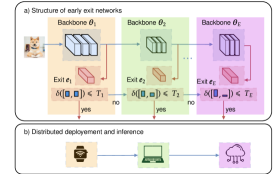
Figure 1: Cooperative Inference System with Early Exit Networks.

Early Exit Networks (EENs), introduced initially as BranchyNet [33], extend Deep Neural Networks (DNNs) by incorporating additional classifiers (i.e., early exits) at intermediate layers. For instance, integrating an early exit into a standard ResNet-34 [4] architecture might involve adding a classifier after the 18th layer, effectively enabling the original ResNet-34 to also function as a ResNet-18. The initial motivation for such a design is to allow for faster real-time inference with less computational cost, which is especially useful in computationally heavy computer vision and natural language processing tasks [22, Table 4]. As depicted in Figure 1(a), the process works as follows: during the inference for an input sample, if an early exit provides a high-confidence prediction (e.g., falling below a predefined entropy threshold), inference terminates immediately at that exit and the prediction is served. Otherwise, the sample is transmitted to the subsequent exit for processing. Within a CIS, the procedure can be extended to a distributed setting where each client maintains a model that includes a specific exit and all possible smaller exits. During inference, instead of transmitting the input sample within the same model from one exit to the next, the sample will be sent from a client on one layer of the network to a client on the subsequent layer that holds a more powerful exit as shown in Figure 1(b).

The most prevalent training strategy for EENs is to jointly train all the exits simultaneously, i.e.,  to minimize the expected weighted loss across all the exits [33, 7, 12, 6, 10]:

$$\min_{\boldsymbol{w}\in\mathbb{R}^{d}}\mathbb{E}_{z\sim{\mathcal{D}}}\left[\>\sum_{e=1}^{E}\alpha_{e}\>\ell^{(e)}(\bm{w},z)\right],$$ (1)

where the dataset sample $z=\left(x,y\right)$ is drawn from a data distribution ${\mathcal{D}}$, $x$ is the input features and $y$ is the target, $E$ denotes the total number of early exits, $\boldsymbol{w}$ denotes the parameters of the EEN, $\ell^{(e)}$ denotes the loss on the prediction given by early exit $e$, and $\alpha_{e}\in\mathbb{R}_{\geq 0}$ is the weight given to exit $e$. The weight coefficients $\alpha_{e}$ can be assigned in several ways. Common approaches include using constant equal weights for all exits [7, 34, 26, 8], manual tuning the weights for each exit [33, 10], or employing adaptive tuning techniques that adjust weights dynamically during training [12, 6].

3 Cooperative Inference System Using Federated Early Exit Networks

This section is organized as follows. In Sec. 3.1, we formalize the CIS and the training objective that takes into account inference requests. In Sec. 3.2, we present our algorithm for clients in a CIS to cooperatively train an EEN. In Sec. 3.3, we provide theoretical guarantees on the algorithm’s convergence errors.

3.1 Problem formulation

Network Topology.

Let $\mathcal{N}=\left\{1,2,\dots,N\right\}$ be the set of nodes in a CIS. The most common network topology in a CIS involves a rooted tree structure (e.g., cloud-edge-device structure [27]), where the parent nodes have bigger memory and higher computational capacity than the children nodes. For example, in Figure 2, client 1 represents the cloud, clients 2 and 3 represent the edges, and clients 4, 5, 6, and 7 represent devices.

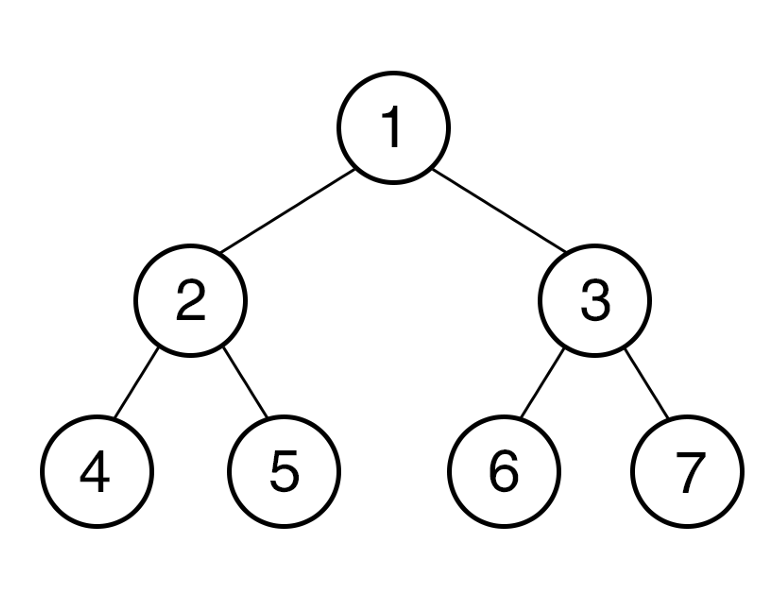
Figure 2: Example of network topology in CIS.

We denote $\mathcal{L}\subset\mathcal{N}$ to be the set of leaf nodes in the rooted tree and $\mathcal{N}^{-}_{i}$ the set of children of node $i\in\mathcal{N}$. For the case of training early exit networks, every node $i$ holds all exits from 1 up to $E_{i}$, where $E_{i}\leq E$ and $E_{i}>E_{j},\forall j\in\mathcal{N}^{-}_{i}$. Notice that, for inference, node $i$ only employs its largest available exit $E_{i}$, as it yields the most accurate prediction. We denote $\mathcal{N}_{e}$ to be the set of nodes that employ early exit $e$ for inference, i.e., $\mathcal{N}_{e}=\{i\in\mathcal{N}|E_{i}=e\}$.

Real-time Inference Requests.

Every node $i\in\mathcal{N}$ has local data arriving with a request rate $\lambda^{g}_{i}\in\mathbb{R}_{\geq 0}$. In a CIS, a child can forward an inference request to its parents (more capable nodes). Let $\lambda^{t}_{i}$ be the forwarding (transmission) rate of node $i$ to its parent. The total requests of a node $i$ is the sum of its requests forwarded by its children plus its local requests. Among these requests, node $i$ serves locally a fraction $f_{i}\in[0,1]$ of them using its inference model (e.g., early exit $E_{i}$ for the case of early exit networks). The rest of the requests are transmitted to its parent node. Let $\lambda^{s}_{i}$ be the serving rate of requests of node $i$. Thus, we have:

$$\textstyle\lambda^{s}_{i}\triangleq\left(\lambda^{g}_{i}+\sum_{j\in\mathcal{N}^{-}_{i}}\lambda^{t}_{j}\right)f_{i},$$ (2)

$$\lambda^{t}_{i}\triangleq\textstyle\left(\lambda^{g}_{i}+\sum_{j\in\mathcal{N}^{-}_{i}}\lambda^{t}_{j}\right)(1-f_{i}).$$ (3)

Note that the transmission rate $\lambda^{t}_{i}$ has an upper bound defined by the network budget (e.g., latency and bandwidth), which we denote $\mu^{\mathrm{max}}_{i}$. We assume that each node has access to its $\mu^{\mathrm{max}}_{i}$ and an estimate on its arrival rate $\lambda^{g}_{i}$. In addition, every node $i$ can rank samples according to their difficulty w.r.t some criterion [33, 7, 10], and it can select the $f_{i}$ fraction of its easiest samples to be served locally. Let $\mathcal{D}^{s}_{i}$ denote the data distribution of these served samples at node $i$.

Training objective for CIS.

To provide the best service in a CIS, one would expect that the final deployed models maximize the total inference quality, i.e., minimize the loss of all the served samples over all the nodes. With this objective in mind, we formalize the first inference-aware training framework for a CIS using an EEN, where the aim is to solve the following optimization problem w.r.t. the model parameters $\bm{w}$ and the serving fraction $\{f_{i},\forall i\in\mathcal{N}\}$.

$${\mathbb{P}}_{1}: \min_{\bm{w},\{f_{i}\}}\sum_{i\in\mathcal{N}}\mathbb{E}_{z\sim{\mathcal{D}}^{s}_{i}}\left[\ell^{(E_{i})}(\bm{w},z)\right]\lambda^{s}_{i},$$

s.t., $$\lambda^{t}_{i}\leq\mu^{\mathrm{max}}_{i},f_{i}\in[0,1],\quad \forall i\in\mathcal{N},$$ (4)

Eqs.2 and 3 $$\forall i\in\mathcal{N}.$$

Existing works [33, 1, 40] demonstrate that usually early exits later in the network result in better accuracy performance on the inference data. Based on this observation, in order to ensure the best quality of inference, smaller nodes are inclined to offload as many requests as possible to their parent nodes, thereby saturating the network budget condition (4). A contradiction illustrates this point: suppose in the optimal solution of ${\mathbb{P}}_{1}$, there exists a node with $f^{*}_{i}$ s.t. $\lambda^{t}_{i}<\mu^{\mathrm{max}}_{i}$. By decreasing $f^{*}_{i}$ to a value that makes $\lambda^{t}_{i}=\mu^{\mathrm{max}}_{i}$ and adjusting $f^{*}_{j}$ s.t. the parent node $j$ serves these additional requests locally, we achieve another feasible solution to ${\mathbb{P}}_{1}$ with a smaller loss.

Therefore, we can limit the search space to such strategies, and obtain the following simplified equivalent optimization problem:

$${\mathbb{P}}_{2}: \min_{\bm{w}}\sum_{e=1}^{E}\mathbb{E}_{z\sim{\hat{\mathcal{D}}}_{e}}\left[\ell^{(e)}(\bm{w},z)\right]\Lambda_{e},$$ (5)

where ${\hat{\mathcal{D}}}_{e}$ denotes the data distribution of serving samples at early exit $e$, $\Lambda_{e}=\sum_{i\in\mathcal{N}_{e}}\left(\lambda^{g}_{i}+\sum_{j\in\mathcal{N}^{-}_{i}}\lambda^{t}_{j}-\lambda^{t}_{i}\right)$ represents the total serving rate of all nodes deploying early exit $e$, and the transmission rates are given by the recurrence relation $\lambda^{t}_{i}=\min\left\{\mu^{\mathrm{max}}_{i},\lambda^{g}_{i}+\sum_{j\in\mathcal{N}^{-}_{i}}\lambda^{t}_{j}\right\}$. It is important to note that in ${\mathbb{P}}_{2}$, the serving rates $\Lambda_{e}$ are constant, solely depending on the request rates $\lambda^{g}_{i}$ and the maximum transmission rate $\mu^{\mathrm{max}}_{i}$.

Before the training starts, the cloud can collect information $\{(\lambda^{g}_{i},\mu^{\mathrm{max}}_{i}),\forall i\in\mathcal{N}\}$ from all the nodes, calculate the values of $\Lambda_{e}$, and broadcast these values in one communication round.

3.2 Federated Learning Algorithm Dissection

We propose an algorithm for the nodes (clients) to cooperatively train an EEN for Problem (2) using their individual local datasets. We reiterate that every node $i$ holds all exits from 1 up to $E_{i}$. Although node $i$ only uses exit $E_{i}$ for inference, it can be beneficial for it to contribute towards training the other exits smaller than $E_{i}$, especially when the node $i$ has a large amount of data. Thus, at each communication round, in addition to sampling clients as in traditional FL, the server also samples an early exit for each of the chosen clients.

Let $p_{c,e}$ be the probability that client $c$ is chosen to train early exit $e$ and $\bm{p}\in\mathbb{R}^{N\times E}$ be the corresponding probability matrix. Let $\mathcal{C}_{e}$ be the set of clients who have non-null probability to train early exit $e$, i.e., $\mathcal{C}_{e}=\{c\in\mathcal{N}|p_{c,e}>0\}$. We denote $S_{c}$ the set of samples held by client $c$ and $S_{e,\bm{p}}$ the set of all samples from clients in $\mathcal{C}_{e}$, i.e., $S_{e,\bm{p}}\triangleq\cup_{c\in\mathcal{C}_{e}}S_{c}$. Since clients may have heterogeneous amount of data, there can sometimes be a huge discrepancy among the sizes of $S_{e,\bm{p}}$. For an exit $e$ that has a high inference request rate ($\Lambda_{e}$) but a small $|S_{e,\bm{p}}|$, keeping $\Lambda_{e}$ large in the training of early exit $e$’s loss would lead to a large generalization error. Thus, in our algorithm, we study a more general training strategy where the weight for each early exit’s empirical loss $\tilde{\Lambda}_{e}$ can be distinct from $\Lambda_{e}$, and later provide the theoretical results for this setting.

Our algorithm works as follows: At each communication round $t$, the server samples w.r.t. $\bm{p}$ a set of clients and the corresponding early exits to train. The server broadcasts the current global model to all the sampled clients. Every client $c$ conducts multiple steps of mini-batch gradient descent on its model up to the early exit $e$ that has been sampled, and then sends back the updated model. The server then updates the global model by aggregating the pseudo-gradients of the global model w.r.t. each of the local models in a weighted sum, where the weights correspond to the importance assigned to exit $e$ ($\tilde{\Lambda}_{e}$), the proportion of data that a client $c$ used to train an exit relative to the total amount of data used to train that exit ($\frac{|S_{c}|}{|S_{e,\bm{p}}|}$), and the inverse of the probability that client $c$ was selected to train exit $e$ ($\frac{1}{p_{c,e}}$). The full algorithm is depicted in Algo. 1.

Algorithm 1 Early Exit Federated Learning

1:Input: $\bm{\tilde{\Lambda}}$, sampling matrix $\bm{p}$, total communication rounds $T$, local steps $J$, global learning rate $\eta_{s}$, local learning rates $\{\eta_{t,j}\}$ at round $t$ and local step $j$, a randomized initial model $\bm{w}_{1}$.

2:for $t=1$ to $T$ do

3:     Server samples client/exit pairs w.r.t. $\bm{p}$, denoted by $\mathcal{N}_{t}$.

4:     Server broadcasts the model $\bm{w}_{t}$ to all clients in $\mathcal{N}_{t}$.

5:     for all $(c,e)\in\mathcal{N}_{t}$ in parallel do

6:         $\bm{w}_{t,0}^{(c,e)}=\bm{w}_{t}$

7:         for $j=0$ to $J-1$ do

8:              Client selects a random batch $\mathcal{B}$

9:              $\bm{w}_{t,j+1}^{(c,e)}=\bm{w}_{t,j}^{(c,e)}-\eta_{t,j}\frac{1}{\left|\mathcal{B}\right|}\sum_{z\in\mathcal{B}}\nabla\ell^{(e)}(\bm{w}_{t,j}^{(c,e)},z)$          

10:         Client $c$ sends $\bm{w}_{t,J}^{(c,e)}$ to the server      

11:     The server updates its global model

12:     

$$\bm{w}_{t+1}=\mathrm{Proj}\left(\bm{w}_{t}+\eta_{s}\sum_{(c,e)\in\mathcal{N}_{t}}\tilde{\Lambda}_{e}\frac{|S_{c}|}{|S_{e,\bm{p}}|}\frac{1}{p_{c,e}}(\bm{w}_{t,J}^{(c,e)}-\bm{w}_{t})\right)$$

13:return $\bm{w}_{T}$

3.3 Theoretical Results

For the analytical results, we first assume that the serving distribution of every exit $e$ is the same, i.e., $\hat{D}_{e}=D,\forall e$. Let $\bm{w}_{T}$ be the output of our Algorithm 1 and $F_{D,\bm{\Lambda}}(\bm{w}_{T})$ be the corresponding expected loss in Eq. (5) which we aim to optimize. Let $F_{D,\vphantom{\bm{\tilde{\Lambda}}}\bm{\Lambda}}^{\star}$ be the optimal loss for Problem (2). In this section, we will provide an upper-bound for the distance between $F_{D,\bm{\Lambda}}(\bm{w}_{T})$ and $F_{D,\vphantom{\bm{\tilde{\Lambda}}}\bm{\Lambda}}^{\star}$.

More precisely, we investigate the true error of the algorithm which is

$$\epsilon_{\text{true}}\triangleq\mathbb{E}_{S,A_{\bm{\tilde{\Lambda}}}}\Big{[}F_{D,\vphantom{\bm{\tilde{\Lambda}}}\bm{\Lambda}}\Big{(}\bm{w}_{T}\Big{)}\Big{]}-F_{D,\vphantom{\bm{\tilde{\Lambda}}}\bm{\Lambda}}^{\star},$$ (6)

where $A_{\bm{\tilde{\Lambda}}}$ is our algorithm and $S$ is the union of nodes’ dataset drawn from $D$.

We first list the assumptions needed for our results. We denote $F_{c,e}(\bm{w})$ the client $c$’s empirical loss on early exit $e$ of model $\bm{w}$, i.e., $F_{c,e}(\bm{w})=\frac{1}{|S_{c}|}\sum_{z\in S_{c}}\ell^{(e)}(\bm{w},z)$. We can see from our aggregation rule that our algorithm is minimizing $F_{S,\bm{\tilde{\Lambda}}}(\bm{w})\triangleq\sum_{e\in E}\tilde{\Lambda}_{e}\sum_{c\in\mathcal{C}_{e}}\frac{|S_{c}|}{\sum_{c\in\mathcal{C}_{e}}|S_{c}|}F_{c,e}(\bm{w})$. Let $\bm{w}_{c,e}^{\star}$, $\bm{w}^{\star}_{\bm{\tilde{\Lambda}}}$, and $\bm{w}_{D}^{\star}$ be the minimizers of $F_{c,e}$, $F_{S,\bm{\tilde{\Lambda}}}$, and $F_{D,\vphantom{\bm{\tilde{\Lambda}}}\bm{\Lambda}}$, respectively.

Assumption 1.

(Bounded loss) The loss function is bounded, i.e., $\forall\theta\in\Theta,~{}\vec{z}\in\mathcal{Z},~{}\ell(\theta;\vec{z})\in[0,M]$.

Assumption 2.

The set $W\subset\mathbb{R}^{d}$ is convex and compact with diameter $\operatorname{diam}(W)$, and contains the minimizers $\bm{w}_{c,e}^{\star}$, $\bm{w}_{\bm{\tilde{\Lambda}}}^{\star}$ and $\bm{w}_{D}^{\star}$ in its interior.

Assumption 3.

$\{F_{c,e}\}_{(c,e)\in\mathcal{K}}$ are $L$-smooth: for all $\bm{v}$ and $\bm{w}$ in $W$, $\left\lVert\nabla F_{c,e}(\bm{v})-\nabla F_{c,e}(\bm{w})\right\rVert_{2}\leq L\left\lVert\bm{v}-\bm{w}\right\rVert_{2}$.

Assumption 4.

$\{F_{c,e}\}_{(c,e)\in\mathcal{K}}$ are $\mu$-strongly convex: for all $\bm{v}$ and $\bm{w}$ in $W$, $F_{c,e}(\bm{v})\geq F_{c,e}(\bm{w})+\langle\nabla F_{c,e}(\bm{w}),\bm{v}-\bm{w}\rangle+\frac{\mu}{2}\left\lVert\bm{v}-\bm{w}\right\rVert_{2}^{2}$.

Assumption 5.

Let $\mathcal{B}^{c}$ be a random batch sampled from the $c$-th node’s local data uniformly at random. The variance of stochastic gradients in each node is bounded: $\mathbb{E}\left\lVert\nabla F_{c,e}(\bm{w},\mathcal{B}^{c})-\nabla F_{c,e}(\bm{w})\right\rVert^{2}\leq\sigma_{c,e}^{2}$ for all $\bm{w}$ in $W$ and $(c,e)\in\mathcal{K}$.

Assumption 1 is a standard one in statistical learning theory (e.g., [24] and [32]). Assumptions 2–5 are standard in the analysis of federated optimization algorithms (e.g., [38, 16, 28]). We observe that Assumptions 2, 3, and 5 jointly imply that the stochastic gradients are bounded. We denote by $G$ such bound, i.e., $\mathbb{E}\left\lVert\nabla F_{c,e}(\bm{w},\mathcal{B}^{c})\right\rVert^{2}\leq G^{2}$ for $\bm{w}\in W$ and $(c,e)\in\mathcal{K}$.

In the following, we provide an upper bound on the true error for our algorithm under the above assumptions with proof sketch. A detailed proof is available in the supplementary material.

Theorem 1.

Under Assumptions 1–5, the true error of the output $\bm{w}_{T}$ of Algorithm 1 with learning rate $\eta_{t,j}=\frac{2}{\mu(\gamma+(t-1)J+j+1)}$ and $\gamma\triangleq\max\{8\kappa,J\}-1$ can be bounded as follows:

$$\epsilon_{\text{true}} \leq\mathcal{O}\left(\sum_{e=1}^{E}\tilde{\Lambda}_{e}\sqrt{\frac{\operatorname{Pdim}(H_{e})}{{|S_{e,\bm{p}}|}}}\right)+\mathcal{O}\left(\operatorname{dist_{TV}}(\bm{\tilde{\Lambda}},\bm{\Lambda})\right)$$

$$+\mathcal{O}\left(\frac{B(\bm{\tilde{\Lambda}},\bm{p},\bm{\sigma},\{|S_{c}|\}_{(c,e)\in\mathcal{K}})}{J\times T}\right),$$ (7)

where $\kappa\triangleq\frac{L}{\mu}$, $Pdim(H_{e})$ represents the pseudo-dimension, $\operatorname{dist_{TV}}$ is the total variation distance and the expression of $B(\cdot)$ is provided in Theorem 2.

Proof.

We start upperbounding the true error by three terms: a generalization error, a bias error (due to the mismatch between $F_{D,\bm{\tilde{\Lambda}}}$ and $F_{D,\vphantom{\bm{\tilde{\Lambda}}}\bm{\Lambda}}$), and an optimization error:

$$\epsilon_{\text{true}} \leq 2\mathbb{E}_{S}\left[\sup_{\bm{w}}\left\lvert F_{S,\bm{\tilde{\Lambda}}}(\bm{w})-F_{D,\vphantom{\bm{\tilde{\Lambda}}}\bm{\Lambda}}(\bm{w})\right\rvert\right]$$

$$+\mathbb{E}_{S,A_{\bm{\tilde{\Lambda}}}}\left[F_{S,\bm{\tilde{\Lambda}}}(\bm{w}_{T})-F_{S,\bm{\tilde{\Lambda}}}^{\star}\right]$$ (8)

$$\leq 2\underbrace{\mathbb{E}_{S}\left[\sup_{\bm{w}}\left\lvert F_{S,\bm{\tilde{\Lambda}}}(\bm{w})-F_{D,\bm{\tilde{\Lambda}}}(\bm{w})\right\rvert\right]}_{\epsilon_{\text{gen}}}$$

$$+2\underbrace{\mathbb{E}_{S}\left[\sup_{\bm{w}}\left\lvert F_{D,\bm{\tilde{\Lambda}}}(\bm{w})-F_{D,\vphantom{\bm{\tilde{\Lambda}}}\bm{\Lambda}}(\bm{w})\right\rvert\right]}_{\epsilon_{\text{bias}}}$$

$$+\underbrace{\mathbb{E}_{S,A_{\bm{\tilde{\Lambda}}}}\left[F_{S,\bm{\tilde{\Lambda}}}(\bm{w}_{T})-F_{S,\bm{\tilde{\Lambda}}}^{\star}\right]}_{\epsilon_{\text{opt}}},$$ (9)

where the first inequality is quite standard (e.g., [21, Eq. 9]. We obtain the final result by bounding each term.

For the generalization term, let $F_{D,e}(\bm{w})\triangleq\mathbb{E}_{z\sim D}[\ell^{(e)}(\bm{w},z)]$, we observe that

$$\epsilon_{\text{gen}} \leq\sum_{e=1}^{E}\tilde{\Lambda}_{e}\mathbb{E}_{S}\left[\sup_{\bm{w}}\left\lvert\left(\sum_{c\in\mathcal{C}_{e}}\frac{|S_{c}|}{|S_{e,\bm{p}}|}F_{c,e}(\bm{w})\right)-F_{D,e}(\bm{w})\right\rvert\right]$$

$$=\sum_{e=1}^{E}\tilde{\Lambda}_{e}\mathbb{E}_{S}\left[\sup_{\bm{w}}\left\lvert F_{S_{e,\bm{p}}}(\bm{w})-F_{D,e}(\bm{w})\right\rvert\right].$$ (10)

We can then bound the (expected) representativity $\mathbb{E}_{S}\left[\sup_{\bm{w}}\left\lvert F_{S_{e,\bm{p}}}(\bm{w})-F_{D,e}(\bm{w})\right\rvert\right]$ for each exit $e$. Our task is not necessary a binary classification task, but its representativity can be bounded by the representativity of an opportune classification task with the $0$-$1$ loss and set of classifiers $H^{\prime}_{e}=\{h_{\bm{w},t}(z),\bm{w}\in W,t\in\mathbb{R}^{+}\}$, where $h_{\bm{w},t}(z)=\mathbbm{1}_{\ell^{(e)}(\bm{w},z)>t}$ [24, Sec. 11.2.3]. In particular, let $\mathcal{R}_{S}(H)$ denote the Rademacher complexity of class $H$ on dataset S and let $F_{S_{e,\bm{p}}}^{\prime}(\bm{w},t)$ and $F_{D,e}^{\prime}(\bm{w},t)$ denote the empirical loss and the expected loss for such classification problem, respectively. The analysis is then quite standard:

$$\mathbb{E}_{S} \left[\sup_{\bm{w}}\left\lvert F_{S_{e,\bm{p}}}(\bm{w})-F_{D,e}(\bm{w})\right\rvert\right]$$

$$\leq M\mathbb{E}_{S}\left[\sup_{\bm{w}}\left\lvert F_{S_{e,\bm{p}}}^{\prime}(\bm{w},t)-F_{D,e}^{\prime}(\bm{w},t)\right\rvert\right]$$ (11)

$$\leq 2M\mathcal{\mathbb{E}}_{S_{e,\bm{p}}}\left[R_{S_{e,\bm{p}}}(H^{\prime}_{e})\right]$$ (12)

$$\leq MC\sqrt{\frac{\textrm{VCdim}(H^{\prime}_{e})}{|S_{e,\bm{p}}|}}$$ (13)

$$=MC\sqrt{\frac{\operatorname{Pdim}(H_{e})}{|S_{e,\bm{p}}|}}.$$ (14)

For a proof of the three inequalities the reader can refer to [24, Thm. 11.8], [32, Lm. 26.2], [2, Sec. 5], respectively (the constant $C$ can be selected to be $320$ [19, Cor. 6.4]). The final equality follows from the definition of pseudo-dimension.

For the bias term $\epsilon_{\text{bias}}$, it is sufficient to observe that

$$\epsilon_{\text{bias}} \leq\mathbb{E}_{S}\left[\sup_{\bm{w}}\left\lvert\sum_{e=1}^{E}\left(\tilde{\Lambda}_{e}-\Lambda_{e}\right)F_{D,e}(\bm{w})\right\rvert\right]$$ (15)

$$\leq 2M\operatorname{dist_{TV}}(\bm{\tilde{\Lambda}},\bm{\Lambda}).$$ (16)

Finally, for the optimization term, we can consider the pair $(c,e)$ to be a fictitious client in a usual FL system and adapt the proofs in [30, 29] to take into account 1) negative-correlation across fictitious clients’ participation (every client $c$ only trains one exit at each round) and 2) the projection step. ∎

Theorem 1 shows that the choice of the aggregation weights $\bm{\tilde{\Lambda}}$ affects all the three components of the error. The bias error is clearly minimized if $\bm{\tilde{\Lambda}}=\bm{\Lambda}$, as this aligns the optimization objective and the final objective. The other two terms suggest that sometimes the true error may benefit from selecting $\bm{\tilde{\Lambda}}\neq\bm{\Lambda}$ at the expense of tolerating a non-null bias error. For example, in the optimization error, the expression of $B(\cdot)$ contains a sum of terms proportional to $\tilde{\Lambda}_{e}\sum_{c=1}^{N}\sigma_{c,e}$. If one exit, say it $e$, suffers from higher gradient variances than others, one may want to assign it a smaller aggregation weight ($\tilde{\Lambda}_{e}<{\Lambda}_{e}$). A similar remark holds for the generalization error. The exit $e$ with the largest ratio $\operatorname{Pdim}(H_{e})/|S_{e,\bm{p}}|$ contributes the most to the generalization error and again its aggregation weight could be correspondingly reduced. We observe that the probabilities $p_{c,e}$ can also play a role to mitigate this problem, e.g., by allowing other clients to periodically help training exit $e$ in order to increase the number of samples in $S_{e,\bm{p}}$.

In the following section, we show experimental results corroborating these qualitative remarks.

4 Experimental Results

In this section, we demonstrate the flexibility of our proposed algorithm by evaluating it against other SOTA training methods under various CIS serving rate settings and client dataset size distributions for the cloud-edge-device network topology described in Section 2.1.

4.1 Training Details

Dataset

We use the CIFAR10 dataset, which is commonly used to benchmark FL algorithms and early exit networks [5, 3, 12, 6, 10, 8, 28, 34]. CIFAR10 contains 60,000 total images, composed of 32 x 32 colored pixels and 10 classes. In our experiments, we use 45,000 images for training data, 5,000 images for validation data, and 10,000 images for test data.

EEN Model Architecture

We conduct our experiments using a ResNet18 model architecture [4]. This model has been widely used to study early exit networks and device heterogeneity in FL [5, 3, 12, 6, 10, 8]. We insert two early exits after the 4th and 10th layer of the ResNet18. These exits were selected to provide a range of possible model accuracy and computational settings. Serving a prediction after the final, 10th, and 4th layer of the model requires 1,770,787,840 FLOPS, 694,682,880 FLOPS, and 78,316,160 FLOPS, respectively.

Training Hyper-parameters

The training takes place for 100 outer epochs and the number of local epochs per client is scaled such that each client does the same number of gradient updates. We use mini-batch SGD with a starting learning rate of 0.1 and a cosine annealing schedule, a batch size of 128, weight decay of 5 × $10^{-4}$, and momentum of 0.9. All presented results are the mean value over three random seeds.

4.2 Evaluation Methodology

CIS Topology and Serving Rates.

We define a standard cloud-edge-device network [34, 27] with seven total clients that includes a single cloud, two edge clients, and four devices. The cloud holds the full ResNet18, edge clients hold the model up to the second early exit, and devices hold the model up to the first early exit. We present results for the setting where all serving requests first arrive to the devices, i.e., $\lambda^{g}_{i}=0,\forall i\in\mathcal{N}\setminus\mathcal{L}$. During inference, a client, $i$, evaluates the confidence score for all of its arrival requests, serves the easiest portion in accordance to its serving rate, $\lambda^{s}_{i}$, and transmits the rest in accordance to its transmission rate, $\lambda^{t}_{i}$. We evaluate a wide distribution of possible serving rates, $\bm{\Lambda}$, that range from the devices serving most of the requests, equal request rates across the three layers of the network, and the cloud serving most of the requests. When we discuss a given CIS serving rate setting, we refer to it as x-y-z, where each letter denotes the percentage of inference requests allocated to the devices (Exit 1), edge clients (Exit 2), and cloud (Exit 3), respectively, e.g., 45-35-20 means 45% to the devices, 35% to the edge clients, and 20% to the cloud. The serving requests are distributed equally among clients in a given layer.

Training Data Partitions.

Table 1: List of training data partitions for every layer in topology, where (-) means the bias is mild and (+) means the bias is strong.

Training data partitions	Devices	Edges	Cloud
Equal	33.3%	33.3%	33.3%
Cloud Bias (-)	14.3%	28.6%	57.1%
Cloud Bias (+)	3.4%	19.9%	76.7%
Devices Bias (+)	76.7%	19.9%	3.4%

The list of training data partitions we consider can be seen in Table 1, where the values represent the overall percentage of training data across an entire layer of the network. For example, on a per-client level in the equal data partition setting, each device will in actuality hold $1/12$ of the entire training data (as there are 4 total devices) and each edge client will hold $1/6$ (there are 2 total edge clients). We also examine the scenario where the cloud holds the majority of the training data, which includes the case where it has access to a large public dataset. Lastly, we explore an extreme scenario, where almost all the training data is situated on the devices, reflecting tasks where a limited amount of public data samples are accessible. The data is i.i.d. among all clients in the network.

Training Strategies.

In our training algorithm, we can select two parameters based on the specific CIS setting. One is the empirical importance assigned to each exit $\bm{\tilde{\Lambda}}$. The other is the probability $p\in[0,1]$ that a node $i$ will train a smaller exit $e<E_{i}$. We consider three variations of our method. First, the basic case is where we set $\bm{\tilde{\Lambda}}$ equal to the anticipated inference request rate ($\bm{\Lambda}$) and fix $p=0$. We refer to this configuration as “Serving Rate”. Second, we still set $\bm{\tilde{\Lambda}}=\bm{\Lambda}$, but we allow $p>0$, referred as “Serving Rate (p=k)”. In our experiments, a value of $p=0.1$ means that the cloud client has a 10% probability to train Exit 2 and a 10% probability to train Exit 1 (and a 80% probability to train its own Exit 3), whereas the edge clients only have a 10% probability to train Exit 1 (and a 90% probability to train its own Exit 3). The devices (Exit 1) always train their associated exit because they are the smallest in the network. Third, we again fix $p=0$, but select a useful $\tilde{\Lambda}_{e}$ based on the inference rate and data partition setting. We explore this case by assigning $\tilde{\Lambda}_{e}=\Lambda_{e}\times\frac{|S_{e,\bm{p}}|}{\text{FLOPS}_{e}}$, where $\text{FLOPS}_{e}$ is the number of FLOPS (floating point operations per second) required to serve an inference request at a given exit, $e$, and is an approximation for $\text{Pdim}(H_{e})$ in the per-exit generalization error ($\epsilon_{\text{gen}}$). We refer to this configuration as “Gen. Error Adj”.

Although our work is the first to propose a FL algorithm in the context of a CIS, in order to compare our approach against existing methods, we can look at the algorithms proposed to train traditional early exit networks and consider those that have a straightforward application to FL and CIS settings (see Section 2.3 for details on existing early exit training strategies). The two approaches that fall into this category are the static weight scheme [7, 34], i.e., giving equal weights to all exits, which we call “Equal Weight”, and the strategy that converges to weighting the exits inversely proportional to their number of FLOPS [10], which we call “FLOPS Prop”. In our experiments, “FLOPS Prop” eventually converges to assigning weights 3.1%, 27.3%, and 69.6% for Exit 1, Exit 2, and Exit 3, respectively.

4.3 Main Results

Table 2: Experimental results using different dataset partitions across cloud-edge-device topology for a variety of CIS serving rates on the CIFAR10 dataset.

			CIS Serving Rate Setting
Dataset Partition	Strategy	5-15-80	10-30-60	20-35-45	33-33-33	45-35-20	60-30-10	80-15-5
Equal	Equal Weight	84.9%	83.6%	80.0%	74.2%	69.0%	45.4%	49.4%
Equal	FLOPS Prop	86.4%	82.9%	76.2%	68.2%	60.8%	49.5%	35.8%
Equal	Serving Rate	86.1%	84.0%	79.8%	74.2%	69.0%	62.5%	54.6%
Cloud Bias (-)	Equal Weight	86.4%	84.7%	80.9%	71.7%	61.5%	59.3%	49.4%
Cloud Bias (-)	FLOPS Prop	88.6%	85.4%	78.7%	69.7%	60.8%	49.3%	33.9%
Cloud Bias (-)	Serving Rate	88.7%	86.4%	81.5%	71.7%	66.4%	60.5%	52.9%

As outlined in Section 3.3, the choice of weights assigned to each exit during aggregation ($\bm{\tilde{\Lambda}}$) will impact the three components of the error: $\epsilon_{\text{bias}}$, $\epsilon_{\text{gen}}$, and $\epsilon_{\text{opt}}$. Before analyzing the results, we provide some intuition about how the different training strategies’ selection of $\bm{\tilde{\Lambda}}$ is theorized to impact these underlying factors and how each one should influence the resulting CIS’s test accuracy. First, we note that setting $\bm{\tilde{\Lambda}}=\bm{\Lambda}$ will minimize the bias error ($\epsilon_{\text{bias}}$). In our “Serving Rate” strategy, we take exactly this approach of aligning the importance given to each exit during training to its expected proportion of inference requests. However, for “Equal Weight”, as the serving rate setting becomes more uneven, the $\epsilon_{\text{bias}}$ will significantly grow. We can therefore expect that in the extreme serving rate settings, the “Equal Weight” strategy will struggle, as it ignores the serving rate during the inference. On the other hand, the generalization error ($\epsilon_{\text{gen}}$) also plays an important factor in the performance. When the data is equally partitioned, according to Theorem 1, we have equivalent $|S_{e,\bm{p}}|$ for every exit $e$, and thus later exits contributes more to $\epsilon_{\text{gen}}$ due to a larger pseudo-dimension (i.e., being more complex models). This means that ignoring the serving rates and simply reducing the relative weights assigned to late exits will have the impact of reducing $\epsilon_{\text{gen}}$. However, this will increase $\epsilon_{\text{bias}}$, and hence we have the trade-off previously discussed in Sect. 3.3.

We first evaluate three training strategies over seven different serving rate settings on $\bm{\Lambda}$, which cover the scenarios where devices serve from $5\%$ up to $80\%$ of all the requests (Table 2). Overall, we can observe that as more requests are served on the cloud (left-most columns), the overall performance is increased since the cloud uses the most complex model for inference. In the 33-33-33 serving rate setting, the “Equal Weight” and “Serving Rate” strategies share the same $\bm{\tilde{\Lambda}}$, and thus have the same performance.

When the training data is equally partitioned among layers, we see that our “Serving Rate” strategy outperforms the “Equal Weight” and “FLOPS Prop” methods in most of the CIS serving rate settings. We specifically perform well compared to the other methods when devices will serve the majority of inference requests (right-most columns). In these cases, “Equal Weight” progressively performs worse as the serving rate setting becomes more uneven and “FLOPS Prop” assigns exit weights that are are completely out of sync with the expected serving rates. In the extreme setting of 80-15-5, we see that “Serving Rate” outperforms “Equal Weight” and “FLOPS Prop” by 5.2 p.p. and 18.8 p.p., respectively. In the other extreme setting of 5-15-80 ($\Lambda_{1}=0.5,\Lambda_{2}=0.15,\Lambda_{3}=0.8$), it is interesting to understand why “FLOPS Prop” outperforms the other two methods. We reiterate that $\epsilon_{\text{gen}}$ is $\mathcal{O}\left(\sum_{e=1}^{E}\tilde{\Lambda}_{e}\sqrt{\frac{\operatorname{Pdim}(H_{e})}{{|S_{e,\bm{p}}|}}}\right)$ (Theorem 1), which suggests that the latest exit (Exit 3) contributes the most and $\epsilon_{\text{gen}}$ would be reduced by assigning a smaller weight to $\tilde{\Lambda}_{3}$. Although “Serving Rate" minimizes $\epsilon_{\text{bias}}$ by setting $\bm{\tilde{\Lambda}}=\bm{\Lambda}$, $\tilde{\Lambda}_{3}$ is large and consequently we have a high $\epsilon_{\text{gen}}$. “Equal Weight” significantly reduces $\tilde{\Lambda}_{3}$ to $0.33$ (smaller $\epsilon_{\text{gen}}$), but suffers from high bias (larger $\epsilon_{\text{bias}}$). “FLOPS Prop” (where $\tilde{\Lambda}_{3}=0.69$) appears to have inadvertently found a happy medium by setting exit weights such that $\epsilon_{\text{bias}}$ only mildly increases and $\epsilon_{\text{gen}}$ is still strongly reduced. However, this assignment strategy only works for the specific 5-15-80 serving rate setting, and “FLOPS Prop” greatly underperforms the other two algorithms in all other serving rate settings because it ends up setting $\tilde{\Lambda}_{3}>\Lambda_{3}$.

When training data is more situated on the cloud and edge clients (the Cloud bias (-) partition), the “Serving Rate” strategy outperforms the other two methods across all serving rate settings. In this scenario, later exit contribute less to $\epsilon_{\text{gen}}$ due to the increasing dataset held by the cloud (i.e., $|S_{3,\bm{p}}|$). This benefits the “Serving Rate” strategy, as it is not penalized as much for focusing specifically on minimizing $\epsilon_{\text{bias}}$. Alternatively, “Equal Weight” continues to perform poorly in uneven serving rate distributions and “FLOPS Prop” no longer benefits from reducing $\epsilon_{\text{gen}}$ in the 5-15-80 setting by assigning $\tilde{\Lambda}_{3}<\Lambda_{3}$.

The results in Table 2 show that when the data is equally distributed or when bigger nodes have slightly more data, training the EEN by setting the empirical weight $\bm{\tilde{\Lambda}}$ equal to the serving rate $\bm{\Lambda}$ is a good choice. This “Serving Rate” strategy is especially useful when the CIS is expected to serve more requests from the devices, which is an important scenario when the network budget is limited or communication cost needs to be reduced. Besides, we note that it is often not necessary to require larger nodes to help train the small models as proposed in [5]. In these two partition settings, all the exits had a sufficiently large dataset portion that $\epsilon_{\text{gen}}$ was not unreasonably large for any exit.

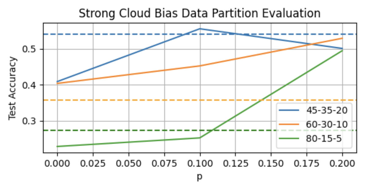
Figure 3: Evaluating the impact of $p$ on the test accuracy for the Cloud Bias (+) training data partition using the “Serving Rate ($p=k$)” strategy. The dashed lines represent the “Equal Weight” strategy’s test accuracy for each serving rate setting. We remind the reader that $p$ stands for the probability that a given client will train each of its smaller exits.

We also analyze two training data partitions that are more extreme, referred to as the strong cloud bias and the strong devices bias cases (see Table 1). In these scenarios, we focus on analyzing the worst-case settings where the expected service rates are higher for the exits having less data points. In particular, we consider serving rates 80-15-5, 60-30-10, and 45-35-20 for the strong cloud bias partition (where the devices store less than 4% of the samples but need to serve a large fraction of requests), and serving rates 5-15-80, 10-30-60, and 20-35-45 for the strong devices bias partition. In the strong cloud bias setting, it can be useful to set $p>0$ for the most powerful clients such that they use their larger datasets to help training the simpler device models. This is an effective way to decrease $\epsilon_{\text{gen}}$, by increasing $|S_{1,\bm{p}}|$ and $|S_{2,\bm{p}}|$, while not having an impact on $\epsilon_{\text{bias}}$. However, there is still a trade-off, because assigning $p>0$ will increase $\epsilon_{\text{opt}}$ due to the later exits training for fewer epochs (as it uses some of its allotted training epochs to train the earlier exits). In Figure 3, we can see that the performance of the “Serving Rate” strategy greatly improves as we increase $p$ progressive from 0 to 0.1 to 0.2. The “Equal Weight” training strategy unsurprisingly struggles in this case because $\epsilon_{\text{gen}}$ for Exit 1 is exceptionally high, due to it having such a small amount of training data, and its static weight assignment has no means of alleviating this issue.

Under the strong devices bias data partition, the system would benefit from weaker clients periodically training the larger exits. Other works such as HeteroFL [3] have considered this scenario assuming that resources limit the size of the model to be used at inference, but not at training. Under this assumption, it would be possible to tune $p$ to obtain exactly the same results as in Figure 3, and in particular the “Serving Rate” strategy would still outperform the “Equal Weight” one. If instead we consider that resource constraints apply both at inference and training, Theorem 1 suggests an alternative approach. The bound indicates that having Exit 3 train on a small dataset may significantly increase $\epsilon_{\text{gen}}$. We can compensate for this effect by selecting $\tilde{\Lambda}_{3}<\Lambda_{3}$ (and conversely $\tilde{\Lambda}_{1}>\Lambda_{1}$) at the expense of introducing a bias $\epsilon_{\text{bias}}>0$. In Table 3, we present the results of a simple heuristic which modifies the aggregation weights in this direction: $\tilde{\Lambda}_{e}=\Lambda_{e}\times\frac{|S_{e,\bm{p}}|}{\text{FLOPS}_{e}}$.

Table 3: Experimental results using the Device Bias (+) data partition for a variety of CIS serving rate settings on the CIFAR10 dataset.

		CIS Serving Rate Setting
Dataset Partition	Strategy	5-15-80	10-30-60	20-35-45
Device Bias (+)	Equal Weight	45.9%	36.7%	29.9%
Device Bias (+)	Serving Rate	44.5%	35.8%	28.8%
Device Bias (+)	Gen. Error Adj	46.2%	35.0%	25.7%

The results show that making this adjustment can be helpful in the extreme worst-case, however it does not outperform either the “Equal Weight” or “Serving Rate” strategies in the other settings.

5 Conclusion and Future Work

We are the first to design an inference-aware FL training algorithm for CISs and we demonstrate that the inference serving rates play a role in all components of the training error. When setting the empirical training weights $\bm{\tilde{\Lambda}}$ equal to the serving rates $\bm{\Lambda}$, our algorithm provides a significant advantage, especially in the case when more requests are served by the devices. However, in certain scenario (e.g., devices have most of the training data while the cloud needs to serve most of the requests), it may be necessary to conceive of more complex rules/heuristics for the choices of $\bm{\tilde{\Lambda}}$ and $\bm{p}$ based on our theoretical bound. We plan to explore these factors in future work. In any case, our rigorous theoretical results are applicable to all hierarchical training systems that rely on assigning importance to each client’s model in the network, including early-exit networks, ordered dropout, pruning, and other nested training methodologies.

This research was supported in part by ANRT in the framework of a CIFRE PhD (2021/0073) and by the Horizon Europe project dAIEDGE.

Appendix A Optimization error

Let us consider the client update rule and the server aggregation rule in our algorithm:

$$\bm{w}_{t,j+1}^{(c,e)} =\bm{w}_{t,j}^{(c,e)}-\eta_{t,j}\frac{1}{\left|\mathcal{B}_{t,j}^{(c,e)}\right|}\sum_{z\in\mathcal{B}_{t,j}^{(c,e)}}\nabla\ell_{e}(\bm{w}_{t,j}^{(c,e)},z),\textrm{ for }j=0,\dots,J-1$$ (17)

$$\bm{w}_{t+1} =\bm{w}_{t}+\eta_{s}\sum_{e\in E}\tilde{\Lambda}_{e}\sum_{c\in N_{t,e}}\frac{|S_{c}|}{S_{e,\bm{p}}}\frac{1}{p_{c,e}}(\bm{w}_{t,J}^{(c,e)}-\bm{w}_{t}),\textrm{ for }t=1,\dots T.$$ (18)

Our proof is similar to the proofs in [30, 29]. We adapt our notation to follow more closely that in those papers. In particular, our proofs are close in spirit to those in [30], but we remove some ambiguities in those proofs (most of the key lemma in that paper are stated under full expectations, but in reality they hold only under proper conditioning). We consider that a client corresponds to the pair $k=(c,e)$, and we define $\alpha_{k}\triangleq\alpha_{c,e}\triangleq\eta_{s}\tilde{\Lambda}_{e}\frac{|S_{c}|}{S_{e,\bm{p}}}$, $\xi_{t}^{k}\triangleq\xi_{t}^{(c,e)}\triangleq\mathbbm{1}_{c\in N_{t,e}}$, and $\nabla F_{k}(\bm{w}_{t,j}^{(c,e)},\mathcal{B}_{\tau}^{k})\triangleq\frac{1}{|\mathcal{B}_{t,j}^{(c,e)}|}\sum_{z\in\mathcal{B}_{t,j}^{(c,e)}}\nabla\ell_{e}(\bm{w}_{t,j}^{(c,e)},z)$.

Moreover, we count gradient steps at clients and aggregation steps at the server using the same time sequence $(\tau=J(t-1)+j)_{t=1,\dots,T,j=0,\dots,J-1}$. The set of values $\mathcal{I}_{J}=\{Jt,t=1,\dots,T\}$ corresponds to the aggregation steps. The equations above can then be rewritten as follows in terms of two new virtual sequences:

$$\bm{v}_{\tau+1}^{k} =\bm{w}_{\tau}^{k}-\eta_{\tau}\nabla F_{k}(\bm{w}_{\tau}^{k},\mathcal{B}_{\tau}^{k})$$ (19)

$$\bm{w}_{\tau+1}^{k} =\begin{dcases*}\bm{w}_{1}&for $\tau+1=0$,\\ \Pi_{W}\left(\bm{w}_{\tau+1-J}^{k}+\sum_{k\in\mathcal{K}}\frac{\alpha_{k}\xi_{\tau+1-J}^{k}}{p_{k}}(\bm{v}_{\tau+1}^{k}-\bm{w}_{\tau+1-J}^{k})\right)&for $\tau+1\in\mathcal{I}_{J}$,\\ \bm{v}_{\tau+1}^{k}&otherwise.\\ \end{dcases*}$$ (20)

$\bm{v}_{J(t-1)+j}^{k}$ coincides then with the local model $\bm{w}_{t,j}^{(c,e)}$ and $\bm{w}^{k}_{J(t-1)}$ coincides with the global model $\bm{w}_{t}$.

We observe that, for $\tau+1\in\mathcal{I}_{J}$, $\bm{w}_{\tau+1}^{k}=\bm{w}_{\tau+1}^{k^{\prime}}$ for any $k$ and $k^{\prime}$, and that, for $\tau+1\not\in\mathcal{I}_{J}$, ${\bm{v}}_{\tau+1}^{k}={\bm{w}}_{\tau+1}^{k}$. Moreover, define the average sequences $\bar{\bm{v}}_{\tau+1}=\sum_{k\in\mathcal{K}}\alpha_{k}\bm{v}_{\tau+1}^{k}$ and $\bar{\bm{w}}_{\tau+1}=\sum_{k\in\mathcal{K}}\alpha_{k}\bm{w}_{\tau+1}^{k}$ and similarly the average gradients $\bm{g}_{\tau}=\sum_{k\in\mathcal{K}}\alpha_{k}\nabla F_{k}(\bm{w}_{\tau}^{k},\mathcal{B}_{t}^{k})$ and $\bar{\bm{g}}_{\tau}=\sum_{k\in\mathcal{K}}\alpha_{k}\nabla F_{k}(\bm{w}_{\tau}^{k})$. We also define the sequence

$$\bar{\bm{w}}_{\tau+1}^{\dagger}=\begin{dcases*}\bm{w}_{\tau+1-J}^{k}+\sum_{k\in\mathcal{K}}\frac{\alpha_{k}\xi_{\tau+1-J}^{k}}{p_{k}}(\bm{v}_{\tau+1}^{k}-\bm{w}_{\tau+1-J}^{k}),&for $\tau+1\in\mathcal{I}_{J}$\\ \bar{\bm{w}}_{\tau+1},&otherwise.\end{dcases*}$$ (21)

We note that $\bar{\bm{w}}_{\tau+1}=\Pi_{W}\left(\bar{\bm{w}}_{\tau+1}^{\dagger}\right)$ for $\tau+1\in\mathcal{I}_{J}$ and coincide otherwise.

We denote by $\mathcal{B}_{\tau}=(\mathcal{B}_{\tau}^{k})_{k\in\mathcal{K}}$ and $\xi_{\tau}=(\xi_{\tau}^{k})_{k\in\mathcal{K}}$, the set of batches and the set of indicator variables for client participation at instant $\tau$. The history of the system at time $\tau$ is made by the values of the random variables until that time and it can be defined by recursion as follows: $\mathcal{H}_{1}=\emptyset$, $\mathcal{H}_{\tau+1}=\{\xi_{\tau+1},\mathcal{B}_{\tau},\mathcal{H}_{\tau}\}$ if $\tau+1\in\mathcal{I}_{J}$ and $\mathcal{H}_{\tau+1}=\{\mathcal{B}_{\tau},\mathcal{H}_{\tau}\}$, otherwise.

We define $G_{c,e}\triangleq\sigma^{2}_{c,e}+(L\operatorname{diam}(W))^{2}$ and observe that it bounds the second moment of the stochastic gradient at $(c,e)$:

$$\mathbb{E}\left[\left\lVert\nabla F_{c,e}(\bm{w},\mathcal{B})\right\rVert^{2}\right] =\mathbb{E}\left[\left\lVert\nabla F_{c,e}(\bm{w},\mathcal{B})-\nabla F_{c,e}(\bm{w})\right\rVert^{2}\right]+\left\lVert\nabla F_{c,e}(\bm{w})\right\rVert^{2}$$ (22)

$$\leq\sigma_{c,e}^{2}+L^{2}\left\lVert\bm{w}-\bm{w}_{c,e}^{*}\right\rVert^{2}$$ (23)

$$\leq\sigma_{c,e}^{2}+L^{2}\operatorname{diam}(W)^{2}=G_{c,e},$$ (24)

where we have used Assumption 2. We also define a uniform bound over all clients and all exits: $G\triangleq\max_{(c,e)\in\mathcal{K}}G_{c,e}$.

Similarly to other works [15, 13, 37, 38], we introduce a metric to quantify the heterogeneity of clients’ local datasets, typically referred to as statistical heterogeneity:

$$\Gamma \triangleq\max_{(c,e)\in\mathcal{K}}F_{c,e}(\bm{w}_{\bm{\tilde{\Lambda}}}^{\star})-F_{c,e}^{\star}.$$ (25)

Finally, we define $h(\tau)\triangleq\max\{\tau^{\prime}\in\mathcal{I}_{J}:\tau^{\prime}\leq\tau\}$. Then $h(\tau)$ indicates the time of the last server update before $\tau$.

The following lemma corresponds to [30, Lemma 4].

Lemma 1.

$$\mathbb{E}_{\mathcal{B}_{\tau},\dots,\mathcal{B}_{h(\tau)}\mid\mathcal{H}_{h(\tau)}}\left\lVert\bar{\bm{v}}_{\tau+1}-\bm{w}^{\star}_{\bm{\tilde{\Lambda}}}\right\rVert \leq(1-\eta_{\tau}\mu)\mathbb{E}_{\mathcal{B}_{\tau-1},\dots,\mathcal{B}_{h(\tau)}\mid\mathcal{H}_{h(\tau)}}\left\lVert\bar{\bm{w}}_{\tau}-\bm{w}^{\star}_{\bm{\tilde{\Lambda}}}\right\rVert+\eta_{\tau}^{2}\left(\sum_{k\in\mathcal{K}}\alpha_{k}^{2}\sigma_{k}^{2}+6L\Gamma+8(J-1)^{2}G^{2}\right).$$ (26)

Proof.

From [16, Lemma 1]:

$$\mathbb{E}_{\mathcal{B}_{\tau}\mid\mathcal{H}_{\tau}}\left\lVert\bar{\bm{v}}_{\tau+1}-\bm{w}^{\star}_{\bm{\tilde{\Lambda}}}\right\rVert \leq(1-\eta_{\tau}\mu)\left\lVert\bar{\bm{w}}_{\tau}-\bm{w}^{\star}_{\bm{\tilde{\Lambda}}}\right\rVert+\eta_{\tau}^{2}\mathbb{E}_{\mathcal{B}_{\tau}\mid\mathcal{H}_{\tau}}\left\lVert\bm{g}_{\tau}-\bar{\bm{g}}_{\tau}\right\rVert^{2}+\eta_{\tau}^{2}6L\Gamma+2\sum_{k\in\mathcal{K}}\alpha_{k}\left\lVert\bm{w}_{\tau}^{k}-\bar{\bm{w}}_{\tau}\right\rVert^{2}.$$ (27)

From [16, Lemma 2]:

$$\mathbb{E}_{\mathcal{B}_{\tau}\mid\mathcal{H}_{\tau}}\left\lVert\bm{g}_{\tau}-\bar{\bm{g}}_{\tau}\right\rVert^{2} \leq\mathbb{E}_{\mathcal{B}_{\tau}\mid\mathcal{H}_{\tau}}\left\lVert\sum_{k\in\mathcal{K}}\alpha_{k}\left(\nabla F_{k}(\bm{w}_{t}^{k},\mathcal{B}_{\tau}^{k})-\nabla F_{k}(\bm{w}_{t}^{k})\right)\right\rVert^{2}$$ (28)

$$=\sum_{k\in\mathcal{K}}\alpha_{k}^{2}\mathbb{E}_{\mathcal{B}_{\tau}^{k}\mid\mathcal{H}_{t}}\left\lVert\nabla F_{k}(\bm{w}_{t}^{k},\mathcal{B}_{\tau}^{k})-\nabla F_{k}(\bm{w}_{t}^{k})\right\rVert^{2}$$ (29)

$$\leq\sum_{k\in\mathcal{K}}\alpha_{k}^{2}\sigma_{k}^{2}.$$ (30)

Combining the two inequalities above:

$$\mathbb{E}_{\mathcal{B}_{\tau}\mid\mathcal{H}_{\tau}}\left\lVert\bar{\bm{v}}_{\tau+1}-\bm{w}^{\star}_{\bm{\tilde{\Lambda}}}\right\rVert \leq(1-\eta_{\tau}\mu)\left\lVert\bar{\bm{w}}_{\tau}-\bm{w}^{\star}_{\bm{\tilde{\Lambda}}}\right\rVert+\eta_{\tau}^{2}\sum_{k\in\mathcal{K}}\alpha_{k}^{2}\sigma_{k}^{2}+\eta_{\tau}^{2}6L\Gamma+2\sum_{k\in\mathcal{K}}\alpha_{k}\left\lVert\bm{w}_{\tau}^{k}-\bar{\bm{w}}_{\tau}\right\rVert^{2}.$$ (31)

Define $h(\tau)\triangleq\max\{\tau^{\prime}\in\mathcal{I}_{J}:\tau^{\prime}\leq\tau\}$. We observe that $0\leq\tau-h(\tau)\leq J-1$ and $\mathcal{H}_{\tau}=\{\mathcal{B}_{\tau-1},B_{\tau-2},\dots,B_{h(\tau)},\mathcal{H}_{h(\tau)}\}$. From [16, Lemma 3]:

$$\sum_{k\in\mathcal{K}}\alpha_{k}\mathbb{E}_{\mathcal{B}_{\tau-1},\dots,\mathcal{B}_{h(\tau)}\mid\mathcal{H}_{h(\tau)}}\left\lVert\bm{w}_{\tau}^{k}-\bar{\bm{w}}_{\tau}\right\rVert^{2} =\sum_{k\in\mathcal{K}}\alpha_{k}\mathbb{E}_{\mathcal{B}_{\tau-1},\dots,\mathcal{B}_{h(\tau)}\mid\mathcal{H}_{h(\tau)}}\left\lVert(\bm{w}_{\tau}^{k}-\bar{\bm{w}}_{h(\tau)})-(\bar{\bm{w}}_{\tau}-\bar{\bm{w}}_{h(\tau)})\right\rVert^{2}$$ (32)

$$\leq\sum_{k\in\mathcal{K}}\alpha_{k}\mathbb{E}_{\mathcal{B}_{\tau-1},\dots,\mathcal{B}_{h(\tau)}\mid\mathcal{H}_{h(\tau)}}\left\lVert\bm{w}_{\tau}^{k}-\bar{\bm{w}}_{h(\tau)}\right\rVert^{2}$$ (33)

$$=\sum_{k\in\mathcal{K}}\alpha_{k}\mathbb{E}_{\mathcal{B}_{\tau-1},\dots,\mathcal{B}_{h(\tau)}\mid\mathcal{H}_{h(\tau)}}\left\lVert\sum_{i=h(\tau)}^{t-1}\eta_{i}\nabla F_{k}(\bm{w}_{i}^{k},\mathcal{B}_{i}^{k})\right\rVert^{2}$$ (34)

$$\leq\sum_{k\in\mathcal{K}}\alpha_{k}(\tau-h(\tau))\mathbb{E}_{\mathcal{B}_{\tau-1},\dots,\mathcal{B}_{h(\tau)}\mid\mathcal{H}_{h(\tau)}}\left[\sum_{i=h(\tau)}^{t-1}\eta_{i}^{2}\left\lVert\nabla F_{k}(\bm{w}_{i}^{k},\mathcal{B}_{i}^{k})\right\rVert^{2}\right]$$ (35)

$$\leq\eta_{h(\tau)}^{2}(t-h(\tau))^{2}G^{2}\leq 4\eta_{\tau}^{2}(J-1)^{2}G^{2}.\vphantom{\sum_{k\in\mathcal{K}}}$$ (36)

By repeatedly computing expectations over the previous batch conditioned on the previous history and combining the inequalities above, we obtain:

$$\mathbb{E}_{\mathcal{B}_{\tau},\dots,\mathcal{B}_{h(\tau)}\mid\mathcal{H}_{h(\tau)}}\left\lVert\bar{\bm{v}}_{\tau+1}-\bm{w}^{\star}_{\bm{\tilde{\Lambda}}}\right\rVert \leq(1-\eta_{\tau}\mu)\mathbb{E}_{\mathcal{B}_{\tau-1},\dots,\mathcal{B}_{h(\tau)}\mid\mathcal{H}_{h(\tau)}}\left\lVert\bar{\bm{w}}_{\tau}-\bm{w}^{\star}_{\bm{\tilde{\Lambda}}}\right\rVert+\eta_{\tau}^{2}\left(\sum_{k\in\mathcal{K}}\alpha_{k}^{2}\sigma_{k}^{2}+6L\Gamma+8(J-1)^{2}G^{2}\right).$$ (37)

∎

The following lemma corresponds to [30, Lemma 2], but it needs to be adapted to take into account the projection.

Lemma 2.

$$\mathbb{E}_{\xi_{h(\tau)}\mid\mathcal{B}_{\tau},\dots,\mathcal{B}_{h(\tau)+1},\mathcal{H}_{h(\tau)}}[\bar{\bm{w}}_{\tau+1}^{\dagger}]=\bar{\bm{v}}_{\tau+1}.$$ (38)

Proof.

First, we observe that $\bar{\bm{w}}^{\dagger}_{\tau+1}=\bar{\bm{w}}_{\tau+1}=\bar{\bm{v}}_{\tau+1}$ for $\tau+1\not\in\mathcal{I}_{J}$. For $\tau+1\in\mathcal{I}_{J}$, $h(\tau)=\tau+1-J$ and

$$\mathbb{E}_{\xi_{\tau+1-J}\mid\mathcal{B}_{\tau},\dots,\mathcal{B}_{\tau+1-J},\mathcal{H}_{\tau+1-J}}[\bar{\bm{w}}_{\tau+1}^{\dagger}] =\bar{\bm{w}}_{\tau+1-J}-\sum_{k\in\mathcal{K}}\frac{\alpha_{k}\mathbb{E}[\xi_{\tau+1-J}^{k}]}{p_{k}}\sum_{j=0}^{J-1}\eta_{\tau+1-J+j}\nabla F_{k}(\bm{w}_{\tau+1-J+j}^{k},\mathcal{B}_{\tau+1-J+j}^{k})$$ (39)

$$=\bar{\bm{w}}_{\tau+1-J}-\sum_{k\in\mathcal{K}}\alpha_{k}\sum_{j=0}^{J-1}\eta_{\tau+1-J+j}\nabla F_{k}(\bm{w}_{\tau+1-J+j}^{k},\mathcal{B}_{\tau+1-J+j}^{k})=\bar{\bm{v}}_{\tau+1}.$$ (40)

∎

The following lemma corresponds to [30, Lemma 3]. We modify the proof to take into account the correlation in the participation of the fictitious clients in $\mathcal{K}$. Indeed, each client $c$ selects a single exit to train and then the random variables $\{\xi_{h(\tau)}\}_{e\in E}$ are (negatively) correlated.

Lemma 3.

$$\mathbb{E}_{\mathcal{B}_{\tau},\dots,\mathcal{B}_{h(\tau)},\xi_{h(\tau)}\mid\mathcal{H}_{h(\tau)}}\left\lVert\bar{\bm{w}}_{\tau+1}^{\dagger}-\bar{\bm{v}}_{\tau+1}\right\rVert^{2} \leq 4\eta_{\tau}^{2}J^{2}G^{2}\sum_{c=1}^{N}\left(\sum_{e\in E_{c}}\frac{\alpha_{c,e}^{2}}{p_{c,e}}-\left(\sum_{e\in E_{c}}\alpha_{c,e}\right)^{2}\right).$$ (41)

Proof.

We have a tighter bound ($\alpha_{k}^{2}$ instead of $\alpha_{k}$), observing that $\operatorname{Var}(X)=\mathbb{E}[X-\mathbb{E}[X]]^{2}$. Let $\bm{X}$ be a d-dimensional random variable, we define its variance as follows: $\operatorname{{\mathbb{V}ar}}(\bm{X})\triangleq\sum_{i=1}^{d}\operatorname{Var}(X_{i})$. We also denote by $E_{c}$ the set of exits client $c$ may train, i.e., $E_{c}\triangleq\{e:p_{c,e}>0,e=1,\dots,E\}$.

In order to keep the following calculations simpler to follow, we denote by $\bm{U}_{c,e}=\sum_{j=0}^{\tau-h(\tau)}\eta_{h(\tau)+j}\nabla F_{c,e}(\bm{w}_{h(\tau)+j}^{(c,e)},\mathcal{B}_{h(\tau)+j}^{(c,e)})$.

$$\mathbb{E}_{\xi_{h(\tau)}\mid\mathcal{B}_{\tau},\dots,\mathcal{B}_{h(\tau)},\mathcal{H}_{h(\tau)}} \left\lVert\bar{\bm{w}}_{\tau+1}^{\dagger}-\bar{\bm{v}}_{\tau+1}\right\rVert^{2}$$

$$=\operatorname{{\mathbb{V}ar}}_{\xi_{h(\tau)}\mid\mathcal{B}_{\tau},\dots,\mathcal{B}_{h(\tau)},\mathcal{H}_{h(\tau)}}\left(\sum_{k\in\mathcal{K}}\frac{\alpha_{k}\xi_{h(\tau)}^{k}}{p_{k}}\sum_{j=0}^{\tau-h(\tau)}\eta_{h(\tau)+j}\nabla F_{k}(\bm{w}_{h(\tau)+j}^{k},\mathcal{B}_{h(\tau)+j}^{k})\right)$$ (42)

$$=\operatorname{{\mathbb{V}ar}}_{\xi_{h(\tau)}\mid\mathcal{B}_{\tau},\dots,\mathcal{B}_{h(\tau)},\mathcal{H}_{h(\tau)}}\left(\sum_{c=1}^{N}\sum_{e\in E_{c}}\frac{\alpha_{c,e}\xi_{h(\tau)}^{(c,e)}}{p_{c,e}}\bm{U}_{c,e}\right)$$ (43)

$$=\sum_{c=1}^{N}\operatorname{{\mathbb{V}ar}}_{\xi_{h(\tau)}\mid\mathcal{B}_{\tau},\dots,\mathcal{B}_{h(\tau)},\mathcal{H}_{h(\tau)}}\left(\sum_{e\in E_{c}}\frac{\alpha_{c,e}\xi_{h(\tau)}^{(c,e)}}{p_{c,e}}\bm{U}_{c,e}\right)$$ (44)

$$\leq\sum_{c=1}^{N}\sum_{e\in E_{c}}\operatorname{{\mathbb{V}ar}}_{\xi_{h(\tau)}\mid\mathcal{B}_{\tau},\dots,\mathcal{B}_{h(\tau)},\mathcal{H}_{h(\tau)}}\left(\frac{\alpha_{c,e}\xi_{h(\tau)}^{(c,e)}}{p_{c,e}}\bm{U}_{c,e}\right)$$ (45)

$$=\sum_{c=1}^{N}\sum_{e\in E_{c}}\operatorname{Var}\left(\frac{\alpha_{c,e}\xi_{h(\tau)}^{(c,e)}}{p_{c,e}}\right)\left\lVert\bm{U}_{c,e}\right\rVert^{2}$$ (46)

$$=\sum_{c=1}^{N}\sum_{e\in E_{c}}\alpha_{c,e}^{2}\frac{1-p_{c,e}}{p_{c,e}}\left\lVert\bm{U}_{c,e}\right\rVert^{2}.$$ (47)

where (45) takes into account that $\xi_{\tau+1-J}^{(c,e)}\xi_{\tau+1-J}^{(c,e^{\prime})}=0$ for $e\neq e^{\prime}$ because each client selects a single exit to train.

Then, the expectation over the random batches is computed

$$\mathbb{E}_{\mathcal{B}_{\tau},\dots,\mathcal{B}_{h(\tau)},\xi_{h(\tau)}\mid\mathcal{H}_{h(\tau)}} \left\lVert\bar{\bm{w}}_{\tau+1}^{\dagger}-\bar{\bm{v}}_{\tau+1}\right\rVert^{2}$$

$$\leq\sum_{c=1}^{N}\sum_{e\in E_{c}}\alpha_{c,e}^{2}\frac{1-p_{c,e}}{p_{c,e}}\mathbb{E}_{\mathcal{B}_{\tau},\dots,\mathcal{B}_{h(\tau)}\mid\mathcal{H}_{h(\tau)}}\left[\left\lVert\bm{U}_{c,e}\right\rVert^{2}\right]$$ (48)

$$\leq\sum_{c=1}^{N}\sum_{e\in E_{c}}\alpha_{c,e}^{2}\frac{1-p_{c,e}}{p_{c,e}}\mathbb{E}_{\mathcal{B}_{\tau},\dots,\mathcal{B}_{h(\tau)}\mid\mathcal{H}_{h(\tau)}}\left[\left\lVert\sum_{j=0}^{\tau-h(\tau)}\eta_{h(\tau)+j}\nabla F_{c,e}(\bm{w}_{h(\tau)+j}^{(c,e)},\mathcal{B}_{h(\tau)+j}^{(c,e)})\right\rVert^{2}\right]$$ (49)

$$\leq\eta_{h(\tau)+j}^{2}J\sum_{c=1}^{N}\sum_{e\in E_{c}}\alpha_{c,e}^{2}\frac{1-p_{c,e}}{p_{c,e}}\sum_{j=0}^{\tau-h(\tau)}\mathbb{E}_{\mathcal{B}_{\tau},\dots,\mathcal{B}_{h(\tau)}\mid\mathcal{H}_{h(\tau)}}\left[\left\lVert\nabla F_{c,e}(\bm{w}_{h(\tau)+j}^{(c,e)},\mathcal{B}_{h(\tau)+j}^{(c,e)})\right\rVert^{2}\right]$$ (50)

$$\leq\eta_{h(\tau)+j}^{2}J^{2}\sum_{c=1}^{N}\sum_{e\in E_{c}}\alpha_{c,e}^{2}\frac{1-p_{c,e}}{p_{c,e}}G_{c,e}$$ (51)

$$\leq 4\eta_{\tau}^{2}J^{2}\sum_{c=1}^{N}\sum_{e\in E_{c}}\alpha_{c,e}^{2}\frac{1-p_{c,e}}{p_{c,e}}G_{c,e},$$ (52)

where (52) uses $\eta_{h(\tau)+j}\leq\eta_{\tau-J}\leq 2\eta_{\tau}$. ∎

Theorem 2.

Under Assumptions 2–5, the optimization error of Algorithm 1 with learning rate $\eta_{t,j}=\frac{2}{\mu(\gamma+(t-1)J+j+1)}$ and $\gamma\triangleq\max\{8\kappa,J\}-1$ can be bounded as follows:

$$\mathbb{E}\left[F_{S,\bm{\tilde{\Lambda}}}(\bm{w}_{T})\right]-F_{S,\bm{\tilde{\Lambda}}}^{\star}=\frac{\kappa}{\gamma+JT}\left(\frac{2B}{\mu}+\frac{\mu(\gamma+1)}{2}\mathbb{E}\left[\bm{w}_{1}-\bm{w}^{\star}_{\bm{\tilde{\Lambda}}}\right]\right),$$ (53)

where

$$B\triangleq\sum_{(c,e)\in\mathcal{K}}\alpha_{c,e}^{2}\sigma_{c,e}^{2}+6L\Gamma+8(J-1)^{2}G^{2}+4J^{2}\sum_{c=1}^{N}\sum_{e\in E_{c}}\alpha_{c,e}^{2}\frac{1-p_{c,e}}{p_{c,e}}G_{c,e},$$ (54)

$$G_{c,e}\triangleq\sigma^{2}_{c,e}+(L\operatorname{diam}(W))^{2},$$ (55)

$$G\triangleq\max_{(c,e)\in\mathcal{K}}G_{c,e},$$ (56)

$$\alpha_{c,e}\triangleq\eta_{s}\tilde{\Lambda}_{e}\frac{|S_{c}|}{S_{e,\bm{p}}}.$$ (57)

Proof.

As we mention at the beginning of this appendix, we count gradient steps at clients and aggregation steps at the server using the same time sequence $(\tau=J(t-1)+j)_{t=1,\dots,T,j=0,\dots,J-1}$. The set of values $\mathcal{I}_{J}=\{Jt,t=1,\dots,T\}$ corresponds to the aggregation steps.

We have

$$\left\lVert\bar{\bm{w}}_{\tau+1}-\bm{w}^{\star}_{\bm{\tilde{\Lambda}}}\right\rVert^{2} \leq\left\lVert\bar{\bm{w}}_{\tau+1}^{\dagger}-\bm{w}^{\star}_{\bm{\tilde{\Lambda}}}\right\rVert^{2}$$ (58)

$$=\left\lVert\bar{\bm{w}}_{\tau+1}^{\dagger}-\bar{\bm{v}}_{\tau+1}+\bar{\bm{v}}_{\tau+1}-\bm{w}^{\star}_{\bm{\tilde{\Lambda}}}\right\rVert^{2}$$ (59)

$$=\left\lVert\bar{\bm{w}}_{\tau+1}^{\dagger}-\bar{\bm{v}}_{\tau+1}\right\rVert^{2}+\left\lVert\bar{\bm{v}}_{\tau+1}-\bm{w}^{\star}_{\bm{\tilde{\Lambda}}}\right\rVert^{2}+2\langle\bar{\bm{w}}_{\tau+1}^{\dagger}-\bar{\bm{v}}_{\tau+1},\bar{\bm{v}}_{\tau+1}-\bm{w}^{\star}_{\bm{\tilde{\Lambda}}}\rangle,$$ (60)

where the first inequality is trivially true for $\tau+1\not\in\mathcal{I}_{J}$ because $\bar{\bm{w}}_{\tau+1}=\bar{\bm{w}}_{\tau+1}^{\dagger}$, while for $\tau+1\not\in\mathcal{I}_{J}$, it follows from Assumption 2 and$\left\lVert\bar{\bm{w}}_{\tau+1}-\bm{w}^{\star}_{\bm{\tilde{\Lambda}}}\right\rVert^{2}=\left\lVert\Pi_{W}(\bar{\bm{w}}_{\tau+1}^{\dagger})-\Pi_{W}(\bm{w}^{\star}_{\bm{\tilde{\Lambda}}})\right\rVert^{2}\leq\left\lVert\bar{\bm{w}}_{\tau+1}^{\dagger}-\bm{w}^{\star}_{\bm{\tilde{\Lambda}}}\right\rVert^{2}$.

We take expectation over clients’ participation

$$\mathbb{E}_{\xi_{h(\tau)}\mid\mathcal{B}_{\tau},\dots,\mathcal{B}_{h(\tau)},\mathcal{H}_{h(\tau)}}\left\lVert\bar{\bm{w}}_{\tau+1}-\bm{w}^{\star}_{\bm{\tilde{\Lambda}}}\right\rVert^{2} \leq\left\lVert\bar{\bm{v}}_{\tau+1}-\bm{w}^{\star}_{\bm{\tilde{\Lambda}}}\right\rVert^{2}+\mathbb{E}_{\xi_{h(\tau)}\mid\mathcal{B}_{\tau},\dots,\mathcal{B}_{h(\tau)},\mathcal{H}_{h(\tau)}}\left\lVert\bar{\bm{w}}_{\tau+1}^{\dagger}-\bar{\bm{v}}_{\tau+1}\right\rVert^{2}$$ (61)

$$\leq\left\lVert\bar{\bm{v}}_{\tau+1}-\bm{w}^{\star}_{\bm{\tilde{\Lambda}}}\right\rVert^{2}+4\eta_{\tau}^{2}J^{2}\sum_{c=1}^{N}\sum_{e\in E_{c}}\alpha_{c,e}^{2}\frac{1-p_{c,e}}{p_{c,e}}G_{c,e},$$ (62)

where the equality derives from Lemma 2 and the inequality from Lemma 3. We take then expectation over the random batches

$$\mathbb{E}_{\mathcal{B}_{\tau},\dots,\mathcal{B}_{h(\tau)},\xi_{h(\tau)}\mid\mathcal{H}_{h(\tau)}} \left\lVert\bar{\bm{w}}_{\tau+1}-\bm{w}^{\star}_{\bm{\tilde{\Lambda}}}\right\rVert^{2}$$

$$\leq\mathbb{E}_{\mathcal{B}_{\tau},\dots,\mathcal{B}_{h(\tau)}\mid\mathcal{H}_{h(\tau)}}\left\lVert\bar{\bm{v}}_{\tau+1}-\bm{w}^{\star}_{\bm{\tilde{\Lambda}}}\right\rVert^{2}+4\eta_{\tau}^{2}J^{2}\sum_{c=1}^{N}\sum_{e\in E_{c}}\alpha_{c,e}^{2}\frac{1-p_{c,e}}{p_{c,e}}G_{c,e}$$ (63)

$$\leq(1-\eta_{\tau}\mu)\mathbb{E}_{\mathcal{B}_{\tau-1},\dots,\mathcal{B}_{h(\tau)}\mid\mathcal{H}_{h(\tau)}}\left\lVert\bar{\bm{w}}_{\tau}-\bm{w}^{\star}_{\bm{\tilde{\Lambda}}}\right\rVert+\eta_{\tau}^{2}\left(\sum_{k\in\mathcal{K}}\alpha_{k}^{2}\sigma_{k}^{2}+6L\Gamma+8(J-1)^{2}G^{2}\right)$$

$$+4\eta_{\tau}^{2}J^{2}\sum_{c=1}^{N}\sum_{e\in E_{c}}\alpha_{c,e}^{2}\frac{1-p_{c,e}}{p_{c,e}}G_{c,e},$$ (64)

where the last inequality follows from Lemma 1 observing that if $\tau+1\in\mathcal{I}_{J}$, then $h(\tau)=\tau+1-J$.

Finally, we take total expectation

$$\mathbb{E}\left\lVert\bar{\bm{w}}_{\tau+1}-\bm{w}^{\star}_{\bm{\tilde{\Lambda}}}\right\rVert^{2}\leq(1-\eta_{\tau}\mu)\mathbb{E}\left\lVert\bar{\bm{w}}_{\tau}-\bm{w}^{\star}_{\bm{\tilde{\Lambda}}}\right\rVert+\eta_{\tau}^{2}\left(\sum_{k\in\mathcal{K}}\alpha_{k}^{2}\sigma_{k}^{2}+6L\Gamma+8(J-1)^{2}G^{2}+4J^{2}\sum_{c=1}^{N}\sum_{e\in E_{c}}\alpha_{c,e}^{2}\frac{1-p_{c,e}}{p_{c,e}}G_{c,e}\right).$$ (65)

This leads to a recurrence relation of the form $\Delta_{\tau+1}\leq(1-\eta_{\tau}\mu)\Delta_{\tau}+\eta_{\tau}^{2}B,$ and the result is obtained following the same steps in the proof of [16, Thm. 1]. ∎

References

- Baccarelli et al. [2020] E. Baccarelli, S. Scardapane, M. Scarpiniti, A. Momenzadeh, and A. Uncini. Optimized training and scalable implementation of conditional deep neural networks with early exits for fog-supported iot applications. Inf. Sci., 521:107–143, 2020. 10.1016/j.ins.2020.02.041. URL https://doi.org/10.1016/j.ins.2020.02.041.
- Bousquet et al. [2003] O. Bousquet, S. Boucheron, and G. Lugosi. Introduction to statistical learning theory. In O. Bousquet, U. von Luxburg, and G. Rätsch, editors, Advanced Lectures on Machine Learning, volume 3176 of Lecture Notes in Computer Science, pages 169–207. Springer, 2003. ISBN 3-540-23122-6.
- Diao et al. [2020] E. Diao, J. Ding, and V. Tarokh. Heterofl: Computation and communication efficient federated learning for heterogeneous clients. arXiv preprint arXiv:2010.01264, 2020.
- He et al. [2016] K. He, X. Zhang, S. Ren, and J. Sun. Deep residual learning for image recognition. In Proceedings of the IEEE conference on computer vision and pattern recognition, pages 770–778, 2016.
- Horvath et al. [2021] S. Horvath, S. Laskaridis, M. Almeida, I. Leontiadis, S. Venieris, and N. Lane. Fjord: Fair and accurate federated learning under heterogeneous targets with ordered dropout. Advances in Neural Information Processing Systems, 34:12876–12889, 2021.
- Hu et al. [2019] H. Hu, D. Dey, M. Hebert, and J. A. Bagnell. Learning anytime predictions in neural networks via adaptive loss balancing. In The Thirty-Third AAAI Conference on Artificial Intelligence, AAAI 2019, pages 3812–3821. AAAI Press, 2019. 10.1609/aaai.v33i01.33013812. URL https://doi.org/10.1609/aaai.v33i01.33013812.
- Huang et al. [2018] G. Huang, D. Chen, T. Li, F. Wu, L. van der Maaten, and K. Q. Weinberger. Multi-scale dense networks for resource efficient image classification. In 6th International Conference on Learning Representations, ICLR 2018, Vancouver, BC, Canada, April 30 - May 3, 2018, Conference Track Proceedings. OpenReview.net, 2018. URL https://openreview.net/forum?id=Hk2aImxAb.
- Ilhan et al. [2023] F. Ilhan, G. Su, and L. Liu. Scalefl: Resource-adaptive federated learning with heterogeneous clients. In Proceedings of the IEEE/CVF Conference on Computer Vision and Pattern Recognition, pages 24532–24541, 2023.
- Kairouz et al. [2021] P. Kairouz, H. B. McMahan, B. Avent, A. Bellet, M. Bennis, A. N. Bhagoji, K. Bonawitz, Z. Charles, G. Cormode, R. Cummings, et al. Advances and open problems in federated learning. Foundations and trends® in machine learning, 14(1–2):1–210, 2021.
- Kaya et al. [2019] Y. Kaya, S. Hong, and T. Dumitras. Shallow-deep networks: Understanding and mitigating network overthinking. In International conference on machine learning, pages 3301–3310. PMLR, 2019.
- Li et al. [2019a] E. Li, L. Zeng, Z. Zhou, and X. Chen. Edge ai: On-demand accelerating deep neural network inference via edge computing. IEEE Transactions on Wireless Communications, 19(1):447–457, 2019a.
- Li et al. [2019b] H. Li, H. Zhang, X. Qi, R. Yang, and G. Huang. Improved techniques for training adaptive deep networks. In Proceedings of the IEEE/CVF International Conference on Computer Vision, pages 1891–1900, 2019b.
- Li et al. [2020a] T. Li, A. K. Sahu, A. Talwalkar, and V. Smith. Federated learning: Challenges, methods, and future directions. IEEE signal processing magazine, 37(3):50–60, 2020a.
- Li et al. [2020b] T. Li, A. K. Sahu, M. Zaheer, M. Sanjabi, A. Talwalkar, and V. Smith. Federated optimization in heterogeneous networks. Proceedings of Machine learning and systems, 2:429–450, 2020b.
- Li et al. [2019c] X. Li, K. Huang, W. Yang, S. Wang, and Z. Zhang. On the Convergence of FedAvg on Non-IID Data. In International Conference on Learning Representations, 2019c.
- Li et al. [2020c] X. Li, K. Huang, W. Yang, S. Wang, and Z. Zhang. On the Convergence of FedAvg on Non-IID Data. In International Conference on Learning Representations, Apr. 2020c.
- Lim et al. [2020] W. Y. B. Lim, N. C. Luong, D. T. Hoang, Y. Jiao, Y.-C. Liang, Q. Yang, D. Niyato, and C. Miao. Federated learning in mobile edge networks: A comprehensive survey. IEEE Communications Surveys & Tutorials, 22(3):2031–2063, 2020.
- Lin et al. [2020] T. Lin, L. Kong, S. U. Stich, and M. Jaggi. Ensemble distillation for robust model fusion in federated learning. Advances in Neural Information Processing Systems, 33:2351–2363, 2020.
- [19] M. Livesay. Chaining method to improve rademacher bound. URL https://courses.engr.illinois.edu/ece543/sp2017/projects/projects.html.
- Malka et al. [2022] M. Malka, E. Farhan, H. Morgenstern, and N. Shlezinger. Decentralized low-latency collaborative inference via ensembles on the edge. arXiv preprint arXiv:2206.03165, 2022.
- Marfoq et al. [2023] O. Marfoq, G. Neglia, L. Kameni, and R. Vidal. Federated learning for data streams. In F. Ruiz, J. Dy, and J.-W. van de Meent, editors, Proceedings of The 26th International Conference on Artificial Intelligence and Statistics, volume 206 of Proceedings of Machine Learning Research, pages 8889–8924. PMLR, 25–27 Apr 2023. URL https://proceedings.mlr.press/v206/marfoq23a.html.
- Matsubara et al. [2022] Y. Matsubara, M. Levorato, and F. Restuccia. Split computing and early exiting for deep learning applications: Survey and research challenges. ACM Computing Surveys, 55(5):1–30, 2022.
- McMahan et al. [2017] B. McMahan, E. Moore, D. Ramage, S. Hampson, and B. A. y Arcas. Communication-efficient learning of deep networks from decentralized data. In Artificial intelligence and statistics, pages 1273–1282. PMLR, 2017.
- Mohri et al. [2018] M. Mohri, A. Rostamizadeh, and A. Talwalkar. Foundations of Machine Learning. Adaptive Computation and Machine Learning. MIT Press, Cambridge, MA, 2 edition, 2018. ISBN 978-0-262-03940-6.
- Mora et al. [2022] A. Mora, I. Tenison, P. Bellavista, and I. Rish. Knowledge distillation for federated learning: a practical guide. arXiv preprint arXiv:2211.04742, 2022.
- Nawar et al. [2023] M. N. A. M. Nawar, D. Falavigna, and A. Brutti. Fed-ee: Federating heterogeneous asr models using early-exit architectures. In Proceedings of 3rd Neurips Workshop on Efficient Natural Language and Speech Processing, 2023.
- Ren et al. [2023] W.-Q. Ren, Y.-B. Qu, C. Dong, Y.-Q. Jing, H. Sun, Q.-H. Wu, and S. Guo. A survey on collaborative dnn inference for edge intelligence. Machine Intelligence Research, 20(3):370–395, 2023.
- Rodio et al. [2023a] A. Rodio, F. Faticanti, O. Marfoq, G. Neglia, and E. Leonardi. Federated learning under heterogeneous and correlated client availability. IEEE/ACM Transactions on Networking, pages 1–10, 2023a. 10.1109/TNET.2023.3324257.
- Rodio et al. [2023b] A. Rodio, G. Neglia, F. Busacca, S. Mangione, S. Palazzo, F. Restuccia, and I. Tinnirello. Federated learning with packet losses. In 2023 26th International Symposium on Wireless Personal Multimedia Communications (WPMC), pages 1–6, 2023b. 10.1109/WPMC59531.2023.10338845.
- Salehi and Hossain [2021] M. Salehi and E. Hossain. Federated Learning in Unreliable and Resource-Constrained Cellular Wireless Networks. IEEE Transactions on Communications, 69(8):5136–5151, Aug. 2021. ISSN 1558-0857. 10.1109/TCOMM.2021.3081746.
- Salem et al. [2023] T. S. Salem, G. Castellano, G. Neglia, F. Pianese, and A. Araldo. Toward inference delivery networks: Distributing machine learning with optimality guarantees. IEEE/ACM Transactions on Networking, 2023.
- Shalev-Shwartz and Ben-David [2014] S. Shalev-Shwartz and S. Ben-David. Understanding Machine Learning - From Theory to Algorithms. Cambridge University Press, 2014. ISBN 978-1-10-705713-5.
- Teerapittayanon et al. [2016] S. Teerapittayanon, B. McDanel, and H.-T. Kung. Branchynet: Fast inference via early exiting from deep neural networks. In 2016 23rd International Conference on Pattern Recognition (ICPR), pages 2464–2469. IEEE, 2016.
- Teerapittayanon et al. [2017] S. Teerapittayanon, B. McDanel, and H.-T. Kung. Distributed deep neural networks over the cloud, the edge and end devices. In 2017 IEEE 37th international conference on distributed computing systems (ICDCS), pages 328–339. IEEE, 2017.
- Vaswani et al. [2017] A. Vaswani, N. Shazeer, N. Parmar, J. Uszkoreit, L. Jones, A. N. Gomez, Ł. Kaiser, and I. Polosukhin. Attention is all you need. Advances in neural information processing systems, 30, 2017.
- Villalobos et al. [2022] P. Villalobos, J. Sevilla, T. Besiroglu, L. Heim, A. Ho, and M. Hobbhahn. Machine learning model sizes and the parameter gap. arXiv preprint arXiv:2207.02852, 2022.
- Wang et al. [2020] J. Wang, Q. Liu, H. Liang, G. Joshi, and H. V. Poor. Tackling the objective inconsistency problem in heterogeneous federated optimization. Advances in neural information processing systems, 33:7611–7623, 2020.
- Wang et al. [2021] J. Wang, Z. Charles, Z. Xu, G. Joshi, H. B. McMahan, B. A. y Arcas, M. Al-Shedivat, G. Andrew, S. Avestimehr, K. Daly, D. Data, S. Diggavi, H. Eichner, A. Gadhikar, Z. Garrett, A. M. Girgis, F. Hanzely, A. Hard, C. He, S. Horvath, Z. Huo, A. Ingerman, M. Jaggi, T. Javidi, P. Kairouz, S. Kale, S. P. Karimireddy, J. Konecny, S. Koyejo, T. Li, L. Liu, M. Mohri, H. Qi, S. J. Reddi, P. Richtarik, K. Singhal, V. Smith, M. Soltanolkotabi, W. Song, A. T. Suresh, S. U. Stich, A. Talwalkar, H. Wang, B. Woodworth, S. Wu, F. X. Yu, H. Yuan, M. Zaheer, M. Zhang, T. Zhang, C. Zheng, C. Zhu, and W. Zhu. A Field Guide to Federated Optimization. arXiv:2107.06917 [cs], July 2021.
- Yilmaz et al. [2022] S. F. Yilmaz, B. Hasırcıoğlu, and D. Gündüz. Over-the-air ensemble inference with model privacy. In 2022 IEEE International Symposium on Information Theory (ISIT), pages 1265–1270. IEEE, 2022.
- Zeng et al. [2019] L. Zeng, E. Li, Z. Zhou, and X. Chen. Boomerang: On-demand cooperative deep neural network inference for edge intelligence on the industrial internet of things. IEEE Network, 33(5):96–103, 2019.