paper

Supporting Information

Exact calculation of the probabilities of rare events in cluster-cluster aggregation

I Doi-Peliti-Zeldovich method

I.1 Derivation of effective action

We describe the methodology used to derive the probability of interest, $P(M,N,t)$ from the master equation [Eq. (LABEL:master) of the main text] in terms of a large deviation function, for an arbitrary collision kernel $K(i,j)$. Using the Doi-Peliti-Zeldovich (DPZ) approach, we first express $P(\vec{N})$ as a path integral.

The number of clusters of mass $i$, $N_{i}$, is denoted as the eigenvalue of a number operator $\widehat{N}_{i}$ acting on a state $\ket{\vec{N}}=\ket{N_{1},N_{2},\dots N_{M}}$,

$${\widehat{N}_{i}}\ket{\vec{N}}=N_{i}\ket{\vec{N}}.$$ (1)

The operator $\hat{N}_{i}$ is expressed in terms of annihilation and creation operators $a_{i}$ and $a_{i}^{\dagger}$, as

$$\hat{N}_{i}=a^{\dagger}_{i}a_{i}.$$ (2)

The annihilation and creation operators have the following properties,

$$a_{i}\ket{\vec{N}}=N_{i}\ket{\vec{N}-\mathcal{I}_{i}},$$ (3)

$$a^{\dagger}_{i}\ket{\vec{N}}=\ket{\vec{N}+\mathcal{I}_{i}},$$ (4)

$$a^{\dagger}_{i}{a}_{i}\ket{\vec{N}}=N_{i}\ket{\vec{N}},$$ (5)

where $\mathcal{I}_{i}$ denotes the change in $\ket{\vec{N}}$ through the increase or decrease of the number of clusters of mass $i$ by $1$. The commutations of the creation and annihilation operators have been mentioned in the main text. A state $\ket{\psi(t)}$ is defined as a linear combination of $\ket{\vec{N}}$:

$$\ket{\psi(t)}=\sum_{\vec{N}}P(\vec{N},t)\ket{\vec{N}}.$$ (6)

By multiplying both sides of the master equation by $\ket{\vec{N}}$ and summing over the configurations, we obtain a differential equation for $\ket{\psi(t)}$. Further, using Eq. (5), we obtain the master equation in the form of a Schroedinger equation,

$$\frac{d\ket{\psi(t)}}{dt}=-{H}(\{a^{\dagger}_{i},a_{i}\}),\ket{\psi(t)},$$ (7)

where the corresponding Hamiltonian $\widehat{H}(\{a^{\dagger}\},\{a\})$ is

$${H}(\{a^{\dagger}_{i},a_{i}\})=-\frac{1}{2}\sum_{i}\sum_{j}K(i,j)(a^{\dagger}_{i+j}-a^{\dagger}_{i}a^{\dagger}_{j})a_{i}a_{j}.$$ (8)

The solution of Eq. (7) is

$$\ket{\psi(t)}=e^{-{H}t}\ket{M,0,\ldots,0},$$ (9)

where, initially ($t=0$), there are $M$ particles of mass $1$, i.e., $\ket{\psi(0)}=\sum_{\vec{N}}\delta_{\vec{N},\{M,0,0\ldots 0\}}\ket{\vec{N}}$.

Multiplying both sides of the equation on the left by an arbitrary state $\bra{\vec{L}}$ and using the relation $\braket{\vec{L}}{\vec{N}}=\frac{1}{\vec{N}!}\delta_{\vec{L},\vec{N}}$,

$$P(\vec{N},t)=\frac{\braket{\vec{N}}{\psi(t)}}{\vec{N}!}.$$ (10)

By definition, the probability that $N$ clusters survive at time $t$, $P(M,N,t)$, can be expressed in terms of $P(\vec{N},t)$:

$$P(M,N,t)=\sum_{\vec{N}}P(\vec{N},t)\delta\left(\sum_{i=1}^{k^{*}}N_{i}-N\right),$$ (11)

where $k^{*}=M-N+1$ is the maximum mass that can be formed after time $t$, given that $N$ clusters remain. Substituting the expression for $P(\vec{N},t)$ from Eq. (10), and multiplying and dividing by $N!$, we obtain,

$$P(M,N,t)=\frac{1}{N!}\braket{\vec{0}}{\sum_{k_{1}}a_{k_{1}}\sum_{k_{2}}a_{k_{2}}\dots\sum_{k_{N}}a_{k_{N}}e^{-{H}(a^{\dagger},a)t}}{\psi(0)}.$$ (12)

We ensure mass conservation by introducing a constrained sum:

$$P(M,N,t)=\frac{1}{N!}\braket{\vec{0}}{\sideset{}{{}^{\prime}}{\sum}_{k_{i}=1}^{k^{*}}\prod_{i=1}^{N}a_{k_{i}}e^{-{H}(a^{\dagger},a)t}}{\psi(0)}.$$ (13)

where $\prime$ on the summation denotes the constrained sum.

In order to write Eq. (13) as a path integral, the evolution operator $e^{-\widehat{H}(a^{\dagger},a)t}$ is split into a product of the evolution operators $e^{-H\epsilon}$ for infinitesimal times $\epsilon$, in the limit $\epsilon\to 0$:

$$P(M,N,t)=\frac{1}{N!}\lim_{\epsilon\to 0}\braket{\vec{0}}{\sideset{}{{}^{\prime}}{\sum}_{k_{i}=1}^{k^{*}}\prod_{i=1}^{N}a_{k_{i}}\prod_{n=1}^{t/\epsilon}e^{-{H}(a^{\dagger},a)\epsilon}}{\psi(0)}$$ (14)

Then, we insert identity operators I for every infinitesimal evolution $e^{-H\epsilon}$ in terms of coherent states, $\ket{z}$ and their complex conjugates. The coherent state $\ket{z}$ and I are defined as follows,

$$a_{i}\ket{z}=z_{i}\ket{z},$$ (15)

$$\bra{z}a_{i}^{\dagger}=\bra{z}\tilde{z}_{i},$$ (16)

$$\textbf{I}=\int\prod_{i}\frac{dz_{i}d\tilde{z}_{i}}{\pi}e^{-\sum_{i}z_{i}\tilde{z}_{i}}\ket{z}\bra{z},$$ (17)

where $\tilde{z}_{i}$ is the complex conjugate of $z_{i}$ ($|z_{i}|^{2}=z_{i}\tilde{z}_{i}$), and $\ket{z}$ is written in terms of creation operators as

$$\ket{z}=e^{-\frac{1}{2}\sum_{m}|z_{m}|^{2}}e^{\sum_{m}z_{m}a_{m}^{\dagger}}\ket{0}.$$ (18)

Using Eqs. (15), (16), and (17) in Eq. (14), $P(M,N,t)$ is written as follows,

$$P(M,N,t)=\frac{1}{N!}\sideset{}{{}^{\prime}}{\sum}_{k_{i}=1}^{k^{*}}\int\{D\tilde{z}_{i}(t)\}\{Dz_{i}(t)\}\exp\left(-{\int_{0}^{t_{f}}\!\!\!\!dt\left[\sum_{i}\tilde{z}_{i}\dot{z}_{i}+H\right]+M\ln\tilde{z}_{1}(0)+M\ln\prod_{n=1}^{N}z_{k_{n}}(t_{f})}\right),$$ (19)

Notice that the exponent is invariant under the transformation $z_{m}\to c^{m}z_{m}$, $\tilde{z}_{m}\to c^{-m}\tilde{z}_{m}$, where $c$ is a constant. Hence, we can choose $c=\tilde{z}_{1}(0)$, in order to eliminate the term $M\ln\tilde{z}_{1}(0)$. The choice of $c$ further implies that $z_{1}(0)=M$.

I.2 Scaling to obtain the action

Let $\tau=M^{\alpha}t$ and $z_{i}(\tau)\to M^{\beta}z_{i}(t)$. We observe that there is no scaling possible for $\tilde{z}_{i}$, as it is a dimensionless quantity [see Eq. (LABEL:eq:energy) of main text]. Scaling the integrand in the exponential in Eq. (19), we find that $\alpha=1,\beta=-1$ and $H\to H/M^{2}$. Using the Stirling formula to write

$$lnN!=N\ln N-N,$$ (20)

and using the Laplace method in the limit $M\to\infty$, Eq. (19) is

$$P(M,\phi,\tau_{f})\approx\sideset{}{{}^{\prime}}{\sum}_{k_{i}=1}^{k^{*}}e^{-MS(\phi,\tau_{f};\{z_{i},\tilde{z}_{i}\})},$$ (21)

where $\phi=N/M$, $\tau=Mt$, and the action can be written as

$$S(\phi,\tau_{f};\{z_{i},\tilde{z}_{i}\})={\int_{0}^{\tau_{f}}d\tau\left[\sum_{i}\tilde{z}_{i}\dot{z}_{i}+H\right]+1-\frac{\ln\prod_{n=1}^{N}z_{k_{n}}(\tau_{f})}{M}+\phi\ln\phi-\phi}.$$ (22)

In order to explicitly obtain the rate function, we calculate $z_{m}(\tau)$ for the constant, sum and product kernels in the following sections.

I.3 Energy is a constant of motion

Using the Euler-Langrange equations derived by minimizing the action [see Eqs. (LABEL:z) and (LABEL:tz) of main text], we prove that $H$ is a constant of motion. For an arbitrary $K(i,j)$,

$$\frac{dH}{dt}=\frac{\partial H}{\partial z}\dot{z}+\frac{\partial H}{\partial\tilde{z}}\dot{\tilde{z}}.$$ (23)

Substituting the Euler-Lagrange equations in Eq. (23), we prove that $\frac{dH}{dt}=0$.

II Constant Kernel

The instanton trajectory for a given energy $E$, for the constant kernel, can be obtained by solving the equation

$$\frac{dn}{d\tau}=E-\frac{n^{2}}{2},$$ (24)

where $E<0,E=0,E>0$ correspond to $\tau_{f}<\tau_{typ},\tau_{f}=\tau_{typ},\tau_{f}>\tau_{typ}$ respectively for a given $\phi$.

When $E<0$, let $E=-p^{2}/2$. Then,

$$\int_{n(0)=1}^{n(\tau)}\frac{dn}{n^{2}+p^{2}}=-\frac{1}{2}\int_{0}^{\tau}d\tau,$$ (25)

which can be solved to give

$$n(\tau)=-p\tan\frac{p(\tau-\tau_{0})}{2},$$ (26)

where $\tau_{0}$ and $p$ can be fixed using the initial and final conditions. For final time $\tau_{f}\to 0$, $E$ is large and negative. Hence,

$$E\approx-\frac{1-\phi}{\tau_{f}}.$$ (27)

When $E=0$, Eq. (24) is easily solved to give

$$n(\tau)=\frac{1}{1+\tau/2}.$$ (28)

This solution corresponds to the typical trajectory.

When $E>0$, let $E=p^{2}/2$. Since $n(\tau)$ is a decreasing function of time, $E<n^{2}/2$. Following the procedure described to obtain Eq. (26),

$$n(\tau)=p\coth\frac{p(\tau-\tau_{1})}{2}.$$ (29)

The equation for $Y(x,\tau)$ is similar to the equation for $n(\tau)$, and can be solved following the above procedure, for all $E$.

III Sum Kernel

In order to calculate $z_{m}(\tau)$ for the sum kernel, we rewrite $z_{m}(\tau)=c_{m}(\tau)\exp\big{(}-\int d\tau\frac{mn(\tau)+1}{2}\big{)}$. Equation (LABEL:z) of the main text now becomes

$$\frac{dc_{m}}{d\tau^{\prime}}=\frac{1}{2}\sum_{j}mc_{j}c_{m-j},$$ (30)

where $d\tau^{\prime}/d\tau=\exp(-\tau/2)/2$. Further, using the ansatz $c_{m}(\tau^{\prime})=a_{m}\tau^{\prime m-1}$, where $a_{m}$ is a function of mass alone, and solving the resulting equation, we obtain

$$c_{m}(\tau)=\frac{m(1-e^{-\tau/2})^{m-1}z_{1}(0)^{m}}{m!},$$ (31)

and hence,

$$z_{m}(\tau)=\frac{m^{m-1}a_{1}^{m}}{m!}(1-e^{-\tau/2})^{m-1}e^{-\int d\tau^{\prime}\frac{mn+1}{2}},$$ (32)

where $a_{1}=1$ from the initial condition.

The combinatorial factor for the sum kernel (Eq. (LABEL:eq:sumcomb) of main text) is calculated as follows. We write the constrained sum as the integral form of a $\delta$-function,

$$\delta\bigg{(}\sum_{i}k_{i}-M\bigg{)}=\oint\frac{dx}{2\pi ix}x^{-M+\sum_{i=1}^{N}k_{i}}.$$ (33)

Then,

$$\!\!\!\sideset{}{{}^{\prime}}{\sum}_{k_{i}=1}^{k^{*}}\prod_{n=1}^{N}\frac{k_{n}^{k_{n}-1}}{k_{n}!}\!\!=\oint\frac{dx}{2\pi ix}x^{-M}\bigg{(}h(x)\bigg{)}^{N},$$ (34)

where $h(x)=\sum_{k=1}^{M}\frac{k^{k-1}x^{k}}{k!}$. Further, $h(x)$ can be written in terms of the Lambert $W-$function,

$$h(x)=-W(-x).$$ (35)

Making a change of variable from $x$ to $W(-x)$ in Eq. (34),

$$\sideset{}{{}^{\prime}}{\sum}_{k_{i}=1}^{k^{*}}\prod_{n=1}^{N}\frac{k_{n}^{k_{n}-1}}{k_{n}!}=\oint\frac{dW}{2\pi iW}(-1)^{N-M}W^{-M+N}(W+1)e^{-MW}.$$ (36)

Writing the integrand as $e^{-Mf(W)}$ and using the Laplace method to find the minimum of $f(W)$, we obtain the combinatorial factor in terms of $\phi$ and $M$. The large deviation function, Eq. (LABEL:eq:sum) of the main text, is derived by substituting the combinatorial factor, and Eq. (32), and is found to be in excellent agreement with Monte Carlo simulations, as shown in Fig. LABEL:fig:02 of the main text.

IV Product kernel

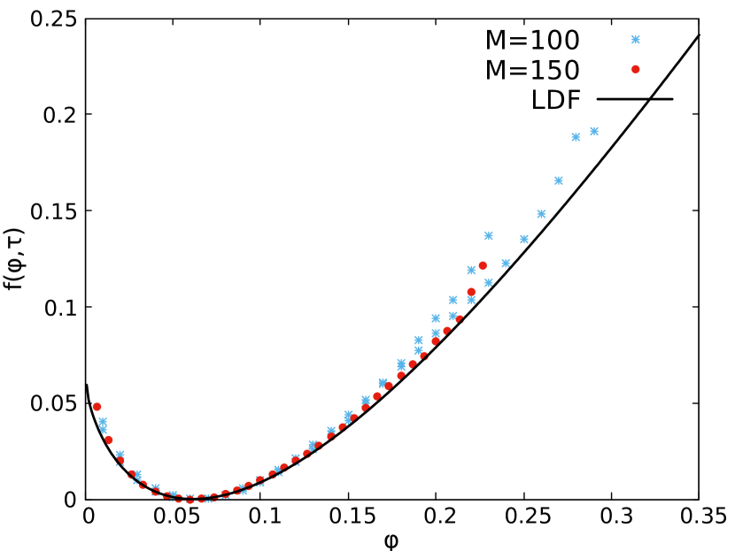
Figure S1: $f(\phi,\tau)$ with respect to $\phi$ for $\tau=3$ for $M=100,150$.

Product kernel is an exactly solvable kernel which exhibits gelation, a phenomenon in which a single macroscopic cluster with size of the order of total mass $M$ forms at $\tau>1$, and ’eats up’ the smaller clusters. The Smoluchowski equation fails when the gel appears, and the total mass is no longer conserved, necessitating the use of approximate techniques to obtain the mass distribution[1, 2]. The exact typical mass distribution for the product kernel was obtained by Lushnikov [3, 4, 5].

We now compute the LDF for the product kernel. If we proceed in the same way as we did for the constant and sum kernels, we obtain an LDF which works only within the regime where the Smoluchowski equation is valid. In order to obtain the correct LDF, we start by rewriting $H$ as given in Eq. (LABEL:eq:H') of the main text. Upon introducing coherent states and solving as before, we obtain

$$P(M,\phi,\tau_{f})\approx\lim_{M\to\infty}\sideset{}{{}^{\prime}}{\sum}_{k_{1},k_{2}\dots k_{N}=1}^{k^{*}}\exp\left[-M\left(\phi\ln\phi+1-\phi-\frac{\sum_{n=1}^{N}\ln z_{k_{n}}}{M}+\!\!\int_{0}^{\tau_{f}}\!\!d\tau\Big{[}\sum_{m}\tilde{z}_{m}\dot{z}_{m}+E\Big{]}\right)\right]\!\!,$$ (37)

where

$$H=-\frac{1}{2}\sum_{i=1}^{k^{*}}\sum_{j=1}^{k^{*}}ij\tilde{z}_{i+j}z_{i}z_{j}+\frac{1}{2}-\sum_{j=1}^{k^{*}}\frac{j^{2}\tilde{z}_{j}z_{j}}{2M^{2}}.$$ (38)

In order to compute $z_{m}(\tau)$, we solve the unscaled Euler-Lagrange equation for $z_{m}(t)$ (see Eq. (LABEL:eq:pz) of main text). Let

$$G(x,t)=\sum_{m}z_{m}(t)x^{m}.$$ (39)

Then,

$$\frac{\partial G}{\partial t}=\frac{1}{2}\left(x\frac{\partial G}{\partial x}\right)^{2}-Mx\frac{\partial G}{\partial x}+\frac{1}{2}x\frac{\partial}{\partial x}\left(x\frac{\partial G}{\partial x}\right),\leavevmode\nobreak\ \leavevmode\nobreak\ \leavevmode\nobreak\ G(x,0)=z_{1}(0)x.$$ (40)

Making the Cole-Hopf transformation $\ln D(p(x,t),t)=G(x,t)$, where $p(x,t)=xe^{-Mt}$, we obtain

$$\frac{\partial D}{\partial t}=\frac{1}{2}\frac{\partial}{\partial p}\left(p\frac{\partial D}{\partial p}\right),$$ (41)

with the initial condition $D(x,0)=e^{z_{1}(0)x}$. Let

$$D(p,t)=\sum_{m}a_{m}(t)f(m)p^{m}.$$ (42)

Then, substituting in Eq. (41) and matching the coefficients of $p^{m}$ on both sides of the equation,

$$\frac{da_{m}}{dt}=\frac{m^{2}a_{m}}{2},$$ (43)

which can be solved to obtain

$$a_{m}(t)=ce^{\frac{m^{2}t}{2}}.$$ (44)

We use the initial condition to obtain $f(m)$,

$$f(m)=\frac{z_{1}(0)^{m}}{m!}.$$ (45)

Combining Eqs. (44) and (45),

$$D(p,t)=\sum_{m}\frac{e^{\frac{m^{2}t}{2}}(z_{1}(0)p)^{m}}{m!}.$$ (46)

In order to extract $G(x,t)$ from $D(p,t)$, we use Knuth identity [6]:

$$\ln\sum_{m=1}^{\infty}\frac{x^{m(m-1)/2}z^{m}}{m!}=\sum_{m=1}^{\infty}\!\!\frac{(x-1)^{m-1}F_{m-1}(x)z^{m}}{m!},$$ (47)

where $F_{m-1}(x)$ are known as Mallows-Riordan polynomials, and obey the following recursion relation:

$$F_{m}(x)=\sum_{l=1}^{m}{m-1\choose{l-1}}\sum_{i=0}^{l-1}x^{i}F_{l-1}(x)F_{m-l}(x).$$ (48)

Converting $D(p,t)$ in terms of $x$, and equating the coefficients of $x^{m}$ on both sides of the equation, we obtain

$$z_{m}(t)=\frac{(e^{t}-1)^{m-1}F_{m-1}(e^{t})M^{m}e^{m(-Mt+t/2)}}{m!},$$ (49)

Scaling $z_{m}(t)\to z_{m}(\tau)M$ and $t\to\tau/M$, we obtain

$$z_{m}(\tau)=\frac{(e^{\tau/M}-1)^{m-1}F_{m-1}(e^{\tau/M})M^{m-1}e^{m(-\tau+\tau/2M)}}{m!}.$$ (50)

Substituting the expression for $z_{m}(\tau)$ in Eq. (LABEL:eq:actionfunctional) of the main text, we obtain the final LDF for the product kernel. Comparison with Monte Carlo results shows that the LDF is in good agreement with the simulations. Unlike the other simulations, Fig. (LABEL:fig:03)(b) for the LDF with respect to $\phi$ for $\tau=1.4$ contains simulations for small $M$ values. This is due to the limitation that the simulations are computationally expensive and consume a large amount of time. But it can be seen that even for such cases, the agreement with the analytical LDF is fairly good, and improves for larger $M$. Additionally, the LDF shows good agreement with simulation results for much larger values of $\tau$ as well, as shown in Fig. S1.

V Numerical algorithm

We briefly describe the Monte Carlo algorithm designed to numerically determine $P(M,N,t)$ for any given collision kernel. A trajectory that contributes to $P(M,N,t)$ consists of $C=M-N$ collisions, and is defined by the waiting times between collisions, sequence of collisions and the number of collisions. No collision occurs after the final waiting time. At $t=0$, there are $M$ particles of mass $1$. A trajectory is evolved by reassigning a waiting time with probability $p_{1}$, reassigning a collision with probability $p_{2}$, or modifying the number of collisions with probability $p_{3}$, such that $p_{1}+p_{2}+p_{3}=1$. Each of these moves is described below.

Reassign waiting times

: Keeping the number of collisions $C$, total time for $C$ collisions, and sequence of collisions fixed, a collision $i$ is picked at random. $\Delta t_{i}$ is the waiting time between the $i^{th}$ and $(i+1)$-th collisions, and $\lambda_{i}$ is the total rate of collision of the $i^{th}$ configuration. The waiting times $\Delta t_{i}$ and $\Delta t_{i+1}$ are modified, keeping the sum $\Delta t_{i}+\Delta t_{i+1}$ constant, such that the total time remains unchanged [7].

Reassign a collision

: Keeping the number of collisions and the total time for $C$ collisions fixed, a collision $i$ is chosen at random, and reassign according to the rules listed in [7].

Add/delete collision

: With equal probability, a collision is added or deleted.

In order to add a collision, two masses $m_{1}$ and $m_{2}$ are selected at random from the configuration resulting from the final collision. The collision rate of these masses are calculated, and used to generate the waiting time for the $(C+1)$-th collision, $\Delta t_{C+1}$.

In order to delete a collision, the final configuration is made equal to the previous one, and the waiting times are modified such that $\Delta t_{C}=\Delta t_{C}+\Delta t_{C+1}$.

Addition and deletion of a collision are performed in such a way that the principle of detailed balance is satisfied. Suppose the old trajectory consists of $C$ collisions, and the new trajectory consists of $C+1$ collisions. The probability of the old and new trajectories are $P(C)$ and $P(C+1)$ respectively, and the weights associated with adding a collision, and deleting a collision, are $Wt(C\to C+1)$ and $Wt(C+1\to C)$ respectively. The condition for detailed balance is:

$$P(C)Wt(C\to C+1)=P(C+1)Wt(C+1\to C).$$ (51)

The old trajectory has the probability

$$P(C)=\frac{1}{\lambda_{C}}\left[\prod_{i=0}^{C}\lambda_{i}e^{-\lambda_{i}\Delta t_{i}}\prod_{i=1}^{C}P(\xi_{i})\right]e^{WC},$$ (52)

where $\xi_{i}$ denote the possible configurations and $W$ is a bias parameter. The new trajectory has the probability

$$P(C+1)=\frac{1}{\lambda_{C+1}}\left[\prod_{i=0}^{C+1}\lambda_{i}e^{-\lambda_{i}\Delta t_{i}}\prod_{i=1}^{C+1}P(\xi_{i})\right]e^{W(C+1)}.$$ (53)

The protocol for adding a collision after the $C-$th collision is the following:

• Let there be L possible mass pairs which can collide, i.e., $j=1,2,\dots L$. The $j-$ th mass pair is chosen with probability

  $$\frac{K(m_{1},m_{2})n_{m_{1}}n_{m_{2}}}{\sum_{i,j}K(m_{i},m_{j})n_{m_{i}}n_{m_{j}}}.$$ (54)

• Choosing the mass pair fixes the collision rate as $\lambda^{(j)}_{C+1}$. Using this rate, we choose $\Delta t^{\prime j}_{C}$ such that $\Delta t^{\prime j}_{C}+\Delta t^{\prime}_{C+1}=\Delta t_{C}$, from the distribution

  $$P(\Delta t^{\prime j}_{C})=\frac{(\lambda^{\prime j}_{C+1}-\lambda_{C})e^{(\lambda^{\prime j}_{C+1}-\lambda_{C})\Delta t^{\prime j}_{C}}}{e^{(\lambda^{\prime j}_{C+1}-\lambda_{C})\Delta t_{C}}-1}.$$ (55)

• Now, the weight of adding a collision is

  $$Wt(C\to C+1)=P(\xi_{j})P(\Delta t^{\prime j}_{C})$$ (56)

  .

The protocol for deleting a collision just involves deleting the final configuration and setting $\Delta t_{C}=\Delta t^{\prime}_{C}+\Delta t^{\prime}_{C+1}$. That is,

$$Wt(C+1\to C)=1/\kappa,$$ (57)

where $\kappa$ is a constant.

Substituting Eqs. (52), (53), (56) and (57) into Eq. (51), we obtain

$$\kappa=\frac{\lambda_{C}e^{W}(1-e^{-(\lambda_{C+1}-\lambda_{C})\Delta t_{C}})}{\lambda_{C+1}-\lambda_{C}}.$$ (58)

That is, addition of a collision is accepted with probability $\min(\kappa,1)$, and deletion of a collision with probability $\min(1/\kappa,1)$.

Implementing the algorithm described, we see that the numerical results are in excellent agreement with the analytical LDF, as seen in Fig S1.

References

- Krapivsky et al. [2010] P. L. Krapivsky, S. Redner, and E. Ben-Naim, A kinetic view of statistical physics (Cambridge University Press, 2010).
- Leyvraz [2003] F. Leyvraz, Scaling theory and exactly solved models in the kinetics of irreversible aggregation, Physics Reports 383, 95 (2003).
- Lushnikov [2006] A. A. Lushnikov, Gelation in coagulating systems, Physica D: Nonlinear Phenomena 222, 37 (2006).
- Lushnikov [1973] A. Lushnikov, Evolution of coagulating systems, Journal of Colloid and Interface Science 45, 549 (1973).
- Lushnikov [1978] A. A. Lushnikov, Coagulation in finite systems, Journal of Colloid and interface science 65, 276 (1978).
- Knuth [1998] D. E. Knuth, Linear probing and graphs, Algorithmica 22, 561 (1998).
- Dandekar et al. [2023] R. Dandekar, R. Rajesh, V. Subashri, and O. Zaboronski, A monte carlo algorithm to measure probabilities of rare events in cluster-cluster aggregation, Computer Physics Communications 288, 108727 (2023).