Baryonic screening masses in QCD at high temperature

Abstract

We compute the baryonic screening masses with nucleon quantum numbers and its negative parity partner in thermal QCD with $N_{f}=3$ massless quarks for a wide range of temperatures, from $T\sim 1$ GeV up to $\sim 160$ GeV. The computation is performed by Monte Carlo simulations of lattice QCD with $O(a)$-improved Wilson fermions by exploiting a recently proposed strategy to study non-perturbatively QCD at very high temperature. Very large spatial extensions are considered in order to have negligible finite volume effects. For each temperature we have simulated $3$ or $4$ values of the lattice spacing, so as to perform the continuum limit extrapolation with confidence at a few permille accuracy. The degeneracy of the positive and negative parity-state screening masses, expected from Ward identities associated to non-singlet axial transformations, provides further evidence for the restoration of chiral symmetry in the high temperature regime of QCD. In the entire range of temperatures explored, the baryonic masses deviate from the free theory result, $3\pi T$, by $4$–$8\%$. The contribution due to the interactions is clearly visible up to the highest temperature considered, and cannot be explained by the expected leading behavior in the QCD coupling constant $g$ over the entire range of temperatures explored.

[a]organization=Department of Physics, University of Milano-Bicocca, addressline=Piazza della Scienza 3, postcode=20126, city=Milano, country=Italy

[b]organization=INFN, sezione di Milano - Bicocca, addressline=Piazza della Scienza 3, postcode=20126, city=Milano, country=Italy

[c]organization=Institut fur Theoretische Physik, ETH Zurich, addressline=Wolfgang-Pauli-Str. 27, city=Zurich, postcode=8093, country=Switzerland

1 Introduction

Quantum Chromodynamics (QCD) under extreme conditions is an area of intense research due to its fundamental rôle in many fields of physics, e.g. the cosmological evolution of the early universe or the interpretation of the results in relativistic heavy ion collision experiments.

It is well known that, even at very high temperatures, the perturbative approach for studying the QCD dynamics is limited by the so-called infrared problem [1]. On the one hand, finding analytic solutions to overcome this problem is by itself an interesting area of research which is being actively pursued, see Refs. [2, 3, 4, 5, 6, 7] and references therein. On the other hand, thanks to the progress achieved in lattice QCD over the last few years, it became possible to study thermal QCD non-perturbatively from first principles up to very high temperatures [8, 9].

Building on this progress, the calculation of the Equation of State (EoS) in the SU(3) gauge theory showed beyond any doubt that the contributions which are computable in perturbation theory are not enough to explain the non-perturbative result up to temperatures of at least two orders of magnitude above the critical one [10, 8]. More recently the computation of the QCD mesonic screening masses showed that the known perturbative result cannot explain their values up to temperatures of the order of the electro-weak scale or so [9]. These results point straight to the fact that, for a reliable determination of the thermal properties of QCD, a fully non-perturbative treatment of the theory is required up to temperatures of the order of the electro-weak scale or so.

The purpose of this study is to perform the first non-perturbative calculation of the baryonic screening masses with nucleon quantum numbers over a wide range of temperatures, from $T\sim 1$ GeV up to $\sim 160$ GeV. This is achieved by extending to the nucleon sector the strategy proposed in Ref. [9]. Technically this is feasible because, at asymptotically large temperatures, baryonic correlators do not suffer from the exponential depletion of the signal-to-noise ratio as they do at zero temperature [11, 12].

Baryonic screening masses are important properties of the quark-gluon plasma. They characterize the behaviour at large spatial distances of correlation functions of fields carrying baryonic quantum numbers. Being the inverse of the correlation lengths, they are related to the response of the plasma when a baryon (nucleon) is injected into the system. Screening masses are also ideal probes to verify the restoration of chiral symmetry in QCD in the high temperature regime.

While a rich literature is available on the mesonic spectrum, very few studies have been performed on the baryonic one. In particular, all lattice calculations, both in the quenched approximation [13, 14] and in the full theory [15], have been restricted to very low temperatures and no extrapolation to the continuum limit has ever been performed, see Refs. [16, 17, 18] for more recent efforts on the subject.

This letter is organized as follows. In Section 2 we introduce the definition of nucleon screening masses, and we discuss how these quantities can probe chiral symmetry restoration. In Section 3 we briefly review the strategy that we have used to simulate QCD up to the electro-weak scale, and we give the definition of the baryonic correlation functions and screening masses on the lattice. In Section 4 the values of the screening masses in the continuum limit at all temperatures considered are given. In Section 5 we discuss our final results, and present our conclusions. Various technical details are discussed in several appendices.

2 Definition of baryonic screening masses

We are interested in the screening masses related to the fermion fields

$$N\,=\,\epsilon^{abc}\left(u^{aT}C\gamma_{5}d^{b}\right)d^{c}\;,\quad\overline{N}\,=\overline{d}^{e}\left(\overline{d}^{f}C\gamma_{5}\overline{u}^{gT}\right)\epsilon^{feg}\,,$$ (1)

where the transposition acts on spinor indices, latin letters indicate color indices, and $C=i\gamma_{0}\gamma_{2}$ is the charge-conjugation matrix. The contraction with the totally anti-symmetric tensor $\epsilon^{abc}$ guarantees that the nucleon field is a color singlet.

The two-point correlation functions we are interested in are

$$C_{N^{\pm}}(x_{3})\,=\,\int dx_{0}dx_{1}dx_{2}e^{-i\frac{x_{0}}{L_{0}}\pi}\braket{\,\hbox{\rm Tr}\left[P_{\pm}N(x)\overline{N}(0)\right]}\,,$$ (2)

where $P_{\pm}=(1\pm\gamma_{3})/2$ are the projectors on positive ($N^{+}$) and negative ($N^{-}$) $x_{3}$-parity states respectively, and the trace is over the free Dirac indices of the fermion fields in Eq. (1). The integral in Eq. (2) selects the component associated to the Matsubara frequency $\pi/L_{0}$, which is the lowest one due to the anti-periodic boundary conditions of fermion fields in the compact direction of length $L_{0}$. The screening masses are defined as

$$m_{N^{\pm}}\,=\,-\lim_{x_{3}\rightarrow\infty}\frac{d}{dx_{3}}\ln\left[C_{N^{\pm}}(x_{3})\right]\,,$$ (3)

and they characterize the exponential decay of the two-point correlation functions at large spatial distances.

The comparison of $m_{N^{+}}$ with $m_{N^{-}}$ provides a quantitative test of the restoration of chiral symmetry in the high temperature regime. Indeed when chiral symmetry is not spontaneously broken, the positive and negative parity correlation functions are equal up to a sign in the chiral limit, see Eq. (19) in A, and therefore $m_{N^{+}}=m_{N^{-}}$. This is at variance of the zero temperature case, where the screening masses $m_{N^{+}}$ and $m_{N^{-}}$ correspond to the chiral limit values of the nucleon and of the $N(1535)$ masses. Due to the spontaneous breaking of chiral symmetry, they differ by several hundreds of MeV [19].

2.1 Shifted boundary conditions

In the rest of this letter, we define the thermal theory in a moving frame by requiring that the fields satisfy shifted boundary conditions in the compact direction [20, 21, 22], while we set periodic boundary conditions in the spatial directions. The former consist in shifting the fields by the spatial vector $L_{0}\,{\boldsymbol{\xi}}$ when crossing the boundary of the compact direction, with the fermions having in addition the usual sign flip. For the gluon and the quark fields these boundary conditions read

$$A_{\mu}(x_{0}+L_{0},{\boldsymbol{x}}) = A_{\mu}(x_{0},{\boldsymbol{x}}-L_{0}{\boldsymbol{\xi}})\;,$$

$$\psi(x_{0}+L_{0},{\boldsymbol{x}}) = -\,\psi(x_{0},{\boldsymbol{x}}-L_{0}{\boldsymbol{\xi}})\;,$$ (4)

$$\overline{\psi}(x_{0}+L_{0},{\boldsymbol{x}}) = -\,\overline{\psi}(x_{0},{\boldsymbol{x}}-L_{0}{\boldsymbol{\xi}})\;.$$

In the presence of shifted boundary conditions the periodic direction is identified by the vector $L_{0}(1,{\boldsymbol{\xi}})$. As a consequence, a relativistic thermal field theory in the presence of a shift ${\boldsymbol{\xi}}$ is equivalent to the very same theory with usual periodic (anti-periodic for fermions) boundary conditions but with a longer extension of the compact direction by a factor $\gamma^{-1}=\sqrt{1+\boldsymbol{\xi}^{2}}$ [22], i.e. the standard relation between the temperature and the extension in the compact direction is modified as $T^{-1}=L_{0}/\gamma=L_{0}\sqrt{1+\boldsymbol{\xi}^{2}}$. The momentum projection on the lowest Matsubara frequency has also to be modified accordingly. Thanks to the rotational symmetry of the theory, we can choose one of the axes to be in the direction of the shift, and restrict our discussion to the case ${\boldsymbol{\xi}}=(\xi,0,0)$. If we define $(x_{0},x_{1})$ the first two coordinates of a point in the system with temporal extent $L_{0}$ and shifted boundary conditions, and $(x_{0}^{\prime},x_{1}^{\prime})$ the corresponding ones in the rotated system with temporal extent $L_{0}/\gamma$ and periodic boundary conditions, the coordinates are mapped into each other by a Euclidean Lorentz transformation

$$\begin{cases}x_{0}^{\prime}\,=\,\left(x_{0}+\xi x_{1}\right)\gamma\\ x_{1}^{\prime}\,=\,\left(x_{1}-\xi x_{0}\right)\gamma\,.\end{cases}$$ (5)

The projection of the baryonic correlation function on the first Matsubara frequency is then achieved by

$$C_{N^{\pm}}(x_{3})\,=\,\int dx_{0}dx_{1}dx_{2}e^{-i\frac{x_{0}+\xi x_{1}}{L_{0}}\gamma^{2}\pi}\braket{\,\hbox{\rm Tr}\left[P_{\pm}N(x)\overline{N}(0)\right]}\,,$$ (6)

where at variance with Eq. (2), the expectation value is computed in the presence of shifted boundary conditions.

3 Lattice strategy, correlation functions and screening masses

We compute the screening masses in QCD with $N_{f}=3$ massless quarks at the $12$ temperatures $T_{0},\dots,T_{11}$ given in Table 1, i.e. for $T$ from about $1$ GeV up to approximately $160$ GeV.

We adopt shifted boundary conditions in the compact direction with ${\boldsymbol{\xi}}=(1,0,0)$ and, in order to extrapolate the results to the continuum limit with confidence, several lattice spacings are simulated at each temperature with the extension of the compact direction being $L_{0}/a=4,6,8,10$ while the length of the spatial directions is always $L/a=288$. See Appendices A and B of Ref. [9] for the details on the lattice actions and for the bare parameters of the simulations.

The key idea for reaching very high temperatures on the lattice with a moderate computational effort is to determine lines of constant physics by fixing the value of a renormalized coupling defined non-perturbatively in a finite volume [8, 9]. The coupling can be computed precisely on the lattice for values of the renormalization scale $\mu$ which span several orders of magnitude [23, 24, 25]. To make a definite choice, we adopt the definition based on the Schrödinger functional (SF) [23] for the temperatures $T_{0},\dots,T_{8}$ and on the gradient flow (GF) [26, 24, 27] for $T_{9},T_{10}$ and $T_{11}$.

$T$	$T({\rm GeV})$	$\displaystyle\frac{m_{N^{+}}}{3\pi T}$	$\displaystyle\frac{m_{N^{+}}-m_{N^{-}}}{3\pi T}$
$T_{0}$	165(6)	1.047(3)	0.0006(4)
$T_{1}$	82.3(2.8)	1.0544(19)	-0.0001(3)
$T_{2}$	51.4(1.7)	1.0569(28)	0.0002(3)
$T_{3}$	32.8(1.0)	1.0583(27)	0.0003(4)
$T_{4}$	20.6(6)	1.0596(28)	-0.0011(4)
$T_{5}$	12.8(4)	1.0662(28)	0.0001(4)
$T_{6}$	8.03(22)	1.068(3)	0.0001(6)
$T_{7}$	4.91(13)	1.075(4)	0.0004(9)
$T_{8}$	3.04(8)	1.077(4)	0.0003(9)
$T_{9}$	2.83(7)	1.076(4)	0.0009(12)
$T_{10}$	1.82(4)	1.089(4)	0.0007(20)
$T_{11}$	1.167(23)	1.078(6)	0.0016(15)

Table 1: Temperatures considered in this letter together with the best results for the nucleon mass, $m_{N^{+}}$, and the mass difference with its parity partner, $m_{N^{+}}-m_{N^{-}}$, in the continuum limit.

Once the coupling, e.g. $\bar{g}^{2}_{\rm SF}(\mu)$, is known in the continuum limit for $\mu\sim T$ [24, 25], the theory is renormalized by fixing its value at fixed lattice spacing $a$ to be

$$\bar{g}^{2}_{\rm SF}(g_{0}^{2},a\mu)=\bar{g}^{2}_{\rm SF}(\mu)\;,\quad a\mu\ll 1\;.$$ (7)

This is the condition that fixes the so-called lines of constant physics, i.e. the dependence of the bare coupling constant $g_{0}^{2}$ on the lattice spacing, for values of $a$ at which the scale $\mu$ and therefore the temperature $T$ can be easily accommodated. In other words, at different temperatures we renormalize the theory by imposing the value of the renormalized coupling constant at different scales or equivalently we impose different renormalization conditions which, however, define the very same renormalized theory at all temperatures. As a consequence, at each $T$ the theory can be simulated efficiently at various lattice spacings without suffering from large discretization errors, and the continuum limit of the observables can be taken with confidence. All technical details on how the renormalization procedure is implemented in practice are given in Appendices A and B of Ref. [9].

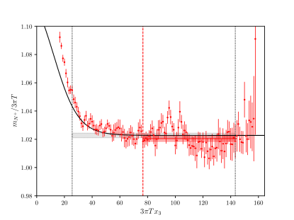
Figure 1: Plot of the effective mass $m_{N^{+}}(x_{3})$, normalized to $3\pi T$, at the temperature $T_{1}$ for $L_{0}/a=6$. For the explanation of the various fit curves and bands see the main text.

The lattice transcription of Eq. (6) for ${\boldsymbol{\xi}}=(1,0,0)$, which is the relevant case to this study, reads

$$C_{N^{\pm}}(x_{3})\, =\,a^{3}\sum_{x_{0},x_{1},x_{2}}e^{-i\frac{x_{0}+x_{1}}{2L_{0}}\pi}\braket{\,\hbox{\rm Tr}\left[P_{\pm}N(x)\overline{N}(0)\right]}\,$$

$$=\,a^{3}\sum_{x_{0},x_{1},x_{2}}e^{-i\frac{x_{0}+x_{1}}{2L_{0}}\pi}\braket{\left[W^{1}_{\pm}-W^{2}_{\pm}\right]}\,,$$ (8)

where the two terms in the second line are the Wick contractions obtained by integrating over the fermion fields. Their expressions read

$$W^{1}_{N^{\pm}}\!\! =\!\!\,\hbox{\rm Tr}\left[S^{agT}(x,0)C\gamma_{5}S^{bf}(x,0)C\gamma_{5}\right]\!\!\,\hbox{\rm Tr}\left[S^{ce}(x,0)P_{\pm}\right]\epsilon^{abc}\epsilon^{feg}\,,$$

$$W^{2}_{N^{\pm}}\!\! =\!\!\,\hbox{\rm Tr}\left[S^{agT}(x,0)C\gamma_{5}S^{be}(x,0)P_{\pm}S^{cf}(x,0)C\gamma_{5}\right]\epsilon^{abc}\epsilon^{feg},$$ (9)

where $S(x,y)$ is the quark propagator of the degenerate quarks.

Once the correlators have been computed, the effective screening masses are defined as

$$m_{N^{\pm}}(x_{3})\,=\,-\frac{1}{a}\ln\left[\frac{C_{N^{\pm}}(x_{3}+a)}{C_{N^{\pm}}(x_{3})}\right]\,.$$ (10)

As a representative example of the data, the nucleon effective mass is shown in Fig. 1 for $T_{1}$ and $L_{0}/a=6$. In order to determine the value of the screening mass, we start by fitting the effective mass to a constant plus a correction deriving from the contamination of the first excited state (solid black line) from a minimum value up to the last point where we have a good signal (black dashed lines). The minimum value is chosen to have a good quality of the fit and to have, at the same time, a non vanishing contribution from the first excited state. On one hand, for the ensembles where the signal is good enough at a large distance, from this fit we estimate the minimum value $x^{\textrm{min}}_{3}/a$ (red dashed line) from which the excited state contamination is below the target statistical precision. The screening mass is then obtained by averaging the plateau (red band) from $x^{\textrm{min}}_{3}/a$ up to the last point where we have a good signal. On the other hand, for the lowest temperatures and for the ensembles corresponding to $L_{0}/a=10$, where the loss of signal is more relevant at a large distance, the screening mass is directly estimated from the results of the effective mass fit (grey band).

Our best estimates of the screening masses are reported in Tables 2 and 3 of B for all the lattices simulated. The statistical error varies from a few permille to at most 5 permille for the smallest temperature. In order to profit from the correlations in our data for reducing the statistical errors, we also compute $(m_{N^{+}}-m_{N^{-}})/(3\pi T)$ and report its values in Tables 2 and 3 as well. This combination is particularly interesting because it is a measure of the chiral symmetry restoration which can be computed very precisely.

We have explicitly checked that finite volume effects are negligible within our statistical errors: we have generated three more lattices at the highest and at the lowest temperatures for the smallest spatial volumes corresponding to $L_{0}/a=6$, $L_{0}/a=10$, and $L_{0}/a=8$ for $T_{0}$, $T_{1}$, and $T_{11}$ respectively. These lattices have the same dimensions in the compact and in the $x_{3}$ directions as those used to extract the results in Tables 2 and 3 but smaller extensions in the other two spatial directions. The screening masses computed on them are in agreement with those calculated on the larger volume, see B for details. Therefore we can safely assume that our results have negligible finite-volume effects within the statistical precision as expected by the theoretical analysis in Ref. [9].

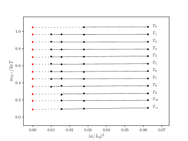
Figure 2: Numerical results for the tree-level improved nucleon screening mass at finite lattice spacing (black dots, error bars smaller than symbols). The lines in the panel represent the linear extrapolations in $(a/L_{0})^{2}$ to the continuum limit. Each temperature is analyzed independently from the others. Data corresponding to $T_{i}$ ($i=0,\dots,11$) are shifted downward by $0.09\times i$ for better readability.

4 Continuum limit of baryonic screening masses

The results that we have collected at finite lattice spacing have to be extrapolated to the continuum limit along lines of constant physics. For $O(a)$-improved actions, the Symanzik effective theory predicts the leading behaviour of the lattice artifacts to be of order $a^{2}$. We can accelerate the convergence to the continuum by introducing the tree-level improved definitions

$$m_{N^{\pm}}\longrightarrow m_{N^{\pm}}-\Big{[}m^{\rm free}_{N^{\pm}}-3\pi T\Big{]}\;,$$ (11)

where $m^{\rm free}_{N^{\pm}}$ is the mass in the free lattice theory. As shown in the D, where the computation is reported, the latter is the same for both the $m_{N^{+}}$ and the $m_{N^{-}}$ masses. From now on we will consider always the tree-level improved definition of the screening masses and indicate them with $m_{N^{\pm}}$.

All data for the improved nucleon screening mass are represented in Fig. 2 where, in order to improve the readability, data corresponding to $T_{i}$ ($i=0,\dots,11$) are shifted downward by $0.09\times i$. At each temperature, lattice artifacts are well described by a single correction proportional to $(a/L_{0})^{2}$. Indeed by fitting each data set linearly in $(a/L_{0})^{2}$, the values of $\chi^{2}/{\rm dof}$ are all around 1 with just a few outliers which, however, are not surprising given the large amount of data and fits. The results of the fits are shown in Fig. 2 as straight lines. For the mass difference $(m_{N^{+}}-m_{N^{-}})$, the coefficient of $(a/L_{0})^{2}$ is found to be compatible with zero at all temperatures. We take the continuum limit values from these fits as our best results for the nucleon screening mass and for the difference $(m_{N^{+}}-m_{N^{-}})$. They are reported in Table 1 for all the $12$ temperatures considered. As a further check of the extrapolations, we have fitted the data by excluding the coarsest lattice spacing, i.e. $L_{0}/a=4$, for the temperatures $T_{1},\ldots,T_{8}$ for which we have $4$ data points. The intercepts are in excellent agreement with those of the previous fits, albeit with a slightly larger error. For the same sets of data, we have also attempted to include in the fit a $(a/L_{0})^{2}\ln(a/L_{0})$ or a $(a/L_{0})^{3}$ term. The resulting coefficients are compatible with zero. Given the high quality of the fits and of the data, it is not necessary to model the temperature dependence of the discretization effects so as to perform a global fit of the data.

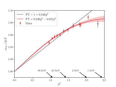
Figure 3: Nucleon screening mass versus $\hat{g}^{2}$. The band represent the best fit to Eq. (14), while the dashed line is the analytically known contribution in Eq. 13.

5 Discussion and conclusions

The main results of this paper are the baryonic screening masses reported in Table 1. They have been computed in a wide temperature range starting from $T\!\sim\!1$ GeV up to $\sim\!160$ GeV or so with a precision of a few permille.

The first observation is that, as anticipated in section 3, within our rather small statistical errors we find an excellent agreement between $m_{N^{+}}$ and $m_{N^{-}}$. This is a clear manifestation of the restoration of chiral symmetry occurring at high temperature in line with the analogous results for mesonic screening masses in Ref. [9]. For this reason in the following we discuss the nucleon mass $m_{N^{+}}$ only.

A second observation is that the bulk of the nucleon screening mass is given by the free-theory value, $3\pi T$, plus $4-8\%$ positive contribution over the entire range of temperatures explored.

To scrutinize in detail the temperature dependence induced by the non-trivial dynamics, we introduce the function $\hat{g}^{2}(T)$ defined as

$$\frac{1}{\hat{g}^{2}(T)}\equiv\frac{9}{8\pi^{2}}\ln\frac{2\pi T}{\Lambda_{\overline{\rm MS\kern-0.5pt}\kern 0.5pt}}+\frac{4}{9\pi^{2}}\ln\left(2\ln\frac{2\pi T}{\Lambda_{\overline{\rm MS\kern-0.5pt}\kern 0.5pt}}\right)\;,$$ (12)

where $\Lambda_{\overline{\rm MS\kern-0.5pt}\kern 0.5pt}=341$ MeV is taken from Ref. [30]. It corresponds to the 2-loop definition of the strong coupling constant in the $\overline{\rm MS\kern-0.5pt}\kern 0.5pt$ scheme at the renormalization scale $\mu=2\pi T$. For our purposes, however, this is just a function of the temperature $T$, suggested by the effective theory, that we use to analyze our results, see Ref. [9] for more details.

The screening masses versus $\hat{g}^{2}(T)$ are plotted in Fig. 3. The dashed line in this plot is the next-to-leading contribution to the nucleon screening mass which has been computed in the effective theory only very recently [31, 32]. For three massless quarks, the expression reads

$$\frac{m^{\rm nlo}_{N^{+}}}{3\pi T}=1+0.046g^{2}\;,$$ (13)

where $g$ is the QCD coupling constant. It is rather clear that from $T=T_{0}\sim 160$ GeV down to $T=T_{7}\sim 5$ GeV the perturbative expression is within half a percent or so with respect to the non-perturbative data. If a quick convergence of the perturbative series is assumed, this result would suggest that the bulk of the contribution due to the interactions is given by the $O(g^{2})$ term. The full set of data, however, shows a distinct negative curvature which requires higher orders in $\hat{g}^{2}$ to be parameterized. We thus fit the values of $m_{N^{+}}$ reported in the third column of Table 1 to a quartic polynomial in $\hat{g}$ of the form

$$\frac{m_{N^{+}}}{3\pi T}=b_{0}+b_{2}\,\hat{g}^{2}+b_{3}\,\hat{g}^{3}+b_{4}\,\hat{g}^{4}\;.$$ (14)

The intercept $b_{0}$ turns out to be compatible with $1$, as predicted by the free theory, within a large error. We thus enforce it to be the free-theory value, $b_{0}=1$, and we fit the data again. The coefficient of the $\hat{g}^{2}$ term turns out to be compatible with the theoretical expectation in Eq. 13 within again a large uncertainty. We have thus fixed also this coefficient to its analytical value, $b_{2}=0.046$, and we have performed again the quartic fit of the form in Eq. 14. As a result, we obtain $b_{3}=0.026(4)$, $b_{4}=-0.021(3)$ and ${\rm cov}(b_{3},b_{4})/[\sigma(b_{3})\sigma(b_{4})]=-0.99$ with $\chi^{2}/{\rm dof}=0.64$. This is indeed the best parameterization of our results over the entire range of temperatures explored.

For completeness, we notice that if the cubic coefficient is enforced to vanish, i.e. $b_{3}=0$, the fit returns $b_{2}=0.062(3)$, $b_{4}=-0.011(2)$ and ${\rm cov}(b_{2},b_{4})/[\sigma(b_{2})\sigma(b_{4})]=-0.97$ with again an excellent value of $\chi^{2}/{\rm dof}=0.68$. The coefficient $b_{2}$ , however, turns out to be in disagreement with the analytic determination. Data can also be fit to the function in Eq. 14 with $b_{0}=1$ and $b_{4}=0$ but again the coefficient $b_{2}$ would be in disagreement with the perturbative result.

Finally we observe that it has been possible to reach a precision on the nucleon screening mass of a few permille because, at asymptotically large temperatures, baryonic correlators do not suffer from the exponential depletion of the signal-to-noise ratio.

Appendix A Ward Identity in the continuum

Under the infinitesimal axial non-singlet transformation

$$\delta\psi(x)\,=\,i\epsilon\sigma_{3}\gamma_{5}\psi(x)\,,\quad\delta\overline{\psi}(x)\,=\,i\epsilon\overline{\psi}(x)\gamma_{5}\sigma_{3}\,,$$ (15)

with $\overline{\psi}=(\bar{u},\bar{d})$ and analogously for $\psi$ and where $\sigma_{3}$ is the third Pauli matrix acting on the flavour index, the nucleon fields in Eq. (1) transform as

$$\delta N(x)=-i\epsilon\gamma_{5}N(x)\;,\quad\delta\overline{N}(x)=-i\epsilon\overline{N}(x)\gamma_{5}\;.$$ (16)

If we consider the composite field

$${\cal O}(x,0)=i\,\hbox{\rm Tr}\left[\gamma_{5}P_{\pm}N(x)\overline{N}(0)\right]\,,$$ (17)

then

$$\delta{\cal O}(x,0)=\epsilon\,\hbox{\rm Tr}\left[P_{\pm}N(x)\overline{N}(0)\right]+\epsilon\,\hbox{\rm Tr}\left[P_{\mp}N(x)\overline{N}(0)\right]\;.$$ (18)

In the chiral limit, and if the symmetry is not spontaneously broken, it holds $\langle\delta{\cal O}(x,0)\rangle=0$ which in turn implies, see for instance [33] for a recent derivation,

$$\braket{\,\hbox{\rm Tr}\left[P_{+}N(x)\overline{N}(0)\right]}\,=\,-\braket{\,\hbox{\rm Tr}\left[P_{-}N(x)\overline{N}(0)\right]}\,.$$ (19)

Appendix B Simulation details and lattice results

$T$	$L_{0}/a$	$n_{\rm mdu}$	$n_{\rm nsrc}$	$\displaystyle\frac{m_{N^{+}}}{3\pi T}$​​​	$\!\!\displaystyle\frac{m_{N^{+}}\!-\!m_{N^{-}}}{3\pi T}\!\!$
$T_{0}$	4	300	4	0.9863(15)	0.0002(3)
	6	390	4	1.0178(17)	0.00041(19)
$T_{1}$	4	300	4	0.9892(18)	0.0001(3)
	6	310	4	1.0204(20)	0.0002(4)
	8	500	4	1.0371(18)	-0.00013(23)
	10	500	4	1.0438(28)	0.0003(5)
$T_{2}$	4	300	4	0.9909(23)	0.0001(4)
	6	320	4	1.0242(24)	-0.00017(28)
	8	490	4	1.0385(30)	0.00026(29)
	10	500	4	1.048(5)	0.0005(6)
$T_{3}$	4	300	4	0.9945(25)	0.0006(4)
	6	340	4	1.027(3)	0.0002(4)
	8	490	4	1.0406(23)	0.0005(3)
	10	500	4	1.048(6)	0.0003(7)
$T_{4}$	4	440	4	1.0040(16)	0.0007(5)
	6	310	4	1.0317(26)	-0.0007(4)
	8	490	4	1.0430(29)	-0.0001(4)
	10	500	4	1.054(5)	-0.0013(6)
$T_{5}$	4	310	4	1.004(3)	-0.0007(6)
	6	310	4	1.038(3)	0.0005(8)
	8	500	4	1.0466(26)	-0.0001(3)
	10	500	4	1.059(4)	-0.0001(5)
$T_{6}$	4	300	4	1.0089(25)	-0.0006(9)
	6	320	4	1.034(3)	-0.0002(7)
	8	500	4	1.054(4)	-0.0002(5)
	10	500	4	1.061(6)	0.0004(10)
$T_{7}$	4	320	4	1.012(4)	0.0005(12)
	6	310	4	1.043(4)	0.0006(7)
	8	500	4	1.059(3)	-0.0001(8)
	10	500	4	1.062(6)	0.0026(17)
$T_{8}$	4	320	8	1.016(4)	0.0023(14)
	6	300	8	1.046(4)	-0.0001(11)
	8	500	4	1.066(4)	-0.0007(8)
	10	500	5	1.061(4)	0.0013(13)

Table 2: Results for the nucleon screening mass, $m_{N^{+}}$ , and the mass difference with its parity partner, $(m_{N^{+}}-m_{N^{-}})$, normalized to $3\pi T$ at finite lattice spacing for the temperatures $T_{0},\ldots,T_{8}$. The number of molecular dynamic units (MDUs) generated, $n_{\rm mdu}$, and the number of local sources per configuration on which the two-point correlation functions have been computed, $n_{\rm nsrc}$, are also reported. The latter are always calculated by skipping $n_{\rm skip}=10$ MDUs between two consecutive measurements.

$T$	$L_{0}/a$	$n_{\rm mdu}$	$n_{\rm nsrc}$	$\;\;\;\displaystyle\frac{m_{N^{+}}}{3\pi T}$​​​	$\!\!\displaystyle\frac{m_{N^{+}}\!-\!m_{N^{-}}}{3\pi T}\!$
$T_{9}$	4	400	4	1.0180(26)	-0.0008(12)
	6	390	4	1.0526(28)	0.0005(10)
	8	390	4	1.052(5)	0.0002(10)
$T_{10}$	4	410	4	1.029(4)	-0.0019(21)
	6	400	4	1.056(3)	-0.0021(14)
	8	390	4	1.074(3)	0.0013(17)
$T_{11}$	4	400	4	1.029(4)	0.0001(21)
	6	390	4	1.055(6)	-0.0015(17)
	8	390	4	1.063(5)	0.0016(11)

Table 3: As in Table 2 but for $T_{9}$, $T_{10}$ and $T_{11}$.

We have simulated three-flavour QCD as described in Appendix E of Ref. [9]. We have accumulated a certain number of configurations for the computation of the EoS [29]. Among those, we have selected some that we have used for the computation of the screening masses. In particular in Tables  2 and 3 we report the number of MDUs considered and the number of local sources per configuration on which the two-point correlation functions have been computed. For each configuration, the best estimates of $C_{N^{\pm}}(x_{3})$ in Eq. (3) have been obtained by properly averaging their values from all local sources. The screening masses have then been extracted as described in Section 3. The results are reported in Tables 2 and 3 for the 9 highest temperatures $T_{0},\ldots$, $T_{8}$ and for the lowest ones, $T_{9}$, $T_{10}$ and $T_{11}$ respectively.

To explicitly check that finite volume effects are negligible within our statistical errors, we have generated three more lattices at $T_{0}$ ($L_{0}/a=6$), $T_{1}$ ($L_{0}/a=10$) and $T_{11}$ ($L_{0}/a=8$) at three smaller spatial volumes, namely $6\times 144^{2}\times 288$, $10\times 120^{2}\times 288$, and $8\times 144^{2}\times 288$ (direction 3 the longest) respectively. On these lattices we have computed the screening masses. They turn out to be in very good agreement with the analogous ones reported in Tables 2 and 3, and therefore they confirm the theoretical expectations that finite volume effects are negligible.

Appendix C Signal-to-noise ratio for baryon correlation functions at finite temperature

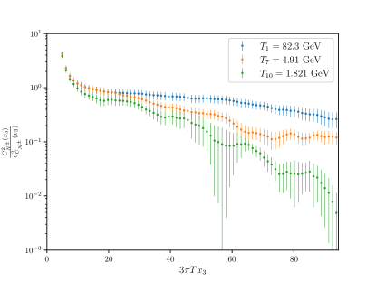
Figure 4: Signal-to-noise ratio squared at $T=T_{1}$, $T_{7}$ and $T_{10}$ for $L_{0}/a=6$.

The signal-to-noise ratio squared of baryonic correlation functions goes as

$$\frac{C^{2}_{N^{\pm}}(x_{3})}{\sigma^{2}_{C_{N^{\pm}}}(x_{3})}\propto\exp\{-(2m_{N^{\pm}}-3m_{P})x_{3}\}+\dots$$ (20)

where $\sigma^{2}_{C_{N^{\pm}}}(x_{3})$ is the variance of $C_{N^{\pm}}$ and the $\dots$ stand for sub-leading exponential contributions. At asymptotically large temperatures, and up to discretization errors, $m_{N^{\pm}}\rightarrow 3\pi T$ and $m_{P}\rightarrow 2\pi T$. As a consequence no exponential depletion of the signal-to-noise ratio with $x_{3}$ is expected when $T\rightarrow\infty$. This is at variance of what happens for $T\rightarrow 0$, where there is a severe exponential degradation of the signal-to-noise ratio because, for instance, $(2m_{N^{+}}-3m_{P})\rightarrow(2m_{N}-3m_{\pi})$ with $m_{N}$ and $m_{\pi}$ being the nucleon and the pion masses.

In Fig. 4 it is shown the signal-to-noise ratio squared for $C_{N^{+}}$ as a function of $(3\pi Tx_{3})$ for $3$ temperatures considered in this letter. As expected the depletion of the signal-to-noise ratio with $x_{3}$ becomes more severe when the temperature is lowered, and the estimate of the correlation function becomes noisier. Similar considerations apply to $C_{N^{-}}$.

Appendix D Baryonic screening masses in the free lattice theory

In order to accelerate the extrapolation to the continuum limit, we have computed the baryonic screening masses in the free theory on the lattice. In the infinite spatial volume limit, the baryonic correlation functions can be written in the form

$$C_{N^{\pm}}(x_{3})=\pm\sum_{p_{0},q_{0}}\!\!\int dp_{1}dp_{2}dq_{1}dq_{2}\mathcal{M}(p,q)e^{-2\,\Omega(p,q,k)x_{3}}\,,$$ (21)

where for shift vectors of the form ${\boldsymbol{\xi}}=(\xi,0,0)$

$$p_{0}=(2n_{0}+1)\frac{\pi}{L_{0}}-p_{1}\xi\;,\qquad n_{0}=0,\ldots,L_{0}/a-1\;,$$ (22)

analogously for $q_{0}$, and the spatial momenta are $p_{k}\in[-\pi/a,\pi/a)$. The function $\Omega(p,q,k)$ is given by

$$\Omega(p,q,k)\,=\,\hat{\omega}(p)+\hat{\omega}(q)+\hat{\omega}(k)\;$$ (23)

where $\hat{\omega}$ encodes each quark line contribution to the screening correlator as defined in Appendix F in Ref. [9], while the matrix $\mathcal{M}(p,q)$ is a calculable function of the momenta which does not play a rôle in the computation of the baryonic screening mass. For the lowest Matsubara frequency and for shift vectors of the form ${\boldsymbol{\xi}}=(\xi,0,0)$, the energy-momentum conservation implies

$$\begin{cases}p_{0}+q_{0}+k_{0}\,=\,\frac{\pi}{L_{0}}\gamma^{2}\\ p_{1}+q_{1}+k_{1}\,=\,\frac{\pi}{L_{0}}\xi\gamma^{2}\\ p_{2}+q_{2}+k_{2}\,=\,0\end{cases}\;.$$ (24)

The screening mass is obtained by minimizing $\Omega(p,q,k)$ with respect to the momenta. For the shift vector ${\boldsymbol{\xi}}=(1,0,0)$, the minimum is attained at

$$p=q=\frac{\pi}{2L_{0}}(1,1,0)\;,\qquad k=\frac{\pi}{2L_{0}}(-1,-1,0)\;.$$ (25)

Notice that, since $\hat{\omega}$ is an even function of the momenta, each quark line gives the same contribution to $\Omega$. In Table 4 we list the value of the screening mass normalized to $3\pi T$ for the temporal extents relevant to this work.

$L_{0}/a$	$m_{N^{\pm}}^{\textrm{free}}/3\pi T$
4	0.932614077…
6	0.967811412…
8	0.981401809…
10	0.987944825…

Table 4: Tree-level values of the baryonic screening mass on lattices with temporal extent $L_{0}/a$, infinite spatial volume and shift vector ${\boldsymbol{\xi}}=(1,0,0)$

References

- [1] A. D. Linde, Infrared Problem in Thermodynamics of the Yang-Mills Gas, Phys. Lett. B 96 (1980) 289–292. doi:10.1016/0370-2693(80)90769-8.
- [2] E. Braaten, R. D. Pisarski, Soft Amplitudes in Hot Gauge Theories: A General Analysis, Nucl. Phys. B337 (1990) 569–634. doi:10.1016/0550-3213(90)90508-B.
- [3] J. P. Blaizot, E. Iancu, A. Rebhan, On the apparent convergence of perturbative QCD at high temperature, Phys. Rev. D68 (2003) 025011. arXiv:hep-ph/0303045, doi:10.1103/PhysRevD.68.025011.
- [4] J. O. Andersen, M. Strickland, Resummation in hot field theories, Annals Phys. 317 (2005) 281–353. arXiv:hep-ph/0404164, doi:10.1016/j.aop.2004.09.017.
- [5] S. Mogliacci, J. O. Andersen, M. Strickland, N. Su, A. Vuorinen, Equation of State of hot and dense QCD: Resummed perturbation theory confronts lattice data, JHEP 12 (2013) 055. arXiv:1307.8098, doi:10.1007/JHEP12(2013)055.
- [6] M. Laine, A. Vuorinen, Basics of Thermal Field Theory, Vol. 925, Springer, 2016. arXiv:1701.01554, doi:10.1007/978-3-319-31933-9.
- [7] M. Arslandok, et al., Hot QCD White Paper (3 2023). arXiv:2303.17254.
- [8] L. Giusti, M. Pepe, Equation of state of the SU(3) Yang–Mills theory: A precise determination from a moving frame, Phys. Lett. B 769 (2017) 385–390. arXiv:1612.00265, doi:10.1016/j.physletb.2017.04.001.
- [9] M. Dalla Brida, L. Giusti, T. Harris, D. Laudicina, M. Pepe, Non-perturbative thermal QCD at all temperatures: the case of mesonic screening masses, JHEP 04 (2022) 034. arXiv:2112.05427, doi:10.1007/JHEP04(2022)034.
- [10] S. Borsanyi, G. Endrodi, Z. Fodor, S. Katz, K. Szabo, Precision SU(3) lattice thermodynamics for a large temperature range, JHEP 1207 (2012) 056. arXiv:1204.6184, doi:10.1007/JHEP07(2012)056.
- [11] G. Parisi, The Strategy for Computing the Hadronic Mass Spectrum, Phys. Rept. 103 (1984) 203–211. doi:10.1016/0370-1573(84)90081-4.
-
[12]
G. P. Lepage, The
Analysis of Algorithms for Lattice Field Theory, in: Boulder ASI
1989:97-120, 1989, pp. 97–120.
URL http://alice.cern.ch/format/showfull?sysnb=0117836 - [13] C. DeTar, J. B. Kogut, Measuring the hadronic spectrum of the quark plasma, Phys. Rev. D 36 (1987) 2828–2839. doi:10.1103/PhysRevD.36.2828.
- [14] A. Gocksch, P. Rossi, U. M. Heller, Quenched hadronic screening lengths at high temperature, Physics Letters B 205 (2) (1988) 334–338. doi:https://doi.org/10.1016/0370-2693(88)91674-7.
- [15] S. A. Gottlieb, W. Liu, D. Toussaint, R. L. Renken, R. L. Sugar, Hadronic Screening Lengths in the High Temperature Plasma, Phys. Rev. Lett. 59 (1987) 1881. doi:10.1103/PhysRevLett.59.1881.
- [16] S. Datta, S. Gupta, M. Padmanath, J. Maiti, N. Mathur, Nucleons near the QCD deconfinement transition, JHEP 02 (2013) 145. arXiv:1212.2927, doi:10.1007/JHEP02(2013)145.
- [17] C. Rohrhofer, Y. Aoki, G. Cossu, H. Fukaya, C. Gattringer, L. Y. Glozman, S. Hashimoto, C. B. Lang, K. Suzuki, Symmetries of the Light Hadron Spectrum in High Temperature QCD, PoS LATTICE2019 (2020) 227. arXiv:1912.00678, doi:10.22323/1.363.0227.
- [18] S. Aoki, Y. Aoki, G. Cossu, H. Fukaya, S. Hashimoto, T. Kaneko, C. Rohrhofer, K. Suzuki, Study of the axial anomaly at high temperature with lattice chiral fermions, Phys. Rev. D 103 (7) (2021) 074506. arXiv:2011.01499, doi:10.1103/PhysRevD.103.074506.
- [19] R. L. Workman, Others, Review of Particle Physics, PTEP 2022 (2022) 083C01. doi:10.1093/ptep/ptac097.
- [20] L. Giusti, H. B. Meyer, Thermodynamic potentials from shifted boundary conditions: the scalar-field theory case, JHEP 11 (2011) 087. arXiv:1110.3136, doi:10.1007/JHEP11(2011)087.
- [21] L. Giusti, H. B. Meyer, Thermal momentum distribution from path integrals with shifted boundary conditions, Phys. Rev. Lett. 106 (2011) 131601. arXiv:1011.2727, doi:10.1103/PhysRevLett.106.131601.
- [22] L. Giusti, H. B. Meyer, Implications of Poincare symmetry for thermal field theories in finite-volume, JHEP 01 (2013) 140. arXiv:1211.6669, doi:10.1007/JHEP01(2013)140.
- [23] M. Lüscher, R. Sommer, P. Weisz, U. Wolff, A precise determination of the running coupling in the SU(3) Yang-Mills theory, Nucl. Phys. B413 (1994) 481–502. arXiv:hep-lat/9309005, doi:10.1016/0550-3213(94)90629-7.
- [24] M. Dalla Brida, P. Fritzsch, T. Korzec, A. Ramos, S. Sint, R. Sommer, Determination of the QCD -parameter and the accuracy of perturbation theory at high energies, Phys. Rev. Lett. 117 (18) (2016) 182001. arXiv:1604.06193, doi:10.1103/PhysRevLett.117.182001.
- [25] M. Dalla Brida, P. Fritzsch, T. Korzec, A. Ramos, S. Sint, R. Sommer, A non-perturbative exploration of the high energy regime in QCD, Eur. Phys. J. C 78 (5) (2018) 372. arXiv:1803.10230, doi:10.1140/epjc/s10052-018-5838-5.
- [26] P. Fritzsch, A. Ramos, Studying the gradient flow coupling in the Schrödinger functional, PoS Lattice2013 (2014) 319. arXiv:1308.4559, doi:10.22323/1.187.0319.
- [27] M. Dalla Brida, P. Fritzsch, T. Korzec, A. Ramos, S. Sint, R. Sommer, Slow running of the Gradient Flow coupling from 200 MeV to 4 GeV in QCD, Phys. Rev. D 95 (1) (2017) 014507. arXiv:1607.06423, doi:10.1103/PhysRevD.95.014507.
- [28] M. Bresciani, M. Dalla Brida, L. Giusti, M. Pepe, F. Rapuano, Non-perturbative renormalization of the QCD flavour-singlet local vector current, Phys. Lett. B 835 (2022) 137579. arXiv:2203.14754, doi:10.1016/j.physletb.2022.137579.
- [29] M. Bresciani, M. Dalla Brida, L. Giusti, M. Pepe, Progresses on high-temperature QCD: Equation of State and energy-momentum tensor, PoS LATTICE2023 (2024) 192. arXiv:2312.11009, doi:10.22323/1.453.0192.
- [30] M. Bruno, M. Dalla Brida, P. Fritzsch, T. Korzec, A. Ramos, S. Schaefer, H. Simma, S. Sint, R. Sommer, QCD Coupling from a Nonperturbative Determination of the Three-Flavor Parameter, Phys. Rev. Lett. 119 (10) (2017) 102001. arXiv:1706.03821, doi:10.1103/PhysRevLett.119.102001.
- [31] L. Giusti, M. Laine, D. Laudicina, M. Pepe, P. Rescigno, Baryonic thermal screening mass at NLO, to appear (2024).
- [32] T. H. Hansson, M. Sporre, I. Zahed, Baryonic and gluonic correlators in hot QCD, Nucl. Phys. B 427 (1994) 545–560. arXiv:hep-ph/9401281, doi:10.1016/0550-3213(94)90639-4.
- [33] G. Aarts, C. Allton, D. De Boni, S. Hands, B. Jäger, C. Praki, J.-I. Skullerud, Light baryons below and above the deconfinement transition: medium effects and parity doubling, JHEP 06 (2017) 034. arXiv:1703.09246, doi:10.1007/JHEP06(2017)034.