Constraining the mass-spectra in the presence of a light sterile neutrino from absolute mass-related observables

Abstract

The framework of three-flavor neutrino oscillation is a well-established phenomenon, but results from the short-baseline experiments, such as the Liquid Scintillator Neutrino Detector (LSND) and MiniBooster Neutrino Experiment (MiniBooNE), hint at the potential existence of an additional light neutrino state characterized by a mass-squared difference of approximately $1\,\rm eV^{2}$. The new neutrino state is devoid of all Standard Model (SM) interactions, commonly referred to as a “sterile” state. In addition, a sterile neutrino with a mass-squared difference of $10^{-2}$ $\rm eV^{2}$ has been proposed to improve the tension between the results obtained from the Tokai to Kamioka (T2K) and the NuMI Off-axis $\nu_{e}$ Appearance (NO$\nu$A) experiments. Further, the non-observation of the predicted upturn in the solar neutrino spectra below 8 MeV can be explained by postulating an extra light sterile neutrino state with a mass-squared difference around $10^{-5}\,\rm eV^{2}$. The hypothesis of an additional light sterile neutrino state introduces four distinct mass spectra depending on the sign of the mass-squared difference. In this paper, we discuss the implications of the above scenarios on the observables that depend on the absolute mass of the neutrinos, namely - the sum of the light neutrino masses $(\Sigma)$ from cosmology, the effective mass of the electron neutrino from beta decay $(m_{\beta})$, and the effective Majorana mass $(m_{\beta\beta})$ from neutrinoless double beta decay. We show that some scenarios can be disfavored by the current constraints of the above variables. The implications for projected sensitivity of Karlsruhe Tritium Neutrino Experiment (KATRIN) and future experiments like Project-8, next Enriched Xenon Observatory (nEXO) have been discussed.

I Introduction

The phenomena of neutrino oscillations, in which neutrino flavor states switch their identities while propagating, have been observed in several terrestrial experimentsSuper-Kamiokande:1998kpq ; SNO:2002tuh ; KamLAND:2002uet ; MINOS:2006foh . This requires at least two of the neutrinos to have small but non-zero masses and mixing between the different flavors. This, in turn, implies physics beyond the Standard Model (SM). Many BSM scenarios have been studied for generating neutrino masses. The smallness of the neutrino masses is often linked with lepton number violation through the dimension 5 Weinberg operator $\frac{LLHH}{\Lambda}$ Weinberg:1979sa . This operator violates the lepton number, which signifies the Majorana nature of the neutrinos.

Neutrino oscillation experiments are sensitive to two mass-squared differences and mixing angles of the neutrinos. However, they cannot shed light on the absolute mass scale or the nature of neutrinos. If neutrinos are considered to be Majorana in nature, a rare and slow nuclear decay, known as neutrinoless double beta decay ($0\nu\beta\beta$) Furry:1939qr , can exist in nature. Several experiments aimed to observe this process, but there has not been any positive evidence so far. The KamLAND-Zen experiment using the Xe¹³⁶ isotope as the decaying nucleus gives the lower bound on the half-live as $T_{1/2}^{0\nu\beta\beta}>1.07\times 10^{26}$ yr at 90% confidence level Shirai:2018ycl whereas the GERDA experiment uses Ge⁷⁶ isotope and their latest limit on the half-life is $T_{1/2}^{0\nu\beta\beta}>1.8\times 10^{26}$ yr at 90% confidence level GERDA . The lower bounds on half-lives can be translated into upper bounds on the effective Majorana mass parameter ($m_{\beta\beta}$), which depends on the neutrino masses, mixing angles, and the Majorana phases.

The information about the absolute mass scale of neutrinos can also come from tritium beta decay. The KATRIN experiment sets the current limit on the mass parameter, $m_{\beta}\lesssim 0.8\,\rm eV$ at 90% confidence level KATRIN:2021uub .

Cosmological observations like CMB anisotropies, large-scale structure formation, etc., can also put bound on the absolute mass scale of neutrinos. The most stringent bound on the sum of the light neutrino masses ($\Sigma$) $<\,0.12\rm\,eV$ comes from the Planck collaboration by considering three degenerate neutrino mass eigenstates Planck:2018vyg .

Although the three-generation paradigm is well established, there are experimental anomalies that indicate the presence of an extra light sterile neutrino of mass of the order of eV. The short baseline experiments, LSNDLSND:2001aii and MiniBooNE MiniBooNE:2020pnu , showed an excess signature of electron neutrinos coming from a muon neutrino beam. Gallium-based solar neutrino experiments GALLEXGALLEX:1997lja , SAGE Abdurashitov:1996dp , & as well as the BESTBarinov:2021asz experiments found the deficit in electron neutrinos while calibrating the detector using the neutrinos from ${}^{51}Cr$ source. One possible resolution of the results from these experiments is provided by incorporating an additional light neutrino state with mass $\sim 1$ eV. There are also motivations for considering sterile neutrinos lower than the eV scale. The inclusion of a sterile neutrino with mass squared difference ($\Delta m_{s}^{2}$ )$\sim 10^{-5}\,\rm eV^{2}$ has been postulated deHolanda:2010am to explain the absence of the upturn of solar neutrino probability below 8 MeV. Additionally, it is also shown that the tension between $NO\nu A$ and $T2K$ data can be reduced in the presence of a sterile neutrino with $\Delta m_{s}^{2}\sim(10^{-4}:10^{-2})$ eV². Recently, the signatures of the sub-eV sterile neutrinos in future experiments have been studied in the references KumarAgarwalla:2019blx ; Agarwalla:2018nlx ; Chatterjee:2023qyr ; Chatterjee:2022pqg in the context of future long baseline atmospheric neutrino experiments.

In this paper, we study the implication of a very light sterile neutrino with $\Delta m_{s}^{2}$ in the range ($10^{-4}:10^{-2}$) eV² on the mass-related variables such as $m_{\beta\beta},m_{\beta},$ and $\Sigma$. Such investigations in the context of an eV scale sterile neutrino have been explored in Goswami:2005ng . In our work, along with the sub-eV scale sterile neutrino we also present the results for an eV scale sterile neutrino with the current constraints on the mixing the parameters. We consider the 3+1 picture with a single sterile neutrino added to the three sequential neutrinos. In this case, there can be four mass possible spectra; two each with $\Delta m_{s}^{2}>0$ and $\Delta m_{s}^{2}<0$. We explore the implication of the cosmological constraint on the sum of light neutrino masses for these spectra. We also discuss the constraints on the possible mass spectra in the light of KATRIN results on $m_{\beta}$ and KamLAND-Zen results on $m_{\beta\beta}$. Additionally, we examine the implications of the future measurements by proposed experiments Project8, nEXO.

The plan of the paper is as follows. Section 2 gives a brief overview of the neutrino mass and mixing scenarios in the standard three-generation and 3+1 framework. In section 3, we study the implications of the various mass spectra for $\Sigma$, $m_{\beta\beta}$, and $m_{\beta},$. Section 4 presents an analysis on the correlation between $m_{\beta\beta},m_{\beta},$ and $\Sigma$. Finally, we summarize the results in section 5.

II Neutrino Masses and Mixing

II.1 The Standard framework

Neutrino oscillation is governed by the Pontecorvo-Maki-Nakagawa-Sakata (PMNS) matrix (U), which describes the relationship between the neutrino flavor and mass eigenstates Maki:1962mu . The mass matrix in the flavour basis $\mathcal{M}_{\nu}$ and the mass matrix in the mass basis $M_{\nu}^{\rm diag}$ are related as,

$$\mathcal{M}_{\nu} = U\,M_{\nu}^{\rm diag}\,U^{T},$$ (1)

$$\text{where }\quad M_{\nu}^{\rm diag} = \rm{diag}\,\left(m_{1},m_{2},m_{3}\right)\,,$$ (2)

The PMNS matrix is parameterized by three mixing angles $(\theta_{12}\,,\,\theta_{13}\,,\,\theta_{23})$ and one CP Phase $(\delta_{13})$ for Dirac neutrinos, whereas Majorana nature of neutrino adds two extra phases $(\alpha,\,\beta)$ along with it. Various oscillation experiments provide information about the mixing angles ($\theta_{12},\theta_{13},\theta_{23}$) and mass-squared differences ($\Delta m_{\rm sol}^{2}\,,\,\Delta m_{\rm atm}^{2}$). Here $\Delta m_{\rm sol}^{2}\,>\,0$ and defined as $m_{2}^{2}-m_{1}^{2}$. Depending on the sign of $\Delta m_{\rm atm}^{2}$, the masses in the three flavor framework are categorized into two mass orderings

• Normal Ordering (NO): In NO, $\Delta m_{\rm atm}^{2}\equiv m_{3}^{2}-m_{1}^{2}>0$. The mass ordering in this scenario is $m_{1}<m_{2}<m_{3}$, and the mass relations can be expressed as

  $$m_{\rm lightest} = m_{1},\quad m_{2}=\sqrt{m_{1}^{2}+\Delta m_{\rm sol}^{2}},\quad m_{3}=\sqrt{m_{1}^{2}+\Delta m_{\rm atm}^{2}}$$ (3)

• Inverted Ordering (IO): In this case, the mass ordering is $m_{3}<m_{1}<m_{2}$ and $\Delta m_{\rm atm}^{2}\equiv m_{3}^{2}-m_{2}^{2}\,<\,0$. In this ordering, the mass relation ns are written as,

  $$m_{\rm lightest} = m_{3},\quad m_{2}=\sqrt{m_{3}^{2}+\Delta m_{\rm atm}^{2}},\quad m_{1}=\sqrt{m_{3}^{2}+\Delta m_{\rm atm}^{2}-\Delta m_{\rm sol}^{2}}$$ (4)

• Quasi Degenerate Spectrum (QD): Apart from NO and IO, there might be a scenario where $m_{1}\approx m_{2}\approx m_{3}$. This scenario is generally referred to as quasi degenerate spectrum. In this scenario, the value of the lightest mass is greater than $\sqrt{\Delta m_{\rm atm}^{2}}$.

The current best fit and $3\sigma$ range of these parameters, determined from various experiments, are given in table (1).

Table 1: $3\sigma$ ranges and best fit values extracted of three neutrino oscillation parameters Esteban:2020cvm . Here, $\Delta m_{\rm sol}^{2}\,\equiv\,m_{2}^{2}-m_{1}^{2}$ and $\Delta m_{\rm atm}^{2}\,\equiv\,m_{3}^{2}-m_{1}^{2}$ for NO and $m_{2}^{2}-m_{3}^{2}$ for IO.

Parameters	Normal Ordering		Inverted Ordering
	$3\sigma$ range	Best Fit	$3\sigma$ range	Best Fit
$\sin^{2}\theta_{12}$	$0.270:0.341$	0.303	$0.270:0.341$	0.303
$\theta_{12}$	$31.31^{\circ}:35.74^{\circ}$	$33.41^{\circ}$	$31.31^{\circ}:35.74^{\circ}$	$33.41^{\circ}$
$\sin^{2}\theta_{13}$	$0.0202:0.0239$	0.0220	$0.0202:0.0239$	0.0220
$\theta_{13}$	$8.19^{\circ}-8.89^{\circ}$	$8.54^{\circ}$	$8.23^{\circ}:8.90^{\circ}$	$8.57^{\circ}$
$\sin^{2}\theta_{23}$	$0.406:0.620$	0.572	$0.412:0.623$	0.578
$\theta_{23}$	$39.6^{\circ}:51.9^{\circ}$	$49.1^{\circ}$	$39.9^{\circ}:52.1^{\circ}$	$49.5^{\circ}$
$\delta_{13}$	$197^{\circ}$	$108^{\circ}:404^{\circ}$	$286^{\circ}$	$192^{\circ}:360^{\circ}$
$\Delta m^{2}_{\rm sol}/10^{-5}{\rm eV}^{2}$	$6.82:8.03$	$7.41$	$6.82:8.03$	$7.41$
$\Delta m^{2}_{\rm{atm}}/10^{-3}{\rm eV}^{2}$	$2.428:2.597$	$2.511$	$(-2.581:-2.408)$	$-2.498$

II.2 The 3+1 framework

In this case, we have one extra mass-squared difference ($\Delta m_{s}^{2}\equiv m_{4}^{2}-m_{1}^{2}$), three new mixing angles $(\theta_{14}\,,\,\theta_{24}\,\,\theta_{34})$ and two new Dirac CP phases $(\delta_{14}\,,\,\delta_{24})$ and one additional Majorana phase $(\gamma)$. The mass matrix in the flavor basis can be defined as,

$$\mathcal{M}^{s}_{\nu} = U\,M_{\nu}^{\rm diag}\,U^{T},\quad\text{where }\quad M_{\nu}^{\rm diag}=\rm{diag}\,\left(m_{1},m_{2},m_{3},m_{4}\right)$$ (5)

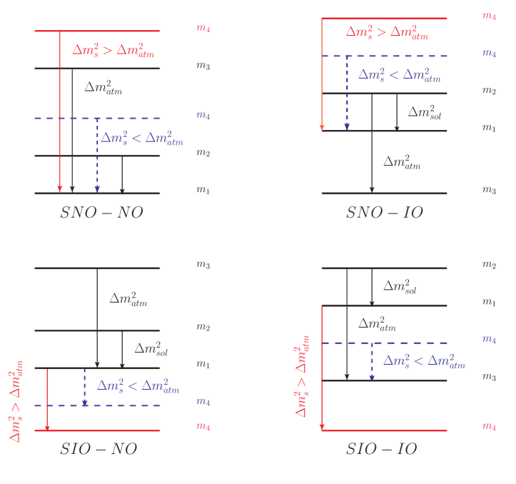
Figure 1: Possible mass spectra with the inclusion of a sterile neutrino. Here red solid line corresponds to the value of $m_{4}$ when $\Delta m_{s}^{2}>\Delta m_{\rm atm}^{2}$ whereas the blue dashed line indicates the same with $\Delta m_{s}^{2}<\Delta m_{\rm atm}^{2}$

In the 3+1 framework, the mixing matrix $U$ can be parameterized as,

$$U = R_{34}(\theta_{34})\,\tilde{R}_{24}(\theta_{24},\delta_{24})\,\tilde{R}_{14}(\theta_{14},\theta_{14})\,R_{23}(\theta_{23})\,\tilde{R}_{13}(\theta_{13},\delta_{13})\,R_{12}(\theta_{12})\,P$$ (6)

$$= \begin{pmatrix}U_{e1}&U_{e2}&U_{e3}&U_{e4}\\ U_{\mu 1}&U_{\mu 2}&U_{\mu 3}&U_{\mu 4}\\ U_{\tau 1}&U_{\tau 2}&U_{\tau 3}&U_{\tau 4}\\ U_{s1}&U_{s2}&U_{s3}&U_{s4}\end{pmatrix}$$

where $R_{ij}$’s are the standard rotational matrices in the $i,j$ generational space. For instance

$$R_{34}(\theta_{34}) = \begin{pmatrix}1&0&0&0\\ 0&1&0&0\\ 0&0&c_{34}&s_{34}\\ 0&0&-s_{34}&c_{34}\end{pmatrix},\quad\tilde{R}_{14}(\theta_{14},\delta_{14})=\begin{pmatrix}c_{14}&0&0&s_{14}\,e^{-i\,\delta_{14}}\\ 0&1&0&0\\ 0&0&1&0\\ -s_{14}\,e^{i\,\delta_{14}}&0&0&c_{14}\end{pmatrix}$$ (7)

Table 2: Allowed values of the sterile neutrino parameters $\Delta m^{2}_{s},\,\sin^{2}\theta_{14}$ in the 3+1 scenario for three different mass squared differences ($\Delta m_{s}^{2}=10^{-4}\,\rm eV^{2}\,,\,0.01\,\rm eV^{2}$ and $1.3\,\rm eV^{2}$) are given. The value of the $\sin^{2}\theta_{14}$ is chosen to be consistent with MINOS , MINOS⁺, Daya-Bay and Bugey-3 data MINOS:2017cae

Parameters	Case I	Case II	Case III
$\Delta m_{s}^{2}$	$10^{-4}\,\rm eV^{2}$	$10^{-2}\,\rm eV^{2}$	$1.3\,\rm eV^{2}$
$\sin^{2}\theta_{14}$	$0.1\,:\,0.2$	$5\times 10^{-4}\,:\,5\times 10^{-3}$	$0.001\,:\,0.01$

Here, $c_{ij}(s_{ij})$ stands for $\cos\theta_{ij}\,(\sin\theta_{ij})$ and $P$ is the diagonal matrix containing the Majorana phases, defined as $P=\text{diag}\,\left(1,\,e^{i\frac{\alpha}{2}},\,e^{i\left(\frac{\beta}{2}+\delta_{13}\right)},\,e^{i\left(\frac{\gamma}{2}+\delta_{14}\right)}\right)$. In table (2), we present three representative values of $\Delta m_{s}^{2}$ and $\sin^{2}\theta_{14}$ extracted from the allowed region from MINOS , MINOS⁺, Daya-Bay  and Bugey-3 experimentsMINOS:2017cae ; Acero:2022wqg . The value of $\sin^{2}\theta_{14}$ analysing the LSND and MiniBooNE data is in the range $(0.01:0.02)$ for $\Delta m_{s}^{2}$ = 1.3 $\rm eV^{2}$, whereas the MINOS , MINOS⁺ data allows the region with $\sin^{2}\theta_{14}$ is $<0.01$.

In the 3+1 framework, the sign and the magnitude of $\Delta m_{s}^{2}$ lead to different mass spectra.

1. SNO-NO $\bf(\Delta m_{s}^{2}>0\,,\,\Delta m_{\rm atm}^{2}>0\,)$:
   In this scenario, mass ordering is different for $\Delta m_{s}^{2}>\Delta m_{\rm atm}^{2}$ and $\Delta m_{s}^{2}<\Delta m_{\rm atm}^{2}$ which is depicted in the top left corner of Fig. (1) with a red solid line and a blue dashed line respectively. For $\Delta m_{s}^{2}>\Delta m_{\rm atm}^{2}$, the mass ordering is $m_{1}<m_{2}<m_{3}<m_{4}$, given in the top left corner of Fig. (1). Whereas for $\Delta m_{s}^{2}<\Delta m_{\rm atm}^{2}$, the ordering is $m_{1}<m_{2}<m_{4}<m_{3}$. In both cases, the mass relations are expressed as

   $$m_{\text{lightest}}=m_{1},\quad\quad m_{2} = \sqrt{m_{1}^{2}+\Delta m_{\rm sol}^{2}}$$

   $$m_{3}=\sqrt{m_{1}^{2}+\Delta m_{\rm atm}^{2}},\quad\quad m_{4} = \sqrt{m_{1}^{2}+\Delta m_{s}^{2}}$$ (8)

2. SNO-IO $\bf(\Delta m_{s}^{2}>0\,,\,\Delta m_{\rm atm}^{2}<0\,)$ :
   In this case, the mass ordering is the same for both $\Delta m_{s}^{2}>\Delta m_{\rm atm}^{2}$ and $\Delta m_{s}^{2}<\Delta m_{\rm atm}^{2}$ and is delineated as $m_{3}<m_{1}<m_{2}<m_{4}$. The mass relations are expressed as

   $$m_{\text{lightest}}=m_{3},\quad\quad m_{2} = \sqrt{m_{3}^{2}+\Delta m_{\rm atm}^{2}}$$

   $$m_{1}=\sqrt{m_{3}^{2}+\Delta m_{\rm atm}^{2}+\Delta m_{\rm sol}^{2}},\quad\quad m_{4} = \sqrt{m_{3}^{2}+\Delta m_{\rm atm}^{2}-\Delta m_{\rm sol}^{2}+\Delta m_{s}^{2}}$$ (9)

3. SIO-NO $\bf(\Delta m_{s}^{2}<0\,,\,\Delta m_{\rm atm}^{2}>0\,)$ :
   The mass ordering in this scenario is defined as $m_{4}<m_{1}<m_{2}<m_{3}$, and it is the same for both the $\Delta m_{s}^{2}$ ranges. The mass relations can be written as,

   $$m_{\text{lightest}}=m_{4},\quad\quad m_{2} = \sqrt{m_{4}^{2}+\Delta m_{s}^{2}+\Delta m_{\rm sol}^{2}}$$

   $$m_{1}=\sqrt{m_{4}^{2}+\Delta m_{s}^{2}},\quad\quad m_{3} = \sqrt{m_{4}^{2}+\Delta m_{s}^{2}+\Delta m_{\rm atm}^{2}}$$ (10)

4. SIO-IO $\bf(\Delta m_{s}^{2}<0\,,\,\Delta m_{\rm atm}^{2}<0\,)$ :
   

   • For $\Delta m_{s}^{2}>\Delta m_{\rm atm}^{2}$, the mass ordering is $m_{4}<m_{3}<m_{1}<m_{2}$ and the mass relations are defined as :

     $$m_{\text{lightest}}=m_{4},\quad\quad m_{2} = \sqrt{m_{4}^{2}+\Delta m_{s}^{2}+\Delta m_{\rm sol}^{2}}$$

     $$m_{1}=\sqrt{m_{4}^{2}+\Delta m_{s}^{2}},\quad\quad m_{3} = \sqrt{m_{4}^{2}+\Delta m_{s}^{2}+\Delta m_{\rm sol}^{2}-\Delta m_{\rm atm}^{2}}$$ (11)

   • For $\Delta m_{s}^{2}<\Delta m_{\rm atm}^{2}$, the mass ordering is $m_{3}<m_{4}<m_{1}<m_{2}$ and the mass relations can be expressed as :

     $$m_{\text{lightest}}=m_{3},\quad\quad m_{2} = \sqrt{m_{3}^{2}+\Delta m_{\rm atm}^{2}}$$

     $$m_{1}=\sqrt{m_{3}^{2}+\Delta m_{\rm atm}^{2}-\Delta m_{\rm sol}^{2}},\quad\quad m_{4} = \sqrt{m_{3}^{2}+\Delta m_{\rm atm}^{2}-\Delta m_{\rm sol}^{2}-\Delta m_{s}^{2}}$$

     In the appendix, we have given the variation of masses ($m_{i}$) with respect to the lightest mass for all the scenarios.

III Neutrino mass variables

In this section, we study the implications of adding an additional sterile neutrino for the mass variables $m_{\beta\beta},m_{\beta},\Sigma$.

III.1 Bound from cosmology

Light sterile neutrinos can have a significant impact on the evolution of the universe, and thus, their presence can be investigated using cosmological observations. If sterile neutrinos are massless, they contribute to the light relativistic degrees of freedom in the early universe, quantified as $N_{\rm eff}$, which can be directly constrained from Cosmic Microwave Background (CMB) and Large Scale Structure (LSS) data. The Standard Model of particle physics predicts $N^{\rm SM}_{\rm eff}=3.044^{+0.0002}_{-0.0002}$ Bennett:2020zkv , assuming only three degenerate light active neutrinos, but can increase in general when the sterile neutrino contribution is added.

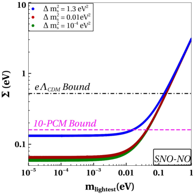
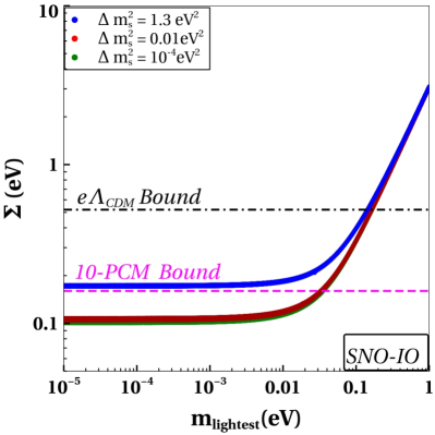
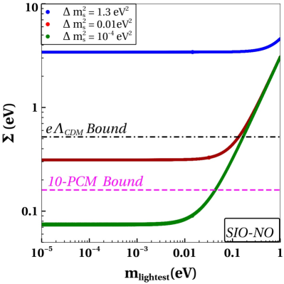
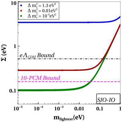
Figure 2: The variation total effective mass $\Sigma$ with the lightest neutrino mass $m_{\rm lightest}$ in different scenarios SNO-NO (top-left), SNO-IO (top-right), SIO-NO (bottom-left), and SIO-IO (bottom-right). The green, red, and blue colors correspond to $\Delta m_{s}^{2}=10^{-4}\,\rm eV^{2},0.01\,eV^{2},1.3$ eV², respectively. The magenta dashed line corresponds to the 10 parameter cosmological (10-PCM) model and the black dashed-dot line corresponds to the extended $\Lambda_{CDM}$ ($e\Lambda_{CDM}$)bound.

In the case of massive sterile neutrinos, one needs to add one more free parameter, $m_{s}^{\rm eff.}$, the effective sterile neutrino mass in the cosmological models along with $N_{\rm eff}$. The effective sterile neutrino mass is different from its physical mass ($m^{\rm ph}_{s}$) but can be related as $m_{s}^{\rm eff}\,=\,\Delta N_{\rm eff}^{3/4}\,m_{s}^{\rm ph}$ if the neutrinos are fully thermalized with active neutrinos and $m_{s}^{\rm eff}\,=\,\Delta N_{\rm eff}\,m_{s}^{\rm ph}$ for the partially thermalized sterile neutrinos where $\Delta N_{\rm eff}=N_{\rm eff}-N_{\rm eff}^{\rm SM}$.

When PLANK 2018 data is fitted with standard $\Lambda_{\rm CDM}$ cosmological model, it tends to disfavor the presence of extra light relativistic degrees of freedom Planck:2018vyg . However, with the inclusion of more parameters with the standard $\Lambda_{\rm CDM}$ cosmological model and fitting more data from different cosmological observations, the cosmological constraints can be relaxed. For example, in a recent analysis, the Plank + BAO + Hubble parameter measurement Riess:2018uxu + Supernova Ia Pan-STARRS1:2017jku data fitted with a 10 parameter cosmological model (10-PCM) i.e $\Lambda_{CDM}+N_{\rm eff}+m^{s}_{\rm eff}+w_{0}+n_{run}$, gives the constraints on $N_{\rm eff}$ and $\Sigma$ as follows Acero:2022wqg ,

$$N_{\rm eff}=3.11^{+0.37}_{-0.36},\,\,\,\Sigma=0.16\,\rm eV$$ (13)

where $\omega_{0}$ is the equation of state parameter of the dark energy and $n_{run}$ is the running of the scalar spectral index, a parameter related to the initial conditions of the universe. Another model with 12 parameters, called extended $\Lambda_{\rm CDM}$ ($e\Lambda_{\rm CDM}$) gives bound as ,

$$N_{\rm eff}=3.11^{+0.52}_{-0.48},\,\,\,\Sigma=0.52\rm\,eV$$ (14)

where, $\Sigma$ is defined as Hagstotz:2020ukm

$$\Sigma=m_{1}+m_{2}+m_{3}+m_{s}^{\rm eff}$$ (15)

A fully thermalized neutrino implies $\Delta N_{\rm eff}\approx 1$, which is ruled out from the cosmological data. Here, we have considered the sterile neutrino to be produced non-thermally which means that $m_{s}^{\rm eff}=\Delta N_{\rm eff}\,m_{4}$, $m_{4}$ is the physical mass of the sterile neutrino. We have plotted $\Sigma$ as a function of the lightest neutrino mass for different mass schemes in Fig. (2) assuming the value of $N_{\rm eff}=3.11$ from Eqn. (13), (14). The pink dashed line indicates the limit $\Sigma=\,0.16\,\rm eV$, and the black dashed-dot line corresponds to $\Sigma=0.52\,\rm eV$.

The important features observed from Fig. (2) are as follows,

• The SNO-NO scenario is favored by $e\Lambda_{\rm CDM}$ model up to $m_{\rm lightest}\sim 0.15$ eV for all the three mass-squared differences. Whereas the 10-PCM is more constraining and disfavor $\Delta m_{s}^{2}=1.3\,\rm eV^{2}$ above $m_{\rm lightest}>0.01\,\rm eV$ and $\Delta m_{s}^{2}=10^{-4}\,\rm eV^{2}\,,\,0.01\,\rm eV^{2}$ above $m_{\rm lightest}>0.04\,\rm eV$.

• For SNO-IO, $e\Lambda_{\rm CDM}$ model allows all values of $\Delta m_{s}^{2}$ up to $m_{\rm lightest}\sim 0.15$ eV. However, $\Delta m_{s}^{2}=1.3$ eV² is disfavored by the 10-PCM for the entire range of $m_{\rm lightest}$. The lower values of $\Delta m_{s}^{2}$ are still allowed up to $m_{\rm lightest}\sim 0.04\,\rm eV$.

• For SIO-NO and SIO-IO, the 10-PCM disfavors $\Delta m_{s}^{2}=0.01\,\rm eV^{2}$ and $1.3\,\rm eV^{2}$ for the entire range of $m_{\rm lightest}$ but $\Delta m_{s}^{2}=10^{-4}\,\rm eV^{2}$ is still allowed up to $m_{\rm lightest}\sim 0.03\,\rm eV$. However, if we consider $e\Lambda_{\rm CDM}$ model, then $\Delta m_{s}^{2}=0.01\,\rm eV^{2}$ gets allowed up to $m_{\rm lightest}\sim 0.1\,\rm eV$.

The above discussion is summarised in table (3).

Table 3: The table summarises the status of four mass spectra for three different $\Delta m_{s}^{2}$ in the light of different cosmological models. The limits correspond to the value of $m_{\rm lightest}$ up to which the scenario is allowed.

Mass ordering ($m_{\rm lightest})$	$\Delta m_{s}^{2}=10^{-4}\,\rm eV^{2}$		$\Delta m_{s}^{2}=0.01\,\rm eV^{2}$		$\Delta m_{s}^{2}=1.3\,\rm eV^{2}$
	Limit $\quad 10-\rm PCM$	Limit e$\Lambda_{\rm CDM}$	Limit $\quad 10-\rm PCM$	Limit $e\Lambda_{\rm CDM}$	Limit $\quad 10-\rm PCM$	Limit e$\Lambda_{\rm CDM}$
SNO-NO ($m_{1}$)	$<0.04$	$<0.15$	$<0.04$	$<0.15$	$<0.01$	$<0.15$
SNO-IO ($m_{3}$)	$<0.03$	$<0.1$	$<0.03$	$<0.1$	Disallowed	$<0.1$
SIO-NO ($m_{4}$)	$<0.04$	$<0.1$	Disallowed	$<0.1$	Disallowed	Disallowed
SIO-IO ($m_{3}/m_{4}$)	$<0.04$	$<0.1$	Disallowed	$<0.1$	Disallowed	Disallowed

III.2 Bound from Tritium $\beta$ decay

A direct and model-independent constraint on the neutrino mass can be derived through the experimental analysis of the electron energy spectrum resulting from beta decay in atomic nuclei. In beta decay, the energy excess due to the nuclear mass difference is shared among the electron, (anti)neutrino and the daughter nucleus. If the energy resolution of the experiment exceeds the splittings of the neutrino mass states ($\Delta E>>m_{i}$) then the emitted electron’s spectrum depends on a quantity called the “kinematic mass” of the electron neutrino which is defined as

$$m_{\beta} = \sqrt{\left|U_{e1}\right|^{2}m_{1}^{2}+\left|U_{e2}\right|^{2}m_{2}^{2}+\left|U_{e3}\right|^{2}m_{3}^{2}+\left|U_{e4}\right|^{2}m_{4}^{2}}$$ (16)

$$= \sqrt{c_{12}^{2}c_{13}^{2}c_{14}^{2}m_{1}^{2}+s_{12}^{2}c_{13}^{2}c_{14}^{2}m_{2}^{2}+s_{13}^{2}c_{14}^{2}m_{3}^{2}+s_{14}^{2}m_{4}^{2}}$$

The kinematic mass depends on the mixing parameters, mass squared differences, and the lightest neutrino mass. The current KATRIN limit on $m_{\beta}$ is $\leq\,0.8\,\rm eV$ and the future sensitivity is quoted as $m_{\beta}\leq\,0.2\,\rm eV$. We have plotted $m_{\beta}$ as a function of the lightest neutrino mass in Fig. (3) by varying all the parameters in their respective allowed intervals as given in table (2). The cyan dashed lines in the figure show the projected sensitivity of the KATRIN experiment of 0.2 eV. In this figure, we also show the sensitivity of future experiment Project 8 Project8:2022wqh , by a dashed-dot black line, which plans to probe the lightest neutrino mass with a maximum sensitivity of up to 40 meV in a phased manner. In Fig. (3), $|U_{e1}|^{2},|U_{e2}|^{2},|U_{e3}|^{2}$ are varied $(0.64:0.72),(0.26:0.33),(0.020:0.024)$ and the range of $|U_{e4}|^{2}$ as given in table (2). In table (4), we provide the necessary values to explain the characteristics of Fig. (3).

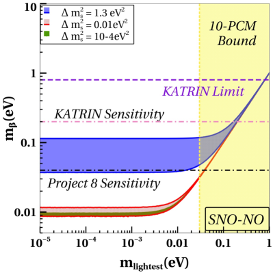
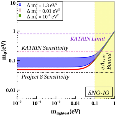
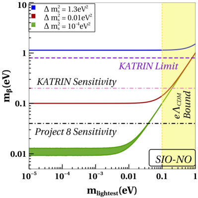
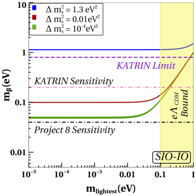
Figure 3: Kinematic mass $m_{\beta}$ from tritium $\beta$ decay in different scenarios of SNO-NO (top-left), SNO-IO (top-right), SIO-NO (bottom-left), and SIO-IO (bottom-right) for $\Delta m_{s}^{2}=10^{-4}\,\rm eV^{2}$ (green), $\Delta m_{s}^{2}=0.01\,\rm eV^{2}$ (red) and $\Delta m_{s}^{2}=1.3\,\rm eV^{2}$ (blue).

Table 4: 3$\sigma$ ranges of different combinations of oscillation parameters relevant to understanding kinematic mass ($m_{\beta}$) in the 3+1 scenario.

$|U_{e2}|^{2}\,\Delta m_{\rm sol}^{2}$	$(1-|U_{e2}|^{2})\,\Delta m_{\rm sol}^{2}$	$|U_{e3}|^{2}\,\Delta m_{\rm atm}^{2}$	$|U_{e4}|^{2}\,\Delta m_{s}^{2}$
$\times 10^{-5}$	$\times 10^{-5}$	$\times 10^{-5}$	$\Delta m_{s}^{2}=10^{-4}\,\rm eV^{2}$	$\Delta m_{s}^{2}=0.01\,\rm eV^{2}$	$\Delta m_{s}^{2}=1.3\,\rm eV^{2}$
$(1.77:2.65)$	$(4.57:5.95)$	$(4.86:6.24)$	$(1:2)\times 10^{-5}$	$(0.5:5)\times 10^{-5}$	$(0.13:1.3)\times 10^{-2}$

The following observations can be made from Fig. (3),

• KATRIN’s future sensitivity allows us to probe $m_{\beta}$ only above $m_{\rm lightest}\sim 0.2$ eV for SNO-NO, SNO-IO for all values of $\Delta m_{s}^{2}$. In case of SIO-NO, SIO-IO KATRIN will be able to probe the entire spectrum of $m_{\rm lightest}$ for $\Delta m_{s}^{2}=1.3$ eV², and above $m_{\rm lightest}\sim 0.02$ eV for $\Delta m_{s}^{2}=10^{-4},0.01$ eV².

• The sensitivity of Project 8 allows us to probe $m_{\beta}$ only above $m_{\rm lightest}\sim 0.03$ eV for SNO-NO and SIO-NO of $\Delta m_{s}^{2}=10^{-4}\,\rm eV^{2}$. However, Project 8 experiment can probe SNO-IO, SIO-NO, and SIO-IO for $\Delta m_{s}^{2}=0.01\,\rm eV^{2}$ and $1.3\,\rm eV^{2}$ in the entire range of $m_{\rm lightest}$.

• SNO-NO: Using Eqn. (8), $m_{\beta}$ can be approximated as

  $$m_{\beta}^{SNO-NO} = \sqrt{m_{\rm lightest}^{2}+|U_{e2}|^{2}\,\Delta m_{\rm sol}^{2}+|U_{e3}|^{2}\,\Delta m_{\rm atm}^{2}+|U_{e4}|^{2}\,\Delta m_{s}^{2}}$$ (17)

  • For $m_{\rm lightest}<\sqrt{\Delta m_{\rm sol}^{2}}<\sqrt{\Delta m_{\rm atm}^{2}}$ , it is seen from table (4) that the second, third and the fourth term in Eqn. (17) varies in the similar range for $\Delta m_{s}^{2}=10^{-4}\,\rm eV^{2}$ and $\Delta m_{s}^{2}=0.01\,\rm eV^{2}$. Hence $m_{\beta}^{SNO-NO}$ varies as $(0.009:0.01)$ and $(0.008:0.011)\,\rm eV$. In the case of $\Delta m_{s}^{2}=1.3\,\rm eV^{2}$, $m_{\beta}^{SNO-NO}\approx|U_{e4}|\,\sqrt{\Delta m_{s}^{2}}$ and varies between $(0.036:0.114)\,\rm eV$.

  • For $\sqrt{\Delta m_{\rm sol}^{2}}<m_{\rm lightest}<\sqrt{\Delta m_{\rm atm}^{2}}<\sqrt{\Delta m_{s}^{2}}$, $m_{\beta\beta}^{SNO-NO}\approx\,m_{\rm lightest}$ for $\Delta m_{s}^{2}=10^{-4}\,\rm eV^{2}$ and $\Delta m_{s}^{2}=0.01\,\rm eV^{2}$. Whereas $|U_{e4}|^{2}\,\Delta m_{s}^{2}$ still dominates in this region for $\Delta m_{s}^{2}=1.3\,\rm eV^{2}$.

  • For $\sqrt{\Delta m_{\rm atm}^{2}}<<|U_{e4}|\,\sqrt{\Delta m_{s}^{2}}<<m_{\rm lightest}$, $m_{\beta}^{SNO-NO}$ is completely determined by the value of $m_{\rm lightest}$.

• SNO-IO:

  $$m_{\beta}^{SNO-IO} \approx \sqrt{m_{\rm lightest}^{2}+\Delta m_{\rm atm}^{2}+|U_{e4}|^{2}\,\Delta m_{s}^{2}}$$ (18)

  • For $m_{\rm lightest}<<\Delta m_{\rm sol}^{2}<\Delta m_{\rm atm}^{2}$, $m_{\beta}^{SNO-IO}\approx\sqrt{\Delta m_{\rm atm}^{2}}\approx 0.05\,\rm eV$ for $\Delta m_{s}^{2}=10^{-4}\,\rm eV^{2}$ and $0.01\,\rm eV^{2}$ as $|U_{e4}|^{2}$ is very small. For $\Delta m_{s}^{2}=1.3\,\rm eV^{2}$, the value of $m_{\beta}^{SNO-IO}\approx\,\sqrt{\Delta m_{\rm atm}^{2}+|U_{e4}|^{2}\,\Delta m_{s}^{2}}$. Thus, the value of $m_{\beta}$ for $\Delta m_{s}^{2}=1.3\,\rm eV^{2}$ is greater than the $\sqrt{\Delta m_{\rm atm}^{2}}$ till $m_{2}\approx 0.1\,\rm eV$ .

  • $0.1<<m_{\rm lightest}$ , $m_{\beta}^{SNO-IO}\approx\,m_{\rm lightest}$ for the values of $\Delta m_{s}^{2}$. Hence, for higher $m_{\rm lightest}$, the behaviour of $m_{\beta}$ is fully characterised by $m_{\rm lightest}$.

• SIO-NO:

  $$m_{\beta}^{SIO-NO} = \sqrt{m_{\rm lightest}^{2}+\Delta m_{s}^{2}+|U_{e2}|^{2}\,\Delta m_{\rm sol}^{2}+|U_{e3}|^{2}\,\Delta m_{\rm atm}^{2}}$$ (19)

  • For $m_{\rm lightest}<<\sqrt{\Delta m_{\rm sol}^{2}}<<\sqrt{\Delta m_{\rm atm}^{2}}$, $m_{\beta}^{SIO-NO}\approx\sqrt{\Delta m_{s}^{2}}$ for $\Delta m_{s}^{2}=0.01\,\rm eV^{2}$ and $1.3\,\rm eV^{2}$. For $\Delta m_{s}^{2}=10^{-4}\,\rm eV^{2}$ , second and third term vary $\sim 10^{-5}$ , so we get a small variation due to that.

  • For $\sqrt{\Delta m_{s}^{2}}<<m_{\rm lightest}$, $m_{\beta}^{SIO-NO}\approx m_{\rm lightest}$, and the value value of $m_{\beta}^{SIO-NO}$ depend on $m_{\rm lightest}$ only.

• SIO-IO:

  • For $\Delta m_{s}^{2}>\Delta m_{\rm atm}^{2}$, $m_{\beta}^{SIO-IO}$ can be written as

    $$m_{\beta}^{SIO-IO} = \sqrt{m_{\rm lightest}^{2}+\,\Delta m_{s}^{2}}$$ (20)

    In this case, the conclusions are similar to SIO-NO for $\Delta m_{s}^{2}=0.01\,\rm eV^{2}$ and $1.3\,\rm eV^{2}$.

  • For $\Delta m_{s}^{2}<\Delta m_{\rm atm}^{2}$, $m_{\beta\beta}^{SIO-IO}$ can be expressed as

    $$m_{\beta}^{SIO-IO} = \sqrt{m_{\rm lightest}^{2}+\Delta m_{\rm atm}^{2}}$$ (21)

    In this case, for lower $m_{\rm lightest}\,(<\sqrt{\Delta m_{\rm atm}^{2})}$ region , $m_{\beta}^{SIO-IO}\approx\sqrt{\Delta m_{\rm atm}^{2}}\approx 0.05\,\rm eV$. For higher values of $m_{\rm lightest}\,(>\sqrt{\Delta m_{\rm atm}^{2}})$, the value of $m_{\beta}^{SNO-IO}$ is proportional to $m_{\rm lightest}$ which leads to a straight line behavior in the figures.

  The expressions of $m_{\beta}^{2}$ in various $m_{lightest}$ limits are tabulated in table (9) in the appendix.

III.3 Bound from neutrinoless double beta decay

The cosmological observations and the tritium decay measurements are sensitive to the absolute neutrino mass scale, not to the nature of the neutrinos, i.e., whether the neutrinos are Dirac or Majorana. The neutrinoless double beta decay ($0\nu\beta\beta$) process can provide both pieces of information. The $0\nu\beta\beta$ decay process constrains the half-life of the decaying isotope, which can be expressed as,

$$T_{1/2} = \frac{m_{e}^{2}}{G_{0\nu}\,\left|\mathcal{M}_{0\nu}\right|^{2}\,m_{{\beta\beta}}^{2}},$$ (22)

where $m_{e}$ is electron mass, $G_{0\nu}$ denotes the leptonic phase space and $\mathcal{M}_{0\nu}$ is the nuclear transition matrix element of the decay and $m_{\beta\beta}$ is the effective Majorana mass which can be expressed as

$$\mathbf{m}_{\beta\beta} = \sum_{i}U_{ei}^{2}\,m_{i}$$ (23)

where $i$ runs over the light neutrino species.

The current upper limits are $m_{\beta\beta}\leq(36-156)$ meV and $(79-180)$ meV as reported by the KamLAND-Zen and GERDA experiments respectively. But recently, it has been pointed out that the nuclear matrix element calculations should include a short-range contribution that originated from the hard-neutrino exchange mechanism described in Cirigliano:2018hja ; Cirigliano:2019vdj . Ref. Scholer:2023bnn showed that the inclusion of the short-range contribution tightens the limit on $m_{\beta\beta}$ as $m_{\beta\beta}\leq\,(25-68)$ meV for KamLAND-Zen.

III.3.1 Standard three flavor framework

In the standard three flavor framework Eqn. (23) can be expressed as

$$\mathbf{m}_{\beta\beta}^{\rm Std.} = m_{1}\,c_{12}^{2}\,c_{13}^{2}+m_{2}\,s_{12}^{2}\,c_{13}^{2}\,e^{i\alpha}+m_{3}\,s_{13}^{2}\,e^{i\beta}\$$ (24)

Unlike neutrino oscillation experiments, the effective Majorana mass is sensitive to the Majorana phases of the neutrinos. In addition, the effective Majorana mass is also sensitive to the mass orderings.

In Figures (4,5,6), grey and light brown regions display the effective mass governing $0\nu\beta\beta$ as a function of the lowest mass in the standard three-flavor framework for NO and IO respectively. In these figures, the oscillation parameters are varied over their $3\sigma$ ranges as tabulated in the table (1), and Majorana phases ($\alpha,\beta$) are varied between $(0\,:\,\pi)$.

Normal Ordering ($m_{1}<m_{2}<m_{3}$)

• For $m_{\rm lightest}(m_{1})<<\sqrt{\Delta m_{\rm sol}^{2}}<<\sqrt{\Delta m_{\rm atm}^{2}}$, $m_{2}\approx\sqrt{\Delta m_{\rm sol}^{2}}\approx 0.01\,\rm eV$ and $m_{3}\approx\sqrt{\Delta m_{\rm atm}^{2}}\approx 0.05\,\rm eV$. The effective Majorana mass can be approximated as

  $$\mathbf{m}^{\rm Std-NO}_{\beta\beta} = \sqrt{\Delta m_{\rm atm}^{2}}c_{13}^{2}\left(\sqrt{r}\,s_{12}^{2}\,e^{i\,\alpha}+t_{13}^{2}\,e^{i\beta}\right),$$ (25)

  where $r=\frac{\Delta m_{\rm sol}^{2}}{\Delta m_{\rm atm}^{2}}$. Complete cancellation is possible if $\sqrt{r}\,s_{12}^{2}=t_{13}^{2}$. In table (5), we enlist different combinations of parameters appearing in the expression of $\mathbf{m}^{\rm Std-NO}_{\beta\beta}$. As can be seen from the table (5), the maximum value of $t_{13}^{2}$ is much less than $\sqrt{r}\,s_{12}^{2}$, so complete cancellation is not possible in this region. For $\alpha=\beta=0$, we get the highest value of $\mathbf{m}^{\rm Std-NO}_{\beta\beta}$, while the lowest value is obtained for $\alpha=0\,,\,\beta=\pi$ or $\alpha=\pi\,,\,\beta=0$. In this region, the effective mass satisfies $0.001\,\rm eV\lesssim\left|\mathbf{m}^{\rm Std-NO}_{\beta\beta}\right|\lesssim 0.004\,\rm eV$.

• For $m_{\rm lightest}\approx\sqrt{\Delta m_{\rm sol}^{2}}$. Here, $\mathbf{m}^{\rm Std-NO}_{\beta\beta}$ can be expressed as

  $$\mathbf{m}^{\rm Std-NO}_{\beta\beta} = \sqrt{\Delta m_{\rm atm}^{2}}\,c_{13}^{2}\left(\sqrt{r}c_{12}^{2}+\sqrt{r}\,s_{12}^{2}\,e^{i\,\alpha}+t_{13}^{2}\,e^{i\,\beta}\right)$$ (26)

  The effective mass attains minimum value for $\alpha=\beta=\pi$ and complete cancellation occurs when $\sqrt{r}\,\cos 2\theta_{12}=t_{13}^{2}$ From table (5), it can be inferred that complete cancellation is not possible in this region, which is also observed in Figures (4,5,6).

• From Fig. (4), it can seen that the value of $m_{\beta\beta}$ is very small in a region $0.002\,\rm eV\,\lesssim m_{\rm lightest}\,\lesssim\,0.007\,\rm eV$. This region is commonly referred to as the cancellation region. As an example, considering the mixing parameters equal to their best fit values and $m_{\rm lightest}=0.005\,$eV, we get $m_{\beta\beta}\approx\,10^{-4}$ for the Majorana phases $\alpha=\beta=\pi$.

Inverted Ordering ($m_{3}<m_{1}<m_{2}$)

• In the limit $m_{3}\,\approx 0$, $m_{1}\approx m_{2}\approx\sqrt{\Delta m_{\rm atm}^{2}}$ and the effective mass can be expressed as,

  $$\mathbf{m}^{\rm Std-IO}_{\beta\beta} = \sqrt{\Delta m_{\rm atm}^{2}}\,c_{13}^{2}\left(c_{12}^{2}+s_{12}^{2}\,e^{i\,\alpha}\right)$$ (27)

  In this region, $\mathbf{m}^{\rm Std-IO}_{\beta\beta}$ is bounded from below and above by minimum and maximum values as,

  $$\left|\mathbf{m}^{\rm Std-IO}_{\beta\beta}\right|_{\rm min} = \sqrt{\Delta m_{\rm atm}^{2}}\,c_{13}^{2}\cos 2\theta_{12}=0.02\,\rm eV$$

  $$\left|\mathbf{m}^{\rm Std-IO}_{\beta\beta}\right|_{\rm max} = \sqrt{\Delta m_{\rm atm}^{2}}\,c_{13}^{2}=0.05\,\rm eV$$ (28)

These bounds are reflected also in Figures (4,5,6).

Quasi Degenerate Spectrum ($m_{1}\approx m_{2}\approx m_{3}\,\gtrsim 0.05\,\rm eV$)

The region where $m_{\rm lightest}\gtrsim\sqrt{\Delta m_{\rm atm}^{2}}\gtrsim 0.05$ eV (for both mass orderings) , $m_{1}\,,\,m_{2}\,,\,m_{3}$ are approximately equal. This region is called the quasi-degenerate region. Here the effective mass can be expressed as

$$\mathbf{m}_{\beta\beta}^{\rm QD} = m_{0}\,c_{13}^{2}\left(c_{12}^{2}+s_{12}^{2}\,e^{i\alpha}+t_{13}^{2}\,e^{i\,\beta}\right)$$ (29)

In this region, cancellation is not possible, as $t_{13}^{2}\approx 0.02,s_{12}^{2}\approx 0.3$ will not be able to cancel out $c_{12}^{2}\approx 0.7$ as can be seen from the Fig. (4,5,6). This region is in serious tension with the cosmological observations because, for three degenerate neutrinos, the bound on $m_{\rm lightest}\,<\,0.05$ eV considering $\sum m_{\nu}<0.16$ eV (from Eqn. (13)).

Table 5: 3$\sigma$ ranges of different combinations of oscillation parameters relevant to understanding the effective Majorana mass in the standard three-flavor scenario.

Param.	$\sqrt{r}$	$\sqrt{r}\,s_{12}^{2}$	$\sqrt{r}\,\cos 2\theta_{12}$	$t_{13}^{2}$	$\sqrt{r}\,t_{13}^{2}$
Max	0.18	0.0614	0.0828	0.0246	0.00443
Min	0.16	0.0432	0.0509	0.0204	0.00326

III.3.2 3+1 framework

In this subsection, the behavior of $m_{\beta\beta}$ is studied in the context of various mass ordering schemes in the presence of a light sterile neutrino. The plots in Figs. (4, 5, 6, 7) are generated by allowing all the oscillation parameters to vary in their $3\sigma$ range as mentioned in table 1, and the sterile parameters are varied according to the table (2).

$\star$ SNO-NO
The effective Majorana mass in this scenario can be written as

$$m_{\beta\beta}^{\rm SNO-NO} = c_{14}^{2}\,\left|\mathbf{m}^{\rm Std-NO}_{\beta\beta}+t^{2}_{14}\,m_{4}\,e^{i\,\gamma}\right|$$ (30)

where $\mathbf{m}^{\rm Std-NO}_{\beta\beta}$ is the standard three flavor effective mass for normal ordering. In Fig. (4), we have plotted $m_{\beta\beta}^{\rm SNO-NO}$ as a function of the lightest neutrino mass ($m_{\rm lightest}=m_{1}$) for the three mass squared differences. To explain the behavior of $m_{\beta\beta}^{\rm SNO-NO}$ in Fig. (4), we consider different limits of $m_{\rm lightest}$.

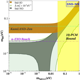
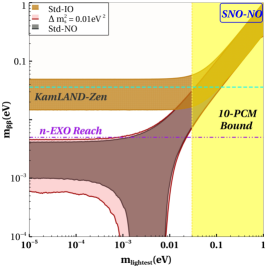
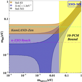
Figure 4: $m_{\beta\beta}$ is plotted for SNO-NO (green) scenario against the lightest neutrino mass with the mass squared difference ($\Delta m_{s}^{2}$) = $10^{-4}\rm eV^{2}$ (green), 0.01 $\rm eV^{2}$ (red), and 1.3 $\rm eV^{2}$(blue) along with standard three flavor NO (grey) and IO (brown) .

Table 6: 3$\sigma$ ranges of different combinations of oscillation parameters relevant to understanding the effective Majorana mass for SNO-NO in the 3+1 framework.

Regions	$\mathbf{m}^{\rm Std-NO}_{\beta\beta}$ (eV)	$\left|m_{4}\,t_{14}^{2}\right|$ (eV)
		$\Delta m_{s}^{2}\ =10^{-4}\,\rm eV^{2}$	$\Delta m_{s}^{2}\,=0.01\,\rm eV^{2}$	$\Delta m_{s}^{2}=1.3\,\rm eV^{2}$
$m_{1}\approx 0$	0.001 : 0.004	0.001 : 0.002	$5\times 10^{-5}:10^{-4}$	0.001 : 0.01
$m_{1}\approx\sqrt{\Delta m_{\rm sol}^{2}}$	0.0018 : 0.018	0.0014 : 0.003	$5\times 10^{-5}:10^{-4}$	0.001 : 0.01
$m_{1}\approx 0.1$	0.02 : 0.1	0.01 : 0.02	$5\times 10^{-4}:10^{-3}$	0.001 : 0.01

The values of different terms in Eqn. (30) are mentioned for various limits of $m_{1}$ in the table (6) where the maximum value of $m_{\beta\beta}^{\rm SNO-NO}$ corresponds to $\gamma=0$ and minimum is for $\gamma=\pi$. The important points are as follows:

• For $m_{1}<<\sqrt{\Delta m_{\rm sol}^{2}}<<\sqrt{\Delta m_{\rm atm}^{2}}<<\sqrt{\Delta m_{s}^{2}}$, it is seen from table (6) that for $\Delta m_{s}^{2}=10^{-4},1.3$ eV² complete cancellation is possible between $\mathbf{m}^{\rm Std-NO}_{\beta\beta}$ and $m_{4}\,t_{14}^{2}$ for $\gamma=\pi$.

• For $m_{1}\approx\sqrt{\Delta m_{\rm sol}^{2}}$, complete cancellations continue to occur for $\Delta m_{s}^{2}=10^{-4},1.3$ eV².

• At higher values of $m_{1}\approx 0.1$ eV, complete cancellation happens only for $\Delta m_{s}^{2}=10^{-4}$ eV² as seen from third row.

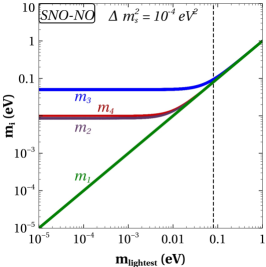
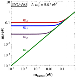
Figure 12: variation of masses with respect to the lightest neutrino mass for SNO-NO

• In the 3+1 scenario quasi-degenerate (QD) condition will arise when $m_{1}\approx m_{2}\approx m_{3}\approx m_{4}$. As seen in Fig.(12) (A), the QD region occurs around $0.08,0.2$ eV for $\Delta m_{s}^{2}=10^{-4},0.01$ eV². KamLAND-Zen and nEXO both can probe a fraction of the QD region for $\Delta m_{s}^{2}=10^{-4}$ eV² and the entire region for $\Delta m_{s}^{2}=0.01$ eV². However, cosmological bounds ($m_{1}>0.03$ eV) reject the QD region for both values of $\Delta m_{s}^{2}$.

$\star$ SNO-IO
Effective Majorana mass from double beta decay can be expressed as

$$m_{\beta\beta}^{\rm SNO-IO} = c_{14}^{2}\left|\mathbf{m}^{\rm Std-IO}_{\beta\beta}+t_{14}^{2}m_{4}\,e^{i\gamma}\right|$$ (31)

We have plotted $m_{\beta\beta}^{\rm SNO-IO}$ as a function of the lightest neutrino mass ($m_{3}$) for the three mass squared differences in the Fig. (5). The values of the terms in Eqn. (31) are enlisted in the table (7).

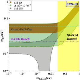
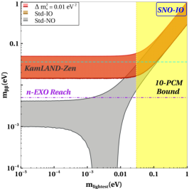
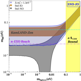
Figure 5: $m_{\beta\beta}$ is plotted for SNO-IO scenario against the lightest neutrino mass with the mass squared difference ($\Delta m_{s}^{2}$) = $10^{-4}\rm eV^{2}$ (green), 0.01 $\rm eV^{2}$ (red), 1.3 $\rm eV^{2}$ (blue) along with standard three flavor Normal Ordering (grey) and Inverted Ordering (brown) .

Table 7: The 3$\sigma$ ranges of different combinations of oscillation parameters relevant to understanding the effective Majorana mass for SNO-IO in the 3+1 framework.

Regions	$\mathbf{m}^{\rm Std-IO}_{\beta\beta}$ (eV)	$m_{4}\,t_{14}^{2}$ (eV)
		$\Delta m_{s}^{2}\ =10^{-4}\,\rm eV^{2}$	$\Delta m_{s}^{2}\,=0.01\,\rm eV^{2}$	$\Delta m_{s}^{2}=1.3\,\rm eV^{2}$
$m_{3}\approx 0$	$0.02\,:\,0.05$	$0.005\,:\,0.01$	$5\times 10^{-5}\,:\,5\times 10^{-4}$	$0.001\,:\,0.01$
$m_{3}\approx 0.1$	$0.03\,:\,0.1$	$0.01\,:\,0.025$	$7.5\times 10^{-5}\,:\,7.5\times 10^{-4}$	$0.001\,:\,0.01$

The notable points in the SNO-IO case are as follows,

• It is evident from table (7), that the minimum value of $\mathbf{m}^{\rm Std-IO}_{\beta\beta}$ is always greater than the maximum value of $m_{4}\,t_{14}^{2}$ for all the three mass squared differences. Hence, complete cancellation is not possible for the entire range of $m_{\rm lightest}.$

• The value of $m_{4}\,t_{14}^{2}$ for $\Delta m_{s}^{2}=0.01\,\rm eV^{2}$ is very small compared to $\mathbf{m}^{\rm Std-IO}_{\beta\beta}$. Therefore, $m_{\beta\beta}^{\rm SNO-IO}$ is approximately equal to $\mathbf{m}^{\rm Std-IO}_{\beta\beta}$ which is visible from the middle panel of Fig. (5).

• For $\Delta m_{s}^{2}=10^{-4}\,\rm eV^{2}$ and $1.3\,\rm eV^{2}$, the minimum value of $m_{\beta\beta}^{\rm SNO-IO}\approx 0.01\,\rm eV$ is attained for $\gamma=\pi$ which can be probed partially in the future experiment, nEXO.

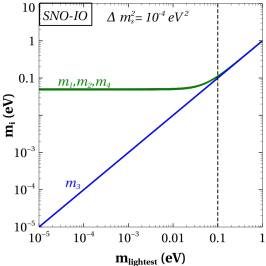
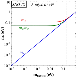
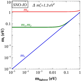
Figure 13: variation of masses with respect to the lightest neutrino mass for SNO-IO

• The QD regions, as observed from Fig. (13), is occurred at $m_{3}>0.1,0.2$ eV for $\Delta m_{s}^{2}=10^{-4},\,0.01$ eV² respectively. Although the QD region is disfavored by cosmology for both the $\Delta m_{s}^{2}$ values, KamLAND-Zen and nEXO can probe this region partially for $\Delta m_{s}^{2}=10^{-4}$ eV² and completely for $\Delta m_{s}^{2}=0.01$ eV².

$\star$ SIO-NO
The effective Majorana mass is expressed as,

$$m^{\rm SIO-NO}_{\beta\beta} \approx c_{14}^{2}\left(\sqrt{m_{4}^{2}+\Delta m_{s}^{2}}\left(c_{12}^{2}+s_{12}^{2}\,e^{i\alpha}\right)+m_{4}\,t_{14}^{2}\,e^{i\,\gamma}\right)\hskip 30.00005pt\left[\Delta m_{s}^{2}>\Delta m_{\rm atm}^{2}\right]$$

$$m^{\rm SIO-NO}_{\beta\beta} \approx c_{14}^{2}\,\left(c_{13}^{2}\left(\sqrt{m_{4}^{2}+\Delta m_{s}^{2}}\left(c_{12}^{2}+s_{12}^{2}\,e^{i\alpha}\right)+\sqrt{m_{4}^{2}+\Delta m_{\rm atm}^{2}}\,s_{13}^{2}\,e^{i\beta}\right)+m_{4}\,t_{14}^{2}\,e^{i\,\gamma}\right)$$ (32)

$$\hskip 250.00038pt\left[\Delta m_{s}^{2}<\Delta m_{\rm atm}^{2}\right]$$

Here, we have used the mass relations mentioned in Eqn. (10). In Fig. (6), we have shown $m_{\beta\beta}$ as function of $m_{\rm lightest}$ ($m_{4}$) in three panels corresponding to different values of $\Delta m_{s}^{2}$. The table (8) depicts the terms of Eqn. (III.3.2).

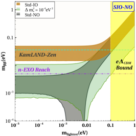
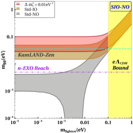
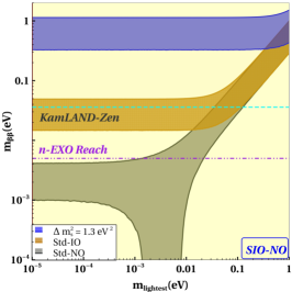
Figure 6: $m_{\beta\beta}$ is plotted for SIO-NO (green) scenario against the lightest neutrino mass with the mass squared difference ($\Delta m_{s}^{2}$) = ($10^{-4}\rm\,eV^{2}$, 0.01 $\rm eV^{2}$, 1.3 $\rm eV^{2}$) along with standard three flavor Normal Ordering (red) and Inverted Ordering (yellow) .

Table 8: The 3$\sigma$ ranges of different combinations of oscillation parameters relevant to understanding the effective Majorana mass for SIO-NO in the 3+1 framework.

Regions	$\sqrt{\Delta m_{s}^{2}}\,\cos 2\theta_{12}$ (eV)			$\sqrt{\Delta m_{\rm atm}^{2}}\,t_{13}^{2}$ (eV)	$m_{4}\,t_{14}^{2}$ (eV)
	$\Delta=10^{-4}$	$\Delta=0.01$	$\Delta=1.3$		$\Delta=10^{-4}$	$\Delta=0.01$	$\Delta=1.3$
$m_{4}\approx 0$	$0.003$	0.03	0.33	0.001	0	0	0
$m_{4}\approx 0.01$	$0.003$	0.03	0.33	0.001	0.001 : 0.002	$5.\,10^{-5}:5.\,10^{-4}$	$10^{-5}:10^{-4}$

• For the region where the lightest mass is negligible, Eqn. (10) will be,

  $$m_{4}\approx 0,\quad m_{2} \approx \,m_{1}\,\approx m_{3}\,\approx\sqrt{\Delta m_{s}^{2}}\hskip 60.00009pt\left(\Delta m_{s}^{2}>\Delta m_{\rm atm}^{2}\right)$$

  $$m_{4}\approx 0,\quad m_{1} \approx m_{2}\approx\,\sqrt{\Delta m_{s}^{2}},\,\,m_{3}\,\approx\sqrt{\Delta m_{\rm atm}^{2}}\hskip 10.00002pt\left(\Delta m_{s}^{2}<\Delta m_{\rm atm}^{2}\right)$$ (33)

  Effective Majorana mass from double beta decay

  $$m^{\rm SIO-NO}_{\beta\beta} = \sqrt{\Delta m_{s}^{2}}\left(c_{12}^{2}+s_{12}^{2}\,e^{i\alpha}\right)\hskip 130.0002pt\left(\Delta m_{s}^{2}>\Delta m_{\rm atm}^{2}\right)$$

  $$m^{\rm SIO-NO}_{\beta\beta} = c_{13}^{2}\,c_{14}^{2}\left(\sqrt{\Delta m_{s}^{2}}\left(c_{12}^{2}+s_{12}^{2}\,e^{i\alpha}\right)+\sqrt{\Delta m_{\rm atm}^{2}}\,t_{13}^{2}\,e^{i\beta}\right)\hskip 10.00002pt\left(\Delta m_{s}^{2}<\Delta m_{\rm atm}^{2}\right)$$

  In the first case, complete cancellation can happen for $\alpha=\pi$ and $c_{12}^{2}=s^{2}_{12}$. But, since $\theta_{12}$ is less than $45^{\circ}$, this cannot happen, as shown in Fig. (6) for $\Delta m_{s}=10^{-4}$ eV². In the second case, complete cancellation occurs for $\alpha=\beta=\pi$ and

  $$\sqrt{\Delta m_{s}^{2}}\,\cos 2\theta_{12}=\sqrt{\Delta m_{\rm atm}^{2}}\,t_{13}^{2}$$ (35)

  This condition is not satisfied for $\Delta m_{s}^{2}=1.3,\,0.01$ eV² as can be seen from table (1) and table (8). The value of $m_{\beta\beta}^{\rm SIO-NO}$ varies between $(0.3\,:\,1)$ eV and $(0.001\,:0.01\,)$ eV for $\Delta m_{s}^{2}=1.3,10^{-4}$ eV² respectively, as seen in from Fig. (6).

• Around $m_{4}\approx 0.01\,$eV, in case of $\Delta m_{s}^{2}=0.01\,\rm eV^{2}\,and\,1.3\,eV^{2}$, the sterile contribution is negligible compared to other terms as the value of $\theta_{14}$ is small and thus no cancellation occurs. But due to large $\theta_{14}$ for $\Delta m_{s}^{2}=10^{-4}$, the value of $m_{4}\,t_{14}^{2}$ varies between $(0.001\,:\,0.002)$ which allows us to have a narrow cancellation region for $\alpha=\beta=\gamma=\pi$.

• It is to be noted that the KamLAND-ZEN experiment disallows the entire parameter space of $m_{\beta\beta}^{\rm SIO-NO}$ for $\Delta m_{s}^{2}=1.3\rm\,eV^{2}$. For $\Delta m_{s}^{2}=0.01$ eV² a part of the parameter space gets disfavored for all values of $m_{\rm lightest}$, whereas for $\Delta m_{s}^{2}=10^{-4}$ eV² regions with higher values of $m_{\rm lightest}(>0.3\,\rm eV)$ are disfavored. For $10^{-4}$ eV², the allowed region of $m_{\beta\beta}^{\rm SIO-NO}$ can be partially probed by nEXO experiment.

$\star$ SIO-IO

In three panels of Fig. (7), Majorana mass $m_{\beta\beta}$ in SIO-IO scenario has been plotted against $m_{\rm lightest}=m_{4}$.

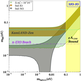
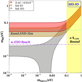
Figure 7: $m_{\beta\beta}$ is plotted for SIO-IO (green) scenario against the lightest neutrino mass with the mass squared difference ($\Delta m_{s}^{2}$) = ($10^{-4}\rm\,eV^{2}$, 0.01 $\rm eV^{2}$, 1.3 $\rm eV^{2}$) along with standard three flavor Normal Ordering (red) and Inverted Ordering (yellow) .

• For $\Delta m_{s}^{2}>\Delta m_{\rm atm}^{2}$, $m_{\beta\beta}$ is exactly similar to the SIO-NO scenario ($\Delta m_{s}^{2}>\Delta m_{\rm atm}^{2}$). Thus, the results and the conclusions remain identical.

• For $\Delta m_{s}^{2}<\Delta m_{\rm atm}^{2}$ , the value of $m_{\beta\beta}$ in a region where $m_{\rm lightest}$ is small, can be approximated as

  $$\left(m_{\beta\beta}^{\rm SIO-IO}\right)_{\Delta m_{s}^{2}<\Delta m_{\rm atm}^{2}}=\sqrt{\Delta m_{\rm atm}^{2}}\,c_{14}^{2}\left(c_{12}^{2}+s_{12}^{2}\,e^{i\alpha}+t_{14}^{2}\,e^{i\gamma}\right)$$ (36)

  Here, complete cancellation requires $\alpha=\gamma=\pi$ and

  $$\cos 2\theta_{12}=t_{14}^{2}$$ (37)

  In this region, complete cancellation is not possible as Eqn. (37) is not satisfied for the allowed range of mixing angle $\theta_{14}$ given in table (2).

• When $m_{\rm lightest}>\sqrt{\Delta m_{\rm atm}^{2}}$ , $m_{1}\approx m_{2}\approx m_{3}\approx m_{4}\approx m_{0}$ and the value of $m_{\beta\beta}$ can be written as

  $$\left(m_{\beta\beta}^{\rm SIO-IO}\right)_{\Delta m_{s}^{2}<\Delta m_{\rm atm}^{2}}=m_{0}\,c_{14}^{2}\left(c_{12}^{2}+s_{12}^{2}\,e^{i\alpha}+t_{14}^{2}\,e^{i\gamma}\right)$$ (38)

  In this region, cancellation is also not possible, and $m_{\beta\beta}$ is proportional to the value of the lightest mass.

• It can be seen from Fig. (7), higher values of $m_{\beta\beta}$ are disfavored by KamLAND-Zen for all values of $m_{\rm lightest}$ and nEXO can rule out an even greater part of the parameter space in the absence of any signal.

The expressions of $m_{\beta\beta}$ in various $m_{lightest}$ limits are tabulated in table (10) in the appendix.

III.4 Correlations

As discussed, cosmology, direct mass measurement experiment (single $\beta$ decay), and $0\nu\beta\beta$ decay put independent constraints on the absolute mass scale of the neutrino. In this section, we discuss the correlations of the mass observable amongst each other. We have plotted in Figs. (8-11), the correlation of $m_{\beta}$ against $\Sigma$ (left), $m_{\beta\beta}$ against $\Sigma$ (middle), and $m_{\beta\beta}$ against $m_{\beta}$ (right) for all the mass spectra. The yellow-shaded and the brown-hatched regions correspond to cosmologically excluded regions mentioned in Eqn. (13) and Eqn. (14), respectively. The other horizontal and vertical lines are the current experimental limits (KamLAND-Zen [Cyan]) and future sensitivity (KATRIN [Pink], Project 8 [Black], nEXO [Magenta]) with their respective color mention in brackets. Blue, red, and green regions in the plots of Fig. (8-11) correspond to $\Delta m_{s}^{2}=1.3,\,0.01,\,10^{-4}$ eV² respectively.

1. SNO-NO:

   

   

   

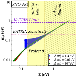
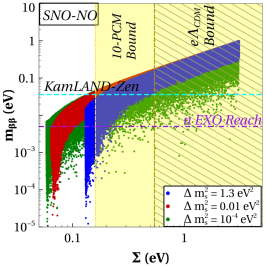
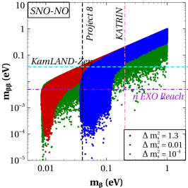
   Figure 8: Correlations of $m_{\beta}$ against and $\Sigma$(left) , $m_{\beta\beta}$ against $\Sigma$ (middle) and $m_{\beta\beta}$ against $m_{\beta}$ (right) for SNO-NO is plotted here. The green, blue, and red regions describe the values for $\Delta m_{s}^{2}=10^{-4}\rm\,eV^{2}$, $0.01\rm\,eV^{2}$ and $1.3\rm\,eV^{2}$ respectively. The yellow-shaded and brown-hatched regions correspond to the exclusion regions by Eqn. (13) and Eqn. (14) respectively.

   The correlation plots for SNO-NO are shown in Fig. (8).

   • From the left panel, it is seen that the cosmological mass bound disfavors a large parameter space for all three mass-squared differences. The allowed region from cosmology will not be sensitive to KATRIN’s projected limit, but the proposed Project 8 experiment can probe the parameter space for $\Delta m_{s}^{2}=1.3\,\rm eV^{2}$.

   • From the middle panel, it is observed that some part of the parameter space disfavored by the cosmological bound is also disfavored by KamLAND-Zen. In the region allowed by cosmology, $m_{\beta}$ can be very low. Therefore, KamLAND-Zen can probe a very small part of it, and the projected sensitivity nEXO experiment can only probe some parts of these regions for all the mass-squared differences.

   • From the right panel, it can be noted that the proposed experiments nEXO and Project-8 together can rule out almost the entire parameter space for $\Delta m_{s}^{2}=1.3$ eV² in the absence of any signal. However, in the case of $\Delta m_{s}^{2}=0.01,10^{-4}$ eV², only parts of the parameter space can be probed by the upcoming above-cited experiments.

2. SNO-IO:

   

   

   

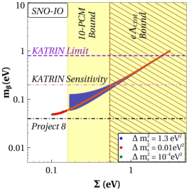
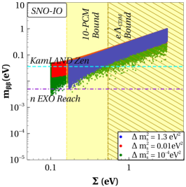
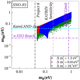
   Figure 9: Correlations of $m_{\beta}$ against and $\Sigma$(left) , $m_{\beta\beta}$ against $\Sigma$ (middle) and $m_{\beta\beta}$ against $m_{\beta}$ (right) for SNO-IO is plotted here. The green, blue, and red regions describe the values for $\Delta m_{s}^{2}=10^{-4}\rm\,eV^{2}$, $0.01\rm\,eV^{2}$ and $1.3\rm\,eV^{2}$ respectively. The yellow-shaded and brown-hatched regions correspond to the exclusion regions by Eqn. (13) and Eqn. (14) respectively.

   Fig. (9) shows the correlation plots for SNO-IO.

   • From the left panel, it is visible that $\Delta m_{s}^{2}=1.3\,\rm eV^{2}$ is ruled out by stringent cosmological limit. But for $\Delta m_{s}^{2}\,=10^{-4}\,\rm eV^{2}$ and $0.01\,\rm eV^{2}$ small parts of parameter space are allowed by cosmology and KATRIN’s projected sensitivity. These allowed regions can be completely probed in the proposed Project 8 experiment.

   • It can be noted from the middle panel that KamLAND-Zen and cosmology rule out a large part of the parameter space for all the mass-squared differences. For $\Delta m_{s}^{2}=0.01,\,10^{-4}\,\rm eV^{2}$, the region allowed by cosmology and KamLAND-Zen can be probed in future experiment nEXO.

   • From the right panel, it is observed that Project 8 and nEXO experiments together can probe the entire parameter space for $\Delta m_{s}^{2}=\,10^{-4},\,0.01$ and $1.3\,\rm eV^{2}$.

3. SIO-NO:

   

   

   

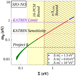
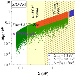
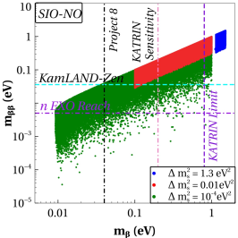
   Figure 10: Correlations of $m_{\beta}$ against and $\Sigma$(left) , $m_{\beta\beta}$ against $\Sigma$ (middle) and $m_{\beta\beta}$ against $m_{\beta}$ (right) for SNO-IO is plotted here. The green, blue, and red regions describe the values for $\Delta m_{s}^{2}=10^{-4}\rm\,eV^{2}$, $0.01\rm\,eV^{2}$ and $1.3\rm\,eV^{2}$ respectively. The yellow-shaded and brown-hatched regions correspond to the exclusion regions by Eqn. (13) and Eqn. (14) respectively.

   In Fig. (10), correlations between the mass variables for the SIO-NO scenario are plotted.

   • The left and middle panels show that $e\Lambda_{CDM}$ model only allows a part of the parameter space for $\Delta m_{s}^{2}=0.01,10^{-4}$ eV², however with the cosmological bound only $\Delta m_{s}^{2}=10^{-4}\,\rm eV^{2}$ is preferred.

   • From the left panel, it is visible that the current KATRIN bound can’t probe the regions allowed by cosmological and $e\Lambda_{CDM}$ model. Only proposed Project 8 can probe allowed regions for $1.3\,\rm eV^{2}$.

   • The middle panel depicts that the KamLAND-Zen sensitivity will be able to probe the $e\Lambda_{CDM}$ favored regions of $10^{-4}\,\rm eV^{2}$ and $0.01\,\rm eV^{2}$ partially. The nEXO can completely probe allowed regions of $0.01\,\rm eV^{2}$.

   • It is to be noted from the right panel that the future experiments nEXO and Project 8 can together probe the entirety of the parameter space for $\Delta m_{s}^{2}=1.3,\,0.01$ eV², and a fraction of the regions for $\Delta m_{s}^{2}=10^{-4}$ eV².

4. SIO-IO:

   

   

   

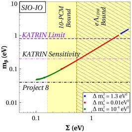
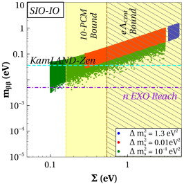
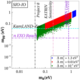
   Figure 11: Correlations of $m_{\beta}$ against and $\Sigma$(left) , $m_{\beta\beta}$ against $\Sigma$ (middle) and $m_{\beta\beta}$ against $m_{\beta}$ (right) is plotted here. The green, blue, black, and red regions describe SNO-NO, SNO-IO, SIO-NO & SIO-IO, respectively. The shaded regions correspond to the exclusion regions of the respective x-axis labels.

   The correlations amongst the mass variables for the SIO-IO scenario are plotted in Fig. (11).

   • From the left panel, we understand that the SIO-IO scenario is similar to the SIO-NO scenario. The only difference is that Project 8 will be able to probe the entire cosmologically allowed regions of $\Delta m_{s}^{2}=10^{-4}$ eV².

   • The middle panel portrays similar observations to that of SIO-NO apart from the fact that now future experiment nEXO can cover almost the total parameter space for all $\Delta m_{s}^{2}$ values considered by us.

   • From the right panel, it can be seen that the proposed experiments Project 8 and nEXO can together cover the entire parameter space for all the values of $\Delta m_{s}^{2}$.

IV Summary and Discussion

The results from short baseline neutrino oscillation experiments e.g. LSND and MiniBooNE and radio-chemical experiments e.g GALLEX, SAGE, & BEST indicate the possibility of having an extra neutrino state with $\mathcal{O}(\,\rm eV)$ mass squared difference. Moreover, the tension between the results of T2K and NO$\nu$A experiments can be improved by invoking an additional state mass squared difference $\sim 10^{-2}\,\rm eV^{2}$ and lack of upturn events in the solar neutrino spectra below 8 MeV can be explained by an ultralight sterile neutrino. Thus, sterile neutrinos with a very wide range of mass differences ($\Delta m_{s}^{2}=m_{4}^{2}-m_{1}^{2}$) have been proposed in the literature. The addition of a sterile state implies four mass spectra, namely: SNO-NO ($\Delta m_{s}^{2}>0\,,\,\Delta m_{\rm atm}^{2}>0$), SNO-IO ($\Delta m_{s}^{2}>0\,,\,\Delta m_{\rm atm}^{2}<0$), SIO-NO ($\Delta m_{s}^{2}<0\,,\,\Delta m_{\rm atm}^{2}>0$), and SIO-IO ($\Delta m_{s}^{2}<0\,,\,\Delta m_{\rm atm}^{2}<0$) where NO (IO) stands for +ve (-ve) value of $\Delta m^{2}_{31}$ and SNO(SIO) stand for +ve (-ve) value of $\Delta m^{2}_{41}$. The mass spectra are depicted in Fig. (1). We explore the implications of the mass spectra for sum of light neutrino masses from cosmology, beta decay, and $0\nu\beta\beta$ decay.

• The scenario of $\Delta m_{s}^{2}=1.3\,\rm eV^{2}$ with $\Delta m_{s}^{2}<0$ is known to be in conflict with the cosmological bound on the sum of neutrino masses. The specific bounds depend on the chosen data sets and the cosmological models used for fitting. Here we consider two different cosmological models: a 10 parameter cosmological model (10-PCM) and a 12 parameter cosmological model $(e\Lambda_{CDM})$ which provide the limit on the total mass of the light neutrino species as $\sum<0.16\,\rm eV$ and $\sum<0.52\,\rm eV$ respectively. We find that SIO-NO and SIO-IO is completely ruled out by cosmology. Moreover, such scenarios are disfavored from the current limit on $m_{\beta}$ by KATRIN experiment and also from the upper limit on $m_{\beta\beta}$ by KamLAND-Zen experiment. We want to emphasize that SIO-NO and SIO-IO scenarios for $\Delta m_{s}^{2}=1.3\,\rm eV^{2}$ are not only disfavored by cosmology but also by KATRIN and KamLAND-Zen. However, we see that SNO-NO and SNO-IO for $\Delta m_{s}^{2}=1.3\,\rm eV^{2}$ is still allowed below $m_{\rm lightest}\approx 0.1\,\rm eV$, in the limit of $e\Lambda_{CDM}$ model, KATRIN and KamLAND-Zen but proposed experiment Project 8 will be able to probe the scenarios with the projected limit of $m_{\beta}$.

• It is often believed that sterile neutrinos with mass-squared difference smaller than 1.3 $\rm eV^{2}$ can be allowed by cosmology. Here we find that, for $\Delta m_{s}^{2}=0.01\,\rm eV^{2}$, all mass spectra are allowed in $e\Lambda_{CDM}$ model up to a value of $m_{\rm lightest}\approx 0.1\,\rm eV$ but SIO-NO and SIO-IO is disfavored when 10-PCM model is considered whereas SNO-NO and SNO-IO scenarios remain valid up to $m_{\rm lightest}\sim 0.03\,\rm eV$. It is also noted that projected sensitivity from KATRIN experiments will not be able to probe the mass spectra, but SNO-IO, SIO-NO, and SIO-IO scenarios can be probed completely with Project 8’s proposed sensitivity. In the case of neutrinoless double decay measurements, KamLAND-Zen experiment ruled out most of the parameter space of SIO-NO and SIO-IO scenario for $\Delta m_{s}^{2}=0.01\,\rm eV^{2}$ and next generation experiment $nEXO$ will be able to probe the parameter space completely. Moreover, nEXO will also be able to probe the SNO-IO scenario completely for $\Delta m_{s}^{2}=0.01\,\rm eV^{2}$.

• It is seen from Fig. (2) that $\Delta m_{s}^{2}=10^{-4}\,\rm eV^{2}$ i.e sterile neutrino with very small mass-squared difference is allowed up to $m_{\rm lightest}\approx 0.03\,\rm eV$ and up to $m_{\rm lightest}\approx 0.1\,\rm eV$ from $e\Lambda_{CDM}$ model. In case of direct mass measurement, KATRIN’s projected limit can probe the mass spectra up to $m_{\rm lightest}\approx\,0.2\,\rm eV$ whereas Project 8 will be able to probe SNO-IO, SIO-IO scenarios completely and SNO-NO, SIO-NO scenarios up to $m_{\rm lightest}\approx 0.04\,\rm eV$. We also find that neither KamLAND-Zen nor nEXO can completely probe the mass spectra, but they rule out some parameter space for SNO-IO, SIO-NO and SIO-IO scenarios.

In conclusion, in the presence of a light sterile state, mass-related observables can provide constraints on the possible spectra and can disfavor some of these depending on the mass of the sterile state.

Appendix A Mass-spectrum

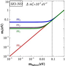
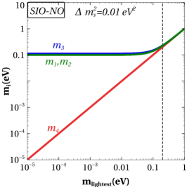
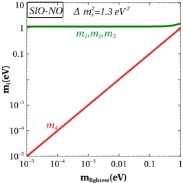
Figure 14: variation of masses with respect to the lightest neutrino mass for SIO-NO

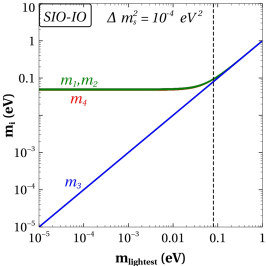
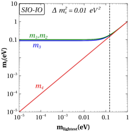
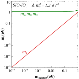
Figure 15: variation of masses with respect to the lightest neutrino mass for SIO-IO

Mass Spectra	Region	Expression of $m_{\beta}^{2}$
		(I) $\Delta m_{s}^{2}=10^{-4}\,\rm eV^{2}$	(II) $\Delta m_{s}^{2}=10^{-2}\,\rm eV^{2}$	(III) $\Delta m_{s}^{2}=1.3\,\rm eV^{2}$
SNO-NO	$m_{\rm lightest}<<\sqrt{\Delta m_{\rm sol}^{2}}<<\sqrt{\Delta m_{\rm atm}^{2}}$	$\Delta m_{\rm sol}^{2}|U_{e2}|^{2}+\Delta m_{\rm atm}^{2}|U_{e3}|^{2}+\Delta m_{s}^{2}|U_{e4}|^{2}$	same as (I)	$\Delta m_{s}^{2}|U_{e4}|^{2}$
	$\sqrt{\Delta m_{\rm sol}^{2}}<<m_{\rm lightest}<<\sqrt{\Delta m_{\rm atm}^{2}}$	$m_{\rm lightest}^{2}$.	same as (I)	$\Delta m_{s}^{2}|U_{e4}|^{2}$
SNO-IO	$m_{\rm lightest}<<\sqrt{\Delta m_{\rm sol}^{2}}<<\sqrt{\Delta m_{\rm atm}^{2}}$	$\Delta m_{\rm atm}^{2}$	$\Delta m_{\rm atm}^{2}$	$\Delta m_{\rm atm}^{2}+\Delta m_{s}^{2}\,|U_{e4}|^{2}$
	$\sqrt{\Delta m_{\rm atm}^{2}}\lesssim m_{\rm lightest}$	$m_{\rm lightest}^{2}$	$m_{\rm lightest}^{2}$	$m_{\rm lightest}^{2}+\Delta m_{s}^{2}\,|U_{e4}|^{2}$
	$\sqrt{\Delta m_{\rm atm}^{2}}<<m_{\rm lightest}$	$m_{\rm lightest}^{2}$	$m_{\rm lightest}^{2}$	$m_{3}^{2}$
SIO-NO	$m_{\rm lightest}<<\sqrt{\Delta m_{\rm sol}^{2}}<<\Delta m_{s}^{2}$	$\Delta m_{s}^{2}$	$\Delta m_{s}^{2}$	$\Delta m_{s}^{2}$
	$\sqrt{\Delta m_{s}^{2}}<<m_{\rm lightest}$	$m_{\rm lightest}^{2}$	$m_{\rm lightest}^{2}$	$m_{\rm lightest^{2}}$
SIO-IO	$m_{\rm lightest}<<\sqrt{\Delta m_{\rm atm}^{2}}$	same as SNO-IO	same as SIO-NO	same as SIO-NO
	$m_{s}^{2}<<\sqrt{\Delta m_{\rm atm}^{2}}<<m_{\rm lightest}$	$m_{\rm lightest}^{2}$	N.A	N.A.
	$\sqrt{\Delta m_{\rm atm}^{2}}<<m_{s}^{2}<<m_{\rm lightest}$	N.A.	$m_{\rm lightest}$	$m_{\rm lightest}$

Table 9: The table depicts expressions of $m_{\beta}^{2}$ in third, fourth, and fifth columns corresponding to $\Delta m_{s}^{2}=10^{-4},\,10^{-2},\,1.3\,\rm eV^{2}$ respectively for various mass spectra given in the first column under different regions shown in column two.

Mass Spectra	Region	Expression of $m_{\beta\beta}$
		(I) $\Delta m_{s}^{2}=10^{-4}\,\rm eV^{2}$	(II) $\Delta m_{s}^{2}=10^{-2}\,\rm eV^{2}$	(III) $\Delta m_{s}^{2}=1.3\,\rm eV^{2}$
SNO-NO	$m_{1}\approx 0$	$\sqrt{\Delta m_{\rm sol}^{2}}U_{e2}^{2}e^{i\alpha}+\sqrt{\Delta m_{\rm atm}^{2}}U_{e3}^{2}e^{i\beta}+\sqrt{\Delta m_{s}^{2}}U_{e4}^{1}e^{i\gamma}$	$\sqrt{\Delta m_{\rm sol}^{2}}U_{e2}^{2}e^{i\alpha}+\sqrt{\Delta m_{\rm atm}^{2}}U_{e3}^{2}e^{i\beta}$	same as (I)
	$m_{1}\approx m_{2}\approx m_{3}$	N.A.	$m_{1}\left[U_{e1}^{2}+U_{e2}^{2}e^{i\alpha}\right]$	same as (II)
	$m_{1}\approx m_{2}\approx m_{4}$	$m_{1}\left[U_{e1}^{2}+U_{e2}^{2}e^{i\alpha}+U_{e4}^{2}e^{i\gamma}\right]$	N.A.	N.A.
	$m_{1}\approx m_{2}\approx m_{3}\approx m_{4}$	$m_{1}\left[U_{e1}^{2}+U_{e2}^{2}e^{i\alpha}+U_{e4}^{2}e^{i\gamma}\right]$	$m_{1}\left[U_{e1}^{2}+U_{e2}^{2}e^{i\alpha}\right]$	N.A.
SNO-IO	$m_{3}\approx 0$	$\sqrt{\Delta m_{\rm atm}^{2}}\left[U_{e1}^{2}+U_{e2}^{2}e^{i\alpha}+U_{e4}^{2}e^{i\gamma}\right]$	$\sqrt{\Delta m_{\rm atm}^{2}}\left[U_{e1}^{2}+U_{e2}^{2}e^{i\alpha}\right]$	$\sqrt{\Delta m_{\rm atm}^{2}}\left[U_{e1}^{2}+U_{e2}^{2}e^{i\alpha}\right]+\sqrt{\Delta m_{s}^{2}}U_{e4}^{2}e^{i\gamma}$
	$m_{1}\approx m_{2}\approx m_{3}$	$m_{3}\left[U_{e1}^{2}+U_{e2}^{2}e^{i\alpha}+U_{e4}^{2}e^{i\gamma}\right]$	$m_{3}\left[U_{e1}^{2}+U_{e2}^{2}e^{i\alpha}\right]$	same as (II)
	$m_{1}\approx m_{2}\approx m_{3}\approx m_{4}$	$m_{3}\left[U_{e1}^{2}+U_{e2}^{2}e^{i\alpha}+U_{e4}^{2}e^{i\gamma}\right]$	$m_{3}\left[U_{e1}^{2}+U_{e2}^{2}e^{i\alpha}\right]$	N.A.
SIO-NO	$m_{4}\approx 0$	$\sqrt{\Delta m_{s}^{2}}\left[U_{e1}^{2}+U_{e2}^{2}e^{i\alpha}\right]+\sqrt{\Delta m_{\rm atm}^{2}}U_{e3}^{2}e^{i\beta}$	$\sqrt{\Delta m_{s}^{2}}\left[U_{e1}^{2}+U_{e2}^{2}e^{i\alpha}\right]$	same as (II)
	$m_{1}\approx m_{2}\approx m_{4}$	$m_{4}\left[U_{e1}^{2}+U_{e2}^{2}e^{i\alpha}+U_{e4}^{2}e^{i\gamma}\right]$	$m_{4}\left[U_{e1}^{2}+U_{e2}^{2}e^{i\alpha}\right]$	N.A.
	$m_{1}\approx m_{2}\approx m_{3}\approx m_{4}$	$m_{4}\left[U_{e1}^{2}+U_{e2}^{2}e^{i\alpha}+U_{e4}^{2}e^{i\gamma}\right]$	$m_{4}\left[U_{e1}^{2}+U_{e2}^{2}e^{i\alpha}\right]$	N.A.
SIO-IO	$m_{\rm lightest}\approx 0$	$\sqrt{\Delta m_{\rm atm}^{2}}\left[U_{e1}^{2}+U_{e2}^{2}e^{i\alpha}+U_{e4}^{2}e^{i\gamma}\right]$	$\sqrt{\Delta m_{s}^{2}}\left[U_{e1}^{2}+U_{e2}^{2}e^{i\alpha}\right]$	same as (II)
	$m_{1}\approx m_{2}\approx m_{3}\approx m_{4}$	$m_{3}\left[U_{e1}^{2}+U_{e2}^{2}e^{i\alpha}+U_{e4}^{2}e^{i\gamma}\right]$	$m_{4}\left[U_{e1}^{2}+U_{e2}^{2}e^{i\alpha}\right]$	N.A.

Table 10: The table depicts expressions of $m_{\beta\beta}$ in third, fourth, and fifth columns corresponding to $\Delta m_{s}^{2}=10^{-4},\,10^{-2},\,1.3\,\rm eV^{2}$ respectively for various mass spectra given in the first column under different regions shown in column two.

References

- [1] Y. Fukuda et al. Evidence for oscillation of atmospheric neutrinos. Phys. Rev. Lett., 81:1562–1567, 1998.
- [2] Q. R. Ahmad et al. Direct evidence for neutrino flavor transformation from neutral current interactions in the Sudbury Neutrino Observatory. Phys. Rev. Lett., 89:011301, 2002.
- [3] K. Eguchi et al. First results from KamLAND: Evidence for reactor anti-neutrino disappearance. Phys. Rev. Lett., 90:021802, 2003.
- [4] D. G. Michael et al. Observation of muon neutrino disappearance with the MINOS detectors and the NuMI neutrino beam. Phys. Rev. Lett., 97:191801, 2006.
- [5] Steven Weinberg. Baryon and Lepton Nonconserving Processes. Phys. Rev. Lett., 43:1566–1570, 1979.
- [6] W. H. Furry. On transition probabilities in double beta-disintegration. Phys. Rev., 56:1184–1193, 1939.
- [7] Junpei Shirai. KamLAND-Zen experiment. PoS, HQL2018:050, 2018.
- [8] M. Agostini et al. Final Results of GERDA on the Search for Neutrinoless Double- Decay. Phys. Rev. Lett., 125(25):252502, 2020.
- [9] M. Aker et al. Direct neutrino-mass measurement with sub-electronvolt sensitivity. Nature Phys., 18(2):160–166, 2022.
- [10] N. Aghanim et al. Planck 2018 results. VI. Cosmological parameters. Astron. Astrophys., 641:A6, 2020. [Erratum: Astron.Astrophys. 652, C4 (2021)].
- [11] A. Aguilar et al. Evidence for neutrino oscillations from the observation of appearance in a beam. Phys. Rev. D, 64:112007, 2001.
- [12] A. A. Aguilar-Arevalo et al. Updated MiniBooNE neutrino oscillation results with increased data and new background studies. Phys. Rev. D, 103(5):052002, 2021.
- [13] W. Hampel et al. Final results of the Cr-51 neutrino source experiments in GALLEX. Phys. Lett. B, 420:114–126, 1998.
- [14] Dzh. N. Abdurashitov et al. The Russian-American gallium experiment (SAGE) Cr neutrino source measurement. Phys. Rev. Lett., 77:4708–4711, 1996.
- [15] V. V. Barinov et al. Results from the Baksan Experiment on Sterile Transitions (BEST). Phys. Rev. Lett., 128(23):232501, 2022.
- [16] P. C. de Holanda and A. Yu. Smirnov. Solar neutrino spectrum, sterile neutrinos and additional radiation in the Universe. Phys. Rev. D, 83:113011, 2011.
- [17] Sanjib Kumar Agarwalla, Sabya Sachi Chatterjee, and Antonio Palazzo. Physics potential of ESSSB in the presence of a light sterile neutrino. JHEP, 12:174, 2019.
- [18] Sanjib Kumar Agarwalla, Sabya Sachi Chatterjee, and Antonio Palazzo. Signatures of a Light Sterile Neutrino in T2HK. JHEP, 04:091, 2018.
- [19] Animesh Chatterjee, Srubabati Goswami, and Supriya Pan. Probing mass orderings in presence of a very light sterile neutrino in a liquid argon detector. Nucl. Phys. B, 996:116370, 2023.
- [20] Animesh Chatterjee, Srubabati Goswami, and Supriya Pan. Matter effect in presence of a sterile neutrino and resolution of the octant degeneracy using a liquid argon detector. Phys. Rev. D, 108(9):095050, 2023.
- [21] Srubabati Goswami and Werner Rodejohann. Constraining mass spectra with sterile neutrinos from neutrinoless double beta decay, tritium beta decay and cosmology. Phys. Rev. D, 73:113003, 2006.
- [22] Ziro Maki, Masami Nakagawa, and Shoichi Sakata. Remarks on the unified model of elementary particles. Prog. Theor. Phys., 28:870–880, 1962.
- [23] Ivan Esteban, M. C. Gonzalez-Garcia, Michele Maltoni, Thomas Schwetz, and Albert Zhou. The fate of hints: updated global analysis of three-flavor neutrino oscillations. JHEP, 09:178, 2020.
- [24] P. Adamson et al. Search for sterile neutrinos in MINOS and MINOS+ using a two-detector fit. Phys. Rev. Lett., 122(9):091803, 2019.
- [25] M. A. Acero et al. White Paper on Light Sterile Neutrino Searches and Related Phenomenology. 3 2022.
- [26] Jack J. Bennett, Gilles Buldgen, Pablo F. De Salas, Marco Drewes, Stefano Gariazzo, Sergio Pastor, and Yvonne Y. Y. Wong. Towards a precision calculation of in the Standard Model II: Neutrino decoupling in the presence of flavour oscillations and finite-temperature QED. JCAP, 04:073, 2021.
- [27] Carlos E. Yaguna. Sterile neutrino production in models with low reheating temperatures. JHEP, 06:002, 2007.
- [28] Kevork N. Abazajian. Sterile neutrinos in cosmology. Phys. Rept., 711-712:1–28, 2017.
- [29] Basudeb Dasgupta and Joachim Kopp. Cosmologically Safe eV-Scale Sterile Neutrinos and Improved Dark Matter Structure. Phys. Rev. Lett., 112(3):031803, 2014.
- [30] Xiaoyong Chu, Basudeb Dasgupta, and Joachim Kopp. Sterile neutrinos with secret interactions—lasting friendship with cosmology. JCAP, 10:011, 2015.
- [31] Adam G. Riess et al. New Parallaxes of Galactic Cepheids from Spatially Scanning the Hubble Space Telescope: Implications for the Hubble Constant. Astrophys. J., 855(2):136, 2018.
- [32] D. M. Scolnic et al. The Complete Light-curve Sample of Spectroscopically Confirmed SNe Ia from Pan-STARRS1 and Cosmological Constraints from the Combined Pantheon Sample. Astrophys. J., 859(2):101, 2018.
- [33] Steffen Hagstotz, Pablo F. de Salas, Stefano Gariazzo, Martina Gerbino, Massimiliano Lattanzi, Sunny Vagnozzi, Katherine Freese, and Sergio Pastor. Bounds on light sterile neutrino mass and mixing from cosmology and laboratory searches. Phys. Rev. D, 104(12):123524, 2021.
- [34] A. Ashtari Esfahani et al. The Project 8 Neutrino Mass Experiment. In Snowmass 2021, 3 2022.
- [35] Vincenzo Cirigliano, Wouter Dekens, Jordy De Vries, Michael L. Graesser, Emanuele Mereghetti, Saori Pastore, and Ubirajara Van Kolck. New Leading Contribution to Neutrinoless Double- Decay. Phys. Rev. Lett., 120(20):202001, 2018.
- [36] V. Cirigliano, W. Dekens, J. De Vries, M. L. Graesser, E. Mereghetti, S. Pastore, M. Piarulli, U. Van Kolck, and R. B. Wiringa. Renormalized approach to neutrinoless double- decay. Phys. Rev. C, 100(5):055504, 2019.
- [37] Oliver Scholer, Jordy de Vries, and Lukáš Gráf. DoBe — A Python tool for neutrinoless double beta decay. JHEP, 08:043, 2023.