Thermal convection in a higher velocity gradient
and higher temperature gradient fluid

Abstract

We analyse a model for thermal convection in a class of generalized Navier-Stokes equations containing fourth order spatial derivatives of the velocity and of the temperature. The work generalises the isothermal model of A. Musesti. We derive critical Rayleigh and wavenumbers for the onset of convective fluid motion paying careful attention to the variation of coefficients of the highest derivatives. In addition to linear instability theory we include an analysis of fully nonlinear stability theory. The theory analysed possesses a bi-Laplacian term for the velocity field and also for the temperature field. It was pointed out by E. Fried and M. Gurtin that higher order terms represent micro-length effects and these phenomena are very important in flows in microfluidic situations. We introduce temperature into the theory via a Boussinesq approximation where the density of the body force term is allowed to depend upon temperature to account for buoyancy effects which arise due to expansion of the fluid when this is heated. We analyse a meaningful set of boundary conditions which are introduced by Fried and Gurtin as conditions of strong adherence, and these are crucial to understand the effect of the higher order derivatives upon convective motion in a microfluidic scenario where micro-length effects are paramount. The basic steady state is the one of zero velocity, but in contrast to the classical theory the temperature field is nonlinear in the vertical coordinate. This requires care especially dealing with nonlinear theory and also leads to some novel effects.

Keywords Generalized Navier-Stokes, fourth order derivatives, thermal convection, nonlinear stability.
MSC codes 76D03, 76D05, 76E06, 76E30, 76M22, 76M30.

1 Introduction

There is growing interest in the fluid dynamics literature in theories which are generalizations of the Navier-Stokes equations, cf. [6], [7], [14], [15], [19], [22], [23], [27], [30], [31], [38], [44], [47, 46, 48, 49], [55], [60]. Much of this interest is driven by applications in the microfluidics industry where flows are in very small tubes and channels, see e.g. [13], [56], [57]. [19] argue that when flow dimensions are small then length scale effects become dominant and the stress tensor should depend not only on the velocity gradient, but also on higher gradients of velocity. This led [19] to produce a generalized Navier-Stokes theory where the momentum equation contains in addition to the Laplacian of the velocity field, a term with the bi-Laplacian of the velocity. The theory of [19] was completed by [38] who gave the full form of constitutive theory for the stress tensor.

Other theories for incompressible fluids which involve a bi-Laplacian are reviewed by [49] who discusses the couple stress theory of [45] and the dipolar fluid theory of [5]. The latter theory is believed appropriate to the case where the fluid contains long molecules and [5] expand the velocity field $v_{i}({\bf x},t)$ in a Taylor series

$$v_{i}({\bf y},t)=v_{i}({\bf x},t)+v_{i,j}({\bf x},t)(y_{j}-x_{j})+\dots\,,$$

to explain the inclusion of $v_{i,j}$ and $v_{i,jk}$ in the constitutive theory for a dipolar fluid. [49] develops a theory for thermal convection in the Fried-Gurtin-Musesti framework where the momentum equation contains the bi-Laplacian of $v_{i}$.

Within the field of Solid Mechanics higher gradient theories are well established, see e.g. [17], [18], [29], and the many references therein. These authors give convincing arguments to include not only higher derivatives of displacement or velocity, but when temperature effects are present, they argue for the inclusion of higher derivatives of temperature in the constitutive theory. This is closely related to the phenomenon of microtemperatures which is prevalent in the Continuum Mechanics literature, see e.g. [1], [3], and the many references therein. In this case one surrounds a point ${\bf x}$ by a microelement of diameter $d$ and one writes the temperature $T({\bf x},t)$ in the form, see e.g. [3],

$$T({\bf y},t)=T({\bf x},t)+T_{j}({\bf x},t)(y_{j}-x_{j})+O(d^{2})\,,$$

where $T_{j}$ are quantities known as microtemperatures which represent the variation of the temperature inside the microelement.

In this article we specialize this concept and regard the expansion of $T$ as a Taylor series to find

$$T({\bf y},t)=T({\bf x},t)+T_{,j}({\bf x},t)(y_{j}-x_{j})+\dots\,.$$

We argue that in microfluidic situations not only are higher gradients of velocity important, but also higher gradients of temperature should be taken into account. We essentially employ a Fried-Gurtin-Musesti theory but we allow the heat flux, $q_{i}$, to depend on $T_{,m},T_{,mn}$ and $T_{,mnp}$. In order to have a heat flux linear in these variables in an isotropic fluid we then have

$$q_{i}=-k_{1}T_{,i}+k_{2}\Delta T_{,i}\,,$$ (1)

where $\Delta$ is the three-dimensional Laplacian and $k_{1},k_{2}$ are positive constants. Such expressions are already employed in the Solid Mechanics case, see [18], although there the coldness function $1/T$ is utilized, and see [29]. In an independent approach [12] has argued that for heat conduction micro effects will necessitate an equation like (1) for a complete description of the temperature field, especially due to relations at the microscopic level. This argument has been substantiated using homogenization theory by [40] and [39].

We study thermal convection in a Fried-Gurtin-Musesti incompressible fluid, allowing also for higher temperature gradients as in (1) and analyzing in detail the setting where a horizontal layer of liquid is heated from below. The main results are existence of a solution and the derivation of precise conditions, in linear and nonlinear stability, under which convective motion is possible. The results differ from the classical theory of thermal convection in a Navier-Stokes fluid not only due to the bi-Laplacian term involving the velocity field, but also because the basic steady state solution is nonlinear in the vertical coordinate, $z$, as opposed to the classical situation where the steady state is linear in $z$.

Stability studies in the classical theory of fluid flow and thermal convection are still continuing to be highly relevant in modern fluid dynamic research, see e.g. [4], [9], [16], [28], [43], [53, 54]. Due to the application of this work in microfluidic situations, and in cases where the molecular structure of the fluid contains long molecules, or where additives affect the fluid behaviour such as in solar pond technology in the renewable energy sector, we believe this work will be very useful.
The plan of the paper is the following. In Section 2 we present the fundamental equations of the problem. In Section 3 we carry out an existence and uniqueness result. We then specify the problem to the mentioned setting in Section 4, and in Section 5 and 6 we develop a careful study for linear and nonlinear stability. Numerical results are presented in Section 7.

2 Generalized Navier-Stokes model for thermal convection

If we employ a Boussinesq approximation, see [2], where the density is a constant, $\rho_{0}$, apart from in the buoyancy term in the body force, then the momentum equation arising from the Fried-Gurtin-Musesti theory has form

$$v_{i,t}+v_{j}v_{i,j}=-\frac{1}{\rho_{0}}p_{,i}+\nu\Delta v_{i}-{\hat{\xi}}\Delta^{2}v_{i}-\alpha g_{i}T\,,$$ (2)

where $p({\bf x},t)$ is the pressure, $g_{i}$ is the gravity vector, $\nu$ is the kinematic viscosity, ${\hat{\xi}}$ is a hyperviscosity coefficient, $\Delta$ is the Laplacian in 3 dimensions, and $\alpha$ is the thermal expansion coefficient of the fluid which arises through the density representation in the body force term, namely

$$\rho=\rho_{0}(1-\alpha(T-T_{0})).$$

In (2) and throughout we employ standard indicial notation together with the Einstein summation convention. For example, the divergence of the velocity field is

$$v_{i,i}\equiv\sum_{i=1}^{3}v_{i,i}=\frac{\partial v_{1}}{\partial x_{1}}+\frac{\partial v_{2}}{\partial x_{2}}+\frac{\partial v_{3}}{\partial x_{3}}=\frac{\partial u}{\partial x}+\frac{\partial v}{\partial y}+\frac{\partial w}{\partial z},$$

where ${\bf v}=(v_{1},v_{2},v_{3})\equiv(u,v,w)$ and ${\bf x}=(x_{1},x_{2},x_{3})\equiv(x,y,z)$. A further example is

$$v_{i}T_{,i}\equiv\sum^{3}_{i=1}v_{i}T_{,i}=u\frac{\partial T}{\partial x}+v\frac{\partial T}{\partial y}+w\frac{\partial T}{\partial z},$$

for a function $T$ depending upon ${\bf x}$, $t$.

Since the fluid is incompressible, the velocity field satisfies

$$v_{i,i}=0.$$ (3)

The equation of balance of energy employing a Boussinesq approximation [2], together with equation (1) becomes

$$T_{,t}+v_{i}T_{,i}=\kappa_{1}\Delta T-\kappa_{2}\Delta^{2}T.$$ (4)

The coefficients $\kappa_{1}$ and $\kappa_{2}$ represent $k_{1}$ and $k_{2}$ divided by $\rho_{0}c_{p}$ where $c_{p}$ is the specific heat at constant pressure of the fluid.

Thus, our model for non-isothermal fluid movement consists of equations (2), (3) and (4).

3 Existence theory

For $d>0,\lambda=\sqrt{\kappa_{1}/\kappa_{2}}\in\mathbb{R}$, we define the function

$$h_{d,\lambda}(x):=\begin{cases}-\dfrac{\lambda x\cosh(\lambda d)-\sinh(\lambda x)}{\lambda d\cosh(\lambda d)-\sinh(\lambda d)}&\lambda\neq 0\\ \vskip 3.0pt plus 1.0pt minus 1.0pt\cr\dfrac{x^{3}-3d^{2}x}{2d^{3}}&\lambda=0.\end{cases}$$

The function $h_{d,\lambda}$ is readily seen to be $C^{\infty}$, bounded on $[-d,d]$ for every $\lambda\in\mathbb{R}$, such that $h_{d,\lambda}^{\prime}(\pm d)=0$ and $\lambda^{2}h_{d,\lambda}^{\prime\prime}-h_{d,\lambda}^{\prime\prime\prime\prime}=0$ for every $d>0,\lambda\in\mathbb{R}$.

It is also immediate to verify that

$$\bar{T}(z)=\frac{T_{L}-T_{U}}{2}h_{d/2,\lambda}\left(z-\frac{d}{2}\right)+\frac{T_{L}+T_{U}}{2}$$ (5)

verifies

$$\kappa_{1}\frac{d^{2}{\bar{T}}}{dz^{2}}-\kappa_{2}\frac{d^{4}{\bar{T}}}{dz^{4}}=0,\quad\bar{T}(0)=T_{L},\ \bar{T}(d)=T_{U},\ \bar{T}^{\prime}(0)=\bar{T}^{\prime}(d)=0$$

with $\kappa_{1}\geq 0,\kappa_{2}>0$, $T_{L}>T_{U}$. The function $\bar{T}$ is easily seen to be of class $C^{\infty}$ on $[0,d]$ and uniformly bounded on $[T_{U},T_{L}]$.

Set $\vartheta=T-\bar{T}$ and $\beta=(T_{L}-T_{U})/d$. The equations (2), (3) and (4) become:

$$\frac{\partial{\bf v}}{\partial t}+({\bf v}\cdot\nabla){\bf v}= -\frac{1}{\rho_{0}}\nabla p+\nu\Delta{\bf v}-\hat{\xi}\Delta^{2}{\bf v}-\alpha\boldsymbol{g}(\vartheta+\bar{T})$$ (6)

$$\frac{\partial\vartheta}{\partial t}+{\bf v}\cdot\nabla\vartheta= \frac{\beta d}{2}w\dfrac{\lambda\cosh(\lambda\frac{d}{2})-\lambda\cosh(\lambda(z-\frac{d}{2}))}{\lambda\frac{d}{2}\cosh(\lambda\frac{d}{2})-\sinh(\lambda\frac{d}{2})}+\kappa_{1}\Delta\vartheta-\kappa_{2}\Delta^{2}\vartheta$$

$$+\kappa_{1}\frac{\beta d}{2}\dfrac{\lambda^{2}\sinh(\lambda(z-\frac{d}{2}))}{\lambda\frac{d}{2}\cosh(\lambda\frac{d}{2})-\sinh(\lambda\frac{d}{2})}-\kappa_{2}\frac{\beta d}{2}\dfrac{\lambda^{4}\sinh(\lambda(z-\frac{d}{2}))}{\lambda\frac{d}{2}\cosh(\lambda\frac{d}{2})-\sinh(\lambda\frac{d}{2})}.$$

Let $D$ be a domain in $\mathbb{R}^{2}$ and $\Omega:=D\times]0,d[$. System (6) is going to hold in $\Omega$. As for the boundary conditions, we will first suppose that

$${\bf v}(x,y,0)={\bf v}(x,y,d)=\frac{\partial{\bf v}}{\partial{\bf n}}(x,y,0)=\frac{\partial{\bf v}}{\partial{\bf n}}(x,y,d)={\bf 0},$$ (7)

$$\vartheta(x,y,0)=\vartheta(x,y,d)=\frac{\partial\vartheta}{\partial{\bf n}}(x,y,0)=\frac{\partial\vartheta}{\partial{\bf n}}(x,y,d)=0.$$

On $\partial D$, which will be the boundary $\mathcal{H}^{1}$-a.e. regular of a bounded domain $D$ tiling the plane, we will suppose homogeneous boundary conditions for ${\bf v}$ and periodic boundary conditions for $\vartheta$, for a.e. $z\in]0,d[$:

$${\bf v}_{|\partial D}=\frac{\partial{\bf{\bf v}}}{\partial{\bf n}}_{|\partial D}={\bf 0},\qquad\vartheta\hbox{ and }\frac{\partial\vartheta}{\partial{\bf n}}\hbox{ periodic on $\partial D$ for a.e. $z\in]0,d[$}.$$ (8)

We remark that more general boundary conditions may be considered: the following existence and uniqueness results hold, indeed, for every solution $({\bf v},\vartheta)$ such that their boundary integrals and the boundary integrals of their normal derivatives vanish. We restrict ourselves here to a paradigmatic case for the sake of simplicity. Equations (6) fit into the following class:

$$\frac{\partial{\bf v}}{\partial t}+({\bf v}\cdot\nabla){\bf v}=-\frac{1}{\rho_{0}}\nabla p+\nu\Delta{\bf v}-\hat{\xi}\Delta^{2}{\bf v}+{\bf L}_{1}(z)\vartheta+{\bf G}_{1}(z)$$ (9)

$$\frac{\partial\vartheta}{\partial t}+{\bf v}\cdot\nabla\vartheta=\kappa_{1}\Delta\vartheta-\kappa_{2}\Delta^{2}\vartheta+{\bf L}_{2}(z)\cdot{\bf v}+G_{2}(z)$$

where ${\bf L}_{1}$ and ${\bf L}_{2}$ are uniformly bounded linear operators and ${\bf G}_{1}$ and $G_{2}$ are bounded regular functions of $z$. In particular, there exists $C_{d}\geq 0$ such that

$$||{\bf G}_{1}||_{L^{\infty}(0,d)}\leq C_{d},\quad||G_{2}||_{L^{\infty}(0,d)}\leq C_{d}$$

where the constant depends only on the thickness $d$.

We will treat existence theory for a system like (9) with boundary conditions (7)–(8). Let us first introduce the appropriate functional setting.

3.1 Functional spaces, general estimates and functional setting

Let $\Omega$ be an open domain in $\mathbb{R}^{3}$ with regular boundary. We introduce the following functional spaces:

$$C_{\rm div}(\Omega) =\{{\bf v}\in C_{c}^{\infty}(\Omega):\operatorname{div}{\bf v}=0\}$$

$$J^{2}(\Omega) =\hbox{the closure of $C_{\rm div}(\Omega)$ in $L^{2}(\Omega)$}$$

$$G^{2}(\Omega) =\{{\bf f}\in L^{2}(\Omega):\int_{\Omega}{\bf f}\cdot{\bf v}\,dx=0\hbox{ for all }{\bf v}\in C_{\rm div}(\Omega)\}$$

$$J^{m,2}(\Omega) =\hbox{the closure of $C_{\rm div}(\Omega)$ in $H^{m}_{0}(\Omega)$}$$

$$H^{m,2}_{per}(D) =\hbox{the subspace of periodic functions in $H^{m}(D)$}$$

$$G^{-m,2}(\Omega) =\{{\bf f}\in H^{-m}(\Omega):\langle{\bf f},{\bf v}\rangle=0\hbox{ for all }{\bf v}\in C_{\rm div}(\Omega)\}$$

$$H^{m}_{0,per}(\Omega) =\{\vartheta\in H^{m}(\Omega)\hbox{ vanishing at $0,d$ and periodic on $\partial D$ for every $z\in]0,d[$}\}.$$

For an introduction to spaces of periodic $H^{m}$ functions see [50], p. 50. Recall the relation

$$L^{2}(\Omega)=J^{2}(\Omega)\oplus G^{2}(\Omega)$$

which is, for regular vector fields, the usual decomposition of ${\bf v}$ as a sum of a divergence-free vector field and a vector orthogonal to the space of solenoidal fields. In view of de Rham’s theorem [51], we have

$$G^{2}(\Omega) =\{{\bf v}\in L^{2}(\Omega):{\bf v}=\nabla p\hbox{ for some }p\in H^{1}_{\rm loc}(\Omega)\}$$

$$G^{-m,2}(\Omega) =\{{\bf v}\in H^{-m}(\Omega):{\bf v}=\nabla p\hbox{ for some }p\in H^{-m+1}_{\rm loc}(\Omega)\}.$$

Let now ${\bf v}\in H^{2}_{0}(\Omega)$. In [8] it is proved that there exist $C>0$ and $\alpha,\beta\in]0,1[$ such that

$$||{\bf v}||_{6} \leq C(||{\bf v}||_{2}+||{\bf v}||_{2}^{\alpha}||\Delta{\bf v}||_{2}^{1-\alpha})$$ (10)

$$||\nabla{\bf v}||_{3} \leq C(||{\bf v}||_{2}+||{\bf v}||_{2}^{\beta}||\Delta{\bf v}||_{2}^{1-\beta}).$$

Moreover, being ${\bf v}$ and $\nabla{\bf v}$ zero at the boundary, it follows

$$\int_{\Omega}|\nabla\nabla{\bf v}|^{2}\,dx=\int_{\Omega}v_{,ij}v_{,ij}\,dx=\int_{\Omega}v_{,ii}v_{,jj}\,dx=\int_{\Omega}|\Delta{\bf v}|^{2}\,dx$$

and clearly

$$\int_{\Omega}|\nabla{\bf v}|^{2}\,dx=-\int_{\Omega}{\bf v}\cdot\Delta{\bf v}\,dx\leq||{\bf v}||_{2}||\Delta{\bf v}||_{2}.$$

This implies that $(||{\bf v}||_{2}^{2}+||\Delta{\bf v}||_{2}^{2})^{1/2}$ is an equivalent norm on $H^{2}_{0}(\Omega)$. If $\Omega$ is bounded, by a repeated application of Poincaré inequality, the same holds for $||\Delta{\bf v}||^{2}$ only. The same facts hold for scalar or vector fields with components in $H^{2}_{0}(\Omega)$ or $H^{2}_{0,per}$.

We set ${\bf U}=({\bf v},\vartheta)$ and rewrite the equations in compact form

$$\frac{\partial{\bf U}}{\partial t}+N({\bf U})=L{\bf U}+{\bf G}$$ (11)

where

$$N({\bf U})=\begin{bmatrix}{\bf v}\cdot\nabla&0\\ 0&{\bf v}\cdot\nabla\end{bmatrix}\begin{bmatrix}{\bf v}\\ \vartheta\end{bmatrix},$$

$$L{\bf U}=\begin{bmatrix}\nu\Delta-\xi^{2}\Delta^{2}&{\bf L}_{1}(z)\\ {\bf L}_{2}(z)\cdot&\kappa_{1}\Delta-\kappa_{2}\Delta^{2}\end{bmatrix}\begin{bmatrix}{\bf v}\\ \vartheta\end{bmatrix},\qquad{\bf G}=\begin{bmatrix}-\frac{1}{\rho_{0}}\nabla p+{\bf G}_{1}(z)\\ G_{2}(z)\end{bmatrix}$$

and finally with $\operatorname{div}{\bf v}=0$, where ${\bf U}$ lies in the space $X=J^{2,2}(\Omega)\times H^{2}_{0,per}$, with the norm

$$||{\bf U}||_{X}^{2}=||\nabla\nabla{\bf v}||_{2}^{2}+||\nabla\nabla\vartheta||_{2}^{2}=||\Delta{\bf v}||_{2}^{2}+||\Delta\vartheta||_{2}^{2}$$

which is in this case equivalent to the natural one.

3.2 Estimates on the nonlinear terms

We first need some inequalities involving the nonlinear term $N({\bf U})$ in (11).

Proposition 1.

Let ${\bf U}_{1},{\bf U}_{2}\in H^{2}_{0}(\Omega)\times H^{2}_{0,per}$ with $\operatorname{div}{\bf v}_{1}=\operatorname{div}{\bf v}_{2}$ in $\Omega$ and $\vartheta_{1}=\vartheta_{2}$ on $\partial\Omega$. Then there exist $\gamma>0$ and, for any $\varepsilon>0$, a number $C_{\varepsilon}>0$ independent of ${\bf U}_{1},{\bf U}_{2}$ such that

$$\langle N({\bf U}_{1})-N({\bf U}_{2}),{\bf U}_{1}-{\bf U}_{2}\rangle\geq-\varepsilon||\Delta({\bf U}_{1}-{\bf U}_{2})||_{2}^{2}-C_{\varepsilon}(1+||{\bf U}_{1}||_{2}+||{\bf U}_{2}||_{2})^{\gamma}||{\bf U}_{1}-{\bf U}_{2}||_{2}^{2}$$ (12)

where $||{\bf U}||_{2}^{2}$ stands for $||{\bf v}||_{2}^{2}+||\vartheta||_{2}^{2}$.

Proof.

For the nonlinearity in the velocity, using Hölder inequality (see also [15]) the following is not difficult to prove:

$$\int_{\Omega}((D{\bf v}_{1}){\bf v}_{1}-(D{\bf v}_{2}){\bf v}_{2}) ({\bf v}_{1}-{\bf v}_{2})\,dx\geq$$ (13)

$$-C_{1}(||{\bf v}_{1}||_{2}+||{\bf v}_{2}||_{2})||D({\bf v}_{1}-{\bf v}_{2})||_{3}||{\bf v}_{1}-{\bf v}_{2}||_{6}$$

for a suitable constant $C_{1}$ depending only on the dimension of space and for every ${\bf v}_{1},{\bf v}_{2}\in H^{2}_{0}(\Omega)$ with $\operatorname{div}{\bf v}_{1}=\operatorname{div}{\bf v}_{2}$.

For the nonlinearity in the temperature we have instead

$$\int_{\Omega}({\bf v}_{1}\cdot\nabla\vartheta_{1}-{\bf v}_{2}\cdot\nabla\vartheta_{2})(\vartheta_{1}-\vartheta_{2})\,dx=\int_{\Omega}(\nabla(\vartheta_{1}-\vartheta_{2})\cdot{\bf v}_{1})(\vartheta_{1}-\vartheta_{2})\,dx$$

$$+\int_{\Omega}\nabla\vartheta_{2}\cdot({\bf v}_{1}-{\bf v}_{2})(\vartheta_{1}-\vartheta_{2})\,dx.$$

Now, if $\operatorname{div}{\bf v}_{1}=\operatorname{div}{\bf v}_{2}$ and since $\vartheta_{1},\vartheta_{2}$ coincide on the boundary, the last integral is equal to

$$\int_{\Omega}\operatorname{div}(\vartheta_{2}({\bf v}_{1}-{\bf v}_{2}))(\vartheta_{1}-\vartheta_{2})\,dx=-\int_{\Omega}\vartheta_{2}({\bf v}_{1}-{\bf v}_{2})\cdot\nabla(\vartheta_{1}-\vartheta_{2}).$$

By Hölder inequality with exponents 2,3,6 we then get

$$\int_{\Omega}({\bf v}_{1}\cdot\nabla\vartheta_{1}-{\bf v}_{2}\cdot\nabla\vartheta_{2})(\vartheta_{1}-\vartheta_{2})\,dx\geq-C_{2}||{\bf v}_{1}||_{2}||\nabla(\vartheta_{1}-\vartheta_{2})||_{3}||\vartheta_{1}-\vartheta_{2}||_{6}$$

$$-C_{3}||\vartheta_{2}||_{2}||\nabla(\vartheta_{1}-\vartheta_{2})||_{3}||{\bf v}_{1}-{\bf v}_{2}||_{6}$$

for suitable constants $C_{2},C_{3}$. Switching the role of ${\bf v}_{1},{\bf v}_{2}$ and $\vartheta_{1},\vartheta_{2}$ and summing up, it is not difficult to see that there exists $C_{4}>0$ such that

$$\int_{\Omega}({\bf v}_{1}\cdot\nabla\vartheta_{1}-{\bf v}_{2}\cdot\nabla\vartheta_{2})(\vartheta_{1}-\vartheta_{2})\,dx\geq$$ (14)

$$-C_{4}||\nabla(\vartheta_{1}-\vartheta_{2})||_{3}((||{\bf v}_{1}||_{2}+||{\bf v}_{2}||_{2})||\vartheta_{1}-\vartheta_{2}||_{6}+(||\vartheta_{1}||_{2}+||\vartheta_{2}||_{2})||{\bf v}_{1}-{\bf v}_{2}||_{6}).$$

From (13) and (14) it is easy to see that there exists $C_{5}>0$ such that

$$\langle N({\bf U}_{1})-N({\bf U}_{2}),{\bf U}_{1}-{\bf U}_{2}\rangle\geq-C_{5}(||{\bf U}_{1}||_{2}+||{\bf U}_{2}||_{2})||D({\bf U}_{1}-{\bf U}_{2})||_{3}||{\bf U}_{1}-{\bf U}_{2}||_{6}.$$

By this and a repeated application of the estimates (10) the thesis follows. ∎

We remark that ${\bf U}_{1},{\bf U}_{2}$ need not yet to be solutions of our problem.

3.3 The stationary case

We now want to recast our problem into the theory of variational inequalities to apply general existence theorems.

We begin by setting, with $R>0$,

$$K_{R}=\{{\bf z}\in X:||{\bf z}||_{2}\leq R\},\qquad\widehat{K}_{R}=\{{\bf z}\in H^{2}_{0}(\Omega)\times H^{2}_{0,per}(\Omega):||{\bf z}||_{2}\leq R\}.$$

We then introduce $F:K_{R}\to H^{-2}(\Omega)\times H^{-2}(\Omega)$ defined as

$$F({\bf U})=\begin{bmatrix}-\nu\Delta{\bf v}+\hat{\xi}\Delta^{2}{\bf v}-{\bf L}_{1}(z)\vartheta-{\bf G}_{1}(z)+\frac{1}{\rho_{0}}\nabla p+(\nabla{\bf v}){\bf v}\\ -\kappa_{1}\Delta\vartheta+\kappa_{2}\Delta^{2}\vartheta-{\bf L}_{2}(z)\cdot{\bf v}-F_{2}(z)+{\bf v}\nabla\vartheta\end{bmatrix}=N({\bf U})-L{\bf U}-{\bf G}.$$

Proposition 2.

There exist $\delta_{1},\delta_{2}>0$ independent of $R$ and $\omega_{R}>0$ depending on $R$ such that

$$\langle F({\bf U}_{1})-F({\bf U}_{2}),{\bf U}_{1}-{\bf U}_{2}\rangle\geq\delta_{1}||\Delta({\bf U}_{1}-{\bf U}_{2})||_{2}^{2}+\delta_{2}||\nabla({\bf U}_{1}-{\bf U}_{2})||_{2}^{2}-\omega_{R}||{\bf U}_{1}-{\bf U}_{2}||_{2}^{2},$$

for all ${\bf U}_{1},{\bf U}_{2}\in K_{R}$ with $\operatorname{div}{\bf v}_{1}=\operatorname{div}{\bf v}_{2}$.

Proof.

The pressure in the term ${\bf G}$ gives a zero contribution since ${\bf v}_{1},{\bf v}_{2}\in J^{2}(\Omega)$ while the constant terms ${\bf G}_{1},G_{2}$ drop out and then clearly

$$\langle{\bf L}_{1}(z)(\vartheta_{1}-\vartheta_{2}),{\bf v}_{1}-{\bf v}_{2}\rangle\geq-C_{6}(||\vartheta_{1}-\vartheta_{2}||_{2}^{2}+||{\bf v}_{1}-{\bf v}_{2}||_{2}^{2})=-C_{7}||{\bf U}_{1}-{\bf U}_{2}||_{2}^{2}$$

for a constant $C_{7}>0$ depending only on the thickness $d$. A similar result holds for ${\bf L}_{2}$. The remaining terms in $\langle L{\bf U},{\bf U}\rangle$ give the positively dissipative terms

$$\nu||\nabla({\bf v}_{1}-{\bf v}_{2})||_{2}^{2}+\hat{\xi}||\Delta({\bf v}_{1}-{\bf v}_{2})||_{2}^{2}+\kappa_{1}||\nabla(\vartheta_{1}-\vartheta_{2})||_{2}^{2}+\kappa_{2}||\Delta(\vartheta_{1}-\vartheta_{2})||_{2}^{2}$$

and finally the remainder satisfies (12). Taking $\varepsilon$ small enough in (12) and remembering that $||{\bf U}_{1}||,||{\bf U}_{2}||\leq R$, the result easily follows. ∎

At this point we can associate to our stationary problem a general variational inequality with a given right-hand side $f$. Namely (see [15], Theorem 7.4.1), given $R>0$, for every $f\in H^{-2}(\Omega)$ there exists only one ${\bf U}\in K_{R}$ such that

$$\langle F({\bf U}),{\bf V}-{\bf U}\rangle+\omega_{R}\int_{\Omega}{\bf U}\cdot({\bf V}-{\bf U})\,dx+\int_{\Omega}{\bf U}\cdot({\bf V}-{\bf U})\,dx\geq\langle f,{\bf V}-{\bf U}\rangle$$

for every ${\bf V}\in\widehat{K}_{R}$ with $\operatorname{div}{\bf v}=\operatorname{div}{\bf u}$. Introducing the normal cone $N_{K_{R}}({\bf U})$ to $K_{R}$ at ${\bf U}$

$$N_{K_{R}}({\bf U})=\{f\in H^{-2}(\Omega)\times H^{-2}(\Omega):\langle f,{\bf V}-{\bf U}\rangle\leq 0\hbox{ for all }{\bf V}\in K_{R}\},$$

this last result is equivalent to the existence of a unique solution of the differential inclusion

$$F({\bf U})+\omega_{R}{\bf U}+{\bf U}+N_{K_{R}}({\bf U})\ni f.$$

In [15] the normal cone turned out to contain the pressure gradient term (since the point ${\bf v}$ of “least distance” from $f$ to $J^{2}(\Omega)$ is perpendicular to $J^{2}(\Omega)$ and therefore the cone is made up by a term in $G^{-2,2}(\Omega)$). Here the situation is similar but with one more variable $\vartheta$; however, since $\vartheta\in H^{2}_{0}(\Omega)$, the second component of the normal cone is zero. More precisely, adapting Proposition 7.4.3 of [15] to our case, it is easily seen that whenever $||{\bf U}||<R$, the normal cone $N_{K_{R}}({\bf U})$ is given by

$$N_{K_{R}}({\bf U})=G^{-2,2}(\Omega)\times\{0\}.$$

3.4 Existence and uniqueness results

At this point only energy estimates are needed to prove that a solution of the nonstationary problem exists and is unique in $J^{2}(\Omega)\times H^{2}_{0}(\Omega)$. The technique, however, relies on some definitions of maximal monotone operators that we recall briefly.
From Proposition 2 it follows now that $A+\omega_{R}I$ is a maximal monotone operator in $X$ (see [15], Theorem 7.4.3) and the whole existence theory given therein applies to our case provided ${\bf U}\in K_{R}$, i.e. $||{\bf U}||_{2}\leq R$.

Set

$$D(A)=\{{\bf U}\in K_{R}:(\Delta^{2}{\bf v},\Delta^{2}\vartheta)\in[J^{2}(\Omega)\oplus G^{-2,2}(\Omega)]\times L^{2}_{0,per}(\Omega)\}$$

and define a multivalued operator

$$A({\bf U})=[F({\bf U})+N_{K_{R}}({\bf U})]\cap X,$$

remembering that whenever a strong solution exists, $N_{K_{R}}({\bf U})$ is actually a singleton and hence $A$ is a usual differential operator.

Definition 1.

Let $\Omega=$D$\times[0,d]$ where $D$ is a bounded set in $\mathbb{R}^{2}$ with regular boundary. We say that a function ${\bf U}$ is a strong solution if (11) holds and ${\bf U}:[0,+\infty[\to X$ is continuous, if its restriction to $]0,+\infty[$ is absolutely continuous on compact sets, if ${\bf U}(t)\in J^{2,2}\times H^{2}$ for a.e. $t>0$ and finally if

$${\bf U}^{\prime}+L{\bf U}+N({\bf U})+{\bf G}\in G^{-2,2}(\Omega)\times\{0\}$$

for a.e. $t>0$. This implies that there exists $p\in H^{-2}_{loc}(\Omega)$ such that (9) holds in $H^{-2}(\Omega)$.

Now we fix $T>0$, we multiply (11) by ${\bf U}$ in $X$, integrate on $[0,T]$ and notice that, due to the fact that $\langle N({\bf U}),{\bf U}\rangle=0$, we have

$$\frac{\hfill d}{dt}||{\bf U}||_{2}^{2}=2\langle{\bf U}^{\prime},{\bf U}\rangle\leq-2\delta_{1}||\nabla{\bf U}||_{2}^{2}-2\delta_{2}||\Delta{\bf U}||_{2}^{2}+||G||_{2}||{\bf U}||_{2}$$

so that, using Hölder and Poincaré inequalities and integrating between $0$ and $T$ it follows

$$||{\bf U}(T)||^{2}+\delta_{1}\int_{0}^{T}||\Delta{\bf U}||_{2}^{2}(s)\,ds\leq||{\bf U}(0)||_{2}^{2}+MC_{d}T$$ (15)

where $M$ is a positive constant depending on the horizontal domain $D$ and $C_{d}$ depends only on the thickness $d$ of the slab. From this it follows that, whenever $U$ exists, it will satisfy $||{\bf U}(T)||_{2}^{2}\leq||{\bf U}_{2}(0)||_{2}^{2}+MC_{d}T$.

Uniqueness follows now easily. Let $T>0$ and ${\bf U}_{1},{\bf U}_{2}$ two strong solutions and let $R$ be such that

$$R^{2}\geq\max\{||{\bf U}_{1}(0)||_{2}^{2}+MC_{d}T,||{\bf U}_{2}(0)||_{2}^{2}+MC_{d}T\}.$$

If ${\bf U}_{1},{\bf U}_{2}$ are two strong solutions, then from (15)

$$||{\bf U}_{i}||_{2}^{2}(T)\leq||{\bf U}_{i}(0)||_{2}^{2}+MC_{d}T\leq R^{2}\qquad(i=1,2)$$

so that from Proposition 2

$$\frac{\hfill d}{dt}||{\bf U}_{1}-{\bf U}_{2}||_{2}^{2} =2\langle{\bf U}_{1}^{\prime}-{\bf U}^{\prime}_{2},{\bf U}_{1}-{\bf U}_{2}\rangle=-2\langle F({\bf U}_{1})-F({\bf U}_{2}),{\bf U}_{1}-{\bf U}_{2}\rangle\leq$$

$$\leq 2\omega_{R}||{\bf U}_{1}-{\bf U}_{2}||^{2}$$

which by integration implies ${\bf U}_{1}(T)={\bf U}_{2}(T)$ if ${\bf U}_{1}(0)={\bf U}_{2}(0)$.

The proof of existence now follows the one in [15] and gives the following result.

Theorem 1.

For every ${\bf U}_{0}\in X$ there exists one and only one strong solution ${\bf U}(t)=({\bf u}(t),\vartheta(t))$ of (11) such that ${\bf U}(0)={\bf U}_{0}$. Moreover, ${\bf U}(t)\in J^{2,2}(\Omega)\times H^{2}_{0}(\Omega)$, $\Delta^{2}{\bf u}(t)\in J^{2}(\Omega)\oplus G^{-2,2}(\Omega)$ and $\Delta^{2}\vartheta(t)\in L^{2}_{0,per}(\Omega)$ for all $t>0$, and for every $t_{0}>0$ the function ${\bf V}(t)={\bf U}(t+t_{0})$ is the strong solution of (11) with ${\bf V}(0)={\bf U}(t_{0})$.

Remark 1.

If the initial data are more regular (say, $H^{4}(\Omega)$) and the boundary is more regular too, then it can be proved that ${\bf U}$ also belongs to $H^{4}(\Omega)$ for all $t\in[0,T]$ and so is a classical solution of system (6).

Remark 2.

The request that $D$ must be bounded is essentially due to the fact that the solution $\bar{T}$ introduced above is unbounded in $L^{2}(D)$. If $\bar{T}$ is replaced by any solution bounded in $L^{2}(\Omega)$, then existence and uniqueness follow also for a general domain $D$.

4 Thermal convection

We now suppose equations (2), (3) and (4) hold in the horizontal layer $\{(x,y)\in\mathbb{R}^{2}\}\times\{0<z<d\}$ for $t\geq 0$ with gravity acting in the negative $z$ direction. Thus, $g_{i}=-k_{i}{\bf g}$, where ${\bf k}=(0,0,1)$. The temperatures of the upper and lower planes are kept fixed at $T=T_{L}$ at $z=0$, $T=T_{U}$ at $z=d$, where $T_{L},T_{U}$ are constants with $T_{L}>T_{U}$. In this case the system of equations (2), (3) and (4) possesses the steady conduction unique solution

$${\bar{v}}_{i}\equiv 0,\qquad{\bar{T}}={\bar{T}}(z),\qquad{\bar{p}}={\bar{p}}(z),$$

where ${\bar{T}}$ solves

$$\kappa_{1}\frac{d^{2}{\bar{T}}}{dz^{2}}-\kappa_{2}\frac{d^{4}{\bar{T}}}{dz^{4}}=0.$$

The steady pressure ${\bar{p}}(z)$ is then found from the steady momentum equation, up to a constant.

The boundary conditions of strong adherence advocated by [19] correspond to $v_{i}=0,\partial v_{i}/\partial{\bf n}=0$ on the horizontal boundaries $z=0,d$, and we suppose the solution is periodic in $x,y$. For thermal convection we suppose the solution as a function of $x$ and $y$ satisfies a horizontal planform which tiles the plane. In particular, a hexagonal planform which is observed in real life, is discussed in detail in [10, pages 43-52].

The temperature on $z=0,d$ is known and we also suppose $\partial T/\partial z=0$ there. This then yields the steady temperature field in (5), that it’s convenient to rewrite as

$${\bar{T}}(z)=T_{L}+c_{2}(\sinh\lambda z-c_{1}\cosh\lambda z-\lambda z+c_{1})\,,$$ (16)

where $\beta=(T_{L}-T_{U})/d\,>0$, $\lambda=\sqrt{\kappa_{1}/\kappa_{2}},$ and

$$c_{1}=\frac{\cosh\lambda d-1}{\sinh\lambda d}\,,\qquad c_{2}=\frac{\beta}{\lambda-2c_{1}/d}\,.$$

To analyse the stability of the steady solution we introduce perturbations $(u_{i},\theta,\pi)$ to $({\bar{v}}_{i},{\bar{T}},{\bar{p}})$ by

$$v_{i}={\bar{v}}_{i}+u_{i},\quad T={\bar{T}}+\theta,\quad p={\bar{p}}+\pi\,.$$

The perturbation equations for $(u_{i},\theta,\pi)$ are derived and we non-dimensionalize with the scales

$$u_{i}=u_{i}^{*}U,\qquad x_{i}=x_{i}^{*}d,\qquad t=t^{*}{\mathcal{T}},\qquad{\mathcal{T}}=\frac{d}{U},\qquad\xi=\frac{{\hat{\xi}}}{\nu d^{2}}\,,$$

$$\theta=\theta^{*}T^{\sharp},\qquad\pi=\pi^{*}P,\qquad P=\frac{\rho_{0}\nu U}{d}\,,\qquad\kappa=\frac{{\kappa_{2}}}{d^{2}\kappa_{1}}\,,$$

$$T^{\sharp}=U\sqrt{\frac{\beta\nu}{\kappa_{1}\alpha g}}\,.$$

The Rayleigh number $Ra$ is defined as

$$Ra=R^{2}=\frac{\alpha\beta gd^{4}}{\kappa_{1}\nu}\,.$$

The non-dimensional perturbation equations are (where we omit *s), with $\nu=dU$,

$$u_{i,t}+u_{j}u_{i,j} =-\pi_{,i}+R\theta k_{i}+\Delta u_{i}-\xi\Delta^{2}u_{i},$$ (17)

$$u_{i,i} =0,$$

$$Pr(\theta_{,t}+u_{i}\theta_{,i}) =f(z)Rw+\Delta\theta-\kappa\Delta^{2}\theta$$

where $Pr=\nu/\kappa_{1}$ is the Prandtl number, and

$$f(z)=c_{4}(1-\cosh Az+c_{3}\sinh Az)\,,$$

where $A=1/\sqrt{\kappa}$, and

$$c_{3}=\frac{\cosh A-1}{\sinh A}\,,\qquad c_{4}=\frac{A}{A-2c_{3}}\,.$$

Equations (17) hold on the domain $\{(x,y)\in\mathbb{R}^{2}\}\times\{z\in(0,1)\}$ for $t>0$. The boundary conditions are

$$u_{i}=0,\quad\frac{\partial u_{i}}{\partial z}=0,\quad\theta=0,\quad\frac{\partial\theta}{\partial z}=0,\qquad z=0,1,$$

together with periodicity in $x,y$.

5 Linear instability theory

To find the critical Rayleigh numbers for instability we linearize (17) and look for solutions of the form

$$u_{i}=u_{i}({\bf x})e^{\sigma t},\qquad\theta=\theta({\bf x})e^{\sigma t},\qquad\pi=\pi({\bf x})e^{\sigma t}.$$

We then remove the pressure $\pi$ by taking curlcurl of (17)₁ and we retain the third component of the result. This leads to solving the eigenvalue problem for $\sigma$, namely

$$\sigma\Delta w=\Delta^{2}w-\xi\Delta^{3}w+R\Delta^{*}\theta,$$ (18)

$$\sigma Pr\theta=f(z)Rw+\Delta\theta-\kappa\Delta^{2}\theta,$$

where $\Delta^{*}=\partial^{2}/\partial x^{2}+\partial^{2}/\partial y^{2}$. To solve this we write

$$w=\frac{W(z)h(x,y)}{R},\quad\theta=\Theta(z)h(x,y),$$

where $h$ is the planform discussed in [10, pages 43-52], which satisfies $\Delta^{*}h=-a^{2}h$, where $a$ is a wavenumber. Let $D=d/dz$, and then we rewrite (18) to reduce the analysis to solving the system

$$(D^{2}-a^{2})W-\chi=0,$$ (19)

$$(D^{2}-a^{2})\chi-\psi=0,$$

$$(D^{2}-a^{2})\psi-\frac{\psi}{\xi}+\frac{Ra}{\xi}a^{2}\Theta=-\frac{\sigma}{\xi}\chi,$$

$$(D^{2}-a^{2})\Theta-\Phi=0,$$

$$(D^{2}-a^{2})\Phi-\frac{\Phi}{\kappa}-\frac{f(z)}{\kappa}W=-\frac{\sigma}{\kappa}Pr\Theta,$$

for $z\in(0,1)$, together with the boundary conditions

$$W=DW=D^{2}W=\Theta=D\Theta=0,\quad{\rm on}\,\,z=0,1.$$

Note that we have transformed (18) to rearrange $R$ as $Ra$ in (18)₁. The boundary conditions are also conveniently rewritten as

$$W=0,\quad\chi=0,\quad DW=0,\quad\Theta=0,\quad D\Theta=0,\qquad{\rm on}\,\,z=0,1.$$

To solve this system numerically the solution is written as a sum of Chebyshev polynomials of form

$$W=\sum_{i=0}^{N}W_{i}T_{i}(z),$$

$$\chi=\sum_{i=0}^{N}\chi_{i}T_{i}(z),$$

$$\psi=\sum_{i=0}^{N}\psi_{i}T_{i}(z),$$

$$\Theta=\sum_{i=0}^{N}\Theta_{i}T_{i}(z),$$

$$\Phi=\sum_{i=0}^{N}\Phi_{i}T_{i}(z).$$

The discrete version of system (19) gives rise to a generalized matrix eigenvalue problem of form

$$A{\bf x}=Ra\,B{\bf x}$$ (20)

where

$${\bf x}=(W_{0},\ldots,W_{N},\chi_{0},\ldots,\chi_{N},\psi_{0},\ldots,\psi_{N},\Theta_{0},\ldots,\Theta_{N},\Phi_{0},\cdots,\Phi_{N})$$ (21)

and the boundary conditions are incorporated into the matrix $A$ by writing them into the appropriate rows of $A$. The generalized matrix eigenvalue problem (20) is then solved for the eigenvalues $\sigma$ by the QZ algorithm of [35].
To avoid round off problems with subtracting large but nearly equal numbers we rewrite $f(z)$ in the numerical code as

$$f(z)=\displaystyle{\frac{1-e^{-Az}-(1-e^{-A})(\sinh Az/\sinh A)}{1-(2\sinh(A/2)/(A\cosh(A/2)))}}\,.$$

The function $f(z)$ is expanded as a series in $T_{n}(z)$ and the Fourier coefficients are then used to calculate the matrix $f(z)*w$, cf. [41,  page 829]. We actually solve the numerical system with $\sigma\in\mathbb{R}$ since the fully nonlinear stability values found by energy stability theory are so close to the linear instability ones it is practically impossible for oscillatory convection and/or sub-critical instabilities to be important.

While we have not been able to show analytically that the eigenvalues of (18) are real under the boundary conditions (21) it is of interest to note that one may do so for idealized boundary conditions. One has to be very careful with boundary conditions for (18) as [33], [49, Section 4] demonstrate.

If we adopt illustrative boundary conditions as in [49, Section 6.5] then we may arrange (18) as

$$\mathcal{L}w\equiv\sigma\Delta w-\Delta^{2}w+\xi\Delta^{3}w=-Ra^{2}\theta,$$ (22)

$$\mathcal{M}\theta\equiv\sigma Pr\theta-\Delta\theta+\kappa\Delta^{2}\theta=f(z)Rw,$$

and suppose the boundary conditions are

$$w=0,\quad w_{zz}=0,\quad w_{zzzz}=0,\quad\theta=0,\quad\theta_{zz}=0,$$ (23)

on $z=0,1$. The linear operators $\mathcal{L}$ and $\mathcal{M}$ are as shown. One may eliminate $\theta$ and find the full equation for $w$,

$$\mathcal{M}\mathcal{L}w=-R^{2}a^{2}f(z)w.$$

Now multiply this equation by $w^{*}$, the complex conjugate of $w$, and integrate over a period cell $V$.

This leads to the equation

$$-\sigma^{2}Pr\|\nabla w\|^{2} -\sigma(Pr+1)\|\Delta w\|^{2}-\sigma(Pr\xi+\kappa)\|\nabla\Delta w\|^{2}$$

$$-\|\nabla\Delta w\|^{2}-(\xi+\kappa)\|\Delta^{2}w\|^{2}-\kappa\xi\|\nabla\Delta^{2}w\|^{2}=-R^{2}a^{2}(f(z)w,w^{*}).$$

Put now $\sigma=\sigma_{r}+i\sigma_{1}$ and take the imaginary part of this equation to find

$$\sigma_{1}2\sigma_{r}Pr\|\nabla w\|^{2}=-\sigma_{1}\bigl{[}(Pr+1)\|\Delta w\|^{2}+(Pr\xi+\kappa)\|\nabla\Delta w\|^{2}\bigr{]}.$$

If $\sigma_{1}\neq 0$ then it follows $\sigma_{r}<0$ and the principle of exchange of stabilities holds.

The resulting critical value of $Ra(a^{2})$ is then minimized in $a^{2}$ to find the linear instability value for each value of $\xi,\kappa$.

Numerical results are reported in Section 7.

6 Global nonlinear stability

Linear instability theory yields a threshold for when the solution becomes unstable but this threshold does not guarantee that the solution will be stable if the Rayleigh number is below this value. We now develop a nonlinear energy stability theory to yield a global (for all initial data) bound for nonlinear stability.

To do this let $V$ be a period cell for the solution to (17) and let $\|\cdot\|$ and $(\cdot,\cdot)$ denote the norm and inner product on $L^{2}(V)$. Multiply (17)₁ by $u_{i}$ and integrate over $V$ and likewise multiply (17)₃ by $\theta$ and integrate over $V$.

After integration by parts and use of the boundary conditions one may find

$$\frac{d}{dt}\frac{1}{2}\|{\bf u}\|^{2}=R(\theta,w)-\|\nabla{\bf u}\|^{2}-\xi\|\Delta{\bf u}\|^{2},$$ (24)

and

$$\frac{d}{dt}\frac{Pr}{2}\|{\theta}\|^{2}=R(fw,\theta)-\|\nabla{\theta}\|^{2}-\kappa\|\Delta{\theta}\|^{2}.$$ (25)

Let $\lambda>0$ be a coupling parameter to be chosen opportunely and form (24)+$\lambda$(25). In this manner we obtain

$$\frac{dE}{dt}=RI-D,$$ (26)

where

$$E=\frac{1}{2}\|{\bf u}\|^{2}+\frac{\lambda Pr}{2}\|\theta\|^{2}\,,$$

the production term is

$$I=(\theta,w(1+\lambda f))\,,$$

while the dissipation is

$$D=\|\nabla{\bf u}\|^{2}+\xi\|\Delta{\bf u}\|^{2}+\lambda\|\nabla{\theta}\|^{2}+\lambda\kappa\|\Delta{\theta}\|^{2}.$$

Let us consider the space

$$H=\{(\boldsymbol{u},\vartheta)\in H^{2}(V)\times H^{2}(V):\ u_{i,i}=0\}$$

restricted to periodicity conditions on $(x,y)$ and subjected to boundary conditions $u_{i},\frac{\partial u_{i}}{\partial{\bf n}},\vartheta,\frac{\partial\vartheta}{\partial{\bf n}}=0$ on $z=0,1$ and consider the quantity

$$\frac{I}{D}=\frac{(\vartheta,[1+\lambda f]w)}{\|\nabla\boldsymbol{u}\|^{2}+\xi\|\Delta\boldsymbol{u}\|^{2}+\lambda\|\nabla\vartheta\|^{2}+\lambda\kappa\|\Delta\vartheta\|^{2}}.$$

By the boundary conditions on $z=0,1$, the standard Poincaré inequality implies that $I/D$ is bounded, hence it makes sense to consider

$$\frac{1}{R_{E}}=\sup_{H}\frac{I}{D}.$$ (27)

We now prove that the supremum is indeed a maximum, following the method first introduced by Rionero in [42] and then used also in [21]. Since both $I$ and $D$ are quadratic, one has

$$\sup_{H}\frac{I}{D}=\sup_{D=1}I.$$

Taking a maximizing sequence $(\boldsymbol{u}^{(h)},\vartheta^{(h)})$ with $D(\boldsymbol{u}^{(h)},\vartheta^{(h)})=1$, that is

$$I(\boldsymbol{u}^{(h)},\vartheta^{(h)})\to\sup_{D=1}I,$$

since the sequence is bounded in $H$ one has, up to a subsequence, that

$$(\boldsymbol{u}^{(h)},\vartheta^{(h)})\rightharpoonup(\boldsymbol{u},\vartheta)\quad\text{in $H$}$$

and $D(\boldsymbol{u},\vartheta)\leq 1$ by lower semicontinuity. Moreover, up to a subsequence,

$$(\boldsymbol{u}^{(h)},\vartheta^{(h)})\to(\boldsymbol{u},\vartheta)\quad\text{in $L^{2}$},$$

hence $I(\boldsymbol{u}^{(h)},\vartheta^{(h)})\to I(\boldsymbol{u},\vartheta)$. Then

$$\frac{I(\boldsymbol{u},\vartheta)}{D(\boldsymbol{u},\vartheta)}\geq\lim_{h}\frac{I(\boldsymbol{u}^{(h)},\vartheta^{(h)})}{D(\boldsymbol{u}^{(h)},\vartheta^{(h)})}=\lim_{h}I(\boldsymbol{u}^{(h)},\vartheta^{(h)})=\sup_{H}\frac{I}{D}$$

and $(\boldsymbol{u},\vartheta)$ is a maximum point.

From (26), similarly to what was done in [20], one sees that

$$\frac{dE}{dt}\leq-D\Bigl{(}1-\frac{R}{R_{E}}\Bigr{)}\,.$$ (28)

Suppose that $R<R_{E}$ so that $\gamma=1-R/R_{E}\,>\,0$, then from inequality (28) one may deduce

$$\frac{dE}{dt}\leq-k\gamma E,$$ (29)

where

$$k=\min\Bigl{\{}2\pi^{2}(1+\xi\pi^{2}),\frac{2\pi^{2}}{Pr}(1+\kappa\pi^{2})\Bigr{\}}\,.$$

From (29)

$$E(t)\leq e^{-k\gamma t}E(0)$$

and so we obtain global nonlinear stability provided $R<R_{E}$.

To find $R_{E}$ we calculate the Euler-Lagrange equations from (27), with the change of variables $\varphi=\sqrt{\lambda}\theta$. These are

$$R_{E}F\varphi k_{i}+\epsilon_{,i}+\Delta u_{i}-\xi\Delta^{2}u_{i}=0,$$ (30)

$$u_{i,i}=0,$$

$$R_{E}Fw+\Delta\varphi-\kappa\Delta^{2}\varphi=0,$$

where $\epsilon$ is a Lagrange multiplier and $F(z)=(1+\lambda f)/(2\sqrt{\lambda})$. To solve equations (30) we eliminate $\epsilon$ to obtain

$$-R_{E}F\Delta^{*}\varphi-\Delta^{2}w+\xi\Delta^{3}w=0,$$ (31)

$$R_{E}Fw+\Delta\varphi-\kappa\Delta^{2}\varphi=0.$$

System (31) is solved numerically by a Chebyshev tau-QZ algorithm method as in Section 5 subjected to the boundary conditions

$$w=w^{\prime}=w^{\prime\prime}=\varphi=\varphi^{\prime}=0,\qquad{\rm on}\,\,z=0,1.$$

We then determine the nonlinear stability thresholds

$$Ra_{E}=\max_{\lambda>0}\min_{a^{2}>0}\,R_{E}^{2}(a^{2},\lambda)\,.$$

Numerical results are reported in Section 7.

7 Numerical results

Numerical results are given in Tables 1 - 3 and Figures 1 - 4.

Figure 1 shows the behaviour of the critical Rayleigh number $Ra$ against $\kappa$ for $\xi$ fixed. Table 2 gives numerical values over a larger range of $\kappa$. In all cases $Ra$ increases with increasing $\kappa$ (and $\xi$).

Similar comments apply to the behaviour of $Ra$ against $\xi$ (for fixed $\kappa$) as shown in Figure 3 and Table 1, although the actual $Ra$ values are smaller for $\kappa$ increasing. Thus, the stabilizing effect of the $\xi$ term in the momentum equation is greater than the stabilizing effect of the $\kappa$ term in the heat equation.

The wavenumber behaviour as $\kappa$ is increased (for fixed $\xi$) is shown in Figure 2. This shows that increasing $\kappa$ has the effect of making the convection cells more narrow for $\kappa$ small but the wavenumber reaches a maximum and thereafter decreases. After reaching the maximum a further increase in $\kappa$ leads to a relatively rapid widening of the cells. Thus, in this range $\kappa$ increasing has the effect of increasing the critical Rayleigh number thereby making the layer more stable, but in some sense making the convection less intense as the cell width increases.

The actual maximum values of the wavenumber in Figure 2 are given by

$${\rm For}\,\,\xi=10^{-4},\quad Ra=1979\quad a^{2}_{max}=10.333,\quad{\rm at}\,\,\kappa=4.3\times 10^{-3},$$

$${\rm For}\,\,\xi=10^{-3},\quad Ra=2772\quad a^{2}_{max}=10.809,\quad{\rm at}\,\,\kappa=3.4\times 10^{-3},$$

$${\rm For}\,\,\xi=10^{-2},\quad Ra=4119\quad a^{2}_{max}=11.728,\quad{\rm at}\,\,\kappa=2.45\times 10^{-3}.$$

Figure 4 and Table 1 show how the wavenumber increases with increasing $\xi$. Since the wavenumber is inversely proportional to the aspect ratio of the convection cell (width to depth ratio) this means that at the onset of thermal convection increasing $\xi$ has the effect of narrowing the convection cells. Thus, the bi-Laplacian term in the momentum equation is in a sense intensifying the convection by making it occur in narrower cells.

It is difficult to examine the behaviour of the solution as $\xi\to 0$ or $\kappa\to 0$ since the problem in each case becomes singular. In the case of classical Bénard convection where $\xi=0$ and $\kappa=0$ there are no boundary conditions on $w^{\prime\prime}$ and $\theta^{\prime}$ and also the basic temperature profile is linear in $z$ as opposed to being exponential.

We have calculated the critical Rayleigh number from the fully nonlinear theory and in Table 3 we show a comparison of the results for the values of linear theory, denoted by $Ra$, and those for global nonlinear stability, indicated by $Ra_{E}$. It is seen that in all cases shown $Ra_{E}$ is extremely close to $Ra$. In fact these values are so close that it is probably not possible to distinguish between them on an experimental scale. Thus, we may be reasonably confident that the results from linear instability theory are displaying a true picture of what one will see.

$Ra$	$a^{2}$	$\xi$	$\kappa$
2130.19	10.10	$10^{-6}$	$10^{-2}$
2254.58	10.27	$10^{-4}$	$10^{-2}$
2456.56	10.54	$5\times 10^{-4}$	$10^{-2}$
2635.05	10.72	$10^{-3}$	$10^{-2}$
3692.40	11.30	$5\times 10^{-3}$	$10^{-2}$
4856.59	11.57	$10^{-2}$	$10^{-2}$
1739.12	10.03	$10^{-6}$	$10^{-3}$
1844.59	10.25	$10^{-4}$	$10^{-3}$
2015.41	10.55	$5\times 10^{-4}$	$10^{-3}$
2165.59	10.75	$10^{-3}$	$10^{-3}$
3048.24	11.39	$5\times 10^{-3}$	$10^{-3}$
4015.37	11.69	$10^{-2}$	$10^{-3}$

Table 1: Critical Rayleigh and wavenumbers for linear instability. Showing variation with $\xi$.

$Ra$	$a^{2}$	$\kappa$	$\xi$
3998.78	11.67	$7\times 10^{-4}$	$10^{-2}$
4015.37	11.69	$10^{-3}$	$10^{-2}$
4347.50	11.69	$5\times 10^{-3}$	$10^{-2}$
4856.59	11.57	$10^{-2}$	$10^{-2}$
9450.46	11.08	$5\times 10^{-2}$	$10^{-2}$
15359.0	10.91	$0.1$	$10^{-2}$
2155.14	10.72	$7\times 10^{-4}$	$10^{-3}$
2165.59	10.75	$10^{-3}$	$10^{-3}$
2354.39	10.80	$5\times 10^{-3}$	$10^{-3}$
2635.05	10.72	$10^{-2}$	$10^{-3}$
1834.72	10.22	$7\times 10^{-4}$	$10^{-4}$
1844.59	10.25	$10^{-3}$	$10^{-4}$
2011.61	10.33	$5\times 10^{-3}$	$10^{-4}$
2254.58	10.27	$10^{-2}$	$10^{-4}$
4404.14	9.97	$5\times 10^{-2}$	$10^{-4}$
7159.88	9.86	$10^{-1}$	$10^{-4}$

Table 2: Critical Rayleigh and wavenumbers for linear instability. Showing variation with $\kappa$.

$Ra$	$a^{2}$	$Ra_{E}$	$a_{E}^{2}$	$\lambda$	$\kappa$	$\xi$
4856.59	11.57	4856.39	11.57	0.829	$10^{-2}$	$10^{-2}$
2165.59	10.75	2165.58	10.75	0.94	$10^{-3}$	$10^{-3}$
4015.37	11.69	4015.36	11.69	0.94	$10^{-3}$	$10^{-2}$
2635.05	10.72	2634.90	10.72	0.83	$10^{-2}$	$10^{-3}$
7159.88	9.86	7157.87	9.86	0.75	$10^{-1}$	$10^{-4}$

Table 3: Critical Rayleigh and wavenumbers for linear instability vs. those for nonlinear stability. Values of $\xi,\kappa$ shown, along with optimal value of $\lambda$.

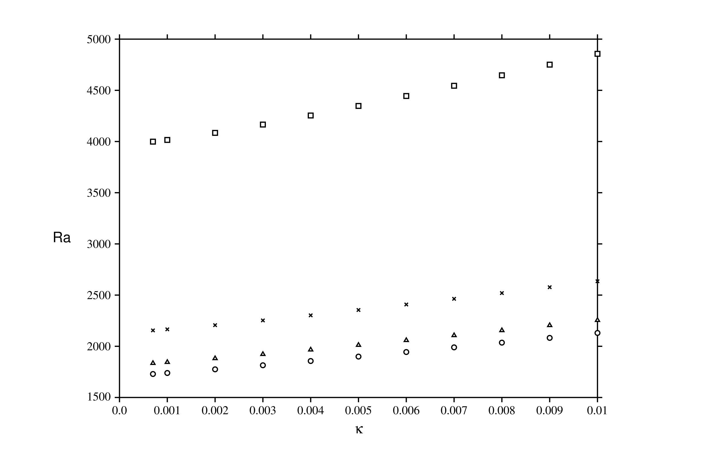
Figure 1: Graph of $Ra$ versus $\kappa$. $\Box$ denotes $\xi=0.01$; $\times$ denotes $\xi=10^{-3}$; $\triangle$ denotes $\xi=10^{-4}$. $\circ$ denotes $\xi=10^{-6}$; $\kappa$ runs from $0.0007$ to 0.01.

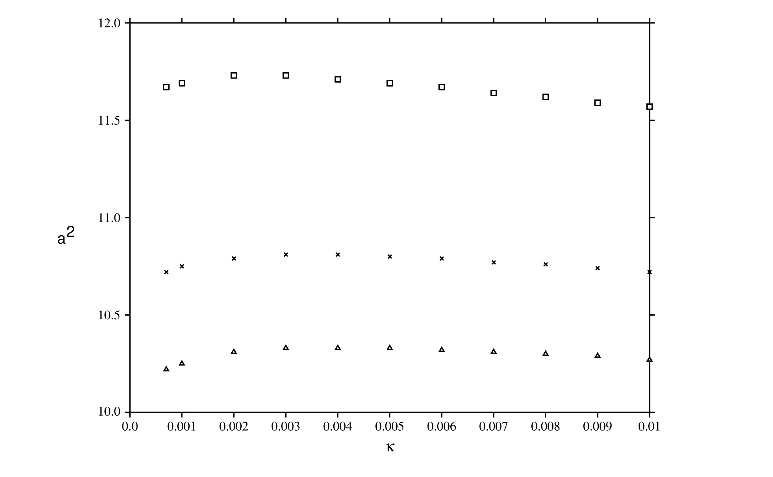
Figure 2: Graph of $a^{2}$ versus $\kappa$. $\Box$ denotes $\xi=0.01$; $\times$ denotes $\xi=10^{-3}$; $\triangle$ denotes $\xi=10^{-4}$. $\kappa$ runs from $0.0007$ to 0.01.

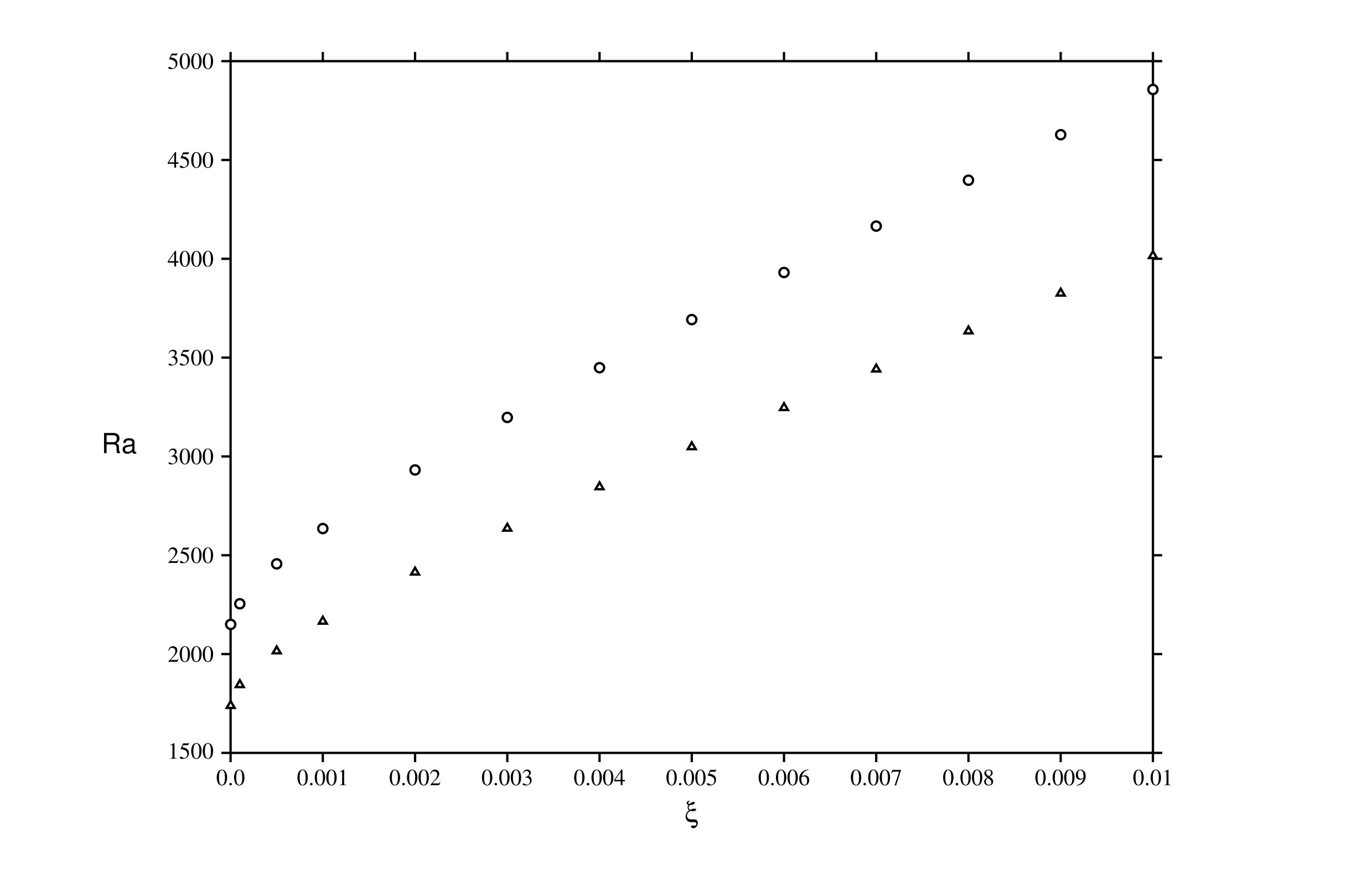
Figure 3: Graph of $Ra$ versus $\xi$. $\circ$ denotes $\kappa=0.01$; $\triangle$ denotes $\kappa=10^{-3}$; $\xi$ runs from $10^{-6}$ to 0.01.

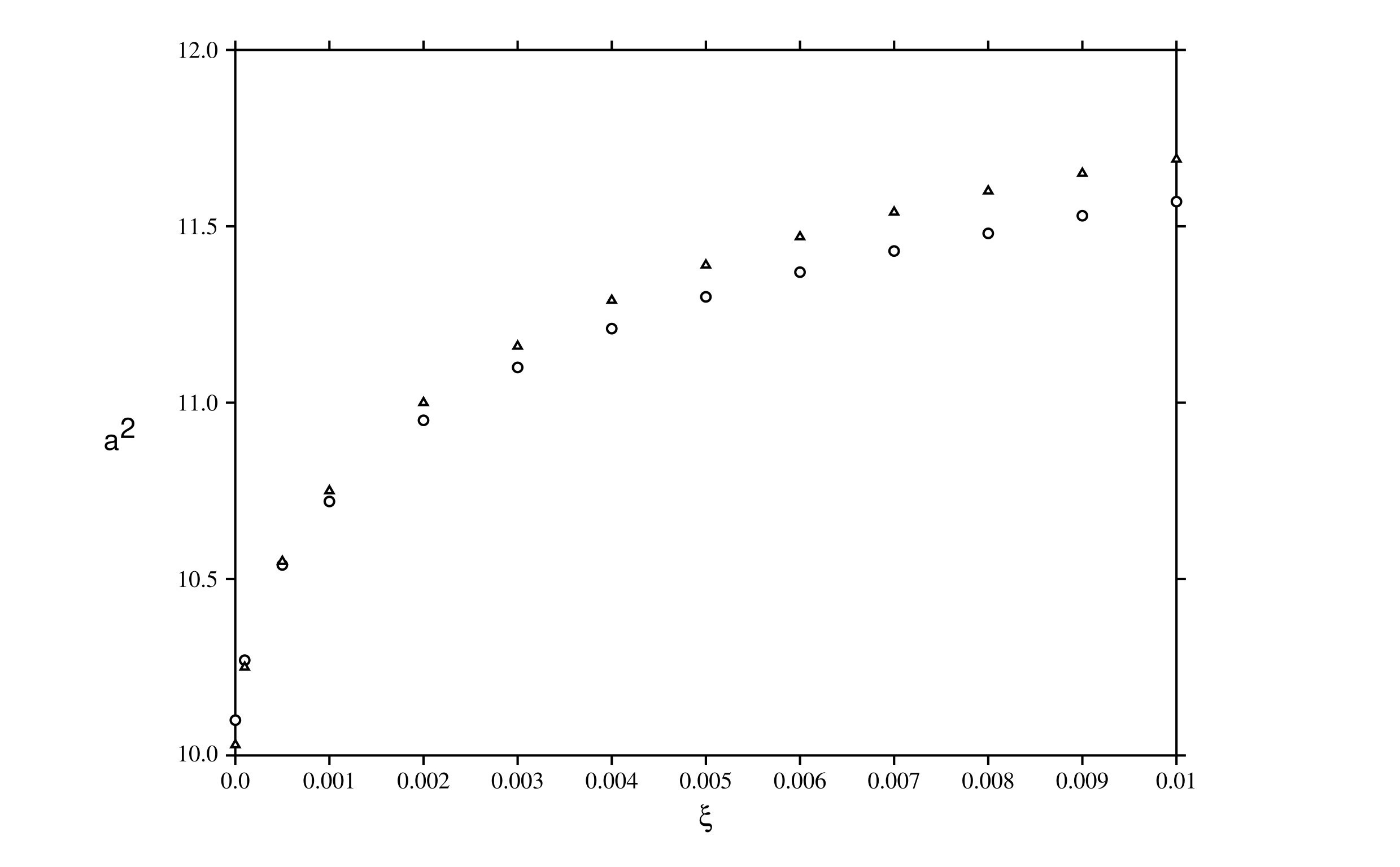
Figure 4: Graph of $a^{2}$ versus $\xi$. $\circ$ denotes $\kappa=0.01$; $\triangle$ denotes $\kappa=10^{-3}$; $\xi$ runs from $10^{-6}$ to 0.1.

8 Conclusions

We have investigated a model for thermal convection employing a generalized Navier-Stokes theory which includes bi-Laplacian terms of both the velocity and temperature fields. Such a hydrodynamic model is physically very relevant in current research since, for example, [25, 26] and [24] argue that such extra spatial derivatives will be important when the molecular structure of the fluid involves long molecules. In addition, such a model fits well in the rapidly expanding industry of microfluidics where length scales are very small, see [19]. We have incorporated higher gradients of temperature into the model and this fits in with similar research in viscoelasticity by [18]. It has been shown that the results of linear instability are practically the same as those found from a global nonlinear energy stability analysis. This is very important and demonstrates that the key physics is incorporated by utilizing linear instability theory.

Currently energy production is a vital topic affecting everyone. In this regard [59] describe a new method which involves heating and cooling a ceramic plate positioned above a container of oil which is undergoing convective thermal motion. The variation of temperature in the ceramic plate produces electricity by means of the the pyroelectric effect. It is interesting to ask whether a fluid with long molecules, or a suspension, in a situation where micro-length scales dominate, would improve this technique of generating electricity. This could be a genuine use for the theory proposed here.

Another relevant area in renewable energy is solar pond technology. Recent research is adding phase change and other materials to salt water to increase efficiency of the solar pond distillation and electricity production, cf. [34], [58]. Addition of such materials will change the molecular structure of the fluid and is likely to be suited to higher order velocity and temperature gradients. The work described herein is suitable for a description of a solar pond since it predicts a significantly increased critical Rayleigh number. This means that the threshold before convective instability begins is larger and this is highly useful in a solar pond where one does not wish convective motion to ensue.

Thermal convection in nanofluids is very topical in heat transfer and renewable energy research, see e.g. [11]. A nanofluid is typically a suspension of tiny particles of a metallic oxide in a carrier fluid and there is definite evidence that a suspension does not behave like a Navier-Stokes fluid, see e.g. [32]. A copper oxide nanofluid suspension contains particles of the shape of a prolate spheroid of aspect ratio 3, see [32]. Such a molecular liquid is known to display behaviour not commensurate with Navier-Stokes theory, see e.g. [52], where a flattened velocity profile is observed in Poiseuille flow instead of the parabolic one of classical fluid mechanics. The higher order velocity and temperature gradient theory described here does not suffer from the drawback of a parabolic profile. Hence, we believe the theory proposed here is suitable for the basis of a proper description of convection in a nanofluid suspension.

To conclude we observe that stimulating recent work of [37], [36] has analysed interesting attractors and behaviour for ordinary differential equation systems derived from double diffusive convection using Navier-Stokes theory. It is an interesting question to analyse how the inclusion of higher spatial gradients of both velocity and temperature would affect the attractor behaviours.

Acknowledgments. The authors would like to thank Marco Degiovanni for providing some helpful suggestions. The work of BS was supported by an Emeritus Fellowship of the Leverhulme Trust, EM-2019-022/9. GG, AG, CL, AM and AM are supported by Gruppo Nazionale per la Fisica Matematica (GNFM) of Istituto Nazionale di Alta Matematica (INdAM).

References

- [1] M. Aouadi, F. Passarella, and V. Tibullo. Exponential stability in Mindlin’s form II gradient thermoelasticity with microtemperatures of type III. Proc. Roy. Soc. London A, 476:20200459, 2020.
- [2] A. Barletta. The Boussinesq approximation for buoyant flows. Mech. Research Comm., 124:103939, 2022.
- [3] N. Bazarra, J. R. Fernández, and R. Quintanilla. Lord - Shulman thermoelasticity with microtemperatures. Appl. Math. Optimization, 84:1667–1685, 2021.
- [4] J. J. Bissell. Thermal convection in a magnetized conducting fluid with the Cattaneo - Christov heat flow model. Proc. Roy. Soc. London A, 472:20160649, 2016.
- [5] J. L. Bleustein and A. E. Green. Dipolar fluids. Int. J. Engng. Sci., 5:323–340, 1967.
- [6] D. Bresch, E. H. Essoufi, and M. Sy. Effect of density dependent viscosities on multiphasic incompressible fluid models. J. Math. Fluid Mech., 9:377–397, 2007.
- [7] D. Bresch, M. Gisclon, I. Lacroix Violet, and A. Vasseur. On the exponential decay for compressible Navier -Stokes - Korteweg equations with a drag term. J. Math. Fluid Mech., 24:11, 2022.
- [8] H. Brezis. Functional analysis, Sobolev spaces and partial differential equations, volume 2. Springer, 2011.
- [9] F. Capone, R. De Luca, and P. Vadasz. Onset of thermosolutal convection in rotating horizontal nanofluid layers. Acta Mech., 233:2237–2247, 2022.
- [10] S. Chandrasekhar. Hydrodynamic and hydromagnetic stability. Dover, New York, 1981.
- [11] M. H. Chang and A. C. Ruo. Rayleigh - Bénard instability in nanofluids: effect of gravity settling. J. Fluid Mech., 950:A37, 2022.
- [12] C. I. Christov. On a higher gradient generalization of Fourier’s law of heat conduction. In American Institute of Physics Conference Proceedings, volume 346, pages 11–22, 2007.
- [13] I. C. Christov, V. Cognet, T. C. Shidhore, and H. A. Stone. Flow rate - pressure drop relation for deformable shallow microfluidic channels. J. Fluid Mech., 814:267–286, 2018.
- [14] P. D. Damázio, P. Manholi, and A. L. Silvestre. Lq theory of the Kelvin - Voigt equations in bounded domains. J. Differential Equations, 260:8242–8260, 2016.
- [15] M. Degiovanni, A. Marzocchi, and S. Mastaglio. Existence, Uniqueness, and Regularity for the Second–Gradient Navier–Stokes Equations in Exterior Domains, pages 181–202. Springer International Publishing, 2020.
- [16] I. A. Eltayeb. Convective instabilities of Maxwell - Cattaneo fluids. Proc. Roy. Soc. London A, 473:20160712, 2017.
- [17] M. Fabrizio, F. Franchi, and R. Nibbi. Second gradient Green - Naghdi type thermoelasticity and viscoelasticity. Mech. Res. Communications, 126:104014, 2022.
- [18] M. Fabrizio, F. Franchi, and R. Nibbi. Nonlocal continuum mechanics structures: The virtual powers method vs. the extra fluxes topic. J. Thermal Stresses, 46:75–87, 2023.
- [19] E. Fried and M. E. Gurtin. Tractions, balances, and boundary conditions for nonsimple materials with application to flow at small length scales. Arch. Rational Mech. Anal., 182:513–554, 2006.
- [20] G.P. Galdi, D.D. Joseph, L. Preziosi, and S. Rionero. Mathematical problems for miscible, incompressible fluids with korteweg stresses. European Journal of Mechanics B-fluids, 10:253–267, 1991.
- [21] G.P. Galdi and S. Rionero. Weighted energy methods in linear elastodynamics in unbounded domains, pages 108–119. Springer Berlin Heidelberg, Berlin, Heidelberg, 1985.
- [22] G. G. Giusteri, A. Marzocchi, and A. Musesti. Nonsimple isotropic incompressible linear fluids surrounding one - dimensional structures. Acta Mech., 217:191–204, 2011.
- [23] T. Goudon and A. Vasseur. On a model for mixture flows: derivation, dissipation and stability properties. Arch. Rational Mech. Anal., 220:1–35, 2016.
- [24] A. E. Green, P. M. Naghdi, and R. S. Rivlin. Directors and multipolar displacements in continuum mechanics. Int. J. Engng. Sci., 2:611–620, 1965.
- [25] A. E. Green and R. S. Rivlin. Multipolar continuum mechanics. Arch. Rational Mech. Anal., 17:113–147, 1964.
- [26] A. E. Green and R. S. Rivlin. The relation between director and multipolar theories in continuum mechanics. ZAMP, 18:208–218, 1967.
- [27] F. Guillén González, P. Damázio, and M. A. Rojas Medar. Approximation by an iterative method for regular solutions for incompressible fluids with mass diffusion. J. Math. Anal. Appl., 326:468–487, 2007.
- [28] D. W. Hughes, M. R. E. Proctor, and I. A. Eltayeb. Maxwell - Cattaneo double diffusive convection: limiting cases. J. Fluid Mech., 927:A13, 2021.
- [29] D. Iesan. Thermal stresses that depend on temperature gradients. ZAMP, 74:138, 2023.
- [30] A. Jabour and A. Bondi. Existence and uniqueness of strong solutions to the density - dependent incompressible Navier - Stokes - Korteweg system. J. Math. Anal. Appl., 460:https://doi.org/10.1016/j.jmaa.2022.12661, 2022.
- [31] V. K. Kalantarov and E. S. Titi. Global stabilization of the Navier - Stokes - Voigt and the damped nonlinear wave equations by a finite number of feedback controllers. Discrete and Continuous Dynamical Systems B, 23:1325–1345, 2018.
- [32] K. Kwak and C. Kim. Viscosity and thermal conductivity of copper oxide nanofluid dispersed in ethylene glycol. Korea Aust. Rheol. J., 17:35–40, 2005.
- [33] O. A. Ladyzhenskaya. On some gaps in two of my papers on the Navier - Stokes equations and the way of closing them. J. Math. Sciences, 115:2789–2791, 2003.
- [34] I. Mahfoudh, P. Principi, R. Fioretti, and M. Safi. Experimental studies on the effect of using phase change materials in a salinity - gradient solar pond under a solar simulator. Solar Energy, 186:335–346, 2019.
- [35] C. B. Moler and G. W. Stewart. An algorithm for the generalized matrix eigenvalue problem . Technical report, Univ. Texas at Austin, 1971.
- [36] S. Moon, J. J. Baik, J. M. Seo, and B. S. Han. Effects of density - affecting scalar on the onset of chaos in a simplified model of thermal convection: a nonlinear dynamical perspective. Eur. Phys. J. Plus, 136:92, 2021.
- [37] S. Moon, J. M. Seo, B. S. Han, J. Park, and J. J. Baik. A physically extended Lorenz system. Chaos, 29:063129, 2019.
- [38] A. Musesti. Isotropic linear constitutive relations for nonsimple fluids. Acta Mech., 204:81–88, 2009.
- [39] G. Nika. A gradient system for a higher gradient generalization of Fourier’s law of heat conduction. Modern Physics Letters B, 37:2350011, 2023.
- [40] G. Nika and A. Muntean. Hypertemperature effects in heterogeneous media and thermal flux at small length scales. Networks and Heterogeneous Media, 12:1207–1225, 2022.
- [41] L. E. Payne and B. Straughan. A naturally efficient numerical technique for porous convection stability with non-trivial boundary conditions. Int. J. Numerical and Analytical Methods in Geomechanics, 24:815–836, 2000.
- [42] S. Rionero. Metodi variazionali per la stabilità asintotica in media in magnetoidrodinamica. Annali di Matematica pura ed applicata, 78:339–364, 1968.
- [43] A. Samanta. Linear stability of a plane Couette - Poiseuille flow overlying a porous layer. Int. J. Multiphase Flow, 123:103160, 2020.
- [44] J. Slomka and J. Dunkel. Generalized Navier - Stokes equations for active suspensions. Eur. Phys. J. Special Topics, 224:1349–1358, 2015.
- [45] V. K. Stokes. Couple stresses in fluids. Phys. Fluids, 9:1709–1715, 1966.
- [46] B. Straughan. Competitive double diffusive convection in a Kelvin - Voigt fluid of order one. Appl. Math. Optimization, 84:631–650, 2021.
- [47] B. Straughan. Thermosolutal convection with a Navier - Stokes - Voigt fluid. Appl. Math. Optimization, 83:2587–2599, 2021.
- [48] B. Straughan. Effect of temperature upon double diffusive convection in Navier - Stokes - Voigt models with Kazkhikov - Smagulov and Korteweg terms. Appl. Math. Optimization, 87:54, 2023.
- [49] B. Straughan. Thermal convection in a higher gradient Navier - Stokes fluid. European Physical Journal Plus, 138:60, 2023.
- [50] Roger Temam. Infinite-dimensional Dynamical Systems in Mechanics and Physics, volume 68. American Mathematical Soc., 1997.
- [51] Roger Temam. Navier-Stokes equations: theory and numerical analysis, volume 343. American Mathematical Soc., 2001.
- [52] K. P. Travis, B. D. Todd, and D. J. Evans. Poiseuille flow of molecular liquids. Physica A, 240:315–327, 1997.
- [53] C. C. Wang and F. Chen. The bimodal instability of thermal convection in a tall vertical annulus. Phys. Fluids, 34:104102, 2022.
- [54] C. C. Wang and F. Chen. On the double - diffusive layer formation in the vertical annulus driven by radial thermal and salinity gradients. Mech. Res. Comm., 100:103991, 2022. https://doi.org/10.1016/j.mechrescom.2022.103991.
- [55] T. Wang. Unique solvability for the density - dependent incompressible Navier - Stokes - Korteweg system. J. Math. Anal. Appl., 455:606–618, 2017.
- [56] X. Wang and I. C. Christov. Theory of flow induced deformation of shallow compliant microchannels with thick walls. Proc. Roy. Soc. London A, 475:20190513, 2019.
- [57] X. Wang, S. D. Pande, and I. C. Christov. Flow rate - pressure drop relations for new configurations of slender compliant tubes arising in microfluidics. Mech. Research Comm., 126:104016, 2022.
- [58] J. Yu, Q. Wu, L. Bu, Z. Nie, Y. Wang, J. Zhang, K. Zhang, N. Renchen, T. He, and Z. He. Experimental study on improving lithium extraction efficiency of salinity - gradient solar pond through sodium carbonate addition and agitation. Solar Energy, 242:364–377, 2022.
- [59] Fatima Zahra El fatnani, Daniel Guyomar, Fouad Belhora, M’hammed Mazroui, Yahia Boughaleb, and Abdelowahed Hajjaji. A new concept to harvest thermal energy using pyroeletric effect and rayleigh-benard convections. The European Physical Journal Plus, 131:1–9, 2016.
- [60] A. V. Zvyagin. Solvability for equations of motion of weak aqueous polymer solutions with objective derivative. Nonlinear Analysis, 90:70–85, 2013.