Gas Source Localization Using Physics-Guided Neural Networks

Abstract

This work discusses a novel method for estimating the location of a gas source based on spatially distributed concentration measurements taken, e.g., by a mobile robot or flying platform that follows a predefined trajectory to collect samples. The proposed approach uses a Physics-Guided Neural Network to approximate the gas dispersion with the source location as an additional network input. After an initial offline training phase, the neural network can be used to efficiently solve the inverse problem of localizing the gas source based on measurements. The proposed approach allows avoiding rather costly numerical simulations of gas physics needed for solving inverse problems. Our experiments show that the method localizes the source well, even when dealing with measurements affected by noise.

I Introduction

The problem of Gas Source Localization (GSL) (e.g., of a gas leak) by means of measurements taken by mobile agents has received increasing attention in the last decades due to rapid improvements in robotics and gas sensor technology. While biologically inspired localization approaches, such as chemotaxis or anemotaxis, have initially served as simple guiding principles, these strategies have been found to be not robust enough for efficient source localization [1, Sec. 4.1]. More recent probabilistic model-based approaches, such as infotaxis, have proved more reliable in patchy and turbulent regimes. However, they rely on assumptions on the source distribution, making them highly dependent on prior knowledge [2, Sec. 6]. Further, the incorporated models often come with high computational costs. For a detailed review of different GSL-approaches, we refer to [1] and the references therein.

In the present work, we propose a strategy which approximates the complex gas dispersion physics through the use of an easy-to-evaluate neural network. More precisely, a Physics-Guided Neural Network (PGNN) [3, Secs. 1,2] is used as a surrogate model for the advection-diffusion Partial Differential Equation (PDE). This network is trained to learn and efficiently emulate the complicated functional dependency between the spatial gas concentration and the source location.

Our surrogate model approach offers several advantages: First, it is flexible and can be applied to various types of PDEs with different boundary conditions and parameters. Second, our surrogate model can be differentiated easily with respect to the source location, thanks to automatic differentiation libraries. This makes the model extremely useful in the inverse problem setting that requires a gradient-based numerical optimization method. Third, the computationally expensive network training can be done once offline. Afterwards, the network can be used for solving GSL-problems with different observations, without the need for retraining or a costly PDE-solver. This opens up the possibility for real-time applications, even those using hardware-constrained robots. Lastly, our method is also robust to noisy measurements and, thus, able to handle inaccuracies caused by sensor limitations.

II Methodology

II-A Gas Model

We assume that the gas occupies the spatial domain $\Omega=($0\text{\,}\mathrm{km}$,$1\text{\,}\mathrm{km}$)\times($0\text{\,}\mathrm{km}$,$1\text{\,}\mathrm{km}$)$. On the set $\Omega$, we model the gas spread by the linear advection-diffusion PDE. For the sake of simplicity, we consider a time-invariant (equilibrium) problem with homogeneous Dirichlet BCs. This is given by the PDE

$$\partial_{t}u(\boldsymbol{x})=\kappa\Delta u(\boldsymbol{x})-\boldsymbol{v}\cdot\nabla u(\boldsymbol{x})+s(\boldsymbol{x}) =0 \text{in }\Omega,$$ (1)

$$u(\boldsymbol{x}) =0 \text{on }\partial\Omega.$$

Here, $\partial\Omega$ is the boundary of $\Omega$, $u\colon\Omega\to\mathbb{R}$ is the gas concentration, $s$ is a source term (either a real-valued function or a measure on $\Omega$), $\kappa=$1\text{\,}{\mathrm{km}}^{2}\text{\,}{\mathrm{h}}^{-1}$$ is the diffusion coefficient, and $\boldsymbol{v}=[$3\text{\,}\mathrm{km}\text{\,}{\mathrm{h}}^{-1}$,$3\text{\,}\mathrm{km}\text{\,}{\mathrm{h}}^{-1}$]^{\top}$ is the advection velocity. We assume a uniform (known) wind flow.

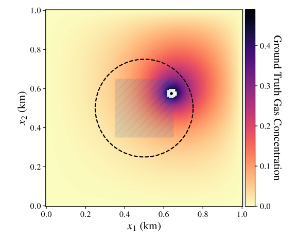
Figure 1: Problem setup. The gas concentration field is shown as an example. (A ball of radius $20\text{\,}\mathrm{m}$ around $\boldsymbol{p}$ is excluded to avoid the singularity.) The dotted black circle represents $D_{\mathrm{O}}$, the trajectory of the observations. The source location $\boldsymbol{p}$ is marked by a black dot and the set $\mathcal{P}$ of possible source positions by the blue hatched region.

Since we are interested in GSL, we assume that there is a location parameter set $\mathcal{P}=[$0.35\text{\,}\mathrm{km}$,$0.65\text{\,}\mathrm{km}$]\times[$0.35\text{\,}\mathrm{km}$,$0.65\text{\,}\mathrm{km}$]\subset\Omega$ which fully represents all possible points $\boldsymbol{p}\in\mathbb{R}^{2}$ where the source could be located. We shall use $s_{\boldsymbol{p}}$ and $u_{\boldsymbol{p}}$ to denote the source term and the gas concentration field associated with the source position $\boldsymbol{p}$, respectively. That is, $u_{\boldsymbol{p}}$ is the solution of (1) with source term $s_{\boldsymbol{p}}$.

For the purposes of this paper, we restrict our attention to ideal point sources, i.e., Dirac delta distributions. Keeping with previous notation, this means that we consider source terms of the form $s_{\boldsymbol{p}}:=\delta_{\boldsymbol{p}}$, $\boldsymbol{p}\in\mathcal{P}$. Note that, for such $s_{\boldsymbol{p}}$, the solutions $u_{\boldsymbol{p}}$ of (1) possess a singularity at $\boldsymbol{p}$. This means in particular that $u_{\boldsymbol{p}}$ cannot be evaluated at $\boldsymbol{p}$.

II-B Source Localization Problem

In a source localization problem governed by (1), the goal is to identify the location $\boldsymbol{p}\in\mathcal{P}$ associated with the source term $s_{\boldsymbol{p}}$ from measurements of $u_{\boldsymbol{p}}$ taken by a mobile robot on an observation domain $D_{\mathrm{O}}\subset\Omega$. The set $D_{\mathrm{O}}$ can be considered as the robot trajectory in the region of interest; cf. Fig. 1.

We suppose that the gas concentration measurements are taken at $N_{\mathrm{O}}$ observation points $\boldsymbol{x}_{1},...,\boldsymbol{x}_{N_{\mathrm{O}}}\in D_{\mathrm{O}}$. A measurement $y_{j}$ at $\boldsymbol{x}_{j}$ is the gas concentration $u_{\boldsymbol{p}}(\boldsymbol{x}_{j})$ perturbed by zero-mean additive Gaussian noise with standard deviation $\sigma$. To avoid evaluating the solution of (1) at its singularity, we henceforth assume that $\mathcal{P}\cap D_{\mathrm{O}}=\emptyset$. We remark that this restriction can be avoided by replacing the point sources $\delta_{\boldsymbol{p}}$ with a suitable mollification.

To determine the source location based on measurements $y_{1},...,y_{N_{\mathrm{O}}}$, we consider the minimization problem

$$\min_{\boldsymbol{p}^{\prime}\in\mathcal{P}}\leavevmode\nobreak\ \mathcal{J}(\boldsymbol{p}^{\prime}):=\sum_{j=1}^{N_{\mathrm{O}}}(y_{j}-u_{\boldsymbol{p}^{\prime}}(\boldsymbol{x}_{j}))^{2}.$$ (2)

Note that standard optimization algorithms for (2) require evaluations of the objective $\mathcal{J}$ and its derivatives at numerous points $\boldsymbol{p}^{\prime}$. Due to the definition of $u_{\boldsymbol{p}^{\prime}}$, for each of these evaluations, one has to solve the PDE (1) with parameter $\boldsymbol{p}^{\prime}$ and, in the case that derivatives are required, an additional adjoint PDE. This is often computationally prohibitive, in particular if the aim is to solve (2) with limited hardware, e.g., directly on-board a robot. The main idea of our approach is to resolve this problem by setting up a reusable neural network model for the functional dependency $(\boldsymbol{x},\boldsymbol{p})\mapsto u_{\boldsymbol{p}}(\boldsymbol{x})$ which is trained once offline, i.e., we use a surrogate for $u_{\boldsymbol{p}^{\prime}}$ in (2).

II-C Neural Network (NN) Surrogate

II-C1 Network Architecture

As our surrogate model for the functional dependency $(\boldsymbol{x},\boldsymbol{p})\mapsto u_{\boldsymbol{p}}(\boldsymbol{x})$, we consider a Multilayer Perceptron (MLP), a fully-connected feed-forward neural network. A popular architecture for an $L$-layer MLP $\mathcal{N}\colon\mathbb{R}^{n_{\text{in}}}\to\mathbb{R}^{n_{\text{out}}}$ with input variable $\boldsymbol{z}$ is the following:

$$\boldsymbol{l}_{0}:=\boldsymbol{z},\quad\boldsymbol{l}_{k} :=\rho(\boldsymbol{W}_{k}\boldsymbol{l}_{k-1}+\boldsymbol{b}_{k}),\,\,k=1,...,L-1,$$ (3)

$$\mathcal{N}(\boldsymbol{z}) :=\boldsymbol{W}_{L}\boldsymbol{l}_{L-1}+\boldsymbol{b}_{L}.$$

Here, $\boldsymbol{W}_{k}\in\mathbb{R}^{n_{k}\times n_{k-1}},\boldsymbol{b}_{k}\in\mathbb{R}^{n_{k}}$ are the $k$-th layer’s weight matrix and bias vector, respectively, with $n_{0},...,n_{L}\in\mathbb{N}$ the number of neurons at each layer ($n_{0}=n_{\text{in}}$, $n_{L}=n_{\text{out}}$), and $\rho\colon\mathbb{R}\to\mathbb{R}$ is the nonlinear activation function, evaluated componentwise when applied to a vector. We note that the definition (3) follows common practice and has the last network layer as a scaling layer without an activation function.

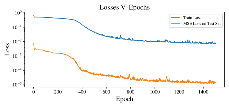
Figure 2: The surrogate model’s performance over its training period. Blue: $H_{1}$-loss on training set. Orange: Mean Square Error (MSE) of function values on test set (withheld from NN-training).

In our application, the network concatenates both the spatial coordinate $\boldsymbol{x}\in\Omega$ and the source location $\boldsymbol{p}\in\mathcal{P}$ as a single input $\boldsymbol{z}:=[\boldsymbol{x};\boldsymbol{p}]$, and it outputs an approximation of $u_{\boldsymbol{p}}(\boldsymbol{x})$. This means $n_{\text{in}}=n_{0}=2+2=4,n_{\text{out}}=n_{L}=1$.

For the numerical experiments in this paper, we used a network with 5 layers, 30 neurons in each hidden layer ($n_{1},...,n_{4}=30$), and the softplus activation function.

II-C2 Enforcing Boundary Conditions

We use the hard-enforcement approach suggested in [4] to realize the BCs. Our approximator multiplies the MLP output $\mathcal{N}$ from (3) by a cutoff function $\psi$ which vanishes on the spatial boundary $\partial\Omega$. This ensures homogeneous Dirichlet BCs. Thus, we define

$$\tilde{u}_{\boldsymbol{p}}(\boldsymbol{x}):=\psi(\boldsymbol{x})\mathcal{N}([\boldsymbol{x};\boldsymbol{p}]).$$ (4)

As the function $\psi$, we use the so-called “$R$-$m$ approximate distance function” to the boundary $\partial\Omega$ [4].

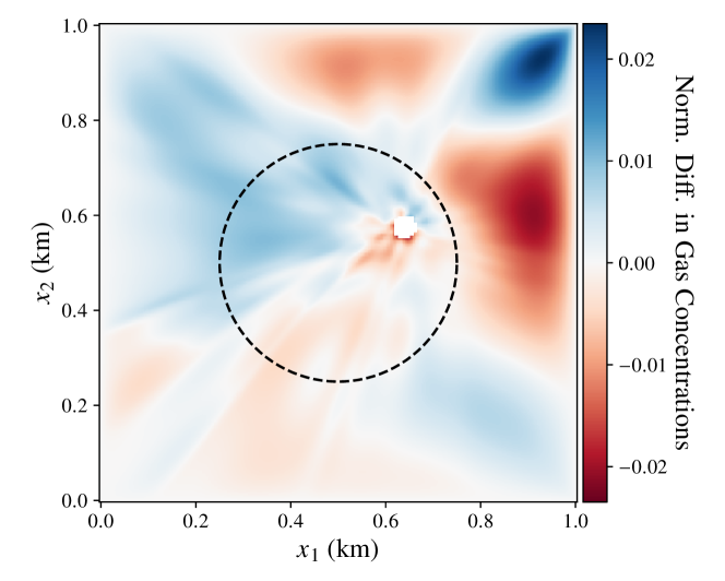
(a)

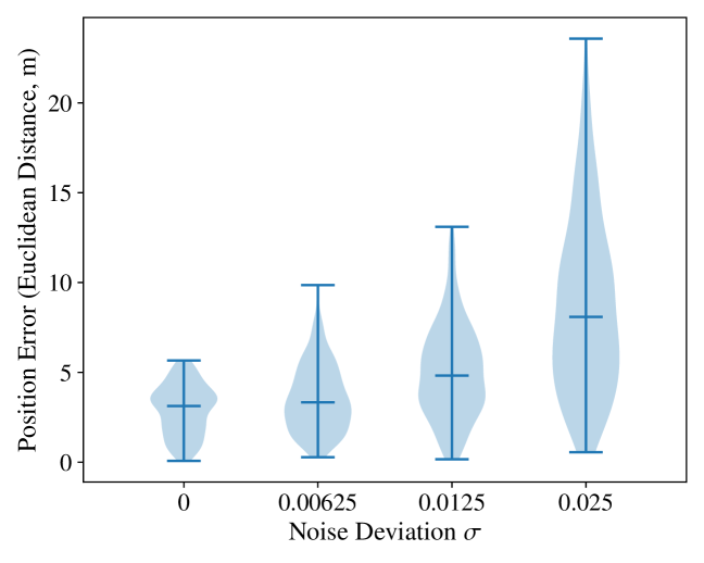
(b)

Figure 3: NN training results. Fig. (a) shows the difference between the NN-surrogate $\tilde{u}_{\boldsymbol{p}}$ and the reference solution $u_{\boldsymbol{p}}$ in $\Omega$, normalized by the maximum value of $u_{\boldsymbol{p}}$ excluding a ball of radius $20\text{\,}\mathrm{m}$ around the source, in the situation of Fig. 1. Fig. (b) shows the (Euclidean) position error of the location $\boldsymbol{p}$ calculated by solving (2) with our NN-surrogate approach with increasing amounts of White Gaussian Noise.

II-C3 Network Training

To train the NN-surrogate $\tilde{u}_{\boldsymbol{p}}$, we use a physics-guided approach. This supervised learning method compares the network output and its spatial gradients with a reference solution and attempts to make them as similar as possible. We thus define the Physics-Guided $H_{1}$-Loss by

$$L_{\textbf{PG}}:=\frac{1}{N_{t}}\sum_{i=1}^{N_{t}}\left[(\tilde{u}_{\boldsymbol{p}_{i}}-u_{\boldsymbol{p}_{i}})(\boldsymbol{q_{i}})\right]^{2}+\lVert(\nabla\tilde{u}_{\boldsymbol{p}_{i}}-\nabla u_{\boldsymbol{p}_{i}})(\boldsymbol{q_{i}})\rVert_{2}^{2}.\vspace{-0.1cm}$$

Here, $\tilde{u}_{\boldsymbol{p}}$ is the model in (4), $u_{\boldsymbol{p}}$ denotes a reference solution computed, e.g., by the Finite Element Method (FEM), $\nabla$ is the spatial gradient, $\{(\boldsymbol{p}_{i},\boldsymbol{q}_{i})\}\subset\mathcal{P}\times\Omega$ is a set of $N_{t}$ evaluation points, and $L_{\textbf{PG}}$ is understood as a function of the weights and biases in $\mathcal{N}$. Note that the $H_{1}$-loss, as opposed to the naive Mean Square Error (MSE), includes information about the gradient of the reference solution.

In our numerical experiments, we used $N_{t}$ = 80000 points $(\boldsymbol{p}_{i},\boldsymbol{q}_{i})$ in $L_{\textbf{PG}}$, sampled randomly from $\mathcal{P}\times\Omega$. Since $u_{\boldsymbol{p}}$ has a singularity at $\boldsymbol{p}$, we excluded points $\boldsymbol{q}_{i}$ with a distance smaller than $0.02\text{\,}\mathrm{km}$ from the source location $\boldsymbol{p}_{i}$. For the generation of the reference data, we used a discretization based on the FEniCS library [5] on a Friedrichs–Keller triangulation on a $241\times 241$ grid and linear Lagrangian elements. The NN-surrogate was trained and implemented in Python using the Pytorch library [6]. We used the ADAM Optimizer with learning rate $l=10^{-3}$ to train $\tilde{u}_{\boldsymbol{p}}$ over 1500 epochs of the dataset. We additionally computed the MSE on another set of 20000 test points randomly sampled from $\mathcal{P}\times\Omega$, excluding singularities, to check the surrogate’s generalization performance. The training results can be seen in Fig. 2.

II-D Optimization Algorithm

Once the NN-surrogate $\tilde{u}_{\boldsymbol{p}}$ has been trained, the inverse problem (2), with $u_{\boldsymbol{p}}$ replaced by $\tilde{u}_{\boldsymbol{p}}$, can be solved with standard optimization algorithms. In our experiments, we used the LBFGS-B method [7] for this purpose. The method had information about the gradients $\nabla_{\boldsymbol{p}}\tilde{u}_{\boldsymbol{p}}$ via the automatic differentiation functionalities of the Pytorch library [6]. Note that the optimization step only requires gradients of the surrogate model $\tilde{u}_{\boldsymbol{p}}$. Measurements of the concentration gradients do not have to be taken in our GSL-approach and we do not require that the actual concentration field is smooth. (It should, of course, be such that it is sufficiently well described by (1).)

III Results

To test our method’s performance, we first checked that the surrogate model provides a sensible approximation. In addition to the loss metric in the training curve, we used a comparison with a reference solution for this purpose. In Fig. 3(a), we see the difference between modeled values and ground truth for a fixed source position, normalized by the maximum concentration value of the reference function outside of its singular region. We can see that the difference is within 2% of the maximum source value in all of $\Omega$.

Next, we tested the performance of our PGNN in the GSL-problem (2). To do this, we chose a set $\{\boldsymbol{x}_{j}\}$ of $N_{\mathrm{O}}=100$ evenly spaced points on the circle of radius $0.25\text{\,}\mathrm{km}$ around $($0.5\text{\,}\mathrm{km}$,$0.5\text{\,}\mathrm{km}$)$ as the observation domain $D_{\mathrm{O}}$. Note that this choice of $D_{\mathrm{O}}$ is purely for demonstration purposes. More complicated $D_{\mathrm{O}}$ could be considered here without problems. We then sampled 324 source positions $\boldsymbol{p}$ inside the set $\mathcal{P}$ on a grid. For each of these source positions, first, we used the FEM to compute the ground truth values $y_{j}$ at the observation points $\boldsymbol{x}_{j}$ without noise, and then solved the inverse problem (2), localizing the gas source to get the estimate $\hat{\boldsymbol{p}}$. The source positioning error is measured as $\lVert\boldsymbol{p}-\hat{\boldsymbol{p}}\rVert_{2}$. We additionally repeated these tests, adding white Gaussian noise of standard deviation $\sigma\in\{0.00625,0.0125,0.025\}$ to the observations. Each inverse problem was solved in the span of 1 second.

The results of this survey are depicted in Fig. 3(b) in a violin plot of the error. We can see that, without noise, the network can identify the correct source location up to an error of $6\text{\,}\mathrm{m}$ in the worst case and up to an error of $4\text{\,}\mathrm{m}$ on average. Given that the resolution of the FEM-approximation is $4.14\text{\,}\mathrm{m}$, this performance is close to optimal. Even with additive noise corresponding to $\sim 6\%$ of the highest values encountered on the circle, the solver is still able to give source locations within $28\text{\,}\mathrm{m}$ of the real value. We also notice that the median error (middle line) increases much slower than the maximum error.

IV Conclusion

In this paper, we have demonstrated how PGNNs can be used to solve GSL-problems in an accurate, computationally cheap, and robust manner. Our approach is flexible and offers various possibilities for extensions, e.g., to three dimensions and unknown wind/diffusion parameters. In future work, we plan to include dynamic path optimization techniques and realistic sensor models into our framework. Further open points are the validation of our method in real world experiments and the detailed comparison with existing GSL-techniques—two issues that are beyond the scope of the present paper.

References

- [1] Adam Francis, Shuai Li, Christian Griffiths and Johann Sienz “Gas source localization and mapping with mobile robots: A review” In J. of Field Rob. 39.8, 2022, pp. 1341–1373 DOI: https://doi.org/10.1002/rob.22109
- [2] Tao Jing, Qing-Hao Meng and Hiroshi Ishida “Recent Progress and Trend of Robot Odor Source Localization” In IEEJ Transactions on Electrical and Electronic Engineering 16.7, 2021, pp. 938–953 DOI: https://doi.org/10.1002/tee.23364
- [3] Salah A. Faroughi et al. “Physics-Guided, Physics-Informed, and Physics-Encoded Neural Networks and Operators in Scientific Computing: Fluid and Solid Mechanics” In J. Comput. Inf. Sci. Eng., 2024, pp. 1–45 DOI: 10.1115/1.4064449
- [4] N. Sukumar and Ankit Srivastava “Exact imposition of boundary conditions with distance functions in physics-informed deep neural networks” In Comput. Methods Appl. Mech. Eng. 389, 2022, pp. 114333 DOI: https://doi.org/10.1016/j.cma.2021.114333
- [5] Martin S. Alnaes et al. “The FEniCS Project Version 1.5” In Arch. Num. Softw. 3, 2015 DOI: 10.11588/ans.2015.100.20553
- [6] Adam Paszke et al. “Pytorch: An imperative style, high-performance deep learning library” In Adv. Neural Inf. Process. Syst. 32, 2019
- [7] Richard H. Byrd, Peihuang Lu, Jorge Nocedal and Ciyou Zhu “A limited memory algorithm for bound constrained optimization” In SIAM J. Sci. Comp. 16.5 Society for IndustrialApplied Mathematics Publications, 1995, pp. 1190–1208 DOI: 10.1137/0916069