Geometry and Dynamics of LayerNorm
Abstract
A technical note aiming to offer deeper intuition for the LayerNorm function common in deep neural networks. LayerNorm is defined relative to a distinguished ‘neural’ basis, but it does more than just normalize the corresponding vector elements. Rather, it implements a composition—of linear projection, nonlinear scaling, and then affine transformation—on input activation vectors. We develop both a new mathematical expression and geometric intuition, to make the net effect more transparent. We emphasize that, when LayerNorm acts on an -dimensional vector space, all outcomes of LayerNorm lie within the intersection of an -dimensional hyperplane and the interior of an -dimensional hyperellipsoid. This intersection is the interior of an -dimensional hyperellipsoid, and typical inputs are mapped near its surface. We find the direction and length of the principal axes of this -dimensional hyperellipsoid via the eigen-decomposition of a simply constructed matrix.
I Introduction
LayerNorm is a relatively simple function and so is often taken for granted. But, as one of the few building blocks of modern transformers (and other deep neural networks), it is worth understanding deeply. At the risk of stating things that are obvious, this note aims to very explicitly think through the LayerNorm function, how it maps activations, and the resultant geometry of activations.
LayerNorm acts on each -dimensional activation vector via a nonlinear transformation induced by learned parameters , and fixed small parameter [1, 2]. Let denote the -dimensional vector of all ones in the neural basis. Then LayerNorm can be written as
| (1) |
where denotes the element-wise product (i.e., Hadamard product), the mean neural activation is
| (2) |
and the variance of activations across neurons is
| (3) |
Typically, the gain and bias are learned during training. At the beginning of training, and , and by default. This can alternatively be written in standard matrix-multiplication notation as
| (4) |
where diag is the matrix of all zeros except for the elements of along its diagonal. At the beginning of training, diag is the identity matrix, .
II Decomposing and Visualizing LayerNorm
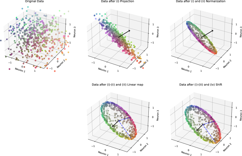
LayerNorm’s net action on the -dimensional activation vector can be thought of as a composition of several other simple functions (i)-(iv), as depicted in Fig. 1. First, LayerNorm performs a linear projection:
-
(i)
Find the mean value of components in the neural basis, and subtract this mean from each component. Notably can be seen as the projection of onto the -dimensional hyperplane perpendicular to .
Here, is the unit vector in the direction of . Note that since . As a consequence, this initial sub-step of LayerNorm projects the activation vector onto a hyperplane that enforces , where is the component of the resultant vector in the neural basis.
Let’s denote the rank- projector . Then we can write the result of sub-step (i) simply as . Note that, as a projector, . Hence, the variance can either be expressed as , or in relation to the square magnitude of since .
Subsequently, LayerNorm performs a nonlinear scaling:
-
(ii)
Scale the magnitude of the resultant vector by , after which it is no larger than . This scales the vector to bring it within the -ball. If is small, then resultant points will be concentrated towards a magnitude of .
After the first two sub-steps (i) and (ii), the activations have been projected and nonlinearly scaled according to:
| (5) |
is a unit vector in the direction of , while the denominator is never smaller than 1. Accordingly, after these first two sub-steps, every input activation vector is mapped into the intersection of (a) the -dimensional hyperplane perpendicular to and (b) the -ball of radius .
After these first two sub-steps, the -sphere and the points it now contains are subsequently (iii) stretched by along the neural-basis directions into a hyperellipsoid, and then (iv) shifted by . Together, sub-steps (iii) and (iv) constitute an affine transformation. The linear transformation (iii)—matrix multiplication by diag—is diagonal in the neural basis, and maps the open -ball containing all points to the interior of an -dimensional hyperellipsoid with principal axes given by the neural basis. Likewise, it stretches and so tilts the intersecting hyperplane that contains all relevant points. The bias (iv) simply shifts the entire hyperellipsoid by .
We can now combine all these sub-steps to re-express LayerNorm as
| (6) |
where we have defined the projector . This expression has the advantage of making all -dependence explicit, while highlighting the projection, scaling, and subsequent affine transformation.
The sequence of sub-steps building up the dynamics and geometry of LayerNorm is depicted in Fig. 1. Although LayerNorm is usually used in high-dimensional vector spaces, it is instructive to visualize and understand how it would operate in three dimensions, as shown, from which higher-dimensional behavior can be both intuitively and rigorously extrapolated.
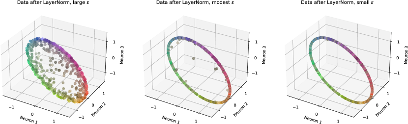
In particular, when LayerNorm acts on an -dimensional vector space, all outcomes of LayerNorm lie within the intersection of an -dimensional hyperplane and an -dimensional hyperellipsoid. This intersection is itself a hyperellipsoid, now of dimension . After a sprinkling of points is transformed by LayerNorm, most of the points subsequently contained in this -dimensional hyperellipsoid are concentrated towards its surface, as shown in Fig. 2.
II.1 Orthogonal subspace
If we subtract the bias, then the image of all activations after LayerNorm is orthogonal to at least one dimension of the vector space. This orthogonal space can be found as the left nullspace of . Let denote the orthonormal neural basis. If the elements of are all non-zero in the neural basis—i.e., if for any —then we find that the orthogonal subspace is the one-dimensional subspace of all vectors proportional to the inverse elements of . I.e., . However, if for at least one , then the number of orthogonal directions is equal to the number of these elements equal to zero, with the orthogonal subspace now given instead by .
II.2 Principal axes
The neural basis forms the principal axes of the -dimensional hyperellipsoid after the -sphere is stretched by . But what are the principal axes of the cross-sectional -hyperellipsoid induced by ? This is a rather more difficult question.
We find that the principal axes are the eigenstates of , with semi-axes of length where is the eigenvalue associated with the eigenstate, , and . As above, contains the reciprocal elements of the scaling vector in the neural basis: .
If has neural-basis components equal to zero, i.e., if for some , then should be interpreted as the square of ’s Drazin inverse [3], while we can then set either or , with . If for any , then has a single zero eigenvalue, with corresponding eigenstate in the subspace orthogonal to LayerNorm’s image.
Lengths of the semi-axes can alternatively be found as where each is an eigenvalue of . However, unlike the use of above, this does not deliver the directions of the principal axes.
III LayerNorm in transformers
In the standard modern transformer architecture, LayerNorm is invoked in two or three different ways, depending on how you count. It is used outside of the residual stream, both before multi-head attention and before the position-wise feed-forward network [4]. And it is used in the final residual stream, just before unembedding.
IV Conclusion
We have investigated LayerNorm as a composition of simpler functions—projection, scaling, and then affine transformation—and have derived an alternative expression (Eq. (6)) for LayerNorm that makes these features more evident. Some work had already been done in this direction—e.g., the projection sub-step implied by LayerNorm was already noted in Refs. [5, 6]. Our short note provides complementary perspective. We included the sometimes non-negligible effect of the small parameter used in the standard PyTorch implementation of LayerNorm. We have also identified the orthogonal subspace to the bias-corrected image of all activations after LayerNorm, which may be useful in understanding how LayerNorm interacts with downstream components of a neural net. Finally, we have identified the principal axes (and their lengths) of the -dimensional hyperellipsoid image of LayerNorm via the eigendecomposition of a simply constructed matrix () that we introduced here.
Better understanding the components of neural networks should help us anticipate their implications, both locally and in composition with other aspects of the network. LayerNorm is a ubiquitous function used in modern neural nets, with more complexity than it initially leads on. We hope this exposition makes it more intuitive, and brings at least another pinhole of light into the black box.
References
- [1] Jimmy Lei Ba, Jamie Ryan Kiros, and Geoffrey E Hinton. Layer normalization. arXiv preprint arXiv:1607.06450, 2016.
- [2] LayerNorm — PyTorch 2.3 documentation. https://pytorch.org/docs/stable/generated/torch.nn.LayerNorm.html. [Accessed 27-04-2024].
- [3] P. M. Riechers and J. P. Crutchfield. Beyond the spectral theorem: Decomposing arbitrary functions of nondiagonalizable operators. AIP Advances, 8:065305, 2018.
- [4] Ruibin Xiong, Yunchang Yang, Di He, Kai Zheng, Shuxin Zheng, Chen Xing, Huishuai Zhang, Yanyan Lan, Liwei Wang, and Tieyan Liu. On layer normalization in the transformer architecture. In International Conference on Machine Learning, pages 10524–10533. PMLR, 2020.
- [5] Shaked Brody, Uri Alon, and Eran Yahav. On the expressivity role of LayerNorm in transformers’ attention. arXiv preprint arXiv:2305.02582, 2023.
- [6] Raul Molina. Traveling words: A geometric interpretation of transformers. arXiv preprint arXiv:2309.07315, 2023.