A MeerKAT Polarization Survey of Southern Calibration Sources

Abstract

We report on full-Stokes L-band observations of 98 MeerKAT calibration sources. Linear polarization is detected in 71 objects above a fractional level of 0.2%. We identify ten sources with strong fractional linear polarization and low Faraday Rotation Measure that could be suitable for wide-band absolute polarization calibration. We detect significant circular polarization from 24% of the sample down to a detection level of 0.07%. Circularly polarized emission is seen only for flat spectrum sources $\alpha>-0.5$.

We compare our polarized intensities and Faraday Synthesis results to data from the NVSS at 1400 MHz and the ATCA SPASS survey at 2300 MHz. NVSS data exists for 54 of our sources and SPASS data for 20 sources. The percent polarization and Rotation Measures from both surveys agree well with our results.

The residual instrumental linear polarization for these observations is measured at 0.16% and the residual instrumental circular polarization is measured at 0.05%. These levels may reflect either instabilities in the relative bandpass between the two polarization channels with either time or antenna orientation, or atmospheric/ionospheric variations with pointing direction. Tracking of the hourly gain solutions on J0408-6545 after transfer of the primary gain solutions suggests a deterioration of the gain stability by a factor of several starting about two hours after sunrise. This suggests that observing during the nighttime could dramatically improve the precision of polarization calibration.

1 Introduction

Radio polarimetry is a powerful probe of cosmic magnetic fields, and is central to science programs on next generation radio facilities and to planning for the Square Kilometre Array (Heald et al., 2020). For telescopes with linear polarized feeds, polarized signals from radio sources are mixed into all correlation products. It is therefore important for both observational planning and precise calibration to have knowledge of the polarization of calibration sources. To this end, we have begun a program to observed the polarization properties of MeerKAT gain calibration sources. In this paper we report on polarization observations of an initial set of 98 MeerKAT gain calibration sources at L-band.

These calibrators were chosen from a list of 448 sources with declinations below +34 degrees. This initial list was made up of sources from the master list of (Dixon, 1970), PKSCAT90 (Wright & Otrupcek, 1990), NVSS (Condon et al., 1998a), SUMSS v 2.1 (Mauch et al., 2008) with additional data from the The Parkes-MIT-NRAO (PNM) surveys (Griffith & Wright, 1993; Condon et al., 1993; Wright et al., 1994; Griffith et al., 1994; Tasker et al., 1994) and SPECFIND (Vollmer et al., 2005a, b, 2010). All these are available on the VizieR database. The list also includes the well known VLA calibrators 3C48 (J0137+3309), 3C138 (J0521+1638), 3C286 (J1331+3030) as well as PKS B1934-638 (J1939-6342), which is the main calibrator for the Australia Telescope National Facility (ATNF). Another incorporated list was made from VLA calibrators with flux densities greater than 2 Jy at L-band and declinations below -20 degrees. Some of the Molonglo Observatory calibrators were also added to the candidate list but these sources did not pass the final criteria. The criteria for the final list being that sources must: 1) have L-band flux densities above 1 Jy, and be stronger than 10 times the background confusion; 2) be no more than $10\%$ resolved; 3) have closure phases less than 5 degrees ($\sim 0.1$ radians); 4) have stable flux densities on year timescales.

2 Observations

The calibration sources were observed with MeerKAT (Jonas & MeerKAT Team, 2016) during one of two observing runs carried out by the SARAO MeerKAT commissioning team. MeerKAT receivers have two orthogonal linear feeds and the correlator produces all four polarization products viz. HH, HV, VH and VV during all observing runs. The first observing run occurred on 19 August 2019 and the second run on 29 August 2020. The first run observed 52 sources in the RA range 11–23 hours, and second run observed 46 sources in the RA range 00-11 hours. Both observing runs were about 12 hours long. Each target source was observed for a short scan of about 5 minutes. The strong unpolarized source J1939-6342 was observed several times during the each run, and the absolute polarization calibrator J1331+3030 (3C286) was observed twice for 5 minutes at the beginning of the first run, and once for 10 minutes at the end of the second run.

3 Calibration and Imaging

The data were processed on the Ilifu cloud using a customized version of the IDIA calibration and imaging pipeline (Collier et al., 2021). The calibration stage of the pipeline utilises CASA processing (The CASA Team et al., 2022). The pipeline partitions the L-band RF into 15 equally-sized sub-spectral windows between 880 MHz to 1680 MHz. Data in frequency ranges with strong persistent RFI (933–960ṀHz, 1163–1299 MHz, and 1525–1630 MHz) are removed at this partition stage. Each spectral window is split into its own multi-MS that is processed concurrently using the SLURM job manager. Following calibration the calibrated data from each spectral window is merged into a single measurement set with calibrated visibilities.

For linear feeds, the linear approximation to the response of the parallel and cross-hand visibilities is given in equations 1-4 below. In these equations we have retained only those leakage terms that multiply Stokes $I$. A more complete set including leakage terms that multiply the source polarization can be found in Hales (2017).

$$V_{xx}=g^{i}_{x}g^{k}_{x}\bigl{(}I+Q\cos 2\psi+U\sin 2\psi\bigr{)}$$ (1)

$$V_{xy}=g^{i}_{x}g^{k}_{y}\bigl{[}(d^{i}_{x}-d^{k}_{y}\ {}^{*})I-Q\sin 2\psi+U\cos 2\psi+jV\bigr{]}$$ (2)

$$V_{yx}=g^{i}_{y}g^{k}_{x}\bigl{[}(d^{k}_{x}\ {}^{*}-d^{i}_{y})I-Q\sin 2\psi+U\cos 2\psi-jV\bigr{]}$$ (3)

$$V_{yy}=g^{i}_{y}g^{k}_{y}\bigl{(}I-Q\cos 2\psi-U\sin 2\psi\bigr{)}$$ (4)

Any polarized signal from the source is present in all four correlations and varies with parallactic angle $\psi$. Precise measurement of the gains and the leakage terms can be achieved using a strong unpolarized source for which the equations reduce to

$$V_{xx}=g^{i}_{x}g^{k}_{x}I$$ (5)

$$V_{xy}=g^{i}_{x}g^{k}_{y}(d^{i}_{x}-d^{k}_{y}\ {}^{*})I$$ (6)

$$V_{yx}=g^{i}_{y}g^{k}_{x}(d^{k}_{x}\ {}^{*}-d^{i}_{y})I$$ (7)

$$V_{yy}=g^{i}_{y}g^{k}_{y}I$$ (8)

These equations cleanly separate the gain solution into the parallel-hand correlations and the leakage into the cross-hand correlations. As a first step in the calibration we use the observations of J1939-6342 to measure the frequency-dependent $g_{x}$ and $g_{y}$ gains. We then apply the gain solutions and derive the leakage terms also using J1939-6342.

All of the target sources are strong compact objects at the phase and pointing centre of the observation. Following the application of gain and leakage solutions from J1939-6342 to each source, gain solutions for each source are derived by running CASA’s gaincal task on each source (essentially a self-calibration assuming a point source model). We use gaincal parameter gaintype = ‘T’, which averages the $xx$ and $yy$ data before solving for the gain. The local residual gain solution for each source therefore does not modify the relative values of $g_{x}$ and $g_{y}$ gains derived from the bandpass calibrator, thus preserving the polarization calibration, and the residual gain solution is not affected by any polarization of the source, as can be seen from inspection of equations 1 and 4.

$$V_{xx}+V_{yy}=(g^{i}_{x}g^{k}_{x}+g^{i}_{y}g^{k}_{y})I$$ (9)

The residual gain solution for each source is thus a local, polarization-independent correction to the absolute gain solution from J1939-6342.

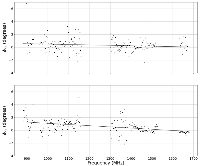
Figure 1: The residual $x-y$ phase angle (degrees) measured from the Stokes $U$ and $V$ spectra of J1331+3030 (3C 286). The top panel shows $\phi_{xy}$ versus frequency for the first run and the bottom for the second run. The lines are a linear fit.

The target sources are distributed over the sky – as far North as +33 and as far South as -84 declination. The transfer of the absolute gain solution from J1939-6342 thus occurs across a large angle on the sky. At GHz frequencies the gain of the system is largely determined by the instrument. The atmosphere plays a minor role. This observing and calibration approach is thus practical for frequencies in the GHz regime. At higher frequencies where the atmosphere has a strong impact on the gains, or at lower frequencies where the ionosphere will strongly affect the $x-y$ phase, this approach may not be practical.

The last step of the calibration is to solve for any remaining $x-y$ phase using the scan on the polarization calibrator J1331+3030 (3C286). A residual error in $x-y$ phase has the effect of rotating flux between $U$ and $V$. For a linear polarized source known to have no circular polarization $V=0$, the $x-y$ phase residual can be measured as

$$\Delta\phi_{xy}=\arctan\biggl{(}\frac{V}{U}\biggr{)}$$ (10)

The residual $x-y$ phase on 3C 286 as a function of frequency for each observing run is shown in Figure  1. The residual phase is small, with a maximum of about 2^∘ at the low end of the band and close to zero at the high end. An $x-y$ phase error of 2^∘ results in a rotation of 0.06% between $U$ and $V$. While small, under the assumption that the Stokes $V$ flux of 3C 286 is actually zero, this final residual $x-y$ phase correction (solid lines in Figure 1) is applied to each source.

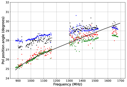
Figure 2: The observed polarization position angle versus frequency for 3C 286 on 19 August 2019 (black dots) and 29 August 2020 (blue dots). The solid black line is the revised model for the polarization position angle of 3C 286 from Hugo & Perley (2023). The red and green dots are the data from 2019 and 2020 with an additional correction to align with the model (see text).

Following calibration, a full Stokes cube for each source was created using the IDIA cube generation pipeline component written by Lennart Heino. The cubes contain Stokes $I$, $Q$, $U$, $V$ images versus frequency in 320 channels, each of width 2.51 MHz. Each channel image is $512\times 512$ pixels with pixel cell size of 1.5^′′. Full Stokes spectra for each source were constructed by extracting the peak flux in the $I$, $Q$, $U$ and $V$ at the location of the peak Stokes $I$ flux density in each channel. The spectral noise for each source was determined by measuring the variance of intensity with frequency for an off-source position in each spectral cube. The median spectral noise per-channel over all sources in $I,\ Q,\ U$ and $V$ is 2.61, 0.30, 0.32 and 0.23 mJy-bm^-1 respectively. Spatial noise per-channel was measured from the standard deviation in a region around the source in each spectral channel.

As a final step, $Q,\ U$ spectra for each source were corrected for ionospheric Faraday rotation using predicted ionospheric Rotation Measures from the World Magnetic Model (WMM)(NCEI Geomagnetic Modeling Team and British Geological Survey., 2019) through the use of the RMExtract software package (Mevius, 2018). RMExtract predicts ionospheric total electron content (TEC) values and rotation measures for a given line of sight and observation time from a geomagnetic field model and Global Navigation Satellite System (GNSS) global ionospheric map.

The observed frequency dependence of the polarization position angle for 3C 286 for each observing run is shown by the black and blue dots in Figure 2. The position angle is similar between runs. The difference between the observed position angle is essentially zero at the high end of the band, increasing to about $0.8^{\circ}$ at 900 MHz.

The solid black line in Figure 2 shows a recent model of the intrinsic polarization position angle of 3C 286 from Hugo & Perley (2023) using MeerKAT observations of the Moon to calibrate absolute position angle. The model agrees with the observed angles above 1500 MHz, but lies below the observations by a few degrees at lower frequencies. The red and green data points in Figure 2 are the observed results from the two observing runs adjusted for a RM of -0.31 rad m^-2 for 19 August 2019 and -0.4 rad m^-2 for 29 August 2020 to align the position angles with the Hugo & Perley (2023) model. The RM adjusted data agree well with the predicted intrinsic values below 1400 MHz, and differ only by about 1^∘ at the high end of the band. These results indicate that residuals to the predicted ionospheric Faraday rotation measures from RMextract are of order -0.4 rad m^-2, resulting in systematic errors in the polarization position angle at 1400 MHz of $\sim$2^∘.

3.1 Residual Instrumental Polarization

The median noise in fractional polarization $Q/I,\ U/I$ and $V/I$ is 0.011, 0.011 and 0.008%, respectively. The limits to the precision of polarization measurements in our observations are higher than this due to residual instrumental polarization. J1939-6342 is assumed to have zero linear and circular polarization. We note that Rayner et al. (2000) have reported a tentative detection of circular polarization of J1939-6342 at 4.8 GHz of $+0.029\pm 0.005\%$, so there may be very low levels of source signal present in $V$.

Since J1939-6342 was observed several times for each observing run, and is the primary polarization leakage calibrator, the residual polarized signal on this sources represents an estimate of the residual error of the fractional polarization. Figure 3 shows the spectrum of polarized signals for J1939-6342 for the two observing runs. The polarization spectra shows signal with structure in frequency and of about 0.1% in linear polarization - about a factor of 10 higher than the RMS noise. The peak-to-peak variation of the signal in $Q/I$ and $U/I$ across the band is similar to the average signal strength. The circularly polarized signal is significantly lower but still present. Maximum peak absolute values in linear polarization are 0.25% and 0.07% in circular polarization. The median and rms values over the band for each Stokes parameter are listed in Table 1. Median linear polarization of J1939-6342 over the band is $\sim 0.15$% for both observing runs. The median circular polarization varies between runs with a maximum value of 0.026%. Conservatively, we set the threshold for polarization detection for linear polarization as band-averaged value greater than 0.2% and median circular polarization greater than 0.08%.

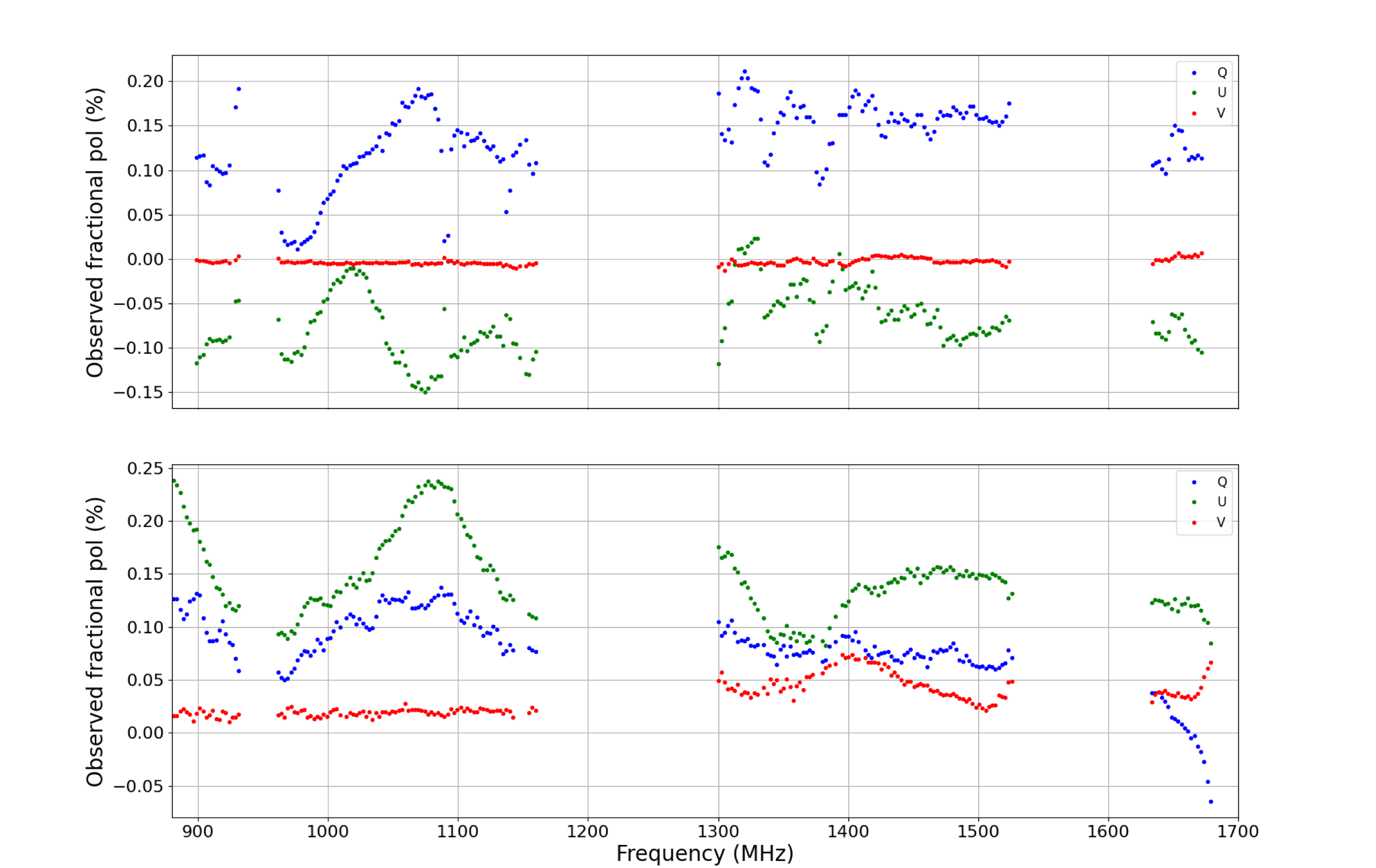
Figure 3: Fractional polarization spectra of J1939-6342 on 19 August 2019 (top) and 29 August 2020 (bottom). For each run, traces are shown for $Q/I$ (blue), $U/I$ (green) and $V/I$ (red).

Date	$Q/I$	$U/I$	$V/I$	$Q/I$	$U/I$	$V/I$
		Median (%)			RMS (%)
19 August 2019	0.082	0.142	0.026	0.033	0.039	0.016
29 August 2020	0.141	-0.075	-0.004	0.044	0.037	0.003

Table 1: Band-averaged polarization of J1939-6342 for the two observing runs.

Residual leakage signals may occur for two main reasons. Firstly, they may stem from instabilities in the bandpass, leading to time variations in the frequency spectrum of the leakage. Secondly, they could arise due to directional variations, either caused by minor changes in the optics concerning antenna orientation or external factors, such as ionospheric effects. These external influences have the potential to impact both the gain phase and the rotation angle of polarization. As noted in section 2, the ionosphere is expected to introduce a polarization dependent phase variation of order a few degrees at L-band.

During the 19 August 2019 run J1939-6342 was observed five times over a time span of about seven hours. For the 20 August 2020 run, J1939-6342 was observed three times over a much shorter span of just under three hours. For the polarization dependent bandpass solution, the solution interval was set to 60 minutes to provide a crude time-dependent solution. For the leakage calibration the solution interval was set to be infinite through the ‘inf’ option of CASA’s polcal() task, to create a single average leakage solution. Any instabilities or the direction dependence from the average value will propagate through as residual errors.

One may not expect ionospheric effects to result in the frequency structure seen in Figure 3. However, one way to test for the impact of the ionosphere is to carry out an observing run at nighttime when the ionosphere is not excited by solar radiance. An indication of the impact of nighttime versus daytime observation is shown in Figure 4. For the second run in August 2020 we observed the strong source J0408-6545 approximately once per hour during the course of the run. The Figure shows the gain amplitude and phase solutions from gaincal as a function of time. These gain solutions were derived after applying the gain solutions from the primary calibrator J1939-6342 and were made with gaintype=‘T’ so the parallel hand correlations are averaged before the solve. If the J1939-6342 solutions were correct for J0408-6545 then the solution gain amplitude solution would be 1.0 and the phase solution would be 0.0. The vertical red line on each plot shows the approximate time of astronomical Sunrise on the date of the observation. It is noteworthy that prior to Sunrise the gain solutions are quite stable and uniformly close to 1.0 in amplitude and 0.0 in phase. The peak-to-peak dispersion is approximately $\pm$0.1% in gain and $\pm$0.3 degrees in phase. About two hours after astronomical Sunrise the dispersion becomes significantly larger, 1-2% in gain and over 1 degree in phase. This strongly suggests that the atmospheric/ionospheric stability is much better during the night (by a factor of several to ten) and thus transfer of gain solutions from the primary calibrator to target sources more precise. This may reduce the level of residual instrumental polarization.

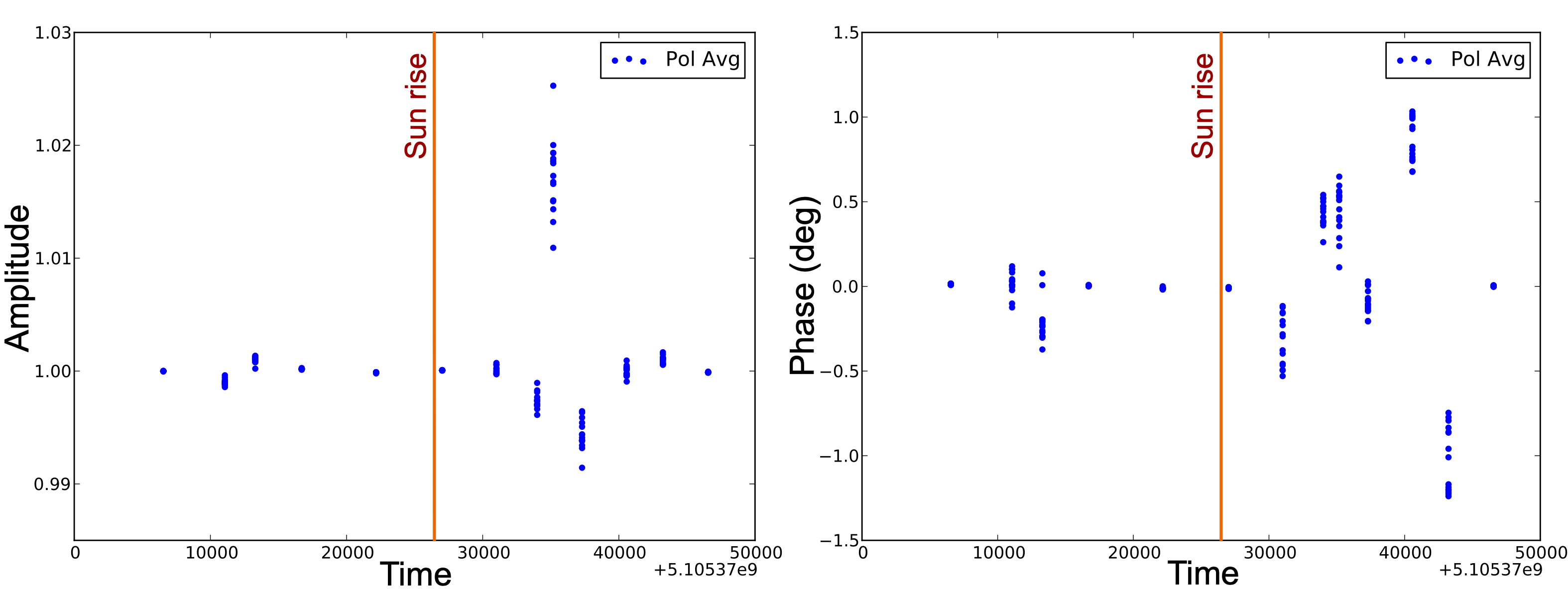
Figure 4: Gaincal solutions for hourly observations of J0408-6545 during the observing run of 29 August 2020. The x-axis shows observation time stamps with solution amplitude and phase given on the y-axes. The left hand panel shows gain amplitude versus time and the right hand panel the gain phase versus time. The vertical red line shows the approximate time of astronomical Sunrise.

4 Results

4.1 Total Intensity Properties

The polarization properties for each source were derived from the spectro-polarimetric data for each source extracted from the $IQUV$ cubes. The in-band total intensity spectra was fit by a power law function of the form

$$I(\nu)=I_{o}\biggl{(}\frac{\nu}{\nu_{o}}\biggr{)}^{\alpha+C\ln{(\nu/\nu_{o})}}.$$ (11)

where $\nu_{o}=1400$ MHz. The curvature term $C$ was included since many of the sources exhibit curved spectra. For example, 12 of the sources exhibit GigaHerz Peak Spectra (GPS) and 7 show evidence of a “valley” spectrum, with a minima of intensity within the band. In total, about 50% of the sources have a significant curvature term.

Figure 5 shows the distribution of in-band spectral and curvature indices for the sources. The median spectral index is $-0.39$. This is flatter than typical of the general source population, which is more typically $-0.7$. This difference can be attributed to the fact that the calibrator sources are selected for brightness and compactness. The optical depth to synchrotron self-absorption is proportional to $(S^{\frac{2}{5}}\theta^{-\frac{4}{5}})$, where $\theta$ is the angular dimension of the source, so synchrotron self-absorption will be more dominant than in the general population.

The colours in the curvature index distribution in Figure 5 show the values for flat spectrum sources ($\alpha>-0.5$) in red and for steep spectrum sources ($\alpha<-0.5)$ in blue. Large values of curvature are predominantly associated with flat spectra.

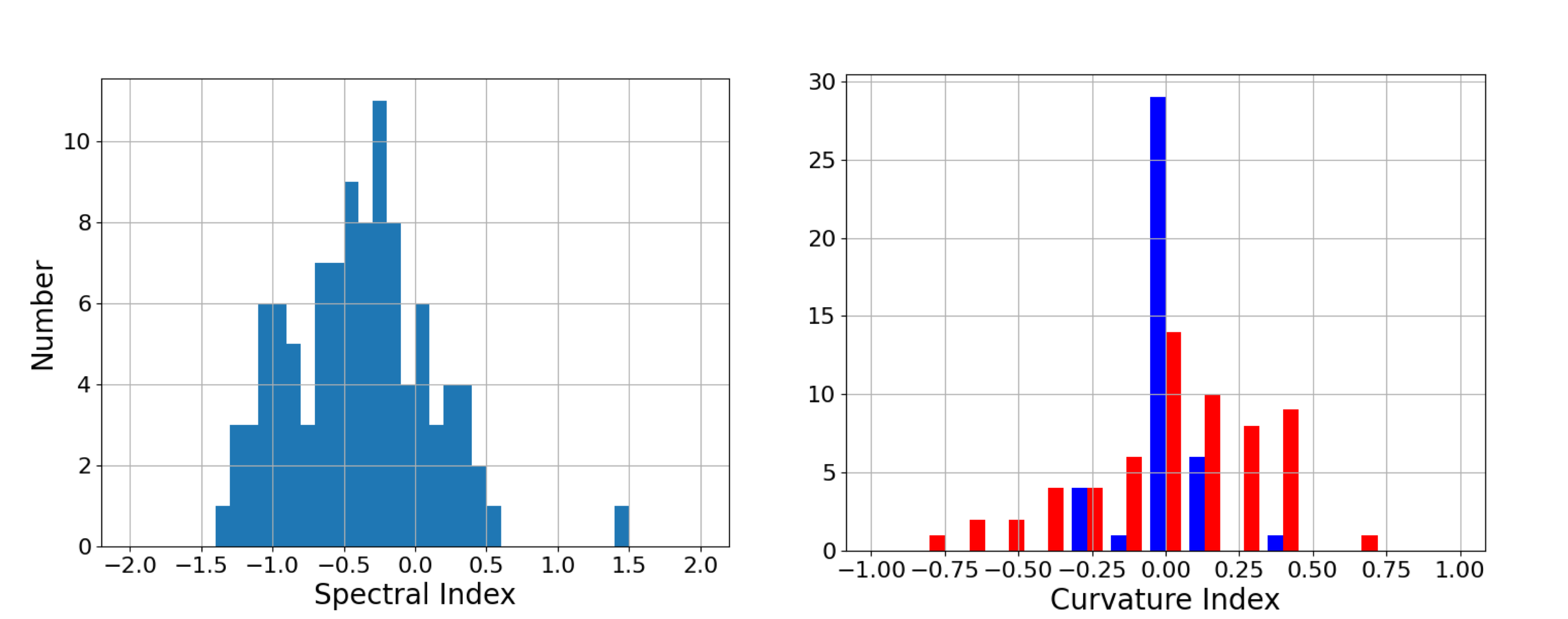
Figure 5: Left panel: The distribution of in-band spectral indices, $\alpha$. Right panel: The distribution of in-band curvature indices. The blue bars are for sources with spectral index $\alpha<-0.5$, and the red for $\alpha>-0.5$.

Figure 6 compares the flux density at 1400 MHz from MeerKAT and NVSS. The dashed line is not a fit. It shows the 1:1 relation. There is a core of sources that fall on the 1:1 line. These sources are apparently flux stable on time scales of 20 years. Two strong sources exhibit high fractional variability, J1924-2914 decreased from 13.4 Jy to 4.9 Jy since the mid 1990’s when the NVSS observation were made. J2253+1608 increased from 12.7 Jy to 16.2 Jy. Several of the fainter sources also show variability. Again, given the compactness criteria for the source selection, the presence of significant variability, particularly over time scales of decades, is not unexpected.

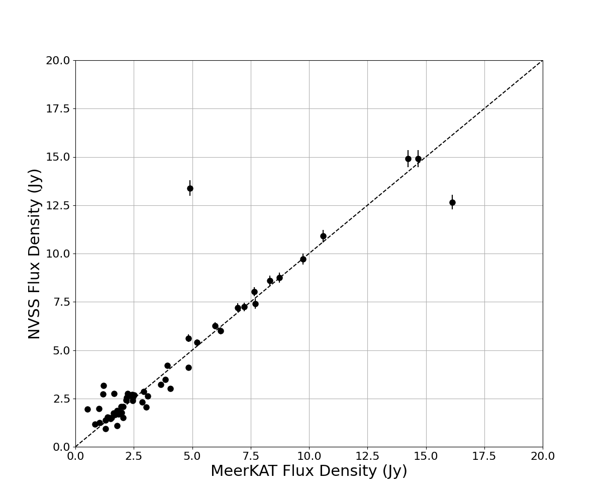
Figure 6: Comparison of the Flux density at 1400 MHz from MeerKAT and NVSS. The dashed line shows the 1:1 relation.

4.2 Linear Polarization Properties of the Calibrators

For each source we derive three measures of the linear polarized signal. A band-averaged fractional linear polarization of the calibrator sources was measured by taking the median polarized intensity $p_{\mathrm{m}ed}$ over all frequency channels. To correct for polarization bias from noise, we measured the standard deviation in $Q$ and $U$ for each channel over an annular box centred on the source position. The per-channel polarized intensity is the ratio of the bias-corrected polarized intensity to the total peak intensity in each channel.

$$p_{i}=\frac{\sqrt{Q_{i}^{2}+U_{i}^{2}-2.3\sigma_{\rm{QU}_{i}}^{2}}}{I_{i}},$$ (12)

where $i$ is the channel number and $\sigma_{\rm{QU}_{i}}$ is the mean of $\sigma_{\rm Q_{i}}$ and $\sigma_{\rm U_{i}}$ for each channel. The bias correction follows the prescription of George et al. (2012). $p_{\mathrm{m}ed}$ is the median of the $p_{i}$ values. The mean frequency of the channels is 1250.2 MHz. The error on $p_{\mathrm{m}ed}$ is calculated as

$$\sigma_{n}=\frac{1}{N}\sum_{i}^{N}\biggl{(}\frac{\sigma_{QU_{i}}}{I_{i}}\biggr{)}\frac{1}{\sqrt{N}}$$ (13)

Here $N$ is the number of channels. This is the error from the noise, and does not include the systematic error.

For comparison to other published results, e.g. the NVSS, we also calculate $p_{\mathrm{1}400}$, the polarized intensity at a frequency of 1400 MHz, as the average polarized intensity over all channels within $\pm$20 MHz of 1400 MHz. The error is given by Equation 13, with $N$ in this case given by the number of channels used for the calculation (typically 15). The linear polarization position angle at 1400 MHz is calculated from the average $Q_{\mathrm{1}400}$ and $U_{\mathrm{1}400}$.

For a third measure of the polarized intensity we calculate a Faraday depth spectrum for each source and record the value of the peak of the dominant component, $p_{\mathrm{m}ax}$. For a Faraday simple spectrum (a single Faraday-thin component) the $p_{\mathrm{m}ax}$ will be similar to $p_{\mathrm{m}ed}$. In the presence of multiple Faraday components $p_{\mathrm{m}ax}$ will underestimate the total polarized intensity of the source.

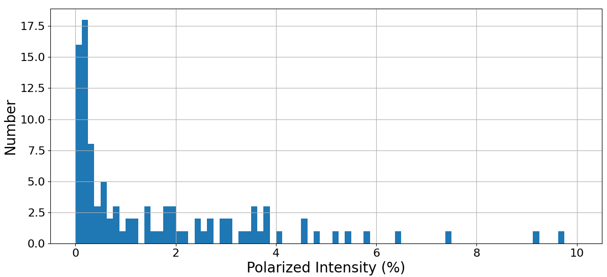
Figure 7: Distribution of linear fractional polarization $p_{\mathrm{m}ed}$ for the calibrator sources.

The distribution of polarized intensity $p_{\mathrm{m}ed}$, for all sources is shown in Figure 7. The distribution is characterized by a broad tail of polarized sources extending up to nearly 10%. The peak that is near zero corresponds to sources with no detectable polarization. We take 0.2% as the minimum detectable polarization. We find that 69 of the calibrators sources are detected in polarization above 0.2%. For the polarized sources we calculated the polarization spectral index $\beta$ as

$$p\propto\lambda^{\beta}$$ (14)

When $\beta<0$ a source is classed as “depolarized”, i.e. the fractional polarization is reduced at longer wavelengths (lower frequencies). For $\beta>0$ a source is “repolarized”, with fractional polarization increasing toward longer wavelengths. Figure 8 shows a plot of the total intensity spectral index $\alpha$ versus $\beta$. The figure shows that for flat spectrum sources ($\alpha>-0.5$) the polarized spectral index $\beta$ is typically flat. Strong depolarization is present predominantly for steep spectrum sources. This result confirms a result first reported in the study of the polarized SEDs of 951 sources from published polarization measurements by Farnes et al. (2014). The distinction in the polarization properties of steep and flat spectrum sources is taken to demonstrate that depolarization properties of sources are due to local source environments.

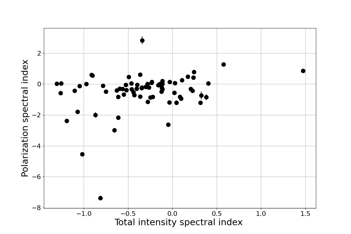
Figure 8: Fractional Polarization spectral index versus total intensity spectral index for 69 source detected in polarization.

4.2.1 Potential Wide-band Polarization Calibrators

Several of the sources show fairly strong fractional polarization. There are 30 sources with $p_{\mathrm{m}ed}>2.0\%$. Many of these have a dominant Faraday Synthesis component at RM of several 10’s of rad m^-2. Calibration sources with high rotation measure complicate polarization calibration over wide-bands at GHz frequencies and below. For the MeerKAT L-band an RM of 10 rad m^-2 produces a rotation of the polarization angle across the band of 48^∘ and rotates flux between Stokes $Q$ and $U$ over the band. The primary polarization calibrators, 3C 286 and 3C 138, have Rotation Measures very close to zero (Perley & Butler, 2013).

Name	$S_{1.4}$	$p_{1400}$	pa1400	RM
	(Jy)	(%)	(∘)	(rad m-2)
J0059+0006	2.45	3.76	67.5	-5.0 $\pm$ 0.1
J0108+0134	3.11	3.88	-86.5	-8.1 $\pm$ 0.1
J1051-2023	1.44	2.30	59.8	-5.6 $\pm$ 0.1
J1239-1023	1.55	2.51	73.8	1.4 $\pm$ 0.1
J1424-4913	8.13	1.84	-10.0	9.6 $\pm$ 0.1
J1512-0906	2.44	3.24	36.8	-11.4 $\pm$ 0.1
J1517-2422	3.03	3.35	35.6	-6.6 $\pm$ 0.1
J1550+0527	2.86	1.77	73.1	-7.4 $\pm$ 0.1
J1923-2104	1.22	2.93	-38.7	8.5 $\pm$ 0.1
J2131-1207	1.97	1.75	-49.9	5.5 $\pm$ 0.1

Table 2: Potential Wide-band polarization calibrators.

Table 2 lists ten objects with fractional polarization greater than 1.5% that have Faraday simple spectra and the Faraday depth of the dominant Faraday Synthesis component less than $\sim$10 rad m^-2. The table lists the J2000 source name, the total intensity flux density at 1400 MHz, the percent polarization and position angle at 1400 MHz, and the Rotation Measure of the dominant Faraday Synthesis component. Figure 9 shows the amplitude Faraday depth spectra for each, showing a single Faraday-thin component. If these objects have stable polarization properties, they would be useful calibrators for broad-band, low-frequency observations.

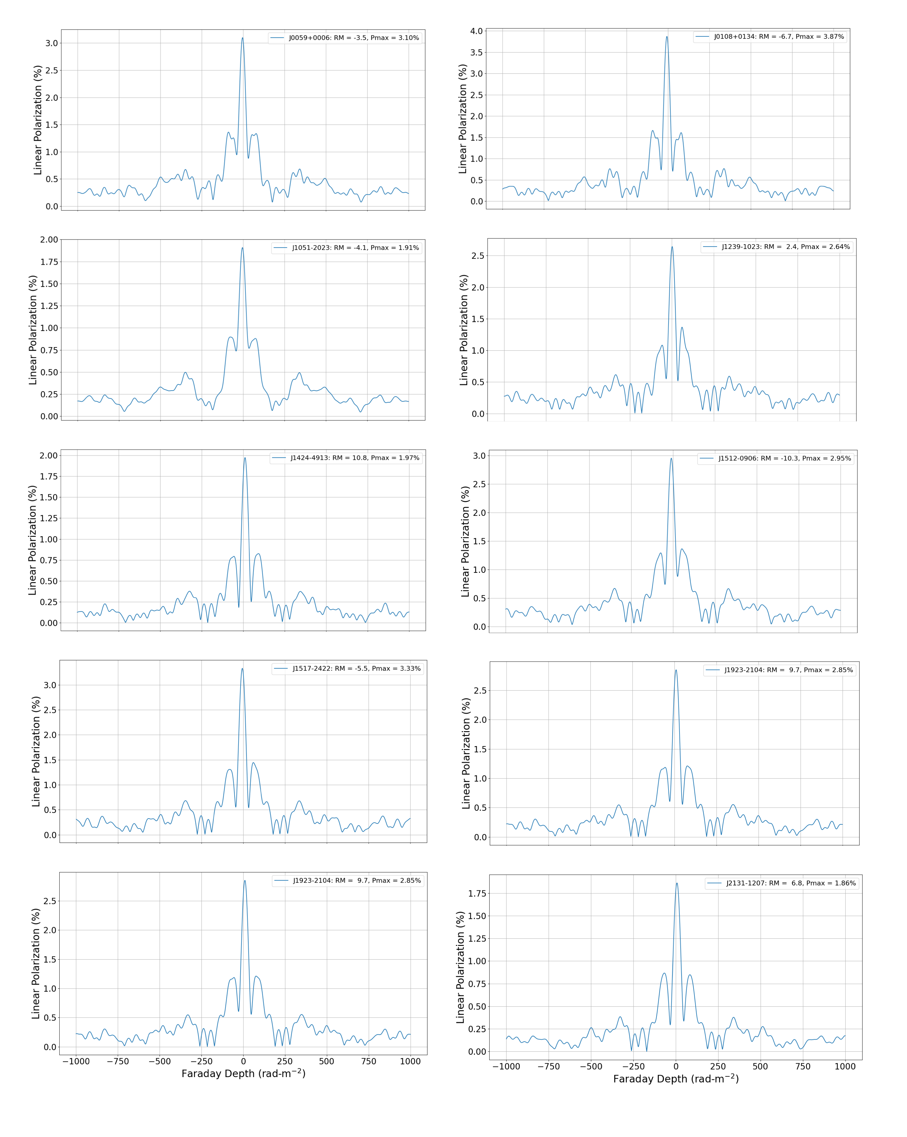
Figure 9: RM synthesis amplitude spectra for the ten sources in Table 2. The spectra are dominated by a single RM component close to zero. The high sidelobes are caused by the missing frequency ranges (see for example Fig. 3.)

4.2.2 Comparison to NVSS and SPASS

Among the MeerKAT 98 calibrator sources, 54 are present in the NVSS RM catalog (Taylor et al., 2009) and 26 are found in the SPASS catalogue (Meyers et al., 2017). Figure 10 shows a comparison of the MeerKAT results to the NVSS and SPASS. The left hand panel of the figure shows the Faraday depth of the dominant component in the RM synthesis spectra of the MeerKAT calibrators compared to the Faraday Rotation Measure observed with the NVSS at 1.4 GHz and the Faraday depth of the dominant component in SPASS at 2.3 GHz. To avoid large errors on the NVSS we include only NVSS sources with percent polarization greater than 1%.

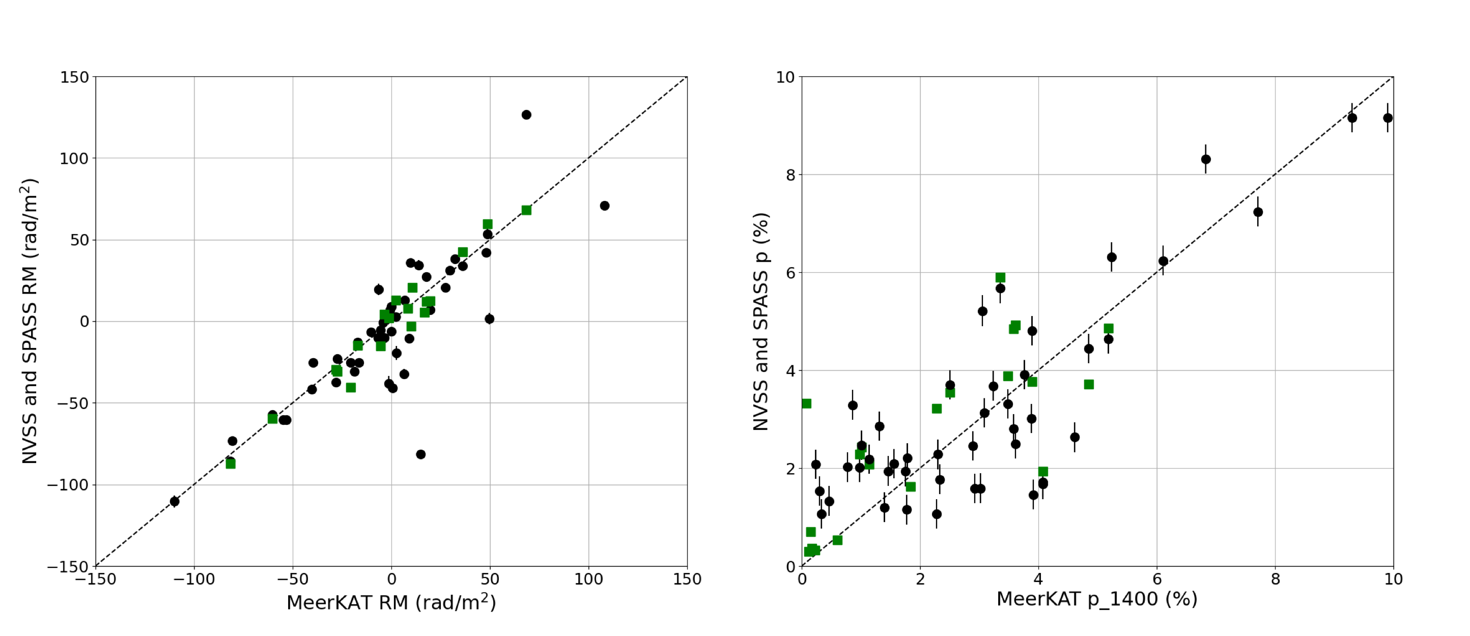
Figure 10: Left panel: Faraday depth of the dominant RM synthesis component for the MeerKAT calibrators compared to the RM from the NVSS (black circles) and dominant Faraday depth component from SPASS (green squares). Right panel: The percent polarization from MeerKAT compared to NVSS (black) and SPASS (green).

The SPASS data show very good agreement to the MeerKAT results. The NVSS also shows generally good agreement, but with a few outliers. The NVSS observations (Condon et al., 1998b) were taken almost 30 years ago. It is not surprising to see some sources vary in RM, particularly given the compact nature of the calibrator source list. We note also that the NVSS RMs were derived from a simple two-point fit to the slope of the position angle with frequency, which will provide a less reliable measure in the presence of Faraday complexity.

The right hand panel of Figure 10 shows MeerKAT percent polarization at 1400 MHz, p₁₄₀₀, compared to the NVSS and the SPASS 2.3 GHz polarization. Error bars on the NVSS polarimetry include the estimated 0.3% systematic error on the NVSS wide-field leakage correction (Condon et al., 1998a). While there is significant scatter in the data, indicating variability in polarization, there is an overall good correlation. The SPASS polarization tends to be higher on average as expected from depolarization. The average SPASS to MeerKAT to depolarization for our sample is

$$D=\frac{\pi_{SP}}{\pi_{MK}}=1.35,$$ (15)

which is similar to values found by Lamee et al. (2016) for 416 sources detected in both the SPASS and NVSS.

4.3 Circular Polarization

The linear feeds of MeerKAT provide the possibility of very precise measurements of circular polarization, as the circular polarized signals appear only in difference of the the cross-hand correlations (Equations 2 and 3) and is contaminated only by the residual polarization leakage and cross-hand phase errors. Circular polarization of extragalactic sources is difficult to measure due to the typically very low fractional polarization. As described in section 3.1, we use the strong unpolarized source J1939-6342 to measure the leakage and the frequency-dependence of the $x$ and $y$ phases independently. The absolute cross-hand ($x-y$) phase difference is calibrated using J1331+3030. After applying the calibration, the residual band-averaged Stokes $V$ signal on J1331+3030 is 0.058%. This value is consistent with the residual $x-y$ phase error discussed in section 3. Assuming no circular polarization for J1331+3030, we can conservatively take this as an estimate of the residual instrumental error on fractional circular polarization. This value is also consistent with the maximum residual circular polarization of J1939-6342 (Fig. 3).

We measure the circular polarized signal from each source by calculating the median amplitude of $v=V/I$ across the band, $v_{\rm med}$. Since circular polarization is a signed quantity, $v_{\rm med}$ may be reduced in the presence of real signal if $V$ changes sign across the band. To mitigate against this effect we also calculate the value of $v$ at 1400 MHz, by fitting the $v$ spectra with Equation 11 and solving for $v_{\rm 1400}$.

As a first step, for each observing run, we compute the median $v(\nu)$ spectrum over all sources. Subsequently, if a source has $v(\nu)<0.2\%$, we subtract the resulting median $v$ spectrum from the source spectrum before measuring $v_{\rm med}$ and $v_{\rm 1400}$. Under the assumption that the median circular polarization of the entire ensemble of sources will stochastically approach zero, this will reduce the effects of any residual instrumental spectrum. Figure 11 shows the distribution of fractional Stokes $V$ for the MeerKAT calibrator sources. The distribution is centrally peaked around zero with several outliers. One source, J0240-2309 is very strongly circularly polarized with $V$ close to 0.4%. The standard deviation of the distribution, measured as 1.486 times the median absolute deviation (MAD), is 0.062%, and the width of the central peak is $\sim$0.2%. We conservatively take 0.07% as the detection threshold for circular polarization.

Figure 11: Distribution of band-averaged fractional Stokes $V$ (%) for the MeerKAT calibrator sources.

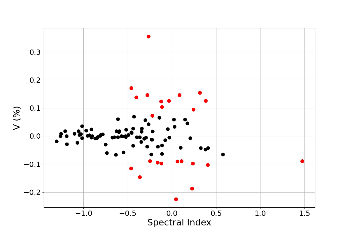
Figure 12: Fractional band-averaged circular polarization (%) versus the MeerKAT spectral index from the Stokes $I$ spectrum. Sources with measured values of $v_{\rm med}$$>0.07$% are shown in red.

Cicular polarization is detected with $v_{\rm med}$ above 0.07% from 24 of the calibrators. Figure 12 plots $v_{\rm med}$ versus the total intensity spectral index, $\alpha$, determined by the fit to the Stokes $I$ spectrum. Source with $V>0.07\%$ are shown in red. Circular polarization is detected in 24% of the sources. It is striking that significant circular polarization is detected only for flat spectrum sources with $\alpha>-0.5$. Steep spectrum sources in the sample do not exhibit circular polarization. This is consistent with the result of high precision circular polarization measurements of 31 radio sources at 5 GHz with the ATCA (Rayner et al., 2000), which also showed circular polarization only for sources with spectral index $\alpha>-0.5$ between wavelengths of 3 cm$-$20 cm.

5 Data Availability

The $IQUV$ image cubes and spectro-polarimetric data for each source are available on the science archive of the South African Radio Astronomy Observatory under DOI https://doi.org/10.48479/sbtr-k883. The site also contains plots of frequency spectra of total intensity, the Stokes $Q$ and $U$ versus $\lambda^{2}$, the Faraday synthesis spectra, and linear and circular polarization spectra for each source.

A summary of the polarization properties of the calibration sources is given in Table A in Appendix A. The columns of the table lists the following properties for each source.

1. The J2000 coordinate source name.

2. The flux density at 1400 MHz ($S_{1.4}$) with error, from a power-law fit to the Stokes $I$ spectrum.

3. The in-band spectral index and error from the spectral fit (Equation 11) to the Stokes $I$ spectrum ($\alpha$). Errors for both the flux density and spectral index are the formal error on the fit parameters from the covariance matrix.

4. The curvature term and error from the spectral fit to the Stokes $I$ spectrum ($\alpha$). Errors are from the covariance matrix.

5. The percent polarized intensity and position angle at 1400 MHz (p₁₄₀₀, pa₁₄₀₀) measured as the average value of polarized intensity and polarization angle over the channels within $\pm$20 MHz of 1400 MHz.

6. The spectral index of polarized intensity ($\beta$) from a power-law fit to the spectrum of polarized intensity (Equation 14). Here also the errors are the formal error on the fit parameter from the covariance matrix.

7. The Faraday depth of the dominant RM synthesis component with error.

8. The amplitude (percent polarization) of the dominant RM synthesis component.

9. The median value fractional Stokes $V$ over the band, $v_{\rm med}$. The error is the standard error on the mean derived from the RMS of the $N$ values over the frequency interval divided by $\sqrt{N}$.

10. The circular polarization at 1400 MHz, $v_{1400}$, with error, from the spectral fit to the $v$ spectrum.

The errors listed in Appendix A include only the random error from the noise of the data. The spectral variance is much smaller than the residual instrumental leakage error, which is estimated as 0.16% in $p$ and 0.05% in $v$. Detection thresholds have been taken as 0.2% for $p$ and 0.07% for $v$. The systematic error on Rotation Measure is 0.3 rad m^-2 and on position angle is 2^∘. The systematic error in flux density is estimated to be 3%, taken as the fractional difference in the derived flux of 3C 286 between the two runs. These systematic uncertainties should be added in quadrature with the errors in the Appendix to derive the total error.

The MeerKAT program of polarization observations of potential calibrators is ongoing. A monitoring program of the ten sources in Table 2 is in progress to assess their potential for this purpose. This MeerKAT program observes the ten sources every $\sim$3 months and has been collecting both L-band and UHF (580 - 1015 MHz corresponding to 544 - 1088 MHz digitized) data since March 2021. These results will be published in a following publication. Similarly, there is an ongoing campaign to characterize the MeerKAT UHF and S-band calibrator sources in full polarization. The S-band campaign is in the early stages of identifying additional suitable MeerKAT S-band calibrator sources whose distribution on the sky covers a larger area than the existing list of S-band calibrators. The UHF campaign, on the other hand, is in the advanced data collection stage with reductions to begin in early 2024.

Appendix A Summary Table of Polarization properties

Table 3: Polarization Properties of MeerKAT Calibrator Sources.

Name	S1.4	$\alpha$	$C$	p1400	pa1400	$\beta$	RM	pmax	vmed	v1400
	$(\mathrm{Jy})$			(%)	$(\mathrm{deg})$		(rad m-2)	(%)	(%)	(%)
J0010-4153	4.562 $\pm$ 0.001	-0.914 $\pm$ 0.002	-0.226 $\pm$ 0.007	0.12 $\pm$ 0.002	-67.4 $\pm$ 0.8	-0.24 $\pm$ 0.18	-2.8 $\pm$ 0.2	0.14	0.024 $\pm$ 0.002	0.020 $\pm$ 0.002
J0022+0014	2.913 $\pm$ 0.001	-0.634 $\pm$ 0.003	-0.250 $\pm$ 0.008	0.09 $\pm$ 0.002	-18.3 $\pm$ 1.7	-1.53 $\pm$ 0.23	0.5 $\pm$ 0.2	0.13	-0.066 $\pm$ 0.001	-0.067 $\pm$ 0.002
J0024-4202	2.914 $\pm$ 0.001	0.407 $\pm$ 0.003	-0.830 $\pm$ 0.012	0.09 $\pm$ 0.002	-11.3 $\pm$ 1.1	-0.36 $\pm$ 0.20	3.0 $\pm$ 0.2	0.13	-0.043 $\pm$ 0.002	-0.056 $\pm$ 0.002
J0025-2602	8.734 $\pm$ 0.002	-0.738 $\pm$ 0.002	-0.017 $\pm$ 0.006	0.17 $\pm$ 0.001	65.7 $\pm$ 1.2	0.31 $\pm$ 0.13	-5.2 $\pm$ 0.1	0.18	-0.060 $\pm$ 0.003	-0.062 $\pm$ 0.004
J0059+0006	2.447 $\pm$ 0.001	-0.548 $\pm$ 0.003	0.041 $\pm$ 0.008	3.76 $\pm$ 0.003	67.5 $\pm$ 0.6	-0.68 $\pm$ 0.03	-5.0 $\pm$ 0.1	3.10	-0.053 $\pm$ 0.001	-0.046 $\pm$ 0.006
J0108+0134	3.106 $\pm$ 0.001	-0.232 $\pm$ 0.004	0.144 $\pm$ 0.011	3.88 $\pm$ 0.003	-86.5 $\pm$ 0.2	0.13 $\pm$ 0.01	-8.1 $\pm$ 0.1	3.87	-0.007 $\pm$ 0.001	0.112 $\pm$ 0.020
J0137+3309	16.096 $\pm$ 0.004	-0.869 $\pm$ 0.002	0.067 $\pm$ 0.005	0.64 $\pm$ 0.003	-43.2 $\pm$ 0.6	-2.01 $\pm$ 0.17	-56.8 $\pm$ 0.1	0.49	-0.009 $\pm$ 0.001	-0.004 $\pm$ 0.002
J0155-4048	2.161 $\pm$ 0.001	-0.458 $\pm$ 0.003	-0.010 $\pm$ 0.008	0.07 $\pm$ 0.003	22.7 $\pm$ 2.3	1.72 $\pm$ 0.13	-1.6 $\pm$ 0.3	0.08	0.011 $\pm$ 0.001	0.012 $\pm$ 0.002
J0203-4349	2.725 $\pm$ 0.001	-0.815 $\pm$ 0.003	0.036 $\pm$ 0.008	0.91 $\pm$ 0.002	-62.7 $\pm$ 0.3	-7.37 $\pm$ 0.14	-9.8 $\pm$ 0.1	0.49	0.001 $\pm$ 0.001	-0.000 $\pm$ 0.001
J0210-5101	3.385 $\pm$ 0.001	0.206 $\pm$ 0.003	0.276 $\pm$ 0.011	1.24 $\pm$ 0.002	23.4 $\pm$ 0.2	-0.31 $\pm$ 0.02	13.0 $\pm$ 0.1	1.12	-0.005 $\pm$ 0.001	-0.053 $\pm$ 0.005
J0238+1636	0.524 $\pm$ 0.001	-0.114 $\pm$ 0.012	0.466 $\pm$ 0.035	0.77 $\pm$ 0.013	81.9 $\pm$ 0.9	0.20 $\pm$ 0.10	46.6 $\pm$ 0.1	0.72	-0.062 $\pm$ 0.003	-0.113 $\pm$ 0.007
J0240-2309	5.978 $\pm$ 0.002	-0.266 $\pm$ 0.003	-0.401 $\pm$ 0.008	0.98 $\pm$ 0.002	-49.2 $\pm$ 0.1	-0.21 $\pm$ 0.05	8.5 $\pm$ 0.1	0.98	0.353 $\pm$ 0.001	0.307 $\pm$ 0.002
J0252-7104	5.810 $\pm$ 0.001	-0.971 $\pm$ 0.002	0.004 $\pm$ 0.005	0.18 $\pm$ 0.001	-42.8 $\pm$ 0.2	0.01 $\pm$ 0.10	0.7 $\pm$ 0.2	0.23	0.018 $\pm$ 0.001	0.019 $\pm$ 0.001
J0303-6211	3.198 $\pm$ 0.001	-0.112 $\pm$ 0.004	-0.066 $\pm$ 0.011	4.71 $\pm$ 0.002	39.2 $\pm$ 0.5	-0.34 $\pm$ 0.01	47.9 $\pm$ 0.1	4.43	-0.037 $\pm$ 0.001	-0.032 $\pm$ 0.006
J0318+1628	7.653 $\pm$ 0.002	-0.602 $\pm$ 0.002	-0.260 $\pm$ 0.007	0.03 $\pm$ 0.002	-15.8 $\pm$ 10.4	-2.22 $\pm$ 0.34	3.5 $\pm$ 0.4	0.05	0.015 $\pm$ 0.001	0.001 $\pm$ 0.001
J0323+0534	2.764 $\pm$ 0.001	-0.911 $\pm$ 0.004	0.029 $\pm$ 0.010	0.26 $\pm$ 0.003	-78.6 $\pm$ 0.3	0.59 $\pm$ 0.12	0.9 $\pm$ 0.1	0.33	-0.006 $\pm$ 0.001	-0.007 $\pm$ 0.002
J0329+2756	1.397 $\pm$ 0.001	-0.365 $\pm$ 0.004	-0.104 $\pm$ 0.012	0.16 $\pm$ 0.005	-10.7 $\pm$ 1.2	-0.82 $\pm$ 0.14	0.9 $\pm$ 0.2	0.21	-0.148 $\pm$ 0.001	-0.133 $\pm$ 0.002
J0403+2600	1.295 $\pm$ 0.001	-0.033 $\pm$ 0.004	-0.248 $\pm$ 0.012	3.05 $\pm$ 0.005	68.6 $\pm$ 0.6	-1.19 $\pm$ 0.01	48.4 $\pm$ 0.1	2.62	0.131 $\pm$ 0.002	0.111 $\pm$ 0.008
J0405-1308	3.936 $\pm$ 0.002	-0.494 $\pm$ 0.004	0.140 $\pm$ 0.011	1.14 $\pm$ 0.002	24.4 $\pm$ 0.3	0.46 $\pm$ 0.04	18.1 $\pm$ 0.1	1.18	0.006 $\pm$ 0.001	0.004 $\pm$ 0.002
J0408-6545	15.207 $\pm$ 0.002	-1.210 $\pm$ 0.001	-0.033 $\pm$ 0.003	0.01 $\pm$ 0.000	-72.7 $\pm$ 0.8	1.05 $\pm$ 0.10	-0.5 $\pm$ 0.3	0.02	0.018 $\pm$ 0.001	0.022 $\pm$ 0.001
J0409-1757	2.203 $\pm$ 0.001	-0.841 $\pm$ 0.004	0.047 $\pm$ 0.012	0.15 $\pm$ 0.003	-42.3 $\pm$ 1.0	0.63 $\pm$ 0.10	3.6 $\pm$ 0.1	0.20	-0.004 $\pm$ 0.001	-0.007 $\pm$ 0.002
J0420-6223	3.323 $\pm$ 0.001	-1.030 $\pm$ 0.003	0.069 $\pm$ 0.009	0.12 $\pm$ 0.002	58.3 $\pm$ 0.4	0.00 $\pm$ 0.10	0.9 $\pm$ 0.2	0.16	0.007 $\pm$ 0.001	0.009 $\pm$ 0.002
J0423-0120	1.187 $\pm$ 0.001	0.029 $\pm$ 0.005	0.417 $\pm$ 0.014	4.07 $\pm$ 0.005	31.9 $\pm$ 0.3	0.06 $\pm$ 0.01	-22.1 $\pm$ 0.1	3.98	0.031 $\pm$ 0.002	0.026 $\pm$ 0.008
J0440-4333	3.591 $\pm$ 0.002	-0.751 $\pm$ 0.004	0.043 $\pm$ 0.010	0.60 $\pm$ 0.002	-83.9 $\pm$ 0.2	-0.48 $\pm$ 0.02	6.8 $\pm$ 0.1	0.57	-0.031 $\pm$ 0.001	-0.019 $\pm$ 0.002
J0447-2203	2.028 $\pm$ 0.001	-1.047 $\pm$ 0.003	-0.065 $\pm$ 0.009	0.23 $\pm$ 0.003	-31.8 $\pm$ 0.5	-0.13 $\pm$ 0.10	0.3 $\pm$ 0.1	0.28	0.003 $\pm$ 0.001	0.000 $\pm$ 0.001
J0453-2807	2.192 $\pm$ 0.001	-0.340 $\pm$ 0.004	0.007 $\pm$ 0.012	0.59 $\pm$ 0.003	9.8 $\pm$ 1.6	2.83 $\pm$ 0.26	18.0 $\pm$ 0.1	1.73	0.026 $\pm$ 0.001	0.039 $\pm$ 0.006
J0503+0203	2.233 $\pm$ 0.001	0.148 $\pm$ 0.004	-0.356 $\pm$ 0.014	0.04 $\pm$ 0.003	34.5 $\pm$ 1.8	1.51 $\pm$ 0.14	0.0 $\pm$ 0.5	0.06	0.059 $\pm$ 0.001	0.072 $\pm$ 0.002
J0521+1638	8.320 $\pm$ 0.002	-0.613 $\pm$ 0.002	0.083 $\pm$ 0.005	7.71 $\pm$ 0.002	-15.1 $\pm$ 0.2	-0.83 $\pm$ 0.01	-2.4 $\pm$ 0.1	7.03	0.049 $\pm$ 0.001	0.023 $\pm$ 0.007
J0534+1927	6.739 $\pm$ 0.002	-0.849 $\pm$ 0.002	0.022 $\pm$ 0.006	0.02 $\pm$ 0.001	-10.4 $\pm$ 11.1	-2.06 $\pm$ 0.29	5.2 $\pm$ 0.3	0.05	-0.007 $\pm$ 0.001	-0.006 $\pm$ 0.001
J0538-4405	2.142 $\pm$ 0.001	-0.226 $\pm$ 0.004	0.384 $\pm$ 0.011	0.07 $\pm$ 0.002	63.5 $\pm$ 1.1	3.25 $\pm$ 0.14	47.2 $\pm$ 0.2	0.17	-0.013 $\pm$ 0.001	-0.004 $\pm$ 0.002
J0609-1542	1.663 $\pm$ 0.001	-0.462 $\pm$ 0.006	0.356 $\pm$ 0.016	2.28 $\pm$ 0.003	2.1 $\pm$ 0.9	0.05 $\pm$ 0.03	66.8 $\pm$ 0.1	2.45	-0.117 $\pm$ 0.001	-0.116 $\pm$ 0.003
J0616-3456	2.902 $\pm$ 0.001	-0.571 $\pm$ 0.003	0.042 $\pm$ 0.008	0.13 $\pm$ 0.002	84.8 $\pm$ 0.4	0.22 $\pm$ 0.09	-0.2 $\pm$ 0.2	0.16	-0.001 $\pm$ 0.001	-0.018 $\pm$ 0.003
J0632+1022	2.441 $\pm$ 0.001	-0.526 $\pm$ 0.003	-0.326 $\pm$ 0.008	0.24 $\pm$ 0.002	30.6 $\pm$ 0.9	-0.06 $\pm$ 0.10	1.3 $\pm$ 0.1	0.27	0.001 $\pm$ 0.001	0.032 $\pm$ 0.003
J0725-0054	11.809 $\pm$ 0.004	0.228 $\pm$ 0.003	-0.374 $\pm$ 0.009	2.52 $\pm$ 0.003	-19.5 $\pm$ 0.6	-0.43 $\pm$ 0.01	47.6 $\pm$ 0.1	2.39	-0.187 $\pm$ 0.001	-0.204 $\pm$ 0.003
J0730-1141	2.246 $\pm$ 0.002	0.576 $\pm$ 0.008	0.366 $\pm$ 0.026	0.98 $\pm$ 0.003	-79.6 $\pm$ 1.7	1.27 $\pm$ 0.10	106.7 $\pm$ 0.1	1.49	-0.069 $\pm$ 0.001	-0.064 $\pm$ 0.002
J0735-1735	2.598 $\pm$ 0.001	-0.162 $\pm$ 0.004	0.039 $\pm$ 0.013	0.06 $\pm$ 0.002	43.1 $\pm$ 2.3	-1.40 $\pm$ 0.20	-1.5 $\pm$ 0.4	0.07	-0.095 $\pm$ 0.001	-0.088 $\pm$ 0.001
J0739+0137	1.014 $\pm$ 0.001	0.243 $\pm$ 0.004	0.386 $\pm$ 0.013	5.24 $\pm$ 0.006	-52.2 $\pm$ 18.9	0.79 $\pm$ 0.01	26.3 $\pm$ 0.1	5.81	0.092 $\pm$ 0.001	0.072 $\pm$ 0.005
J0745+1011	3.254 $\pm$ 0.002	0.382 $\pm$ 0.004	-0.484 $\pm$ 0.015	0.22 $\pm$ 0.004	40.3 $\pm$ 0.4	-0.85 $\pm$ 0.19	2.0 $\pm$ 0.2	0.27	0.126 $\pm$ 0.001	0.129 $\pm$ 0.001
J0825-5010	6.309 $\pm$ 0.002	0.377 $\pm$ 0.002	-0.576 $\pm$ 0.008	0.23 $\pm$ 0.001	53.9 $\pm$ 2.2	1.30 $\pm$ 0.19	-0.2 $\pm$ 0.1	0.12	-0.047 $\pm$ 0.001	-0.071 $\pm$ 0.001
J0828-3731	2.090 $\pm$ 0.002	-0.282 $\pm$ 0.007	-0.075 $\pm$ 0.022	0.35 $\pm$ 0.003	63.3 $\pm$ 17.3	0.01 $\pm$ 0.09	0.0 $\pm$ 0.1	0.45	-0.037 $\pm$ 0.001	-0.025 $\pm$ 0.002
J0842+1835	1.037 $\pm$ 0.001	-0.278 $\pm$ 0.007	0.098 $\pm$ 0.020	3.09 $\pm$ 0.006	7.9 $\pm$ 0.3	-1.15 $\pm$ 0.03	31.0 $\pm$ 0.1	2.60	0.147 $\pm$ 0.001	0.119 $\pm$ 0.003
J0854+2006	2.048 $\pm$ 0.001	0.084 $\pm$ 0.003	-0.021 $\pm$ 0.009	6.83 $\pm$ 0.005	24.0 $\pm$ 0.3	-0.82 $\pm$ 0.01	28.8 $\pm$ 0.1	6.05	0.150 $\pm$ 0.001	0.179 $\pm$ 0.009
J0906-6829	1.817 $\pm$ 0.001	-1.103 $\pm$ 0.003	0.012 $\pm$ 0.007	2.27 $\pm$ 0.003	-34.6 $\pm$ 0.5	-0.44 $\pm$ 0.03	-49.8 $\pm$ 0.1	2.06	0.008 $\pm$ 0.001	0.008 $\pm$ 0.002
J1008+0730	6.526 $\pm$ 0.001	-0.902 $\pm$ 0.002	0.061 $\pm$ 0.005	0.22 $\pm$ 0.002	-11.9 $\pm$ 0.2	0.56 $\pm$ 0.07	-0.8 $\pm$ 0.1	0.30	-0.000 $\pm$ 0.001	-0.000 $\pm$ 0.001
J1051-2023	1.442 $\pm$ 0.001	-1.072 $\pm$ 0.003	0.009 $\pm$ 0.009	2.30 $\pm$ 0.004	59.8 $\pm$ 0.1	-1.80 $\pm$ 0.03	-5.6 $\pm$ 0.1	1.91	-0.021 $\pm$ 0.001	-0.024 $\pm$ 0.003
J1058+0133	3.665 $\pm$ 0.001	-0.222 $\pm$ 0.003	0.118 $\pm$ 0.008	4.07 $\pm$ 0.003	-17.9 $\pm$ 0.5	-0.83 $\pm$ 0.02	-41.0 $\pm$ 0.1	3.65	0.074 $\pm$ 0.001	0.082 $\pm$ 0.007
J1120-2508	1.640 $\pm$ 0.001	-0.613 $\pm$ 0.007	-0.053 $\pm$ 0.023	1.46 $\pm$ 0.004	-37.2 $\pm$ 0.2	-2.18 $\pm$ 0.05	8.0 $\pm$ 0.1	1.14	-0.005 $\pm$ 0.001	-0.006 $\pm$ 0.002
J1130-1449	4.842 $\pm$ 0.003	-0.250 $\pm$ 0.006	-0.061 $\pm$ 0.018	4.85 $\pm$ 0.003	66.3 $\pm$ 0.5	-0.87 $\pm$ 0.02	35.2 $\pm$ 0.1	4.27	-0.093 $\pm$ 0.001	-0.095 $\pm$ 0.005
J1154-3505	6.088 $\pm$ 0.004	-0.523 $\pm$ 0.006	-0.048 $\pm$ 0.019	0.16 $\pm$ 0.004	43.8 $\pm$ 1.2	1.70 $\pm$ 0.16	-5.9 $\pm$ 0.2	0.19	-0.004 $\pm$ 0.001	-0.003 $\pm$ 0.002
J1215-1731	1.695 $\pm$ 0.001	-0.345 $\pm$ 0.007	0.195 $\pm$ 0.021	2.01 $\pm$ 0.004	6.9 $\pm$ 0.2	-0.22 $\pm$ 0.02	-15.7 $\pm$ 0.1	1.88	0.015 $\pm$ 0.001	0.024 $\pm$ 0.003
J1239-1023	1.558 $\pm$ 0.001	-0.112 $\pm$ 0.007	-0.163 $\pm$ 0.023	2.51 $\pm$ 0.004	73.8 $\pm$ 0.2	-0.00 $\pm$ 0.05	1.4 $\pm$ 0.1	2.64	0.106 $\pm$ 0.001	0.099 $\pm$ 0.003
J1246-2547	0.845 $\pm$ 0.001	0.173 $\pm$ 0.007	0.678 $\pm$ 0.025	3.48 $\pm$ 0.007	-30.6 $\pm$ 0.4	0.48 $\pm$ 0.02	-29.2 $\pm$ 0.1	3.67	0.047 $\pm$ 0.002	0.051 $\pm$ 0.005
J1256-0547	9.734 $\pm$ 0.013	-0.403 $\pm$ 0.012	0.329 $\pm$ 0.036	3.61 $\pm$ 0.004	-44.7 $\pm$ 0.2	-0.30 $\pm$ 0.04	16.9 $\pm$ 0.1	3.43	0.136 $\pm$ 0.001	0.156 $\pm$ 0.003
J1311-2216	4.834 $\pm$ 0.005	-1.190 $\pm$ 0.010	0.338 $\pm$ 0.028	0.05 $\pm$ 0.004	13.3 $\pm$ 7.4	-0.64 $\pm$ 0.33	-13.8 $\pm$ 1.1	0.04	-0.029 $\pm$ 0.001	-0.027 $\pm$ 0.002
J1318-4620	2.205 $\pm$ 0.002	-0.935 $\pm$ 0.008	-0.001 $\pm$ 0.022	0.04 $\pm$ 0.004	-11.5 $\pm$ 16.1	0.17 $\pm$ 0.25	0.5 $\pm$ 0.5	0.10	0.003 $\pm$ 0.001	0.001 $\pm$ 0.001
J1323-4452	3.026 $\pm$ 0.003	-0.808 $\pm$ 0.008	-0.004 $\pm$ 0.025	0.11 $\pm$ 0.004	-2.6 $\pm$ 2.2	-0.29 $\pm$ 0.30	-0.3 $\pm$ 1.3	0.04	0.005 $\pm$ 0.001	0.000 $\pm$ 0.001
J1331+3030	14.673 $\pm$ 0.003	-0.630 $\pm$ 0.002	0.001 $\pm$ 0.005	9.90 $\pm$ 0.003	29.2 $\pm$ 0.1	-0.42 $\pm$ 0.01	-0.3 $\pm$ 0.1	9.39	0.016 $\pm$ 0.001	0.029 $\pm$ 0.012
J1337-1257	2.509 $\pm$ 0.002	0.315 $\pm$ 0.007	0.404 $\pm$ 0.023	1.01 $\pm$ 0.004	-1.6 $\pm$ 0.3	-1.20 $\pm$ 0.05	-18.3 $\pm$ 0.1	0.81	0.154 $\pm$ 0.001	0.137 $\pm$ 0.001
J1347+1217	5.203 $\pm$ 0.004	-0.459 $\pm$ 0.006	0.113 $\pm$ 0.018	0.04 $\pm$ 0.004	55.2 $\pm$ 3.5	-0.78 $\pm$ 0.24	7.0 $\pm$ 0.9	0.04	0.014 $\pm$ 0.001	0.019 $\pm$ 0.001
J1424-4913	8.123 $\pm$ 0.004	-0.366 $\pm$ 0.005	0.059 $\pm$ 0.015	1.84 $\pm$ 0.003	-10.0 $\pm$ 0.2	0.61 $\pm$ 0.01	9.6 $\pm$ 0.1	1.97	-0.004 $\pm$ 0.001	-0.001 $\pm$ 0.001
J1427-4206	4.465 $\pm$ 0.004	-0.049 $\pm$ 0.007	-0.014 $\pm$ 0.024	2.00 $\pm$ 0.003	-51.6 $\pm$ 0.4	-2.62 $\pm$ 0.06	-40.8 $\pm$ 0.1	1.54	0.025 $\pm$ 0.001	0.031 $\pm$ 0.002
J1445+0958	2.177 $\pm$ 0.002	-0.461 $\pm$ 0.007	-0.307 $\pm$ 0.021	0.86 $\pm$ 0.004	-80.7 $\pm$ 0.3	-0.33 $\pm$ 0.04	13.1 $\pm$ 0.1	0.78	0.172 $\pm$ 0.001	0.182 $\pm$ 0.002
J1501-3918	2.805 $\pm$ 0.003	-0.675 $\pm$ 0.008	0.011 $\pm$ 0.024	0.19 $\pm$ 0.003	12.9 $\pm$ 0.7	0.21 $\pm$ 0.09	-0.4 $\pm$ 0.2	0.21	-0.005 $\pm$ 0.001	-0.004 $\pm$ 0.001
J1512-0906	2.434 $\pm$ 0.002	0.021 $\pm$ 0.006	0.205 $\pm$ 0.020	3.24 $\pm$ 0.003	36.8 $\pm$ 0.1	-0.57 $\pm$ 0.01	-11.4 $\pm$ 0.1	2.95	0.059 $\pm$ 0.001	0.067 $\pm$ 0.001
J1517-2422	3.030 $\pm$ 0.002	-0.031 $\pm$ 0.006	-0.084 $\pm$ 0.019	3.35 $\pm$ 0.003	35.6 $\pm$ 0.2	0.13 $\pm$ 0.03	-6.6 $\pm$ 0.1	3.33	-0.005 $\pm$ 0.001	-0.005 $\pm$ 0.003
J1550+0527	2.864 $\pm$ 0.002	-0.160 $\pm$ 0.006	0.008 $\pm$ 0.020	1.77 $\pm$ 0.004	73.1 $\pm$ 0.2	-0.07 $\pm$ 0.01	-7.4 $\pm$ 0.1	1.68	-0.036 $\pm$ 0.001	-0.031 $\pm$ 0.002
J1605-1734	1.375 $\pm$ 0.001	-1.193 $\pm$ 0.009	0.028 $\pm$ 0.026	2.33 $\pm$ 0.004	-54.5 $\pm$ 1.2	-2.38 $\pm$ 0.05	-111.3 $\pm$ 0.1	1.93	0.000 $\pm$ 0.001	-0.000 $\pm$ 0.001
J1609+2641	4.650 $\pm$ 0.003	-0.430 $\pm$ 0.006	-0.446 $\pm$ 0.019	0.24 $\pm$ 0.005	-52.3 $\pm$ 0.7	-0.71 $\pm$ 0.14	3.8 $\pm$ 0.2	0.24	0.069 $\pm$ 0.001	0.065 $\pm$ 0.002
J1619-8418	1.513 $\pm$ 0.002	-1.057 $\pm$ 0.010	0.034 $\pm$ 0.028	0.04 $\pm$ 0.005	40.7 $\pm$ 14.5	-0.13 $\pm$ 0.18	1.9 $\pm$ 0.7	0.05	0.018 $\pm$ 0.001	0.014 $\pm$ 0.003
J1726-5529	5.237 $\pm$ 0.003	-0.078 $\pm$ 0.005	-0.331 $\pm$ 0.018	0.13 $\pm$ 0.003	-71.2 $\pm$ 0.6	0.43 $\pm$ 0.13	-1.1 $\pm$ 0.2	0.18	-0.014 $\pm$ 0.001	-0.012 $\pm$ 0.001
J1733-1304	6.217 $\pm$ 0.004	-0.303 $\pm$ 0.006	-0.017 $\pm$ 0.019	3.58 $\pm$ 0.003	-85.1 $\pm$ 0.9	-0.18 $\pm$ 0.03	-61.5 $\pm$ 0.1	3.65	0.057 $\pm$ 0.001	0.055 $\pm$ 0.002
J1744-5144	6.932 $\pm$ 0.003	-0.294 $\pm$ 0.004	-0.131 $\pm$ 0.013	0.10 $\pm$ 0.003	-14.4 $\pm$ 1.6	-1.18 $\pm$ 0.21	-11.3 $\pm$ 0.3	0.07	-0.005 $\pm$ 0.001	-0.006 $\pm$ 0.001
J1830-3602	7.236 $\pm$ 0.005	-1.305 $\pm$ 0.006	-0.075 $\pm$ 0.018	0.30 $\pm$ 0.002	-86.1 $\pm$ 0.6	0.02 $\pm$ 0.13	-0.8 $\pm$ 0.1	0.36	-0.018 $\pm$ 0.001	-0.015 $\pm$ 0.001
J1833-2103	10.610 $\pm$ 0.006	0.063 $\pm$ 0.005	0.311 $\pm$ 0.016	0.14 $\pm$ 0.003	-30.4 $\pm$ 1.6	-1.29 $\pm$ 0.15	-9.6 $\pm$ 0.3	0.11	-0.089 $\pm$ 0.001	-0.100 $\pm$ 0.002
J1859-6615	1.601 $\pm$ 0.002	-0.956 $\pm$ 0.010	0.074 $\pm$ 0.030	0.16 $\pm$ 0.004	3.3 $\pm$ 0.8	-2.35 $\pm$ 0.19	6.8 $\pm$ 0.3	0.08	0.001 $\pm$ 0.001	0.001 $\pm$ 0.002
J1911-2006	2.289 $\pm$ 0.002	0.235 $\pm$ 0.006	-0.127 $\pm$ 0.021	1.79 $\pm$ 0.003	-84.0 $\pm$ 1.0	0.43 $\pm$ 0.02	-81.7 $\pm$ 0.1	1.94	-0.099 $\pm$ 0.001	-0.100 $\pm$ 0.001
J1923-2104	1.213 $\pm$ 0.001	-0.144 $\pm$ 0.008	0.128 $\pm$ 0.025	2.93 $\pm$ 0.004	-38.7 $\pm$ 0.2	-0.00 $\pm$ 0.03	8.5 $\pm$ 0.1	2.85	0.065 $\pm$ 0.001	0.075 $\pm$ 0.002
J1924-2914	4.908 $\pm$ 0.003	-0.349 $\pm$ 0.005	0.371 $\pm$ 0.017	1.31 $\pm$ 0.003	-2.3 $\pm$ 0.2	-0.26 $\pm$ 0.02	-19.9 $\pm$ 0.1	1.21	-0.021 $\pm$ 0.001	-0.005 $\pm$ 0.002
J1939-6342	14.465 $\pm$ 0.003	-0.266 $\pm$ 0.002	-0.673 $\pm$ 0.005	0.15 $\pm$ 0.001	28.1 $\pm$ 0.6	0.58 $\pm$ 0.08	-1.1 $\pm$ 0.1	0.17	0.043 $\pm$ 0.001	0.057 $\pm$ 0.001
J1939-6342	14.702 $\pm$ 0.005	-0.220 $\pm$ 0.003	-0.661 $\pm$ 0.010	0.16 $\pm$ 0.002	-6.1 $\pm$ 1.5	-0.55 $\pm$ 0.10	-2.7 $\pm$ 0.2	0.15	0.016 $\pm$ 0.001	0.032 $\pm$ 0.001
J1951-2737	1.297 $\pm$ 0.002	-1.018 $\pm$ 0.011	0.014 $\pm$ 0.032	1.40 $\pm$ 0.005	-85.9 $\pm$ 0.4	-4.54 $\pm$ 0.11	-2.5 $\pm$ 0.1	0.87	-0.007 $\pm$ 0.001	-0.003 $\pm$ 0.002
J2007-1016	1.502 $\pm$ 0.001	-0.783 $\pm$ 0.008	0.092 $\pm$ 0.023	5.18 $\pm$ 0.004	-18.0 $\pm$ 0.9	-0.10 $\pm$ 0.01	-82.8 $\pm$ 0.1	5.16	0.005 $\pm$ 0.001	0.018 $\pm$ 0.005
J2011-0644	2.642 $\pm$ 0.002	-0.237 $\pm$ 0.007	-0.325 $\pm$ 0.024	0.25 $\pm$ 0.003	-37.6 $\pm$ 0.3	0.08 $\pm$ 0.06	-0.3 $\pm$ 0.2	0.25	-0.065 $\pm$ 0.001	-0.064 $\pm$ 0.001
J2052-3640	1.366 $\pm$ 0.001	-1.256 $\pm$ 0.008	0.008 $\pm$ 0.024	0.19 $\pm$ 0.004	-85.3 $\pm$ 0.7	0.04 $\pm$ 0.14	1.1 $\pm$ 0.1	0.27	0.009 $\pm$ 0.001	0.010 $\pm$ 0.002
J2130+0502	4.033 $\pm$ 0.004	-0.441 $\pm$ 0.009	0.003 $\pm$ 0.028	0.07 $\pm$ 0.004	15.1 $\pm$ 2.0	0.34 $\pm$ 0.20	5.7 $\pm$ 0.7	0.07	0.028 $\pm$ 0.001	0.019 $\pm$ 0.001
J2131-1207	1.970 $\pm$ 0.002	0.108 $\pm$ 0.007	-0.010 $\pm$ 0.026	1.75 $\pm$ 0.004	-49.9 $\pm$ 0.1	0.25 $\pm$ 0.03	5.5 $\pm$ 0.1	1.86	-0.089 $\pm$ 0.001	-0.076 $\pm$ 0.002
J2131-2036	1.960 $\pm$ 0.002	-1.018 $\pm$ 0.007	0.034 $\pm$ 0.022	0.05 $\pm$ 0.004	51.1 $\pm$ 14.9	-0.93 $\pm$ 0.30	18.0 $\pm$ 0.6	0.05	0.036 $\pm$ 0.001	0.027 $\pm$ 0.002
J2134-0153	1.843 $\pm$ 0.001	0.098 $\pm$ 0.007	0.299 $\pm$ 0.022	3.91 $\pm$ 0.004	42.3 $\pm$ 0.6	-0.94 $\pm$ 0.02	47.4 $\pm$ 0.1	3.57	-0.040 $\pm$ 0.001	-0.061 $\pm$ 0.003
J2136+0041	3.849 $\pm$ 0.004	1.473 $\pm$ 0.007	0.291 $\pm$ 0.029	0.33 $\pm$ 0.004	-7.2 $\pm$ 0.6	0.86 $\pm$ 0.11	-1.3 $\pm$ 0.2	0.44	-0.090 $\pm$ 0.001	-0.112 $\pm$ 0.010
J2148+0657	3.267 $\pm$ 0.003	0.044 $\pm$ 0.007	0.128 $\pm$ 0.025	0.72 $\pm$ 0.004	-17.8 $\pm$ 0.4	-1.21 $\pm$ 0.15	5.8 $\pm$ 0.1	0.72	-0.225 $\pm$ 0.001	-0.213 $\pm$ 0.002
J2152-2828	2.917 $\pm$ 0.003	-0.656 $\pm$ 0.008	0.024 $\pm$ 0.025	2.89 $\pm$ 0.004	31.1 $\pm$ 0.6	-2.99 $\pm$ 0.06	-41.7 $\pm$ 0.1	2.15	-0.005 $\pm$ 0.001	-0.011 $\pm$ 0.009
J2158-1501	4.055 $\pm$ 0.002	-0.119 $\pm$ 0.005	-0.034 $\pm$ 0.017	4.61 $\pm$ 0.003	-58.6 $\pm$ 0.2	-0.24 $\pm$ 0.03	13.6 $\pm$ 0.1	4.45	-0.100 $\pm$ 0.001	-0.102 $\pm$ 0.002
J2206-1835	6.273 $\pm$ 0.004	-0.315 $\pm$ 0.005	0.107 $\pm$ 0.017	0.15 $\pm$ 0.003	-48.3 $\pm$ 1.2	0.52 $\pm$ 0.09	15.4 $\pm$ 0.2	0.15	-0.009 $\pm$ 0.001	-0.007 $\pm$ 0.001
J2212+0152	2.917 $\pm$ 0.003	-0.596 $\pm$ 0.008	-0.049 $\pm$ 0.026	0.49 $\pm$ 0.004	-11.5 $\pm$ 0.5	-0.29 $\pm$ 0.10	0.8 $\pm$ 0.1	0.57	0.017 $\pm$ 0.001	0.017 $\pm$ 0.002
J2214-3835	1.808 $\pm$ 0.002	-0.561 $\pm$ 0.008	0.066 $\pm$ 0.025	0.57 $\pm$ 0.004	-84.7 $\pm$ 0.5	-0.32 $\pm$ 0.11	0.8 $\pm$ 0.1	0.62	-0.000 $\pm$ 0.001	-0.000 $\pm$ 0.001
J2225-0457	7.708 $\pm$ 0.004	-0.442 $\pm$ 0.005	0.072 $\pm$ 0.016	3.89 $\pm$ 0.003	-66.6 $\pm$ 0.4	-0.53 $\pm$ 0.01	-28.6 $\pm$ 0.1	3.63	-0.033 $\pm$ 0.001	-0.027 $\pm$ 0.002
J2229-3823	2.034 $\pm$ 0.002	-1.263 $\pm$ 0.008	-0.009 $\pm$ 0.023	0.46 $\pm$ 0.004	51.8 $\pm$ 18.8	-0.58 $\pm$ 0.11	5.1 $\pm$ 0.1	0.48	0.001 $\pm$ 0.001	-0.000 $\pm$ 0.001
J2232+1143	6.940 $\pm$ 0.004	-0.399 $\pm$ 0.005	-0.014 $\pm$ 0.017	3.02 $\pm$ 0.003	-42.1 $\pm$ 19.5	-0.06 $\pm$ 0.07	-54.5 $\pm$ 0.1	3.41	-0.004 $\pm$ 0.001	-0.002 $\pm$ 0.003
J2236+2828	1.789 $\pm$ 0.002	0.324 $\pm$ 0.009	0.203 $\pm$ 0.033	0.46 $\pm$ 0.005	11.5 $\pm$ 21.7	-0.74 $\pm$ 0.25	-126.6 $\pm$ 0.1	0.56	-0.042 $\pm$ 0.001	-0.023 $\pm$ 0.003
J2246-1206	1.781 $\pm$ 0.002	0.405 $\pm$ 0.009	0.347 $\pm$ 0.031	1.56 $\pm$ 0.004	66.7 $\pm$ 0.3	0.05 $\pm$ 0.04	-17.5 $\pm$ 0.1	1.56	-0.102 $\pm$ 0.001	-0.091 $\pm$ 0.002
J2253+1608	16.137 $\pm$ 0.008	-0.123 $\pm$ 0.004	0.264 $\pm$ 0.014	6.11 $\pm$ 0.006	57.5 $\pm$ 0.6	-0.49 $\pm$ 0.02	-56.2 $\pm$ 0.1	5.60	0.126 $\pm$ 0.001	0.115 $\pm$ 0.006

References

- Collier et al. (2021) Collier, J., Frank, B., Sekhar, S., & Taylor, A. 2021, in 2021 XXXIVth General Assembly and Scientific Symposium of the International Union of Radio Science (URSI GASS), 1–4, doi: 10.23919/URSIGASS51995.2021.9560276
- Condon et al. (1998a) Condon, J. J., Cotton, W. D., Greisen, E. W., et al. 1998a, AJ, 115, 1693, doi: 10.1086/300337
- Condon et al. (1998b) —. 1998b, Astrophysical Journal, 115, 1693, doi: 10.1086/300337
- Condon et al. (1993) Condon, J. J., Griffith, M. R., & Wright, A. E. 1993, AJ, 106, 1095, doi: 10.1086/116707
- Dixon (1970) Dixon, R. S. 1970, ApJS, 20, 1, doi: 10.1086/190216
- Farnes et al. (2014) Farnes, J. S., Gaensler, B. M., & Carretti, E. 2014, Astrophysical Journal Supp., 212, 15, doi: 10.1088/0067-0049/212/1/15
- George et al. (2012) George, S. J., Stil, J. M., & Keller, B. W. 2012, PASA, 29, 214, doi: 10.1071/AS11027
- Griffith & Wright (1993) Griffith, M. R., & Wright, A. E. 1993, AJ, 105, 1666, doi: 10.1086/116545
- Griffith et al. (1994) Griffith, M. R., Wright, A. E., Burke, B. F., & Ekers, R. D. 1994, ApJS, 90, 179, doi: 10.1086/191863
- Hales (2017) Hales, C. A. 2017, The Astronomical Journal, 154, 54, doi: 10.3847/1538-3881/aa7aef
- Heald et al. (2020) Heald, G., Mao, S. A., Vacca, V., et al. 2020, Galaxies, 8, doi: 10.3390/galaxies8030053
- Hugo & Perley (2023) Hugo, B., & Perley, R. 2023, private communication
- Jonas & MeerKAT Team (2016) Jonas, J., & MeerKAT Team. 2016, in MeerKAT Science: On the Pathway to the SKA, 1, doi: 10.22323/1.277.0001
- Lamee et al. (2016) Lamee, M., Rudnick, L., Farnes, J. S., et al. 2016, Astrophysical Journal, 829, 5, doi: 10.3847/0004-637X/829/1/5
- Mauch et al. (2008) Mauch, T., Murphy, T., Buttery, H. J., et al. 2008, VizieR Online Data Catalog, VIII/81A
- Mevius (2018) Mevius, M. 2018, RMextract, Astrophysics Source Code Library
- Meyers et al. (2017) Meyers, B. W., Hurley-Walker, N., Hancock, P. J., et al. 2017, Publ. of the Astr. Soc. of Australia, 34, e013, doi: 10.1017/pasa.2017.5
- NCEI Geomagnetic Modeling Team and British Geological Survey. (2019) NCEI Geomagnetic Modeling Team and British Geological Survey. 2019, World Magnetic Model 2020, doi: 10.25921/11v3-da71
- Perley & Butler (2013) Perley, R. A., & Butler, B. J. 2013, Astrophysical Journal Supp., 206, 16, doi: 10.1088/0067-0049/206/2/16
- Rayner et al. (2000) Rayner, D. P., Norris, R. P., & Sault, R. J. 2000, MNRAS, 319, 484, doi: 10.1046/j.1365-8711.2000.03854.x
- Tasker et al. (1994) Tasker, N. J., Condon, J. J., Wright, A. E., & Griffith, M. R. 1994, AJ, 107, 2115, doi: 10.1086/117022
- Taylor et al. (2009) Taylor, A. R., Stil, J. M., & Sunstrum, C. 2009, The Astrophysical Journal, 702, 1230, doi: 10.1088/0004-637x/702/2/1230
- The CASA Team et al. (2022) The CASA Team, Bean, B., Bhatnagar, S., et al. 2022, Publications of the Astronomical Society of the Pacific, 134, 114501, doi: 10.1088/1538-3873/ac9642
- Vollmer et al. (2005a) Vollmer, B., Davoust, E., Dubois, P., et al. 2005a, A&A, 431, 1177, doi: 10.1051/0004-6361:20040562
- Vollmer et al. (2005b) —. 2005b, VizieR Online Data Catalog, VIII/74A
- Vollmer et al. (2010) Vollmer, B., Gassmann, B., Derrière, S., et al. 2010, A&A, 511, A53, doi: 10.1051/0004-6361/200913460
- Wright & Otrupcek (1990) Wright, A., & Otrupcek, R. 1990, PKS Catalog (1990, 0
- Wright et al. (1994) Wright, A. E., Griffith, M. R., Burke, B. F., & Ekers, R. D. 1994, ApJS, 91, 111, doi: 10.1086/191939