Analysis of Markovian Arrivals and Service with Applications to Intermittent Overload

Abstract

Almost all queueing analysis assumes i.i.d. arrivals and service. In reality, arrival and service rates fluctuate over time. In particular, it is common for real systems to intermittently experience overload, where the arrival rate temporarily exceeds the service rate, which an i.i.d. model cannot capture. We consider the MAMS system, where the arrival and service rates each vary according to an arbitrary finite-state Markov chain, allowing intermittent overload to be modeled.

We derive the first explicit characterization of mean queue length in the MAMS system, with explicit bounds for all arrival and service chains at all loads. Our bounds are tight in heavy traffic. We prove even stronger bounds for the important special case of two-level arrivals with intermittent overload.

Our key contribution is an extension to the drift method, based on the novel concepts of relative arrivals and relative completions. These quantities allow us to tractably capture the transient correlational effect of the arrival and service processes on the mean queue length.

1 Introduction

Almost all analysis of queueing systems assumes independent and identically-distributed (i.i.d.) interarrival times and service durations. In reality, the arrival rate might fluctuate between periods of high arrival rate and lower arrival rate. The same is true for the service rate. Because of these fluctuations, using a formula which is designed for a fixed arrival rate and service rate can lead to highly inaccurate results.

The goal of this paper is to come up with closed-form expressions for mean queue length in systems where the arrival rate and/or service rate fluctuates with time. Specifically, we allow the arrival rate and service rate to each vary according to arbitrary finite-state Markov chains, and derive closed-form expressions for this setting.

A specific motivating example: Intermittent overload

As a motivating example, we study the problem of intermittent overload under a two-level arrival process.

Systems are often built so that the average load, $\rho$, is not too high. This stems from the general understanding that mean queue length increases as a function related to $1/(1-\rho)$. Standard operating principles for computer systems practitioners recommend keeping the average load under $0.5$ [15].

However, a system with an average load of $0.5$ might not ever have an instantaneous load of $0.5$, but rather it could be running at very low load most of the time, with brief periods of overload. The example shown in Fig. 1 is of a system which spends $\frac{5}{6}$ of the time at load $0.2$ and $\frac{1}{6}$ of the time at load $2.0$, resulting in an average load of $0.5$. Because this system experiences intermittent overload, its mean queue length is much larger than that of a M/M/1 with load 0.5, especially when high-load and low-load periods are long.

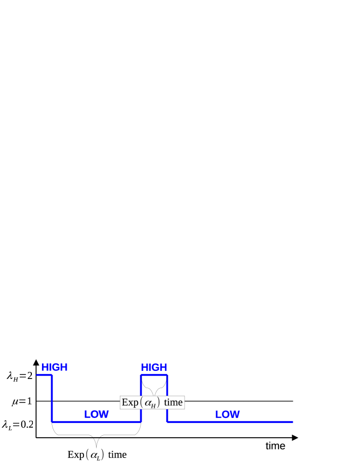
Figure 1: A time-varying arrival process with intermittent overload. The system spends $5/6$ of its time on average with a low arrival rate of $\lambda_{L}=0.2$, and $1/6$ of its time with a high arrival rate of $\lambda_{H}=2$. The average arrival rate is $\lambda=0.5$, which is below the service rate of $\mu=1$.

Intermittent overload, or fluctuating load more generally, is common in compute settings [27, 3, 12, 5, 1, 17] and also in medical setting settings [10, 2]. It is the reason that capacity provisioning is difficult, and it is the motivation behind the many papers written on dynamic capacity provisioning [6, 25, 14].

Unfortunately no closed-form formula for mean queue length is known even in the simple two-level arrivals system in Figure 1. Even tight closed-form bounds or approximations are non-existent.

History of Markovian Arrivals and Markovian Service

The intermittent overload question is a special case of the more general problem of systems with Markovian arrivals and Markovian service (MAMS). While very interesting, this question has been open for a long time. The question has been looked at via Matrix Analytic approaches and generating function approaches (see Section 2), but these methods have not led to a closed-form expression explaining how the parameters of the problem (parameters of the Markov chains) affect the performance of the system.

In recent years, there has been renewed interest in this problem. We mention a few key papers briefly here (these are described in more detail in Section 2). First, there’s a paper by Vesilo et al. [29], which derives expressions for mean queue length in a two-level arrival system, but these expressions depend on solving cubic equations, which do not provide insight into the behavior of the system. By contrast, our work provides simple closed-form bounds for the two-level arrival system, allowing insight into system behavior, while also solving the much more general MAMS system. Next, there’s a paper by Mou and Maguluri [19], which considers Markovian arrivals and Exponential service times. Aside from not handling Markovian service, the bounds proven are not closed-form. By contrast, our paper proves closed-form bounds for the MAMS setting. Finally, there’s a paper by Grosof et al. [8], which considers a narrower problem involving Poisson arrivals and a special case of Markovian service arising from the multiserver-job system. Moreover, the results in that paper are asymptotic bounds, not closed-form bounds. Our paper generalizes all of these results.

We note that while our paper focuses on the MAMS setting, an alternative way of thinking about non-i.i.d. arrivals is to define a nonstationary process where the arrival intensity depends on time $t$. While much work has been done in this direction [18, 28, 30], we note that this nonstationary setting is even less tractable than our setting, and does not allow for closed-form bounds. We focus on the MAMS setting, which allows more tractability while being broadly applicable.

Our results and approach

Summary of results: This paper proves the first closed-form bounds for mean queue length in the MAMS model. Our results are tight in heavy traffic and hold at all loads. When we specialize to the two-level system, we prove tight closed-form bounds in two additional settings: in the limit as the system switches quickly between arrival rates ($\alpha_{H},\alpha_{L}\to\infty$), and in a setting with intermittent overload setting and slow switching between arrival rates ($\lambda_{H}>\mu;\alpha_{H},\alpha_{L}\to 0$). Our main MAMS theorem is Theorem 5.1, which we use to give closed-form bounds in Corollary 5.1, and our main two-level-arrival result is Theorem 3.1, which we use to give additional closed-form bounds in Corollary 7.1.

Approach: Our general approach is a novel extension of the drift method introduced by Eryilmaz and Srikant [4]. In a nutshell, the drift method involves exploiting the fact that the stationary drift of any given random variable related to system performance is zero. The difficulty in using the drift method is choosing an appropriate test function which defines the random variable. In the past, almost all applications of the drift method have involved i.i.d. arrivals and service. The one exception is Mou and Maguluri [19], which required a complex extension to the drift method called the $m$-step drift method. Because the $m$-step drift method is much more complicated, the authors were not able to get a closed-form expression for mean queue length. Our contribution is finding a novel test function which allows for greater analytical tractability.

Our new test function introduces a new way of thinking about Markovian systems, which we call relative arrivals and relative completions. The basic idea is as follows: In an i.i.d. system, it is easy to quantify the expected number of arrivals by time $t$; call this $\mathbbm{E}[A(t)]$. For a system with Markovian arrivals, such as the two-level-arrival system, the expected number of arrivals by time $t$ depends on which arrival state the system is in at time $0$: If the system is in the high load state at time $0$, it will see more arrivals by time $t$ than if it is initially in the low load state. If we let $A_{H}(t)$ (respectively, $A_{L}(t)$) denote the number of arrivals by time $t$ for a two-level system initialized in state $H$ (respectively, $L$), then we expect $\mathbbm{E}[A_{H}(t)]>\mathbbm{E}[A_{L}(t)]$. We devise our novel test function by explicitly quantifying this difference. Specifically, we define the relative arrival quantities $\Delta(H):=\lim_{t\to\infty}\mathbbm{E}[A_{H}(t)]-\mathbbm{E}[A(t)]$ and $\Delta(L):=\lim_{t\to\infty}\mathbbm{E}[A_{L}(t)]-\mathbbm{E}[A(t)]$ (see Definition 3.1). In the general MAMS system, we also define relative completions similarly. These quantities are the heart of our novel test function.

Structure of presentation: To illustrate our method in the simplest setting possible, we start by presenting our results for the two-level arrival process, in Section 3. This allows us to use a slightly simpler test function and also greatly simplify the notation and analysis, while being an interesting result in its own right. In the next several sections (Sections 4, 5 and 6), we then solve the general MAMS system. In Section 7, we return to the two-level system to tighten our bounds in this setting.

Outline of paper

This paper is organized as follows:

• Section 2: We discuss prior work on the two-level arrivals system, and on queueing systems with Markovian arrivals and/or Markovian service.

• Section 3: We introduce the two-level arrivals system, the drift method, and the relative arrivals function specialized to this setting. We prove our main result, Theorem 3.1, for the two-level arrivals system.

• Section 4: We introduce the MAMS model, and generalize the drift method and the relative arrivals and relative completions function to the MAMS setting.

• Section 5: We state our main result, Theorem 5.1, for the general MAMS system.

• Section 6: We prove our main result for the general MAMS system.

• Section 7: We prove additional bounds for the two-level arrivals system.

• Section 8: We empirically demonstrate the accuracy and tightness of our bounds via simulation.

2 Prior work

Our goal in this paper is an explicit, simple characterization of mean queue length in the Markovian arrivals and Markovian service (MAMS) system, in terms of the parameters of the Markov chains controlling the arrival and service processes. We will discuss prior work on MAMS queues in the context of this goal, and prior work on the two-level arrival system in particular.

2.1 Generating functions and matrix analytic methods

One way of trying to analytically characterize mean queue length is by using Matrix Analytic Methods or generating function approaches.

Matrix Analytic Methods reduce the problem of deriving the stationary distribution of a MAMS system to a series of linear algebraic calculations [21, 26, 22, 16]. Similarly, generating function approaches reduce the problem to finding the roots of certain polynomials [32, 9, 20, 33, 34, 23, 29].

Unfortunately, in both methods, the solution for a general MAMS system is an extremely complex function of the system parameters: Generating function methods require extracting roots of cubic polynomials or higher degree polynomials, while Matrix Analytic methods are typically iterative numerical algorithms.

Thus, neither of these methods allows one to obtain a closed-form expression for even just the mean queue length. This obstacle exists even for simple MAMS systems such as the two-level arrivals system. In contrast, our main results, Theorems 3.1 and 5.1, give simple formulas for mean queue length, which can be used to qualitatively understand the MAMS system and the two-level arrival system in particular, and bound the behavior of both systems.

2.2 Structural and monotonicity results

Focusing on just the two-level arrival system, which we define in Section 3.1, there are a couple papers that begin to characterize the dependency of system performance on the input parameters in a qualitative way.

The first of these, by Gupta et al. [9], proves that mean queue length decreases monotonically as switching rate increases. The paper also characterizes the limiting behavior of mean queue length in the fast and slow switching limits, though in the transient overload setting it merely proves that mean queue length diverges under slow switching. Finally, the paper proves some stochastic ordering results. However, the paper does not prove closed-form expressions characterizing mean queue length outside of those limits, and does not prove bounds or convergence rate results.

The second of these, Vesilo et al. [29], extends Gupta et al. [9] by proving monotonicity results for the convexity and concavity of system performance measures such as mean queue length, by proving additional stochastic ordering results, and by covering edge cases which Gupta et al. [9] left open. However, the paper similarly does not give expressions characterizing mean queue length, nor does it prove bounds on mean queue length.

2.3 The $m$-step drift technique

A related paper to ours is Mou and Maguluri [19], which goes a step beyond prior results by analyzing a system with Markovian Arrivals and exponential service in the heavy traffic limit. While the paper proves that the scaled mean queue length $E[Q(1-\rho)]$ converges in that limit, the paper does not give a closed form expression for the limiting value, leaving it in the form of an infinite summation.

Mou and Maguluri [19]’s key analytical technique is an extension to the drift method [4] called the “$m$-step drift method,” which is considerably more complex than the original drift method. By contrast, we extend the drift method in a different, simpler direction with our relative arrival and relative completion functions, while managing to prove tighter and more explicit results.

3 Two-level arrivals

In this section, we will introduce and analyze the two-level arrival system, using a drift analysis based on our novel relative arrivals function. Our main result in this section in Theorem 3.1, which characterizes the mean queue length in the two-level arrival system. The techniques introduced in this section are then generalized to handle the entire MAMS model in Section 5.

We define the two-level arrivals model in Section 3.1. We introduce the drift method in Section 3.2. We introduce our novel relative arrivals function in Section 3.3. We sketch our proof in Section 3.4, introducing the function whose drift we will analyze. We characterize its drift in Section 3.5, and use it to prove our main result Section 3.6.

3.1 Two-level model

In the two-level arrivals model, jobs arrive to a single-server queue. Jobs wait in the queue in FCFS order. When a job reaches the head of the queue, it enters service. Job service times are exponentially distributed with rate $\mu$. All jobs are indistinguishable.

Jobs arrive according to a two-level process. The two-level arrival process is depicted in Fig. 1. The arrival process consists of two arrival rates: A high rate $\lambda_{H}$ and a low rate $\lambda_{L}$. The system switches between the two rates according to the switching rates $\alpha_{H}$, the rate of switching from $H$ to $L$, and $\alpha_{L}$, the rate of switching from $L$ to $H$. A Markovian view on this arrival process is shown in Fig. 2.

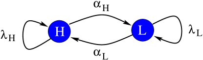
Figure 2: The arrival chain of the two-level arrival process.

Let $\lambda$ denote the long-term average arrival rate:

$$\lambda=\frac{\lambda_{H}/\alpha_{H}+\lambda_{L}/\alpha_{L}}{1/\alpha_{H}+1/\alpha_{L}}=\frac{\lambda_{H}\alpha_{L}+\lambda_{L}\alpha_{H}}{\alpha_{L}+\alpha_{H}}.$$ (1)

Let $\rho:=\lambda/\mu$ be the system load.

We will write $y$ to denote a generic arrival state, $y\in\{H,L\}$. We will write $(q,y)$ to denote a generic system state, where $q$ is the queue length and $y$ is the arrival state. Let $\bar{y}$ denote the opposite arrival state from $y$: $\bar{H}=L$ and $\bar{L}=H$. Let $Y(t)$ denote the arrival state at time $t$, and let $Y$ be the corresponding stationary random variable. We will also consider $Y^{arrival}$, the arrival-rate-weighted arrival state:

$$P(Y^{arrival}=y):=P(Y=y)\frac{\lambda_{y}}{\lambda}.$$ (2)

It is straightforward to compute the underlying distribution for $Y$. We then get $Y^{arrival}$ from (2):

$$Y =\begin{cases}H&\text{w.p. }\frac{1/\alpha_{H}}{1/\alpha_{H}+1/\alpha_{L}}=\frac{\alpha_{L}}{\alpha_{H}+\alpha_{L}}\\ L&\text{w.p. }\frac{1/\alpha_{L}}{1/\alpha_{H}+1/\alpha_{L}}=\frac{\alpha_{H}}{\alpha_{H}+\alpha_{L}}\end{cases},\qquad Y^{arrival}=\begin{cases}H&\text{w.p. }\frac{\alpha_{L}\lambda_{H}}{\alpha_{H}\lambda_{L}+\alpha_{L}\lambda_{H}}\\ L&\text{w.p. }\frac{\alpha_{H}\lambda_{L}}{\alpha_{H}\lambda_{L}+\alpha_{L}\lambda_{H}}\end{cases}.$$ (3)

3.2 Drift method

A key idea for analyzing queueing systems is that for any stationary random variable, its rate of increase must equal its rate of decrease. For instance, consider the work $W$ in an M/G/1. Using the fact that the rate of increase due to arriving jobs must equal the rate of decrease due to service, one can prove that $\rho$, the fraction of time the server is occupied, must equal $\lambda\mathbbm{E}[S]$, the product of the arrival rate and the mean job size. This balance holds for any stationary random variable. In the M/G/1, by analyzing the rate of increase and decrease of $W^{2}$, one can characterize the mean work in the system.

To formalize this concept and apply it to our system, we make use of the drift of a random variable. In a given state, the random variable’s drift is its instantaneous rate of change, in expectation over the randomness of the system. The key fact about drift is that in stationarity, the expected drift of any random variable is $0$, where the expectation is taken both over the state and the future randomness of the system.

Formally, this is captured by the instantaneous generator $G$, which is the stochastic equivalent of the derivative operator. Rather than operating on a random variable directly, it is simpler to think of $G$ as operating on a test function, a function $f$ that maps system states $(q,y)$ to real values. The instantaneous generator takes $f$ and outputs $G\circ f$, the drift of $f$.

Let $G$ specifically denote the generator operator for the two-level arrival system, which is defined as follows: For any test function $f(q,y)$,

$$G\circ f(q,y):=\lim_{t\to 0}\frac{1}{t}\mathbbm{E}[ f(Q(t),Y(t))-f(q,y)\mid Q(0)=q,Y(0)=y].$$

Now, we can state the key fact about the drift:

Lemma 3.1.

Let $f$ be a real-valued function of the MAMS system state where $\mathbbm{E}[f(Q,Y_{A},Y_{C})]<\infty.$ Then

$$\mathbbm{E}[G\circ f(Q,Y)]=0,$$ (4)

where the expectation is taken over the stationary random variables $Q,Y$.

This result is a special case of the more general result for the MAMS system, Lemma 4.1, which we prove in Appendix C. The drift method relies on finding a useful test function $f$, such that the fact that the expected drift is zero allows us to analyze the performance of the system.

3.3 Relative arrivals

Our key new tool, which will allow us to define our needed test function for the drift method, is the relative arrival function, $\Delta(i)$, which we now define.

Let $A_{y}(t)$ denote the number of arrivals by time $t$ given that the arrival process starts in state $y\in\{H,L\}$.

Definition 3.1.

The relative arrivals function $\Delta(y)$ is defined as follows:

$$\Delta(H) :=\lim_{t\to\infty}\mathbbm{E}[A_{H}(t)]-\lambda t,\qquad\Delta(L):=\lim_{t\to\infty}\mathbbm{E}[A_{L}(t)]-\lambda t.$$

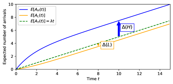
Figure 3: Expected arrivals by time $t$, starting in arrival states $H$ and $L$, and in the steady-state $Y$. Relative arrivals $\Delta(H)$ and $\Delta(L)$ are the limiting differences between these functions. Setting: $\lambda_{H}=2,\lambda_{L}=0.2,\alpha_{H}=0.5,\alpha_{L}=0.1,\mu=1,\lambda=0.5$.

As we illustrate in Fig. 3, the relative arrivals function, $\Delta(y)$, represents the difference between the expected number of arrivals given that we’re starting in state $y$ and the expected total number of arrivals. As time goes to infinity, this difference converges to a finite value.

$\Delta(H)$ and $\Delta(L)$ are related as follows:

$$\Delta(H) =\frac{\lambda_{H}-\lambda}{\alpha_{H}}+\Delta(L),\qquad\Delta(L)=\frac{\lambda_{L}-\lambda}{\alpha_{L}}+\Delta(H).$$ (5)

To see why (5) holds, note that $\lambda_{H}-\lambda$ is the difference in arrival rates between $H$ and the long-term rate, and $\frac{1}{\alpha_{H}}$ is the time for which that difference accrues. After this time, the system transitions to state $L$.

To characterize the exact values of $\Delta(H)$ and $\Delta(L)$, we can use the fact that the time-average value of $\Delta$ is zero: $\mathbbm{E}[\Delta(Y)]=0$, which we prove for the more general MAMS system in Lemma 4.3. As a result:

$$\Delta(H) =\alpha_{H}\frac{\lambda_{H}-\lambda_{L}}{(\alpha_{H}+\alpha_{L})^{2}},\qquad\Delta(L)=\alpha_{L}\frac{\lambda_{L}-\lambda_{H}}{(\alpha_{H}+\alpha_{L})^{2}}.$$ (6)

The drift of the relative arrivals function is nicely behaved: $G\circ\Delta(y)=\lambda-\lambda_{y}$. This follows from Definition 3.1: The $\mathbbm{E}[A_{y}(t)]$ term contributes $\lambda_{y}$ to the drift, while the $\lambda t$ term contributes $\lambda$. This property is generalized to the MAMS system and proven in Corollary B.1.

3.4 Developing our test function

We come up with a new test function $f_{\Delta}(q,y)$ for the drift method that combines both the queue length and the relative arrivals introduced in the last subsection.

Definition 3.2.

$f_{\Delta}(q,y):=(q+\Delta(y))^{2}-\Delta(y)^{2}=q(q+2\Delta(y)).$

The intuition for the use of the test function $f_{\Delta}(q,y)$ is that on its own, the queue length $q$ changes at a state-dependent rate, which is hard to analyze. Specifically, jobs arrive at the rate $\lambda_{y}$ and complete at the rate $\mu$, so the queue length $q$ has drift $\lambda_{y}-\mu$, assuming $q>0$.

We want to “smooth out” the instantaneous rate of change of $q$. Specifically, we want a function which:

• has a constant drift, in all system states where $q>0$, and

• differs from $q$ by a bounded amount.

Recall from Section 3.3 that the drift of $\Delta(y)$ is $\lambda-\lambda_{y}$. Thus, the function $q+\Delta(y)$ has a constant drift of $\lambda-\mu$ in all system states where $q>0$.

Thus, $q+\Delta(y)$ is a smoothed-out proxy for the queue length $q$ with constant drift, making it tractable for analysis. We set $f_{\Delta}(q,y)$ to be a smoothed-out proxy for the square of the queue length, as applying the generator $G$ gives information about the expected derivative of the test function, and hence information about $\mathbbm{E}[Q]$. Specifically, as we show in Lemma 3.3, the drift of $f_{\Delta}(q,y)$ separates cleanly: It has a $(\lambda-\mu)q$ term, and terms that do not depend on $q$. Then, in Theorem 3.1, we apply the fact that the drift is zero in stationarity (Lemma 3.1), allowing us to characterize $\mathbbm{E}[Q]$.

3.5 Lemmas for the two-level system

First, let’s calculate the drift of a generic test function in the two-level system.

Lemma 3.2.

For any test function $f$ in the two-level system, its instantaneous drift in a particular system state $(q,y)$ can be expressed as

$$G\circ f(q,y)=\lambda_{y}(f(q+1,y)-f(q,y))+\alpha_{y}(f(q,\bar{y})-f(q,y))+\mu(f(q-1+u,y)-f(q,y)),$$

where $u:=(1-q)^{+}=\mathbbm{1}\{q=0\}$ denotes unused service, and $\bar{y}$ is the opposite arrival state from $y$.

Proof.

In a given state of the two-level system $(q,y)$, there are three events that can occur: arrival, change of the arrival state $y$, and completion, if $q>0$. These three events each contribute a corresponding term to the drift of the generic test function $f$. ∎

Now, we can calculate the drift for the special test function $f_{\Delta}(q,y)=q(q+2\Delta(y))$.

Lemma 3.3.

For any system state $(q,y)$ of the two-level system, the instantaneous drift is

$$G\circ f_{\Delta}(q,y)=2(\lambda-\mu)q+2(\lambda_{y}-\mu(1-u))\Delta(y)+\lambda_{y}+\mu(1-u).$$ (7)

Proof.

By Lemma 3.2 and the definition of $f_{\Delta}(q,y)$,

$$G\circ f_{\Delta}(q,y)=\, \lambda_{y}\big{(}(q+1)(q+1+2\Delta(y))-q(q+2\Delta(y))\big{)}$$ (8)

$$+\alpha_{y}\big{(}q(q+2\Delta(\bar{y}))-q(q+2\Delta(y))\big{)}$$ (9)

$$+\mu\big{(}(q-1+u)(q-1+u+2\Delta(y))-q(q+2\Delta(y))\big{)}.$$ (10)

Let us simplify each term in the expression. Each term will simplify to an affine function of $q$: A linear term in $q$, plus an additive offset. The slope of some of these affine functions will depend on $y$, but we will show that for the overall drift, the slope does not depend on $y$, due to our choice of test function.

For the arrivals term, (8),

$$\lambda_{y}\big{(}(q+1)(q+1+2\Delta(y))-q(q+2\Delta(y))\big{)}=\,2\lambda_{y}q+\lambda_{y}\big{(}2\Delta(y)+1\big{)}.$$

For the switching term, (9),

$$\alpha_{y}\big{(}q(q+2\Delta(\bar{y}))-q(q+2\Delta(y))\big{)}=2\alpha_{y}q(\Delta_{A}(\bar{y})-\Delta(y)).$$

For the completions term, (10),

$$\mu\big{(}(q-1+u)(q-1+u+2\Delta(y))-q(q+2\Delta(y))\big{)}=-2\mu q+\mu(1-u)\big{(}-2\Delta(y)+1\big{)},$$

where we make use of the facts that $qu=0$ and that $(1-u)^{2}=(1-u)$, noting that $(1-u)\in\{0,1\}$.

Combining the above calculations, we find that

$$G\circ f_{\Delta}(q,y) =2(\lambda_{y}+\alpha_{y}(\Delta(\bar{y})-\Delta(y))-\mu)q$$ (11)

$$+2(\lambda_{y}-\mu(1-u))\Delta(y)+\lambda_{y}+\mu(1-u).$$

Now, we want to simplify the $\lambda_{y}+\alpha_{y}(\Delta(\bar{y})-\Delta(y))$ coefficient in (11). To do so, let us use a relationship demonstrated in Section 3.3, namely (5):

$$\Delta(y) =\frac{\lambda_{y}-\lambda}{\alpha_{y}}+\Delta(\bar{y})\implies\lambda=\lambda_{y}+\alpha_{y}(\Delta(\bar{y})-\Delta(y)).$$

Thus, the linear term in (11) simplifies to a term which does not depend on $y$, as desired:

$$G\circ f_{\Delta}(q,y)=2(\lambda-\mu)q+2(\lambda_{y}-\mu(1-u))\Delta(y)+\lambda_{y}+\mu(1-u).\qed$$

3.6 Main result for two-level system

Theorem 3.1.

In the two-level arrivals system with exponential service rate, the mean queue length is:

$$\mathbbm{E}[Q] =\frac{\rho(\mathbbm{E}[\Delta(Y^{arrival})]+1)}{1-\rho}+\mathbbm{E}[\Delta(Y)\mid Q=0],\text{ where}$$ (12)

$$\mathbbm{E}[\Delta(Y^{arrival})] =\frac{(\lambda_{H}-\lambda_{L})^{2}\alpha_{L}\alpha_{H}}{\lambda(\alpha_{H}+\alpha_{L})^{3}},$$

$$\mathbbm{E}[\Delta(Y)\mid Q=0] =\frac{\lambda_{H}-\lambda_{L}}{\alpha_{H}+\alpha_{L}}\left(P(Y=H\mid Q=0)-\frac{\alpha_{L}}{\alpha_{H}+\alpha_{L}}\right).$$

Proof.

We start with the result of Lemma 3.3:

$$G\circ f_{\Delta}(q,y)=2(\lambda-\mu)q+2(\lambda_{y}-\mu(1-u))\Delta(y)+\lambda_{y}+\mu(1-u).$$ (13)

Recall Lemma 3.1, the key drift-method lemma, which states that for (essentially) any test function, $f(q,y)$, we have $\mathbbm{E}[G\circ f(Q,Y)]=0$, where $(Q,Y)$ is the stationary random variable for the system state. In particular, $\mathbbm{E}[G\circ f_{\Delta}(Q,Y)]=0$. We will use this fact to characterize $\mathbbm{E}[Q]$. More specifically, because $f_{\Delta}(q,y)$ grows polynomially in $q$, we show it satisfies Lemma 3.1 in Lemma C.2.

Taking the expectation of (13), we find that

$$0 =\mathbbm{E}[G\circ f_{\Delta}(Q,Y)]$$

$$=2(\lambda-\mu)\mathbbm{E}[Q]+2\mathbbm{E}_{y\sim Y}[\lambda_{y}\Delta(y)]-2\mu\mathbbm{E}[\Delta(y)]+2\mu\mathbbm{E}[\Delta(Y)\mathbbm{1}\{Q=0\}]+\lambda+\mu P(Q>0)$$

$$=2(\lambda-\mu)\mathbbm{E}[Q]+2\mathbbm{E}_{y\sim Y}[\lambda_{y}\Delta(y)]+2\mu\mathbbm{E}[\Delta(Y)\mathbbm{1}\{Q=0\}]+\lambda+\mu P(Q>0).$$ (14)

In taking this expectation, we use the facts that $\lambda:=\mathbbm{E}[\lambda_{Y}]$, that $\mathbbm{E}[\Delta(Y)]=0$, and that $u:=\mathbbm{1}\{q=0\}$. Note that the $(\lambda-\mu)q$ term in (13) allows us to get a $\mathbbm{E}[Q]$ term in (14).

To simplify (14), note that because the system has an exponential service rate, $P(Q>0)=\rho=\frac{\lambda}{\mu}$, by Lemma A.1. Thus:

$$0=\, (\lambda-\mu)\mathbbm{E}[Q]+\mathbbm{E}_{y\sim Y}[\lambda_{y}\Delta(y)]+(\mu-\lambda)\mathbbm{E}[\Delta(Y)\mid Q=0]+\lambda.$$ (15)

Recall that we defined $Y^{arrival}$ to be the arrival-weighted state of the arrival process. In particular, from (2), $P(Y^{arrival}=y):=P(Y=y)\frac{\lambda_{y}}{\lambda}$. As a result, $\mathbbm{E}_{y\sim Y}[\lambda_{y}\Delta(y)]=\lambda\mathbbm{E}[\Delta(Y^{arrival})]$, and (15) becomes:

$$0 =(\lambda-\mu)\mathbbm{E}[Q]+\lambda\mathbbm{E}[\Delta(Y^{arrival})]+(\mu-\lambda)\mathbbm{E}[\Delta(Y)\mid Q=0]+\lambda$$

$$\mathbbm{E}[Q] =\frac{\rho(\mathbbm{E}[\Delta(Y^{arrival})]+1)}{1-\rho}+\mathbbm{E}[\Delta(Y)\mid Q=0].$$

Using the values of $\Delta$ from (6) and the distribution for $Y^{arrival}$ from (3), we can compute $\mathbbm{E}[\Delta(Y^{arrival})]$ and compute $\mathbbm{E}[\Delta(Y)\mid Q=0]$ up to the value of $P(Y=H\mid Q=0)$, which we bound in Section 7. ∎

Note that plugging in the bound $P(Y=H\mid Q=0)>0$ immediately gives a strong lower bound on $\mathbbm{E}[Q]$. In Section 7, we prove tight upper bounds on $P(Y=H\mid Q=0)$ in both the quick switching limit ($\alpha_{H},\alpha_{L}\to\infty$) and in the slow switching limit ($\alpha_{H},\alpha_{L}\to 0$), giving tight results in both regimes.

Even without any bounds on $P(Y=H\mid Q=0)$, Theorem 3.1 already tightly characterizes mean response time in the $\rho\to 1$ limit (the heavy traffic limit), holding $\alpha_{H}$ and $\alpha_{L}$ constant:

Corollary 3.1.

In the two-level arrivals system, the scaled mean queue length in the heavy traffic limit converges to $\lim_{\rho\to 1}(1-\rho)\mathbbm{E}[Q]=\mathbbm{E}[\Delta(Y^{arrival})]+1.$

This holds because $\mathbbm{E}[\Delta(Y)\mid Q=0]$ is bounded by $\Delta(L)$ and $\Delta(H)$, which are bounded in the $\rho\to 1$ limit.

In the more general setting of Markovian arrivals and Markovian service (MAMS), we prove Theorem 5.1, a generalization of our two-level result Theorem 3.1, which can handle any number of arrival rates, as well as Markov modulated service rates. This results in a similar heavy traffic result, Corollary 5.2.

4 MAMS model and definitions

We now turn to the general setting of Markovian arrivals and Markovian service (MAMS), where the arrival process and the completions process are both Markov chains.

Like the two-level arrival system introduced in Section 3.1, the MAMS system consists of a single-server queue. Jobs wait in the queue in FCFS order. When a job reaches the head of the queue, it enters service. After some time in service, the job completes. All jobs are indistinguishable. Jobs arrive according to an arrival process which we define in Section 4.1, and complete according to a completion process which we define in Section 4.2. After introducing the MAMS model, Sections 4.3, 4.4 and 4.5 generalize our discussion of the drift process, the notion of relative arrivals (and completions), and the test function from what we saw in Section 3. The main results for the MAMS model are stated in Section 5.

Our goal is to bound the mean queue length in the MAMS system, with bounds that are tight in heavy traffic. We seek to generalize Theorem 3.1, our main result for the two-level arrivals system.

4.1 Arrivals

We start by generalizing the arrival process to be a general finite-state continuous-time Markov chain. In Section 3.1, the arrival process had only two states, high arrival intensity and low arrival intensity. There were two types of updates in that arrival process: Jobs arriving, which happened with rate $\lambda_{H}$ and $\lambda_{L}$, and state changes, which happened with rate $\alpha_{H}$ and $\alpha_{L}$.

In the more general MAMS setting, we must track both the initial and final state of a state change, and we also allow for a job to arrive simultaneously with the state change.

We thus use the following more general notation: Let the state space of the arrival chain be some finite set $\mathbbm{A}$. For a given pair of states $i\neq j\in\mathbbm{A}$, the system may transition from $i$ to $j$ with an arrival, or from $i$ to $j$ without an arrival. We will denote the rate of the former transition as $r_{i,j,1}$, and of the later transition as $r_{i,j,0}$. In general, we will write the transition rate as $r_{i,j,a}$, where the $a$ parameter indicates whether an arrival occurs during a transition. As a special case, self-transitions may only occur with an arrival: $r_{i,i,1}$ may be nonzero, $r_{i,i,0}$ is always zero.

For example, in the two-level system of Section 3, $\mathbbm{A}=\{H,L\}$, and the nonzero transition rates are:

$$r_{H,H,1}=\lambda_{H},\quad r_{L,L,1}=\lambda_{L},\quad r_{H,L,0}=\alpha_{H},\quad r_{L,H,0}=\alpha_{L}.$$

We assume that the arrival chain is irreducible. Let $\lambda$ be the long-term arrival rate, as in Section 3.1. Let $Y_{A}(t)$ be a random variable denoting the state of the arrival chain at time $t$. Let $Y_{A}$ be the corresponding stationary random variable. Let $Y_{A}^{arrival}$ be the arrival-rate-weighted arrival state, defined as follows:

$$P(Y_{A}^{arrival}=j):=\frac{\sum_{i\in\mathbbm{A}}P(Y_{A}=i)r_{i,j,1}}{\lambda}.$$

Note that $Y_{A}(t),Y_{A},$ and $Y_{A}^{arrival}$ correspond to $Y(t),Y,$ and $Y^{arrival}$ from Section 3.1. The subscript _A is added to differentiate the arrival chain from the completion chain, which will use the subscript _C.

We will use $\cdot$ in the rate subscripts when aggregating multiple related rates. For instance, $r_{i,\cdot,\cdot}:=\sum_{j,a}r_{i,j,a}$. As a special case, we will define $\lambda_{i}=r_{i,\cdot,1}$ to be the total instantaneous arrival rate in state $i$.

4.2 Completions

In the two-level arrivals model in Section 3, completions always occurred at rate $Exp(\mu)$. In the general MAMS model, we allow the completion chain to be a general finite-state continuous-time Markov chain.

Paralleling the arrival chain defined in Section 4.1, we let the state space of the completion chain be some finite set $\mathbbm{C}$. For each $i,j\in\mathbbm{C}$, the system may transition from $i$ to $j$ with a completion or without a completion, at rates $s_{i,j,0}$ and $s_{i,j,1}$ respectively. As before, $s_{i,i,1}$ may be nonzero, but $s_{i,i,0}=0$. We write these rates as $s_{i,j,c}$, where the $c$ parameter denotes whether a completion occurs during a transition. Again, we assume the completion chain is irreducible.

One important note: A completion transition may occur when there are no jobs present in the system. If this happens, the completion process’s state change still occurs, and the queue remains empty. We will refer to such a completion as an “unused completion.”

Let $\mu$ denote the long-term rate of completions, whether used or unused.

As an example, in the two-level system there was only a single completion state, which we may arbitrarily call $X$. Then $\mathbbm{C}=\{X\}$. The sole completion transition rate was $s_{X,X,1}=\mu$.

We define $Y_{C}(t),Y_{C}$, and $Y_{C}^{comp}$ to correspond to $Y_{A}(t),Y_{A},$ and $Y_{A}^{arrival}$ from Section 4.1. In particular,

$$P(Y_{C}^{comp}=j):=\frac{\sum_{i\in\mathbbm{C}}P(Y_{C}=i)s_{i,j,1}}{\mu}.$$

We define the load $\rho$ to be the ratio $\lambda/\mu$. Our bounds hold for all loads $\rho$, and are tight in the heavy-traffic limit, as $\rho\to 1$.

In our main result for the two-level arrival system, Theorem 3.1, we make use of an expectation of the form $\mathbbm{E}[\cdot\mid Q=0]$, conditioning on the system state when the queue is empty. In the MAMS setting, we condition the system state when when unused completions occur. We will write this expectation as $\mathbbm{E}_{U}[\cdot]$. Note that in the two-level system, because of the exponential service process and the PASTA property [31], these two expectations coincide: $\mathbbm{E}_{U}[\cdot]=\mathbbm{E}[\cdot\mid Q=0]$. We define the expectation $\mathbbm{E}_{U}[\cdot]$ in more detail in Appendix A.

As with the arrival process, we use $\cdot$ to aggregate related rates, and define $\mu_{i}=s_{i,\cdot,1}$ to correspond to $\lambda_{i}$.

4.3 Drift method

In the general MAMS model, we continue using the drift method which we discussed in Section 3.2, using the fact that the rate of change of any random variable is zero in steady state. Formally, the rate of change of a random variable is captured by the drift of a test function. Here a test function $f$ is any real-valued function of the state of the MAMS system, $(q,i_{A},i_{C})$, where $q$ denotes the total number of jobs, and $i_{A}$ and $i_{C}$ denote the states of the arrival and service processes, respectively. The drift of the test function $G\circ f(q,i_{A},i_{C})$ is defined as

$$G\circ f(q,i_{A},i_{C}):=\lim_{t\to 0}\frac{1}{t}\mathbbm{E}[ f(Q(t),Y_{A}(t),Y_{C}(t))-f(q,i_{A},i_{C})\mid Q(0)=q,Y_{A}(0)=i_{A},Y_{C}(0)=i_{C}].$$

The operator $G$ is called the instantaneous generator, which takes a test function $f$ as input and gives the drift of the test function $G\circ f$ as output. The instantaneous generator can be seen as the stochastic equivalent of the derivative operator.

The lemma below shows that the expected value of the $G\circ f$ in steady state is zero, generalizing Lemma 3.1 to the MAMS system. We prove Lemma 4.1 in Appendix C.

Lemma 4.1.

Let $f$ be a test function for which $\mathbbm{E}[f(Q,Y_{A},Y_{C})]<\infty.$ Then

$$\mathbbm{E}[G\circ f(Q,Y_{A},Y_{C})]=0.$$ (16)

All test functions $f$ that we will use with (16) will grow at a polynomial rate in $q$, which we show satisfy Lemma 4.1 in Lemma C.2.

Similar to Lemma 3.2, Lemma 4.2 below provides the expression for the drift of a generic function in the MAMS system. Lemma 4.2 is standard in the drift method literature, and we have specialized it to this system. We prove Lemma 4.2 in Appendix C.

Lemma 4.2.

For any real-valued function $f$ of the state of the MAMS system,

$$G\circ f(q,i_{A},i_{C}) =\sum_{j_{A}\in\mathbbm{A},a\in\{0,1\}}r_{i_{A},j_{A},a}\left(f(q+a,j_{A},i_{C})-f(q,i_{A},i_{C})\right)$$

$$+\sum_{j_{C}\in\mathbbm{C},c\in\{0,1\}}s_{i_{C},j_{C},c}\left(f(q-c+u,i_{A},j_{C})-f(q,i_{A},i_{C})\right),$$

where $u=(c-q)^{+}$ denotes the unused service.

4.4 Relative arrivals and completions

In Section 3.3, we introduced the concept of the relative arrivals function. In the MAMS setting, we denote this relative arrivals function as $\Delta_{A}(i)$, and we also introduce the relative completions function $\Delta_{C}(i)$, defined equivalently.

Let $A_{i}(t)$ denote the number of arrivals by time $t$ given that the arrival chain starts in state $i\in\mathbbm{A}$ at time $t=0$. Let $C_{i}(t)$ denote the number of completions by time $t$ given that the completion chain starts in state $i\in\mathbbm{C}$ at time $t=0$.

Definition 4.1.

Define the relative arrivals and relative completions functions $\Delta_{A}(i),\Delta_{C}(i)$ as follows:

$$\Delta_{A}(i) :=\lim_{t\to\infty}\mathbbm{E}[A_{i}(t)]-\lambda t,\qquad\Delta_{C}(i):=\lim_{t\to\infty}\mathbbm{E}[C_{i}(t)]-\mu t.$$

We verify that these limits always converge to a finite value in Appendix B. These functions can be seen as the relative value function of the Markov reward process where a reward of 1 is received whenever an arrival or completion occurs, respectively. We can therefore calculate their values explicitly by solving the corresponding Poisson equation, given in Lemma B.1, along with Lemma 4.3, which states that these quantities have zero expected value in stationarity:

Lemma 4.3.

$\mathbbm{E}[\Delta_{A}(Y_{A})]=0$, $\mathbbm{E}[\Delta_{C}(Y_{C})]=0$.

Proof.

Note that $[Y_{A}(t)\mid Y_{A}(0)=Y_{A}]\sim Y_{A}$. As a result, $\mathbbm{E}[A_{Y_{A}}(t)]=\lambda t$ for any $t$. Then by definition, $\mathbbm{E}[\Delta_{A}(Y_{A})]=\lim_{t\to\infty}(\mathbbm{E}[A_{Y_{A}}(t)]-\lambda t)=0$. Similarly, $\mathbbm{E}[\Delta_{C}(Y_{C})]=0$. ∎

Another important property of $\Delta_{A}(i)$ and $\Delta_{C}(i)$ are their drifts:

Corollary B.1 1.

$G\circ\Delta_{A}(i_{A})=\lambda-\lambda_{i_{A}},G\circ\Delta_{C}(i_{C})=\mu-\mu_{i_{C}}.$

Corollary B.1 follows from the Poisson equation, Lemma B.1, and it is proven in Appendix B.

4.5 Test function

In order to characterize $\mathbbm{E}[Q]$, we introduce the test function $f_{\Delta_{A},\Delta_{C}}(q,i_{A},i_{C})$, which generalizes the two-level arrival test function defined in Definition 3.2 to the MAMS system.

Definition 4.2.

$f_{\Delta_{A},\Delta_{C}}(q,i_{A},i_{C}):=q(q+2\Delta_{A}(i_{A})-2\Delta_{C}(i_{C})).$

The intuition for this test function again comes from finding a smooth proxy for the queue length $q$. In the two-level system, we used $q+\Delta(y)$ as a proxy for $q$, to capture the influence of the state-dependent arrival rate in the two-level system, In the MAMS system, both the arrival rates and completion rates are state-dependent, so we use $q+\Delta_{A}(i_{A})-\Delta_{C}(i_{C})$ as a smooth proxy for $q$.

To characterize mean queue length, we need a proxy for the square of the queue length. In the two-level system, we used $q(q+2\Delta(y))$ as our proxy for the square of queue length. In the MAMS system, $f_{\Delta_{A},\Delta_{C}}(q,i_{A},i_{C})$ fulfils the same role.

5 Results

We now present the main of the paper: a closed-form formula for the mean queue length in the MAMS system. This will be proven in Section 6.

Theorem 5.1 (Mean queue length).

In the MAMS system, the mean queue length is given by:

$$\mathbbm{E}[Q]=\frac{\rho\mathbbm{E}[\Delta_{A}(Y_{A}^{arrival})]+\mathbbm{E}[\Delta_{C}(Y_{C}^{comp})]+\rho}{1-\rho}+\mathbbm{E}_{U}[\Delta_{A}(Y_{A})-\Delta_{C}(Y_{C}^{comp})],$$

where $\mathbbm{E}_{U}[\cdot]$ was defined in Section 4.2:

$$\mathbbm{E}_{U}[\Delta_{A}(Y_{A})-\Delta_{C}(Y_{C}^{comp}))] =\frac{\mathbbm{E}[(\mu_{Y_{C}}\Delta_{A}(Y_{A})-\sum_{j_{C}\in\mathbbm{C}}s_{Y_{C},j_{C},1}\Delta_{C}(j_{C})))\mathbbm{1}\{Q=0\}]}{\mu-\lambda}.$$

Our formula consists of a fully-explicit primary term and a secondary term (the $\mathbbm{E}_{U}[\cdot]$ term) which depends on the behavior of the MAMS system when the queue is empty, captured by the expectation over the unused service $\mathbbm{E}_{U}[\cdot]$. Theorem 5.1 generalizes our two-level result, Theorem 3.1. The $\mathbbm{E}[\Delta(Y)\mid Q=0]$ term in Theorem 3.1 becomes the $\mathbbm{E}_{U}[\cdot]$ term in Theorem 5.1, and terms are introduced for the Markovian service process. One can exactly compute the $\Delta_{A}(\cdot)$ and $\Delta_{C}(\cdot)$ functions by solving the corresponding Poisson equations, as discussed in Section 4.4.

As one consequence of Theorem 5.1, note that $\mathbbm{E}_{U}[\Delta_{A}(Y_{A})-\Delta_{C}(Y_{C}^{comp})]$ is bounded by the maximum and minimum possible values of $\Delta_{A}$ and $\Delta_{C}$, yielding the following simple bounds:

Corollary 5.1.

Let $\Delta_{A}^{\max}$ and $\Delta_{A}^{\min}$ be the maximum and minimum values of $\Delta_{A}(i_{A})$ over all arrival states $i_{A}$, and define $\Delta_{C}^{\max}$ and $\Delta_{C}^{\min}$ similarly. In the MAMS system, the mean queue length is bounded by

$$\Delta_{A}^{\min}-\Delta_{C}^{\max}\leq\mathbbm{E}[Q]-\frac{\rho\Delta_{A}(Y_{A}^{arrival})+\Delta_{C}(Y_{C}^{comp})+\rho}{1-\rho} \leq\Delta_{A}^{\max}-\Delta_{C}^{\min}.$$

Proof.

This corollary follows immediately from Theorem 5.1, once we recall that the arrival and completion state spaces $\mathbbm{A}$ and $\mathbbm{C}$ are finite, and that the relative arrivals and completions functions always converge, as discussed in Section 4.4. ∎

Note that these bounds converge in the $\rho\to 1$ limit, as $\Delta_{A}^{\max},\Delta_{A}^{\min},\Delta_{C}^{\max},$ and $\Delta_{C}^{\min}$ remain bounded in that limit, allowing us to exactly characterize the heavy traffic behavior of the system:

Corollary 5.2.

In the MAMS system, the scaled mean queue length in the heavy traffic limit converges:

$$\lim_{\rho\to 1}(1-\rho)\mathbbm{E}[Q]=\mathbbm{E}[\Delta_{A}(Y_{A}^{arrival})]+\mathbbm{E}[\Delta_{C}(Y_{C}^{comp})]+1.$$

6 Proofs for MAMS system

We will follow a similar structure to that used in Section 3:

• Lemma 6.1 sets up the formula for the drift of our chosen test function $f_{\Delta_{A},\Delta_{C}}$, which we introduced in Section 4.5, splitting the drift into an arrivals term and a completions term.

• Lemmas 6.2 and 6.4 simplify the arrivals and completions drift terms.

• Lemmas 6.3 and 6.5 compute the steady-state expectations of the arrivals and completions drift terms.

• In Section 6.2, we prove Theorem 5.1 using our expected drift results and the fact that expected drift in steady state is zero to characterize mean queue length $\mathbbm{E}[Q]$.

Lemmas 6.2 and 6.4 collectively generalize Lemma 3.3 from the two-level system to the MAMS system, while Lemmas 6.3, 6.5 and 5.1 collectively generalize Theorem 3.1.

6.1 Key lemmas

We start by deriving an initial formula for the drift of our test function $f_{\Delta_{A},\Delta_{C}}$, which we introduced in Section 4.5. We separate this formula into two terms: An arrivals term $g_{A}$ and a completions term $g_{C}$.

Lemma 6.1 (Formula for drift of $f_{\Delta_{A},\Delta_{C}}$).

For any MAMS system and any system state $(q,i_{A},i_{C})$,

$$G\circ f_{\Delta_{A},\Delta_{C}}(q,i_{A},i_{C})=g_{A}(q,i_{A},i_{C})+g_{C}(q,i_{A},i_{C}),$$

$$\text{where }g_{A}(q,i_{A},i_{C}):=$$ (17)

$$\sum_{j_{A}\in\mathbbm{A},a}r_{i_{A},j_{A},a}\left((q+a)(q+a+2\Delta_{A}(j_{A})-2\Delta_{C}(i_{C}))-q(q+2\Delta_{A}(i_{A})-2\Delta_{C}(i_{C}))\right),$$

$$\text{and where }g_{C}(q,i_{A},i_{C}):=$$ (18)

$$\sum_{j_{C}\in\mathbbm{C},c}s_{i_{C},j_{C},c}\left((q-c+u)(q-c+u+2\Delta_{A}(i_{A})-2\Delta_{C}(j_{C}))-q(q+2\Delta_{A}(i_{A})-2\Delta_{C}(i_{C}))\right).$$

Proof.

Follows immediately from Lemma 4.2. ∎

Now, we simplify the $g_{A}$ term.

Lemma 6.2.

For any MAMS system and any system state $(q,i_{A},i_{C})$,

$$g_{A}(q,i_{A},i_{C})=2\lambda q+(1-2\Delta_{C}(i_{C}))\lambda_{i_{A}}+2\sum_{j_{A}\in\mathbbm{A}}r_{i_{A},j_{A},1}\Delta_{A}(j_{A}).$$ (19)

Proof.

We start by simplifying $g_{A}(q,i_{A},i_{C})$. Recall the definition of $g_{A}$, (17):

$$g_{A}(q,i_{A},i_{C})=\sum_{j_{A},a}r_{i_{A},j_{A},a}\left((q+a)(q+a+2\Delta_{A}(j_{A})-2\Delta_{C}(i_{C}))-q(q+2\Delta_{A}(i_{A})-2\Delta_{C}(i_{C}))\right).$$ (20)

Let us simplify the bracketed term inside the summation:

$$(q+a)(q+a+2\Delta_{A}(j_{A})-2\Delta_{C}(i_{C}))-q(q+2\Delta_{A}(i_{A})-2\Delta_{C}(i_{C}))$$

$$=2q(a+\Delta_{A}(j_{A})-\Delta_{A}(i_{A}))+a(a-2\Delta_{C}(i_{C})+2\Delta_{A}(j_{A})).$$ (21)

Let us substitute (21) back into (20):

$$g_{A}(q,i_{A},i_{C})=\, 2q\sum_{j_{A},a}r_{i_{A},j_{A},a}(a+\Delta_{A}(j_{A})-\Delta_{A}(i_{A}))$$ (22)

$$+\sum_{j_{A},a}r_{i_{A},j_{A},a}a(a-2\Delta_{C}(i_{C})+2\Delta_{A}(j_{A})).$$ (23)

We will separately simplify (22) and (23).

For (22), we prove in Corollary B.1 that for any initial state $i_{A}$,

$$\sum_{j_{A},a}r_{i_{A},j_{A},a}(a+\Delta_{A}(j_{A})-\Delta_{A}(i_{A}))=\lambda.$$

This follows from the definition of the relative arrivals function $\Delta_{A}$.

For (23), note that $a\in\{0,1\}$:

$$\sum_{j_{A},a}r_{i_{A},j_{A},a}a(a-2\Delta_{C}(i_{C})+2\Delta_{A}(j_{A}))=(1-2\Delta_{C}(i_{C}))\lambda_{i_{A}}+2\sum_{j_{A}}r_{i_{A},j_{A},1}\Delta_{A}(j_{A}).$$

Combining our simplifications, we find that

$$g_{A}(q,i_{A},i_{C}) =2\lambda q+(1-2\Delta_{C}(i_{C}))\lambda_{i_{A}}+2\sum_{j_{A}}r_{i_{A},j_{A},1}\Delta_{A}(j_{A}).\qed$$

Now, we characterize the expectation of $g_{A}$ over the steady state of the MAMS system.

Lemma 6.3 (Mean of arrivals term $g_{A}$).

For any MAMS system,

$$\mathbbm{E}[g_{A}(Q,Y_{A},Y_{C})]=\lambda(2\mathbbm{E}[Q]+2\mathbbm{E}[\Delta_{A}(Y_{A}^{arrival})]+1).$$ (24)

Proof.

Let us begin with the simplified expression for $g_{A}$ from Lemma 6.2:

$$g_{A}(q,i_{A},i_{C}) =2\lambda q+(1-2\Delta_{C}(i_{C}))\lambda_{i_{A}}+2\sum_{j_{A}}r_{i_{A},j_{A},1}\Delta_{A}(j_{A}).$$

$$\mathbbm{E}[g_{A}(Q,Y_{A},Y_{C})] =2\lambda\mathbbm{E}[Q]+\mathbbm{E}[(1-2\Delta_{C}(Y_{C}))\lambda_{Y_{A}}]$$ (25)

$$\quad+2\sum_{i_{A},j_{A}}P(Y_{A}=i_{A})r_{i_{A},j_{A},1}\Delta_{A}(j_{A}).$$ (26)

We simplify (25) and (26) separately. For (25), note that $Y_{A}$ and $Y_{C}$ are independent, as the arrival process and completions process update independently. Note also that $\mathbbm{E}[\Delta_{C}(Y_{C}))]=0$, as shown in Lemma 4.3, and that $\mathbbm{E}[\lambda_{Y_{A}}]=\lambda$, which is the definition of $\lambda$. Thus, we can simplify the second term of (25):

$$\mathbbm{E}[(1-2\Delta_{C}(Y_{C}))\lambda_{Y_{A}}]=\mathbbm{E}[(1-2\Delta_{C}(Y_{C}))]\mathbbm{E}[\lambda_{Y_{A}}] =\lambda.$$ (27)

As for (26), recall from Section 4.1 the definition of $Y_{A}^{arrival}$, the arrival-rate-weighted arrival state:

$$P(Y_{A}^{arrival}=j):=\frac{\sum_{i\in\mathbbm{A}}P(Y_{A}=i)r_{i,j,1}}{\lambda}.$$

As a result, we can simplify (26):

$$\sum_{i_{A},j_{A}}P(Y_{A}=i_{A})r_{i_{A},j_{A},1}\Delta_{A}(j_{A}) =\lambda\sum_{j_{A}}P(Y_{A}^{arrival}=j_{A})\Delta_{A}(j_{A})=\lambda\mathbbm{E}[\Delta_{A}(Y_{A}^{arrival})].$$ (28)

Substituting (27) and (28) into (25), we find that

$$\mathbbm{E}[g_{A}(Q,Y_{A},Y_{C})] =\lambda(2\mathbbm{E}[Q]+2\mathbbm{E}[\Delta_{A}(Y_{A}^{arrival})]+1).\qed$$

Now, we switch to the completions term, $g_{C}$. We start by simplifying $g_{C}$. Lemma 6.4 mirrors Lemma 6.2, but with some additional complications due to unused service when $q=0$.

Lemma 6.4 (Simplification of the completion term $g_{C}$).

For any MAMS system and any system state $(q,i_{A},i_{C})$,

$$g_{C}(q,i_{A},i_{C})=-2\mu q+\Big{(}(1-2\Delta_{A}(i_{A}))\mu_{i_{C}}+2\sum_{j_{C}\in\mathbbm{C}}s_{i_{C},j_{C},1}\Delta_{C}(j_{C})\Big{)}\mathbbm{1}\{q>0\}.$$ (29)

Proof.

Recall the definition of $g_{C}(q,i_{A},i_{C})$ from Lemma 4.2:

$$g_{C}(q,i_{A},i_{C}):=\sum_{j_{C},c}s_{i_{C},j_{C},c}\left((q-c+u)(q-c+u+2\Delta_{A}(i_{A})-2\Delta_{C}(j_{C}))-q(q+2\Delta_{A}(i_{A})-2\Delta_{C}(i_{C}))\right),$$

where $u:=(c-q)^{+}$ is the amount of unused service caused by a specific transition. Note that $u\in\{0,1\}$.

Let us simplify the bracketed term inside the summation:

$$(q-c+u)(q-c+u+2\Delta_{A}(i_{A})-2\Delta_{C}(j_{C}))-q(q+2\Delta_{A}(i_{A})-2\Delta_{C}(i_{C}))$$

$$=2q(-c+u-\Delta_{C}(j_{C})+\Delta_{C}(i_{C}))+(-c+u)(-c+u+2\Delta_{A}(i_{A})-2\Delta_{C}(j_{C}))$$

$$=-2q(c+\Delta_{C}(j_{C})-\Delta_{C}(i_{C}))+c(c-2\Delta_{A}(i_{A})+2\Delta_{C}(j_{C}))+u(2q-2c+u+2\Delta_{A}(i_{A})-2\Delta_{C}(j_{C})).$$ (30)

We substitute (30) back to the definition of $g_{C}(q,i_{A},i_{C})$ and get

$$g_{C}(q,i_{A},i_{C}) =-2q\sum_{j_{C},c}s_{i_{C},j_{C},c}(c+\Delta_{C}(j_{C})-\Delta_{C}(i_{C}))$$ (31)

$$+\sum_{j_{C},c}s_{i_{C},j_{C},c}c(c-2\Delta_{A}(i_{A})+2\Delta_{C}(j_{C}))$$ (32)

$$+\sum_{j_{C},c}s_{i_{C},j_{C},c}u(2q-2c+u+2\Delta_{A}(i_{A})-2\Delta_{C}(j_{C})).$$ (33)

For the term in (31), we prove in Corollary B.1 that

$$\sum_{j_{C},c}s_{i_{C},j_{C},c}(c+\Delta_{C}(j_{C})-\Delta_{C}(i_{C}))=\mu.$$

so the term in (31) can be simplified as

$$-2q\sum_{j_{C},c}s_{i_{C},j_{C},c}(c+\Delta_{C}(j_{C})-\Delta_{C}(i_{C}))=-2\mu q.$$

For the term in (32), note that $c\in\{0,1\}$, so

$$\sum_{j_{C},c}s_{i_{C},j_{C},c}c(c-2\Delta_{A}(i_{A})+2\Delta_{C}(j_{C})) =\sum_{j_{C}}s_{i_{C},j_{C},1}(1-2\Delta_{A}(i_{A})+2\Delta_{C}(j_{C}))$$

$$=(1-2\Delta_{A}(i_{A}))\mu_{i_{C}}+2\sum_{j_{C}}s_{i_{C},j_{C},1}\Delta_{C}(j_{C}).$$

For the term in (33), recall that $u=(c-q)^{+}$, so $u\in\{0,1\}$, and $u=1$ if and only if $c=1$ and $q=0$. We thus simplify the term in (33) as

$$\sum_{j_{C},c}s_{i_{C},j_{C},c}u(2q-2c+u+2\Delta_{A}(i_{A})-2\Delta_{C}(j_{C}))$$

$$=\sum_{j_{C}}s_{i_{C},j_{C},1}(-1+2\Delta_{A}(i_{A})-2\Delta_{C}(j_{C}))\mathbbm{1}\{q=0\}$$

$$=-\Big{(}(1-2\Delta_{A}(i_{A}))\mu_{i_{C}}+2\sum_{j_{C}}s_{i_{C},j_{C},1}\Delta_{C}(j_{C})\Big{)}\mathbbm{1}\{q=0\}.$$

Combining our simplifications, we find that

$$g_{C}(q,i_{A},i_{C})=-2\mu q+\Big{(}(1-2\Delta_{A}(i_{A}))\mu_{i_{C}}+2\sum_{j_{C}}s_{i_{C},j_{C},1}\Delta_{C}(j_{C})\Big{)}\mathbbm{1}\{q>0\}.\qed$$

Lemma 6.5 (Mean of completions term $g_{C}$).

For any MAMS system,

$$\mathbbm{E}[g_{C}(Q,Y_{A},Y_{C})]=-2\mu\mathbbm{E}[Q]+\lambda+2\mu\mathbbm{E}[\Delta_{C}(Y_{C}^{comp})]+2\mathbbm{E}[h_{C0}(Y_{A},Y_{C})\mathbbm{1}\{Q=0\}],$$

where $h_{C0}$ is defined as follows:

$$h_{C0}(i_{A},i_{C}) =\mu_{i_{C}}\Delta_{A}(i_{A})-\sum_{j_{C}\in\mathbbm{C}}s_{i_{C},j_{C},1}\Delta_{C}(j_{C}),$$

$$\mathbbm{E}[h_{C0}(Y_{A},Y_{C})\mathbbm{1}\{Q=0\}] =(\mu-\lambda)\mathbbm{E}_{U}[\Delta_{A}(Y_{A})-\Delta_{C}(Y_{C}^{comp})].$$

Proof.

By the simplified formula of $g_{C}(q,i_{A},i_{C})$ in Lemma 6.4, we have

$$\mathbbm{E}[g_{C}(Q,Y_{A},Y_{C})]=-2\mu\mathbbm{E}[Q]+\mathbbm{E}[\big{(}(1-2\Delta_{A}(Y_{A}))\mu_{Y_{C}}+2\sum_{j_{C}}s_{Y_{C},j_{C},1}\Delta_{C}(j_{C})\big{)}\mathbbm{1}\{Q>0\}].$$ (34)

We can decompose the second term of (34) using the fact that $\mathbbm{1}\{Q>0\}=1-\mathbbm{1}\{Q=0\}$. Observe that

$$\mathbbm{E}[(1-2\Delta_{A}(Y_{A}))\mu_{Y_{C}}+2\sum_{j_{C}}s_{Y_{C},j_{C},1}\Delta_{C}(j_{C})] =\mathbbm{E}[1-2\Delta_{A}(Y_{A})]\mathbbm{E}[\mu_{Y_{C}}]+2\mu\mathbbm{E}[\Delta_{C}(Y_{C}^{comp})]$$

$$=\mu+2\mu\mathbbm{E}[\Delta_{C}(Y_{C}^{comp})],$$

where the first equality uses the independence of $Y_{A}$ and $Y_{C}$, and the definition of $Y_{C}^{comp}$; and the second equality is due to $\mathbbm{E}[\mu_{Y_{C}}]=\mu$ and $\mathbbm{E}[\Delta_{A}(Y_{A})]=0$. Next, we deal with the term

$$\mathbbm{E}[\big{(}(1-2\Delta_{A}(Y_{A}))\mu_{Y_{C}}+2\sum_{j_{C}}s_{Y_{C},j_{C},1}\Delta_{C}(j_{C})\big{)}\mathbbm{1}\{Q=0\}]$$

$$=\mathbbm{E}[\mu_{Y_{C}}\mathbbm{1}\{Q=0\}]+\mathbbm{E}[\big{(}-2\Delta_{A}(Y_{A})\mu_{Y_{C}}+2\sum_{j_{C}}s_{Y_{C},j_{C},1}\Delta_{C}(j_{C})\big{)}\mathbbm{1}\{Q=0\}]$$

$$=\mu-\lambda-2\mathbbm{E}[h_{C0}(Y_{A},Y_{C})\mathbbm{1}\{Q=0\}],$$

where the last equality is due to $\mathbbm{E}[\mu_{Y_{C}}\mathbbm{1}\{Q=0\}]=\mu-\lambda$, which we prove in Lemma A.1. Plugging the above calculations into (34), we get

$$\mathbbm{E}[g_{C}(Q,Y_{A},Y_{C})] =-2\mu\mathbbm{E}[Q]+\mu+2\mu\mathbbm{E}[\Delta_{C}(Y_{C}^{comp})]-\mu+\lambda+2\mathbbm{E}[h_{C0}(Y_{A},Y_{C})\mathbbm{1}\{Q=0\}]$$

$$=-2\mu\mathbbm{E}[Q]+\lambda+2\mu\mathbbm{E}[\Delta_{C}(Y_{C}^{comp})]+2\mathbbm{E}[h_{C0}(Y_{A},Y_{C})\mathbbm{1}\{Q=0\}].$$

Equivalently, we can write the last term $\mathbbm{E}\left[h_{C0}(Y_{A},Y_{C})\mathbbm{1}\{Q=0\}\right]$ in terms of $\mathbbm{E}_{U}[\cdot]$:

$$\mathbbm{E}\left[h_{C0}(Y_{A},Y_{C})\mathbbm{1}\{Q=0\}\right] =\mathbbm{E}[\mu_{Y_{C}}\Delta_{A}(Y_{A})\mathbbm{1}\{Q=0\}]-\mathbbm{E}[\sum_{j_{C}}s_{Y_{C},j_{C},1}\Delta_{C}(j_{C}))\mathbbm{1}\{Q=0\}]$$

$$=(\mu-\lambda)\mathbbm{E}_{U}[\Delta_{A}(Y_{A})]-(\mu-\lambda)\mathbbm{E}_{U}[\Delta_{C}(Y_{C}^{comp})]$$

$$=(\mu-\lambda)\mathbbm{E}_{U}[\Delta_{A}(Y_{A})-\Delta_{C}(Y_{C}^{comp})].\qed$$

6.2 Proof of main result: Theorem 5.1

Theorem 5.1 2.

In the MAMS system, the mean queue length is given by:

$$\mathbbm{E}[Q]=\frac{\rho\mathbbm{E}[\Delta_{A}(Y_{A}^{arrival})]+\mathbbm{E}[\Delta_{C}(Y_{C}^{comp})]+\rho}{1-\rho}+\mathbbm{E}_{U}[\Delta_{A}(Y_{A})-\Delta_{C}(Y_{C}^{comp})],$$

where recall the definition of $\mathbbm{E}_{U}[\cdot]$ in Section 4.2 that

$$\mathbbm{E}_{U}[\Delta_{A}(Y_{A})-\Delta_{C}(Y_{C}^{comp}))] =\frac{\mathbbm{E}[(\mu_{Y_{C}}\Delta_{A}(Y_{A})-\sum_{j_{C}\in\mathbbm{C}}s_{Y_{C},j_{C},1}\Delta_{C}(j_{C})))\mathbbm{1}\{Q=0\}]}{\mu-\lambda}.$$

Proof.

Recall Lemma 6.1, $G\circ f_{\Delta_{A},\Delta_{C}}(q,i_{A},i_{C})=g_{A}(q,i_{A},i_{C})+g_{C}(q,i_{A},i_{C})$. Because $\mathbbm{E}[G\circ f_{\Delta_{A},\Delta_{C}}(Q,Y_{A},Y_{C})]=0$ by Lemma 4.1, we have

$$\mathbbm{E}[g_{A}(Q,Y_{A}Y_{C})]+\mathbbm{E}[g_{C}(Q,Y_{A},Y_{C})]=0.$$

Using Lemmas 6.3 and 6.5, we get

$$\lambda(2\mathbbm{E}[Q]+2\mathbbm{E}[\Delta_{A}(Y_{A}^{arrival})]+1)$$

$$-2\mu\mathbbm{E}[Q]+\lambda+2\mu\mathbbm{E}[\Delta_{C}(Y_{C}^{comp})]+2(\mu-\lambda)\mathbbm{E}_{U}[\Delta_{A}(Y_{A})-\Delta_{C}(Y_{C}^{comp})]=0.$$

Rearranging the terms,

$$2(\mu-\lambda)\mathbbm{E}[Q] =2\lambda\mathbbm{E}[\Delta_{A}(Y_{A}^{arrival})]+2\mu\mathbbm{E}[\Delta_{C}(Y_{C}^{comp})]+2\lambda+2(\mu-\lambda)\mathbbm{E}_{U}[\Delta_{A}(Y_{A})-\Delta_{C}(Y_{C}^{comp})]$$

$$\mathbbm{E}[Q] =\frac{\lambda\mathbbm{E}[\Delta_{A}(Y_{A}^{arrival})]+\mu\mathbbm{E}[\Delta_{C}(Y_{C}^{comp})]+\lambda}{\mu-\lambda}+\mathbbm{E}_{U}[\Delta_{A}(Y_{A})-\Delta_{C}(Y_{C}^{comp})]$$

$$=\frac{\rho\Delta_{A}(Y_{A}^{arrival})+\Delta_{C}(Y_{C}^{comp})+\rho}{1-\rho}+\mathbbm{E}_{U}[\Delta_{A}(Y_{A})-\Delta_{C}(Y_{C}^{comp})].\qed$$

7 Bounds on two-level system when $Q=0$

We proved Theorem 5.1, a general result characterizing mean queue length in the MAMS system. As a corollary, in Corollary 5.1, we proved explicit bounds on mean queue length in the MAMS system. However, in the two-level arrivals system, we can prove tighter bounds on mean queue length, because we know more about the dynamics of the system. In this section, we prove such tighter bounds.

In the two-level system, we proved Theorem 3.1, which characterized mean queue length $\mathbbm{E}[Q]$, with the only remaining uncertainty being the probability $P(Y=H\mid Q=0)$ that the system is in the $H$ arrival state while the queue is empty. In this section, we prove Theorem 7.1, upper bounding $P(Y=H\mid Q=0)$. These bounds complement the straightforward lower bound $P(Y=H\mid Q=0)\geq 0$.

Theorem 7.1.

In the two-level arrival system, $P(Y=H\mid Q=0)$ is bounded as follows:

$$P(Y=H\mid Q=0) \leq P(Y=H)=\frac{\alpha_{L}}{\alpha_{L}+\alpha_{H}}.$$ (35)

Additionally, if the system is intermittently overloaded ($\lambda_{H}>\mu$), the following bound holds:

$$P(Y=H\mid Q=0) \leq\frac{1}{1-\rho}\frac{1}{\lambda_{H}-\mu}\frac{\alpha_{H}\alpha_{L}}{\alpha_{H}+\alpha_{L}}.$$ (36)

We will prove Theorem 7.1 in Section 7.1.

These bounds are tight in different asymptotic regimes: (35) is tight in the $\alpha_{H},\alpha_{L}\to\infty$ limit, where the arrival state switches rapidly, while (36) is tight in the $\alpha_{H},\alpha_{L}\to 0$ limit, as the arrival state switches slowly. These bounds complement our heavy-traffic result for the two-level system, Corollary 3.1.

Using these bounds alongside Theorem 3.1, we can derive tight bounds on mean queue length in the two-level arrival system:

Corollary 7.1.

In the two-level arrivals system with exponential service rate, the mean queue length is bounded as follows:

$$\mathbbm{E}[Q] \geq\frac{\rho}{1-\rho}\left(\frac{(\lambda_{H}-\lambda_{L})^{2}\alpha_{L}\alpha_{H}}{\lambda(\alpha_{H}+\alpha_{L})^{3}}+1\right)-\frac{\lambda_{H}-\lambda_{L}}{\alpha_{H}+\alpha_{L}}\frac{\alpha_{L}}{\alpha_{H}+\alpha_{L}},$$ (37)

$$\mathbbm{E}[Q] \leq\frac{\rho}{1-\rho}\left(\frac{(\lambda_{H}-\lambda_{L})^{2}\alpha_{L}\alpha_{H}}{\lambda(\alpha_{H}+\alpha_{L})^{3}}+1\right).$$ (38)

If the system is intermittently overloaded ($\lambda_{H}>\mu$), then additionally

$$\mathbbm{E}[Q] \leq\frac{\rho}{1-\rho}\left(\frac{(\lambda_{H}-\lambda_{L})^{2}\alpha_{L}\alpha_{H}}{\lambda(\alpha_{H}+\alpha_{L})^{3}}+1\right)-\frac{\lambda_{H}-\lambda_{L}}{\alpha_{H}+\alpha_{L}}\frac{\alpha_{L}}{\alpha_{H}+\alpha_{L}}\left(1-\frac{\alpha_{H}}{(1-\rho)(\lambda_{H}-\mu)}\right).$$ (39)

Proof.

These bounds follow from combining Theorem 3.1 with bounds on $P(Y=H\mid Q=0)$. (37) follows from the fact that $P(Y=H\mid Q=0)\geq 0$. (38) follows from (35). (39) follows from (36). ∎

In the non-intermittently-overloaded case ($\lambda_{H}<\mu$), prior work has proven basic bounds on $\mathbbm{E}[Q]$. Gupta et al. [9] proved that $\mathbbm{E}[Q]$ is bounded below by the mean queue length of a M/M/1 with arrival rate $\lambda$ and completion rate $\mu$, and bounded above by a weighted mixture of two M/M/1s: one with arrival rate $\lambda_{H}$ and one with arrival rate $\lambda_{L}$. While these bounds are not tight, it is challenging to use our techniques to prove tighter results in this setting, which we leave to future work.

7.1 Proof of Theorem 7.1

Proof.

We start by considering the general two-level arrival system, with no restriction on $\lambda_{H}$ and $\mu$. We will prove (35):

$$P(Y=H\mid Q=0) \leq P(Y=H)=\frac{\alpha_{L}}{\alpha_{L}+\alpha_{H}}.$$

To prove this result, we make use of prior work by Gupta et al. [9] to bound the probability $P(Q=0\mid Y=L)$, the probability that the queue is empty given that the arrival rate is low.

Let $\pi_{0}^{L}$ be the probability that the queue is empty at the moment when the system switches from $L$ to $H$. By [9, Theorem 3], $P(Q=0\mid Y=L)=\pi_{0}^{L}$. During the proof of [9, Theorems 6 and 7], it is proven that there exists some $\chi\in(0,1)$ such that $\pi_{0}^{L}/\pi_{0}^{H}=(\mu-\chi\lambda_{L})/(\mu-\chi\lambda_{H}).$

Because $\lambda_{L}\leq\lambda_{H}$, we know that $\pi_{0}^{L}\geq\pi_{0}^{H}$, and hence that $P(Q=0\mid Y=L)\geq P(Q=0\mid Y=H)$.

To quantify $P(Q=0)$, note that in all systems, the fraction of potential service events which go unused is $1-\rho$. In the two-level arrival system, because the completion process is exponential, it is therefore the case that $P(Q=0)=1-\rho$.

Thus, we know that $P(Q=0\mid Y=L)\geq 1-\rho$, and that $P(Q=0\mid Y=H)\leq 1-\rho$. We can therefore bound $P(Y=H\mid Q=0)$:

$$P(Y=L\mid Q=0) \geq P(Y=L)=\frac{\alpha_{H}}{\alpha_{H}+\alpha_{L}},\quad P(Y=H\mid Q=0)\leq P(Y=H)=\frac{\alpha_{L}}{\alpha_{H}+\alpha_{L}}.$$

Now, consider the intermittently overloaded two-level arrival system, where $\lambda_{H}>\mu$. We will prove (36):

$$P(Y=H\mid Q=0) \leq\frac{1}{1-\rho}\frac{1}{\lambda_{H}-\mu}\frac{\alpha_{H}\alpha_{L}}{\alpha_{H}+\alpha_{L}}.$$

The intuition behind this bound is that if $\lambda_{H}>\mu$, the queue length grows throughout each $Y=H$ interval, and hence the queue is rarely empty ($Q$ is rarely $0$) during such an interval.

To make this idea rigorous, consider an overloaded M/M/1 with arrival rate $\lambda_{H}$ greater than the service rate $\mu$, in which the queue is empty at time 0 ($Q(0)=0$). The expected total amount of time for which $Q(t)=0$ in the overloaded M/M/1 system is finite: by a standard calculation, one can show that this expected duration is $1/(\lambda_{H}-\mu)$. That amount of time is an upper bound on the expected amount of time for which $Q=0$ during each $Y=H$ interval in the two-level system.

Thus, the expected time that two-level system spends in the state $y=H,q=0$ during each $y=H$ interval is at most $1/(\lambda_{H}-\mu)$, regardless of the initial queue length at the beginning of the interval. A larger initial queue length and a finite interval length can only decrease the expected time for which the system is empty.

To bound $P(Y=H\land Q=0)$, we use a renewal-reward argument, with two kinds of cycles: A switching cycle, consisting of a $y=H$ interval followed by a $y=L$ interval, and a zero-switching cycle, which is a renewal cycle with a renewal point whenever the system changes from $y=L$ to $y=H$ at a moment when $Q=0$. Let $Z$ be a random variable denoting the number of switching cycles within each zero-switching cycle. Note that $Z$ has a finite mean because the two-level system is positive recurrent with $\lambda<\mu$.

We now apply the renewal-reward theorem [13], with the renewal period being the zero-switching cycles, and the reward being the time spent in the state $Y=H,Q=0$:

$$P(Y=H\land Q=0) =\frac{\mathbbm{E}[\text{$Y=H\land Q=0$ duration during a zero-switching cycle}]}{\mathbbm{E}[\text{Length of a zero-switching cycle}]}.$$

The lengths of the switching cycles within the zero-switching cycles are i.i.d. with expected length $\frac{1}{\alpha_{H}}+\frac{1}{\alpha_{L}}$, and the length of zero-switching cycle is a stopping time with mean $E[Z](\frac{1}{\alpha_{H}}+\frac{1}{\alpha_{L}})$. The amount of time for which $Y=H\land Q=0$ during the switching cycles are correlated, but only via the length of the queue at the start of the cycle. Regardless of that queue length, the expected time for which $Y=H\land Q=0$ per switching cycle is at most $1/(\lambda_{H}-\mu)$. As a result,

$$P(Y=H\land Q=0) \leq\frac{\mathbbm{E}[Z]/(\lambda_{H}-\mu)}{\mathbbm{E}[Z](1/\alpha_{H}+1/\alpha_{L})}=\frac{1/(\lambda_{H}-\mu)}{1/\alpha_{H}+1/\alpha_{L}}.$$

Recall that $P(Q=0)=1-\rho$, because the system has exponential service. As a result,

$$P(Y=H\mid Q=0)\leq\frac{1}{1-\rho}\frac{1/(\lambda_{H}-\mu)}{1/\alpha_{H}+1/\alpha_{L}}=\frac{1}{1-\rho}\frac{1}{\lambda_{H}-\mu}\frac{\alpha_{H}\alpha_{L}}{\alpha_{H}+\alpha_{L}}.\quad\qed$$

Note that (36) scales linearly with $\alpha_{H},\alpha_{L}$, so it converges to 0 in the $\alpha_{H},\alpha_{L}\to 0$ limit.

8 Simulation

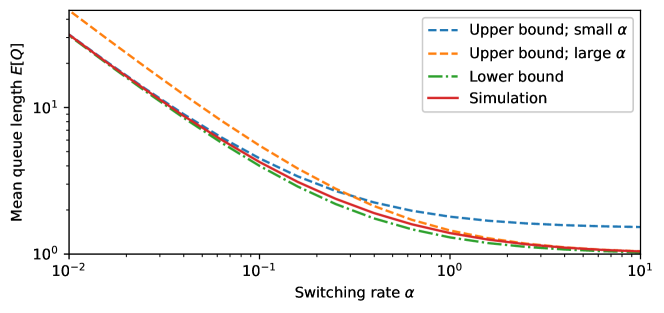
Figure 4: Simulation and bounds for mean queue length $\mathbbm{E}[Q]$ in two-level system with intermittent overload, under varying switching rates $\alpha_{H},\alpha_{L}$. Setting: $\lambda_{H}=2,\lambda_{L}=0.2,\alpha_{H}=5\alpha_{L},\mu=1,\rho=0.5$. Overall switching rate $\alpha:=(\alpha_{H}+\alpha_{L})/2$. Bounds given in Corollary 7.1: The upper bound which is tight for small $\alpha$ is (39), for large $\alpha$ is (38), and the lower bound is (37). Simulated $10^{8}$ arrivals.

We have characterized the mean queue length for the MAMS system, with bounds given in Corollary 5.1. We have proven even tighter bounds for the two-level arrival system in Corollary 7.1.

In this section, we simulate mean queue length for the two-level arrival system and a more general MAMS system, and compare our simulations to our bounds, to validate our bounds and demonstrate their tightness.

In Fig. 4, we simulate an intermittently overloaded two-level arrivals system under a variety of switching rates $\alpha_{H},\alpha_{L}$. In Fig. 4, we have moderate overall load, because $\rho=0.5$, but significant periods of intermittent overload, because $\lambda_{H}=2>\mu=1$.

Fig. 4 shows that our bounds in Corollary 7.1 are tight in both the fast-switching limit (large $\alpha$, short periods of time in each arrival state) and the slow-switching limit (small $\alpha$, long periods of time in each arrival state), with our bounds tightly and accurately constraining the mean queue length in both limits. Specifically, (37) and (38) are tight in the fast-switching limit, while (37) and (39) are tight in the slow-switching limit. Moreover, our bounds are reasonably tight at all switching rates $\alpha$, even outside the asymptotic regime, with a maximum absolute error of $0.5$ jobs, and a maximum relative error of 23%.

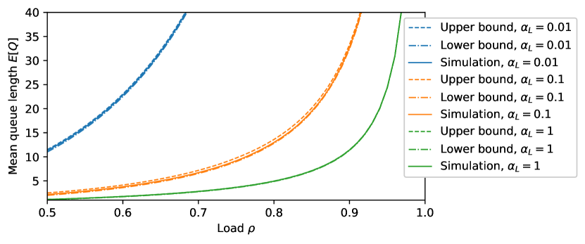
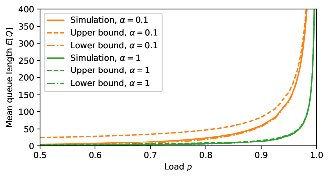
Figure 5: Simulation and bounds for mean queue length $\mathbbm{E}[Q]$ in two-level system with intermittent overload, under varying load $\rho$, for three different values of $\alpha_{L}$. Setting: $\lambda_{H}=4\rho,\lambda_{L}=0.4\rho,\alpha_{H}=5\alpha_{L},\mu=1$. Bounds given in Corollary 7.1: Upper bound is minimum of (38) and (39). Simulated $10^{8}$ arrivals.

Figure 6: Setting: MAMS queue with three arrivals levels: $[0.3\rho,2\rho,2.2\rho]$, and three completions levels: [0.5, 1.0, 3.0]. The system remains in each arrival state and each service state for time $Exp(\alpha)$, then moves cyclically to the next rate in the list, wrapping around. Bounds given in Corollary 5.1. Simulated $10^{9}$ arrivals.

In Fig. 6, we simulate a two-level system under a variety of loads $\rho$, and under three different pairs of switching rates $\alpha_{H},\alpha_{L}$. We compare the simulated mean response time against our bounds from Corollary 7.1. In every configuration of load $\rho$ and switching rates $\alpha_{H},\alpha_{L}$ simulated in Fig. 6, the absolute gap between our upper and lower bounds is at most 1 job. The relative error between our bounds drops towards zero as the system moves towards heavy traffic ($\rho\to 1$), in each setting.

In Fig. 6, we simulate a MAMS system with three levels of arrival rates and three levels of completion rates, under varying loads $\rho$. The system cycles between three possible arrival rates and three possible completion rates. Recall that as with all MAMS systems, the arrival chain and completions chain evolve independently. The switching rate from each arrival and completion state to the next is a fixed rate $\alpha$. In Fig. 6, we show two switching rates $\alpha$. We compare the simulated mean queue lengths $\mathbbm{E}[Q]$ against our bounds from Corollary 5.1. Fig. 6 illustrates that our bounds are tight in heavy traffic, even for the more complex MAMS system, confirming the heavy-traffic limit result in Corollary 5.2. Unlike the two-level arrival setting illustrated in Figs. 4 and 6, our bounds are not as tight in the general MAMS setting in light traffic (i.e., for small $\rho$), especially for slower switching settings (low $\alpha$). Proving more precise bounds on $\mathbbm{E}[Q]$ for general MAMS systems in light traffic is left for future work.

9 Conclusion

We analyze the Markovian arrivals Markovian service (MAMS) system, using a novel extension to the drift method based on the concepts of relative arrivals and relative completions. These concepts provide a new way of looking at the MAMS system, which allows us to concisely capture the impact of the correlated arrivals and completions on mean queue length. We derive the first fully explicit bounds on mean queue length in the MAMS system, with bounds that are tight in heavy traffic.

Moreover, in the important special case of the two-level arrivals system under intermittent overload, we prove significantly stronger bounds which are tight both in the fast-switching and slow-switching limits.

An important direction for future work is to improve the tightness of our bounds both for the two-level system without intermittent overload, and in the general MAMS system outside of heavy traffic.

Another important direction for future work is to analyze MAMS systems with infinite arrival and/or completions chains. Our proof of the main theorem, Theorem 5.1, holds in such systems, assuming appropriate conditions on the arrivals and completions chains, but it does not immediately imply a tight bound on mean queue length.

Appendix A Expectation over unused service

We now formally define the expectation $\mathbbm{E}_{U}[\cdot]$, the expectation at moments of unused service. Unused service occurs at rate $\mu_{i_{C}}$ whenever $q=0$.

For any test function $f(q,i_{A},i_{C})$, we define its expectation at moments of unused service $\mathbbm{E}_{U}[\cdot]$ as

$$\mathbbm{E}_{U}[f(Q,Y_{A},Y_{C})] :=\frac{\mathbbm{E}[\mu_{Y_{C}}f(Q,Y_{A},Y_{C})\mathbbm{1}\{Q=0\}]}{\mathbbm{E}[\mu_{Y_{C}}\mathbbm{1}\{Q=0\}]}=\frac{\mathbbm{E}[\mu_{Y_{C}}f(Q,Y_{A},Y_{C})\mathbbm{1}\{Q=0\}]}{\mu-\lambda},$$

where the second equality holds because $\mathbbm{E}[\mu_{Y_{C}}\mathbbm{1}\{Q=0\}]=\mu-\lambda$ by Lemma A.1.

In the special case of exponential service times, $\mu_{i_{C}}=\mu$ for any $i_{C}\in\mathbbm{C}$, so

$$\mathbbm{E}_{U}[f(Q,Y_{A},Y_{C})] =\mathbbm{E}[f(Q,Y_{A},Y_{C})\mid Q=0]=\frac{\mathbbm{E}[f(Q,Y_{A},Y_{C})\mathbbm{1}\{Q=0\}]}{1-\rho}.$$

We will also write $\mathbbm{E}_{U}[f(Y_{C}^{comp})]$, which is defined as the expectation of $f(i_{C})$ with respect to the distribution of $Y_{C}$ right after unused service, i.e., the completions that happen during $Q=0$. Formally,

$$\mathbbm{E}_{U}[f(Y_{C}^{comp})] :=\mathbbm{E}_{U}\Bigg{[}\sum_{j_{C}\in\mathbbm{C}}\frac{s_{Y_{C},j_{C},1}}{\mu_{Y_{C}}}f(j_{C})\Bigg{]}=\frac{\mathbbm{E}\left[\sum_{j_{C}\in\mathbbm{C}}s_{Y_{C},j_{C},1}f(j_{C})\mathbbm{1}\{Q=0\}\right]}{\mathbbm{E}\left[\mu_{Y_{C}}\mathbbm{1}\{Q=0\}\right]}.$$

Note the similarity with the definition of $Y_{C}^{comp}$ in Section 4.2.

We now characterize the rate of unused service in the system, namely completion transitions that occur when the queue is empty:

Lemma A.1.

The rate of unused service is $\mu-\lambda$: $\mathbbm{E}_{i\sim Y_{C}}[\mu_{i}\mathbbm{1}\{Q=0\}]=\mu-\lambda$.

Proof.

The long-run arrival rate is $\lambda$. The long-run rate of completion transitions is $\mu$. Nonetheless, the long-run arrival and completion rate must be equal, because the system is stable. Thus the long-run completion rate is $\lambda$. The only way that a completion transition can not cause a completion is if the queue is empty, causing unused service. As a result, the rate of unused service must be $\mu-\lambda$. ∎

Note that by Lemma A.1, in systems with exponential service such as the two-level arrivals system, $P(Q>0)=\lambda/\mu=\rho$.

Appendix B Relative arrivals and completions

First, we verify that $\Delta_{A}$ and $\Delta_{C}$, the relative arrivals and relative completions functions, are well-defined and finite. Note that $\Delta_{A}$ is the relative value function of a average-reward Markov Reward process with Markov chain matching the arrival process and reward equal to the arrival rate $\lambda_{i}$. By Puterman [24, Section 8.2.1], this relative value is well-defined and finite for any finite-state Markov chain. $\Delta_{C}$ is equivalent.

Next, we establish two systems of equations, equivalent to the Poisson equation for MDPs, which can be used to calculate $\Delta_{A}(i)$ in each state $i\in\mathbbm{A}$ (or $\Delta_{C}(i)$ in each state $i\in\mathbbm{C}$), up to an additive constant. Incorporating Lemma 4.3, which states that $\mathbbm{E}[\Delta_{A}(Y_{A})]=0$ (or $\mathbbm{E}[\Delta_{C}(Y_{A})]=0$), uniquely characterizes $\Delta_{A}(i)$ (or $\Delta_{C}(i)$).

Lemma B.1.

For any arrivals chain, the relative arrivals function $\Delta_{A}$ and relative completions function $\Delta_{C}$ satisfy the following systems of equations:

$$\forall i\in\mathbbm{A},\quad\Delta_{A}(i) =\frac{\lambda_{i}-\lambda}{r_{i,\cdot,\cdot}}+\sum_{j\in\mathbbm{A}}\frac{r_{i,j,\cdot}}{r_{i,\cdot,\cdot}}\Delta_{A}(j),\quad\forall i\in\mathbbm{C},\quad\Delta_{C}(i)=\frac{\mu_{i}-\mu}{s_{i,\cdot,\cdot}}+\sum_{j\in\mathbbm{C}}\frac{s_{i,j,\cdot}}{s_{i,\cdot,\cdot}}\Delta_{C}(j).$$ (40)

Proof.

Let us start with Definition 4.1: $\Delta_{A}(i):=\lim_{t\to\infty}\mathbbm{E}[A_{i}(t)]-\lambda t$, where $A_{i}(t)$ denotes the number of arrivals by time $t$, given that the arrivals chain starts from state $i$.

Let us split up $\mathbbm{E}[A_{i}(t)]-\lambda t$, the expression inside the limit, into two time periods: Until the arrival chain next undergoes a transition, and after that time. The transition occurs after $Exp(r_{i,\cdot,\cdot})$ time, or $\frac{1}{r_{i,\cdot,\cdot}}$ expected time. Prior to the transition, $\mathbbm{E}[A_{i}(t)]-\lambda t$ accrues at rate $\lambda_{i}-\lambda$. We use $Y_{A}^{next}$ to denote the state after the transition. Then we have the expression:

$$\Delta_{A}(i) =\frac{\lambda_{i}-\lambda}{r_{i,\cdot,\cdot}}+\lim_{t\to\infty}\mathbbm{E}[A_{Y_{A}^{next}}(t)]-\lambda t=\frac{\lambda_{i}-\lambda}{r_{i,\cdot,\cdot}}+\mathbbm{E}[\Delta_{A}(Y_{A}^{next})].$$

Finally, note that $P(Y_{A}^{next}=j)=\frac{r_{i,j,\cdot}}{r_{i,\cdot,\cdot}}$, allowing us to derive the equations for $\Delta_{A}(i)$ in (40). The equations for $\Delta_{C}(i)$ can be proved similarly. ∎

As a corollary of Lemma B.1, we characterize the change in the value of $\Delta_{A}(i)$ when a transition occurs in the arrival chain, and the change in the value of $\Delta_{C}(i)$ when a transition occurs in the completion chain.

Corollary B.1.

In the MAMS system, the effect of arrival (or completion) on relative arrival (or relative completion) satisfies:

$$\forall i\in\mathbbm{A},\quad \sum_{j\in\mathbbm{A},a\in\{0,1\}}r_{i,j,a}(\Delta_{A}(j)-\Delta_{A}(i)+a)=\lambda,$$ (41)

$$\forall i\in\mathbbm{C},\quad \sum_{j\in\mathbbm{C},c\in\{0,1\}}s_{i,j,c}(\Delta_{C}(j)-\Delta_{C}(i)+c)=\mu.$$ (42)

Equivalently, for any $i\in\mathbbm{A}$, $G\circ\Delta_{A}(i)=\lambda-\lambda_{i}$; for any $i\in\mathbbm{C}$, $G\circ\Delta_{C}(i)=\mu-\mu_{i}$.

Proof.

By (40) in Lemma B.1, for any $i\in\mathbbm{A}$, $\Delta_{A}(i)=\frac{\lambda_{i}-\lambda}{r_{i,\cdot,\cdot}}+\sum_{j\in\mathbbm{A}}\frac{r_{i,j,\cdot}}{r_{i,\cdot,\cdot}}\Delta_{A}(j)$. Multiplying both sides by $r_{i,\cdot,\cdot}$, rearranging the terms, and expanding $r_{i,\cdot,\cdot},r_{i,j,\cdot},$ and $\lambda_{i}$, we get (41). (42) follows similarly.

It can be convenient to express (41) and (42)in terms of $G\circ\Delta_{A}$ and $G\circ\Delta_{C}$. Note that by Lemma 4.2, $G\circ\Delta_{A}(i)=\sum_{j\in\mathbbm{A}}r_{i,j,\cdot}(\Delta_{A}(j)-\Delta_{A}(i)).$ Thus, $G\circ\Delta_{A}(i)=\lambda-\lambda_{i}$ and $G\circ\Delta_{C}(i)=\mu-\mu_{i}$. ∎

Appendix C Generator and drift method

Lemma 4.1 3.

Let $f$ be a test function for which $\mathbbm{E}[f(Q,Y_{A},Y_{C})]<\infty.$ Then

$$\mathbbm{E}[G\circ f(Q,Y_{A},Y_{C})]=0.$$

Proof.

We apply Proposition 3 of [7]. To prove Lemma 4.1 using that proposition, we only need to verify that the total transition rate of the system is uniformly bounded.

For each state $(q,i_{A},i_{C})$, the total transition rate of the MAMS system is the total transition rate of the arrival process and the completion process, i.e., $\sum_{j_{A}\in\mathbbm{A},a}r_{i_{A},j_{A},a}+\sum_{j_{C}\in\mathbbm{C},c}s_{i_{C},j_{C},c}$, which is finite for any $i_{A}\in\mathbbm{A}$ and $i_{C}\in\mathbbm{C}$. Because $\mathbbm{A}$ and $\mathbbm{C}$ are both finite sets, the total transition rates of the MAMS system are uniformly bounded. ∎

Next, we will give sufficient condition for proving that $\mathbbm{E}[f(Q,Y_{A},Y_{C})]<\infty,$ allowing us to apply Lemma 4.1 to the test functions we use in this paper. To prove our sufficient condition, we need [11, Theorem 2.3], restated below using the state representation of the MAMS system.

Lemma C.1.

Consider a Markov chain with uniformly bounded total transition rates, and a Lyapunov function $V$ that satisfies the conditions below for any state $(q,i_{A},i_{C})$: $V(q,i_{A},i_{C})\geq 0$; there exists $b,\gamma>0$ such that whenever $V(q,i_{A},i_{C})\geq b$,

$$G\circ V(q,i_{A},i_{C})\leq-\gamma;$$ (43)

there exists $d>0$ such that for any initial state, $(q,i_{A},i_{C})$, and any state after one step of transition, $(q^{\prime},j_{A},j_{C})$,

$$V(q^{\prime},j_{A},j_{C})-V(q,i_{A},i_{C})\leq d.$$ (44)

Then there exists $\theta>0$ such that $\mathbbm{E}[e^{\theta V(Q,Y_{A},Y_{C})}]<\infty.$

We also need a characterization of the drift of a generic test function in the MAMS system, Lemma 4.2.

Lemma 4.2 4.

For any real-valued function $f$ of the state of the MAMS system,

$$G\circ f(q,i_{A},i_{C}) =\sum_{j_{A}\in\mathbbm{A},a\in[0,1]}r_{i_{A},j_{A},a}\left(f(q+a,j_{A},i_{C})-f(q,i_{A},i_{C})\right)$$

$$+\sum_{j_{C}\in\mathbbm{C},c\in[0,1]}s_{i_{C},j_{C},c}\left(f(q-c+u,i_{A},j_{C})-f(q,i_{A},i_{C})\right),$$

where $u=(c-q)^{+}$ denotes the unused service.

Proof.

Because the generator is the stochastic equivalent of the derivative operator, to get an expression for $G\circ f(q,i_{A},i_{C})$, we examine all types of transitions in the MAMS system.

For each $j_{A}\in\mathbbm{A}$ and $a\in\{0,1\}$, with rate $r_{i_{A},j_{A},a}$, the state of the arrival process changes to $j_{A}$ accompanied by $a$ arrivals. This type of transition changes the state to $(q+a,j_{A},i_{C})$, so it contributes $r_{i_{A},j_{A},a}\left(f(q+a,j_{A},i_{C})-f(q,i_{A},i_{C})\right)$ to $G\circ f(q,i_{A},i_{C})$.

Similarly, for each $i_{C}\in\mathbbm{C}$ and $c\in\{0,1\}$, with rate $s_{i_{C},j_{C},c}$, the state of the completion process changes to $j_{C}$ accompanied by $c$ completions. This transition changes the state to $((q-c)^{+},i_{A},j_{C})$, so it contributes $s_{i_{C},j_{C},c}\left(f((q-a)^{+},i_{A},j_{C})-f(q,i_{A},i_{C})\right)$ to $G\circ f(q,i_{A},i_{C})$. Let $u=(c-q)^{+}$, then $(q-a)^{+}=q-a+u$.

We sum up all of the above terms to obtain the formula for $G\circ f(q,i_{A},i_{C})$. ∎

We are now ready to state and prove our sufficient condition for $\mathbbm{E}[f(Q,Y_{A},Y_{C})]<\infty$ using Lemma C.1 and Lemma 4.2. Lemma C.2 is analogous to Lemma A.2 of [8].

Lemma C.2.

Let $f$ be a real-valued function of the state of the MAMS system, $(q,i_{A},i_{C})$. Suppose $f(q,i_{A},i_{C})$ grows at a polynomial rate in $q$. Suppose that $\lambda<\mu$ in the MAMS system. Then $f$ has finite expectation in steady state: $\mathbbm{E}[f(Q,Y_{A},Y_{C})]<\infty$.

Proof.

We will verify conditions of Lemma C.1. Define $V(q,i_{A},i_{C})=(q+\Delta_{A}(i_{A})-\Delta_{C}(i_{C}))^{+}.$ Let $\Delta_{\max}=\max\{\max_{i_{A}\in\mathbbm{A}}\lvert\Delta_{A}(i_{A})\rvert,\max_{i_{C}\in\mathbbm{C}}\lvert\Delta_{C}(i_{C})\rvert\}$. Letting $b=1+4\Delta_{\max}$ and $\gamma=\mu-\lambda$. Consider any state $(q,i_{A},i_{C})$ such that $V(q,i_{A},i_{C})\geq b$.

• By the definition of $V(q,i_{A},i_{C})$, we have $q\geq 1+2\Delta_{\max}$, so $V(q,i_{A},i_{C})=q+\Delta_{A}(i_{A})-\Delta_{C}(i_{C})$.

• Moreover, for any state $(q^{\prime},j_{A},j_{C})$ reachable after one step of transition from $(q,i_{A},i_{C})$, we must have $V(q^{\prime},j_{A},j_{C})\geq q-1+\Delta_{A}(j_{A})-\Delta_{C}(j_{C})\geq 0$, which implies that $V(q^{\prime},j_{A},j_{C})=q^{\prime}+\Delta_{A}(j_{A})-\Delta_{C}(j_{C})$.

By Lemma 4.2,

$$G\circ V(q,i_{A},i_{C}) =\sum_{j_{A}\in\mathbbm{A},a}r_{i_{A},j_{A},a}(a+\Delta_{A}(j_{A})-\Delta_{A}(i_{A}))+\sum_{j_{C}\in\mathbbm{C},c}s_{i_{C},j_{C},c}(-c+u-\Delta_{C}(j_{C})+\Delta_{C}(i_{C})).$$

Because $q\geq 1+2\Delta_{\max}$ and $c\leq 1$, we have $u=(c-q)^{+}=0$. Therefore, Corollary B.1 implies that $G\circ V(q,i_{A},i_{C})=\lambda-\mu<0.$ This proves the condition (43). It is not hard to see that the other condition, (44), holds with $d=1+4\Delta_{\max}$. Then Theorem 2.3 of [11] implies the existence of $\theta>0$ such that $\mathbbm{E}\left[e^{\theta V(q,i_{A},i_{C})}\right]<\infty.$ Observe that $e^{\theta V(q,i_{A},i_{C})}$ grows exponentially fast in $q$. Therefore, for any $f$ that grows at a polynomial rate in $q$,

$$f(q,i_{A},i_{C}) =O(e^{\theta V(q,i_{A},i_{C})}),\quad\mathbbm{E}[f(Q,Y_{A},Y_{C})]<\infty.\qed$$

References

- Azim et al. [2013] Akramul Azim, Shreyas Sundaram, and Sebastian Fischmeister. An efficient periodic resource supply model for workloads with transient overloads. In 2013 25th Euromicro Conference on Real-Time Systems, pages 249–258, 2013. doi: 10.1109/ECRTS.2013.34.
- Chan et al. [2017] Carri W. Chan, Jing Dong, and Linda V. Green. Queues with time-varying arrivals and inspections with applications to hospital discharge policies. Operations Research, 65(2):469–495, 2017. doi: 10.1287/opre.2016.1536.
- Cho [2023] Inho Cho. Mitigating Compute Congestion for Low Latency Datacenter RPCs. PhD thesis, Massachusetts Institute of Technology, 2023.
- Eryilmaz and Srikant [2012] Atilla Eryilmaz and Rayadurgam Srikant. Asymptotically tight steady-state queue length bounds implied by drift conditions. Queueing Systems, 72:311–359, 2012.
- Farah and Murta [2008] Paulo R. Farah and Cristina D. Murta. A transient overload generator for web servers. In 2008 IEEE International Performance, Computing and Communications Conference, pages 119–126, 2008. doi: 10.1109/PCCC.2008.4745140.
- Gandhi et al. [2012] Anshul Gandhi, Mor Harchol-Balter, Ram Raghunathan, and Michael A. Kozuch. Autoscale: Dynamic, robust capacity management for multi-tier data centers. ACM Trans. Comput. Syst., 30(4), nov 2012. ISSN 0734-2071. doi: 10.1145/2382553.2382556. URL https://doi.org/10.1145/2382553.2382556.
- Glynn et al. [2008] Peter W Glynn, Assaf Zeevi, et al. Bounding stationary expectations of Markov processes. Markov processes and related topics: a Festschrift for Thomas G. Kurtz, 4:195–214, 2008.
- Grosof et al. [2023] Isaac Grosof, Yige Hong, Mor Harchol-Balter, and Alan Scheller-Wolf. The RESET and MARC techniques, with application to multiserver-job analysis. Performance Evaluation, 162:102378, 2023. ISSN 0166-5316. doi: https://doi.org/10.1016/j.peva.2023.102378. URL https://www.sciencedirect.com/science/article/pii/S0166531623000482.
- Gupta et al. [2006] Varun Gupta, Mor Harchol-Balter, Alan Scheller Wolf, and Uri Yechiali. Fundamental characteristics of queues with fluctuating load. In Proceedings of the Joint International Conference on Measurement and Modeling of Computer Systems, SIGMETRICS ’06/Performance ’06, page 203–215, New York, NY, USA, 2006. Association for Computing Machinery. ISBN 1595933190. doi: 10.1145/1140277.1140301. URL https://doi.org/10.1145/1140277.1140301.
- Guy L. Curry and Banerjee [2022] Madhav Erraguntla Guy L. Curry, Hiram Moya and Amarnath Banerjee. Transient queueing analysis for emergency hospital management. IISE Transactions on Healthcare Systems Engineering, 12(1):36–51, 2022. doi: 10.1080/24725579.2021.1933655.
- Hajek [1982] Bruce Hajek. Hitting-time and occupation-time bounds implied by drift analysis with applications. Advances in Applied Probability, 14(3):502–525, 1982. doi: 10.2307/1426671.
- Hansson and Son [2001] Jorgen Hansson and Sang H Son. Overload management in RTDBS. In Real-Time Database Systems: Architecture and Techniques, pages 125–139. Springer, 2001.
- Harchol-Balter [2013] Mor Harchol-Balter. Performance modeling and design of computer systems: Queueing theory in action. Cambridge University Press, 2013.
- Kaushik et al. [2022] Anushree Kaushik, Gulista Khan, and Priyank Singhal. Cloud energy-efficient load balancing: A green cloud survey. In 2022 11th International Conference on System Modeling & Advancement in Research Trends (SMART), pages 581–585, 2022. doi: 10.1109/SMART55829.2022.10046686.
- Kearns [2003] Dave Kearns. CPU utilization: When to start getting worried. https://www.networkworld.com/article/2341220/cpu-utilization–when-to-start-getting-worried.html, 2003. Accessed: 2023-10-16.
- Latouche and Ramaswami [1999] Guy Latouche and Vaidyanathan Ramaswami. Introduction to matrix analytic methods in stochastic modeling. Society for Industrial and Applied Mathematics, 1999.
- Liu et al. [2021] Shiyu Liu, Ahmad Ghalayini, Mohammad Alizadeh, Balaji Prabhakar, Mendel Rosenblum, and Anirudh Sivaraman. Breaking the Transience-Equilibrium nexus: A new approach to datacenter packet transport. In 18th USENIX Symposium on Networked Systems Design and Implementation (NSDI 21), pages 47–63, 2021.
- Massey [2002] William A Massey. The analysis of queues with time-varying rates for telecommunication models. Telecommunication Systems, 21:173–204, 2002.
- Mou and Maguluri [2020] Shancong Mou and Siva Theja Maguluri. Heavy traffic queue length behaviour in a switch under Markovian arrivals, 2020.
- Neuts [1966] Marcel F. Neuts. The single server queue with poisson input and semi-Markov service times. Journal of Applied Probability, 3(1):202–230, 1966. doi: 10.2307/3212047.
- Neuts [1978] Marcel F Neuts. The M/M/1 queue with randomly varying arrival and service rates. Management Science, 15(4):139–157, 1978.
- Neuts [1981] MF Neuts. Matrix-geometric solutions in stochastic models: An algorithmic approach. Johns Hopkins University Press, 1981.
- Purdue [1974] Peter Purdue. The M/M/1 queue in a Markovian environment. Operations Research, 22(3):562–569, 1974. doi: 10.1287/opre.22.3.562.
- Puterman [1994] Martin L Puterman. Markov decision processes. Wiley Series in Probability and Statistics, 1994.
- Qu et al. [2018] Chenhao Qu, Rodrigo N. Calheiros, and Rajkumar Buyya. Auto-scaling web applications in clouds: A taxonomy and survey. 51(4), jul 2018. ISSN 0360-0300. doi: 10.1145/3148149. URL https://doi.org/10.1145/3148149.
- Ramaswami [1980] V. Ramaswami. The N/G/1 queue and its detailed analysis. Advances in Applied Probability, 12(1):222–261, 1980. doi: 10.2307/1426503.
- Schroeder and Harchol-Balter [2006] Bianca Schroeder and Mor Harchol-Balter. Web servers under overload: How scheduling can help. ACM Trans. Internet Technol., 6(1):20–52, feb 2006. ISSN 1533-5399. doi: 10.1145/1125274.1125276. URL https://doi.org/10.1145/1125274.1125276.
- Schwarz et al. [2016] Justus Arne Schwarz, Gregor Selinka, and Raik Stolletz. Performance analysis of time-dependent queueing systems: Survey and classification. Omega, 63:170–189, 2016. ISSN 0305-0483. doi: https://doi.org/10.1016/j.omega.2015.10.013. URL https://www.sciencedirect.com/science/article/pii/S0305048315002170.
- Vesilo et al. [2022] Rein Vesilo, Mor Harchol-Balter, and Alan Scheller-Wolf. Scaling properties of queues with time-varying load processes: Extensions and applications. Probability in the Engineering and Informational Sciences, 36(3):690–731, 2022. doi: 10.1017/S0269964821000048.
- Whitt [2018] Ward Whitt. Time-varying queues. Queueing models and service management, 1(2), 2018.
- Wolff [1982] Ronald W. Wolff. Poisson arrivals see time averages. Operations Research, 30(2):223–231, 1982. doi: 10.1287/opre.30.2.223.
- Yechiali and Naor [1971] U. Yechiali and P. Naor. Queuing problems with heterogeneous arrivals and service. Operations Research, 19(3):722–734, 1971. doi: 10.1287/opre.19.3.722.
- Çinlar [1967a] Erhan Çinlar. Queues with semi-Markovian arrivals. Journal of Applied Probability, 4(2):365–379, 1967a. doi: 10.2307/3212030.
- Çinlar [1967b] Erhan Çinlar. Time dependence of queues with semi-Markovian services. Journal of Applied Probability, 4(2):356–364, 1967b. doi: 10.2307/3212029.