Going Proactive and Explanatory Against Malware Concept Drift

Abstract

Deep learning-based malware classifiers face significant challenges due to concept drift. The rapid evolution of malware, especially with new families, can depress classification accuracy to near-random levels. Previous research has primarily focused on detecting drift samples, relying on expert-led analysis and labeling for model retraining. However, these methods often lack a comprehensive understanding of malware concepts and provide limited guidance for effective drift adaptation, leading to unstable detection performance and high human labeling costs.

To address these limitations, we introduce Dream, a novel system designed to surpass the capabilities of existing drift detectors and to establish an explanatory drift adaptation process. Dream enhances drift detection through model sensitivity and data autonomy. The detector, trained in a semi-supervised approach, proactively captures malware behavior concepts through classifier feedback. During testing, it utilizes samples generated by the detector itself, eliminating reliance on extensive training data. For drift adaptation, Dream enlarges human intervention, enabling revisions of malware labels and concept explanations. To ensure a comprehensive response to concept drift, it facilitates a coordinated update process for both the classifier and the detector. Our evaluation shows that Dream can effectively improve the drift detection accuracy and reduce the expert analysis effort in adaptation across different malware datasets and classifiers.

1 Introduction

Malware classification is continually challenged by concept drift [50]. As cyber attackers constantly devise evasion techniques and varied intents [5], the evolving nature of malware behaviors can rapidly alter the patterns which classifiers rely on. Consequently, static machine learning models trained on historical data face a significant drop in performance and become incapable of handling unseen families [26].

To combat malware concept drift, current state-of-the-art solutions leverage active learning [29], comprising two primary stages. In the drift detection stage, they periodically select new test samples that exhibit signs of drifting. Much of the existing research has focused on enhancing this stage, employing strategies like statistical analysis [33, 7] or contrastive learning [75, 14] to detect atypical new data points. The subsequent drift adaptation stage typically follows a standard approach: the selected drifting samples are provided to malware analysts for labeling and then incorporated into the training set to retrain the classifier [79].

Existing methods for drift detection, however, fall short in two main aspects. Firstly, they often falsely neglect the patterns which the targeted classifier depends on. For example, the CADE detector [75] leverages an independent autoencoder to learn a distance function, identifying drifts by the distances with training data. Such misalignment can lead to inefficiency in detecting model-specific drifts, especially when dealing with complex classifier feature spaces, as validated by our experiments in Section 6.2. Secondly, a constant involvement of training data during the testing phase introduces practical challenges. For instance, methods use training points to query reference uncertainties [7, 33] or search for nearest neighbors [14]. Such practices are problematic particularly in local deployment scenarios, where managing large training datasets raises storage and security concerns [53].

Similarly, in the drift adaptation stage, a crucial but often overlooked challenge is the substantial reliance on human [43, 3]. The prevalent adaptation approach involves classifier retraining based solely on manually revised malware labels. However, this method is heavily reliant on label accuracy, which is often unrealistic [71, 51], for its effectiveness. As a result, this can lead to a significant increase in manual effort required to maintain high accuracy in the updated classifier, impacting the overall efficiency of the adaptation process.

To address these challenges, our high-level idea is to develop an interactive system that aligns closely with the classifier’s perception of malware behavioral concepts. This interactive alignment facilitates the two integral processes: 1) in drift detection, deviations are identified by assessing the reliability of these concepts under the supervision of the classifier; 2) in drift adaptation, experts are provided with interfaces to directly revise the deviated concepts, enabling the adjustments to inversely update the classifier.

We develop a system, called Dream, distinguished by concept-based drift detection and explanatory adaption for malware classification. To accurately learn the behavioral concepts, we combine supervised concept learning [31] with unsupervised contrastive learning [13]. Our drift detector is thus a semi-supervised model structured with an autoencoder. Within this model, elements in the latent space are representative of behavioral concepts that can be labeled, such as remote control and stealthy download. Specifically, Dream achieves model sensitive and training data independent drift detection with the concept reliability measure. This unique measure is based on the intuition that if a sample is not subject to drift, then the concepts embedded in our detector should be reliable; consistency should be reflected in similar classifier predictions for the original and reconstructed samples.

For adaptation, we envision that human intelligence can not only be utilized for feedback on prediction labels but also for the explanations [64]. Rather than creating an external explanation module for the classifier, we utilize concepts embedded within our detector. This integration offers dual benefits: high-level explanation abstraction for human understanding [27] and immediate revision impact on evolving concepts. Furthermore, Dream effectively harnesses human intelligence with a joint update scheme. The classifier’s retraining process is assisted by the detector, allowing for the utilization of both malware labels and behavioral explanations.

We evaluate Dream with two distinct malware datasets [75, 69] and three widely-used malware classifiers [4, 44, 47]. Evaluation results demonstrate that Dream outperforms three existing drift detection methods [7, 75, 14] in malware classification, achieving an average improvement of 11.5%, 12.0%, and 13.6% in terms of the AUC  metric. For drift adaptation, Dream notably enhances the common retraining-based approach, increasing the F1-score by 168.4%, 73.5%, 22.2%, 19.7%, and 6.0% when the human analysis budget is set at $10$, $20$, $30$, $40$, and $100$, respectively. A standout observation is our increased advantage at lower human labeling costs. For instance, analysts can analyze over 80% fewer samples while still achieving a test accuracy of $0.9$ for the updated classifier.

Contributions. This paper has three main contributions.

• We revisit existing drift detection methods in malware classification, identifying necessity for model sensitivity and data autonomy. We design a novel drift detector to meet the two needs, enriched with the integration of malware behavioral concepts.

• We initiate an explanatory concept adaptation process, enabling expert intelligence to revise malware labels and concept explanations. This is achieved through a joint update of both the classifier and our drift detector, harnessing the synergy between human expertise and automated detection.

• We implement Dream and evaluate it across different datasets and classifiers. Experimental results show that Dream significantly outperforms existing drift detectors and the conventional retraining-based adaptation approach.

2 Malware Concept Drift

In this section, we delve into the background of malware concept drift. Firstly, we discuss two types of drift for learning-based malware applications. Then, we outline the widely employed techniques for drift detection and drift adaptation (with supplements available in Section 9). Finally, we highlight key studies in this domain, underscoring their unique research orientations and inherent limitations.

2.1 Root Cause and Categorization

In the malware domain, deep learning has been increasingly adopted for crucial tasks such as malware detection and malware classification [39, 26, 21, 20, 52]. While malware detection typically involves binary classification, malware classification deals with multi-class scenarios. Both tasks face the challenge of concept drift due to the ever-changing nature of malware characteristics[23, 50], affecting model effectiveness when relying on historical data.

Concept drift in malware manifests in two primary forms. 1) Inter-class drift: emerges from changes among different malware families, such as the appearance of new families or shifts in their prevalence [5], making it challenging for malware classification models. 2) Intra-class drift: involves alterations within a specific class, like variant evolution or obfuscation techniques [68, 32], which can lead to false negatives in malware detection. Despite their intertwined nature, the distinction and unique challenges of inter-class and intra-class drift have not been sufficiently explored in existing literature, often with a skewed focus on intra-class drift.

2.2 Drift Detection

Drift detection is essential for stakeholders to determine when to update the classifier. Two primary Out-of-Distribution (OOD) detection methods [74] are chiefly employed.

1) Uncertainty Estimation: Uncertainty estimation gauges a model’s prediction confidence. Techniques like Bayesian Neural Networks [36] and Deep Ensembles [38] inherently quantify this measure, though they require architectural changes and can be computationally demanding. Standard DNNs often use heuristics like softmax-derived uncertainty, which can be misleading as overfit DNNs may assign high softmax values to unfamiliar data, falsely indicating confidence [28, 49].

2) Nonconformity Scoring: Nonconformity scoring, in contrast, evaluates how unusual new data is compared to a calibration set [33]. It involves a distance function and a predictor for representing calibration and test data. While traditional techniques like conformal prediction methods depend heavily on the calibration set, recent approaches use contrastive learning to refine distance functions [75, 14, 66]. However, their model independent nature can lead to inconsistent results across different architectures.

In conclusion, both uncertainty estimation and nonconformity scoring offer valuable insights, but their effectiveness varies depending on the model’s nature and the calibration data’s quality. A continuous evaluation, possibly integrating both methods, is crucial for comprehensive drift detection.

2.3 Drift Adaptation

Drift adaptation in malware classification traditionally involves manual feature engineering and periodic model retraining [79, 17, 8, 15]. While effective, these methods can be specific to certain features and require extensive manual labeling. Recently, several novel adaptation strategies have emerged from advancements in drift detection methodologies.

One such strategy, classification with rejection, adopts a conservative approach where ambiguous samples are temporarily withheld for expert analysis to minimize misclassification risks [33, 7]. Another strategy, inspired by active learning, introduces an analysis budget to prioritize a subset of drifting samples for human review and subsequent integration into retraining [14]. However, it’s notable that existing studies all focus on the adaptation for intra-class drift, where the number of output classes is unchanged. Additionally, there’s growing interest in drift explanation, where the focus is on understanding the reasons behind drift samples to streamline manual analysis [75, 25, 24]. Nevertheless, the post-analysis application of these explanations in updating classifiers remains underexplored.

While classification with rejection provides a safeguard against immediate threats, its efficacy in long-term resilience is limited. Current strategies that adopt active learning focus on intra-class drift, adapting to subtle malware evolutions. Yet, addressing inter-class drift and fully harnessing explanatory analysis for classifier updates still need more research.

2.4 Summary of Existing Work

Advancements in drift detection and adaptation techniques are crucial for combating malware drifts effectively. Focusing on these aspects, three notable studies have contributed significantly to the field. As outlined in Table 1, we discuss their methodologies and comparative research focuses below, and technical details of their detectors can be found in Section 3.3.

	Detection		Adaptation		Application
	MS	DA	Act.	Exp.	Inter	Intra	Agn.
Trans. [7]	◐	○	○	○	◐	◐	●
CADE [75]	○	◐	●	◐	◐	●	●
HCC [14]	●	○	●	○	○	●	○

• ●=true, ○=false, ◐=partially true.

• Detection methods can be distinguished by model sensitivity (MS) or data autonomy (DA). Adaptation techniques can be proactive or explanatory. Different support in the detection and proactive adaptation phases includes inter-class drifts, intra-class drifts, and model-agnostic applications.

Table 1: Summary of existing work in terms of the detection method, adaptation method, and the applicable scope.

Transcendent. Transcendent [7] innovates the conformal prediction-based drift detection by introducing novel conformal evaluators that refine the calibration process. Compared to its predecessor [33], this refinement allows for a much more efficient calculation of p-values , concurrently enhancing drift detection accuracy. This method does not introduce new detection model and can be generally applied to different types of drift and classifier architectures. However, as it relies on statistical analysis with frequent retraining of the classifier, the training process of Transcendent is time-consuming. Moreover, its drift adaptation approach is reactive.

CADE. Contrastive learning is introduced to the nonconformity scoring by CADE [75]. It trains an unsupervised autoencoder to create a latent space for measuring distances, and the nonconformity for a test sample is the minimum distance to the multi-class centroids of training data. This work pioneers in drift explanation for the adaptation process. Specifically, it connects drift detection decisions to important features to facilitate human in malware labeling. However, the detection process of CADE operates independently of the classifier; and it does not address how explanations integrate into the updating process of the classifier [55, 64], simply applying retraining for intra-class scenarios.

HCC. Hierarchical Contrastive Classifier (HCC) presents a novel malware classifier by implementing a dual subnetwork architecture [14]. The first subnetwork leverages contrastive learning to generate embeddings, which are then utilized by the second for malware detection. HCC integrates active learning and improves CADE in intra-class scenarios. Specifically, it customizes intra-class by infusing a hierarchical design in the contrastive loss [78] and defining a pseudo loss to capture model uncertainty with training data. Nevertheless, a notable feature of the HCC detector is its inherent design, which can pose challenges in adapting off-the-shelf classifiers.

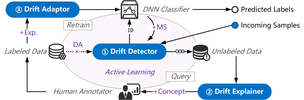
Figure 1: Active learning framework for concept drift mitigation: standard components and operations in common active learning (grey, italic), specialized components for concept drift (blue boxes), and new features of our method compared to existing works (purple).

3 Problem Setup

In this section, we define our research scope, formalize important components in the active learning-based strategy, and characterize current drift detectors with our formalization.

3.1 Research Scope

In this research, we adopt a proactive approach to addressing malware concept drift, employing active learning strategies that are in line with those used in CADE and HCC. The comprehensive process of this approach is depicted in Figure 1.

Distinguishing our method from HCC, we emphasize model-agnostic techniques, which are adept at operating effectively without modifications to the underlying classifier’s architecture. Recognizing that intra-class drift scenarios have already been extensively explored, our work primarily addresses the challenges associated with inter-class drifts. That is, we aim to delve deeply into the detection and adaptation strategies for drifts caused by unseen malware families. Nevertheless, it’s important to note that our proposed solution is not exclusively tailored to addressing inter-class drifts. The generalizability of our approach will also undergo a detailed evaluation in Section 7.

Our research setting bears a resemblance to that of CADE. However, we seek to further enhance the capabilities of both the drift detector and the drift explainer components. Another pivotal aspect of our work is addressing the unresolved issue of explanatory malware drift adaptation.

3.2 Formalization

Notations. We define an input instance $\mathbf{x}$ as an element of the feature space $\mathcal{X}\subseteq\mathbb{R}^{p\times q}$, where $p$ and $q$ represent dimensions pertinent to the attributes of the data. The label for any instance $\mathbf{x}$ is represented by $y$, where $y$ belongs to the label space $\mathcal{Y}$. The space $\mathcal{Y}$ can be binary, for instance, $\{0,1\}$ for malware detection tasks, or a finite set for malware classification, such as $\{1,2,\ldots,C\}$, with $C$ being the number of malware families. We consider two primary data partitions: the training dataset $\mathcal{D}_{\text{train}}$ used to train the predictive classifier, and the test dataset $\mathcal{D}_{\text{test}}$, employed for drift assessment. The classifier $\mathbf{M}$ functionally maps the feature space to the probability space over the labels, formalized as $\mathbf{M}:\mathcal{X}\rightarrow\mathcal{P}(\mathcal{Y})$, and the predicted label $\hat{y}$ for an instance $\mathbf{x}$ is the class with the highest probability, i.e., $\hat{y}=\operatorname*{argmax}_{y\in\mathcal{Y}}\mathbf{M}(\mathbf{x})[y]$.

Drift Detector. The drift detector, denoted by $\mathbf{D}$, is tasked with quantifying the extent of drift in the test dataset $\mathcal{D}_{\text{test}}$, with respect to the model $\mathbf{M}$ trained on $\mathcal{D}_{\text{train}}$. The detection process utilizes two main functions, i.e., uncertainty estimation function $unc:\mathcal{X}\times\mathbf{M}\rightarrow\mathbb{R}$ and nonconformity scoring function $ncm:\mathcal{X}\times\mathcal{Y}\times\mathcal{D}_{\text{train}}\rightarrow\mathbb{R}$.

The function $unc(\mathbf{x};\mathbf{M})$ represents the uncertainty estimation associated with $\mathbf{M}$ for an input instance $\mathbf{x}$, outputting an uncertainty metric to reflect the confidence of the predictive model. Concurrently, the nonconformity scoring function $ncm(\mathbf{x},\hat{y};\mathcal{D}_{\text{train}})=dis(\mathbf{x},sel(\hat{y},\mathcal{D}_{\text{train}}))$, which employs a specific distance measure to evaluate how much a new observation $(\mathbf{x},\hat{y})$ deviates from the calibration data selected from $\mathcal{D}_{\text{train}}$. Integrating these two measures, the drift detector $\mathbf{D}$ is defined by the following operation:

$$\mathbf{D}(\mathbf{x};\mathbf{M},\mathcal{D}_{\text{train}}):=agg(unc(\mathbf{x};\mathbf{M}),ncm(\mathbf{x},\hat{y};\mathcal{D}_{\text{train}})),$$ (1)

where $agg$ is a fusion function that combines the uncertainty and nonconformity scores into a singular drift metric. A higher output from $\mathbf{D}$ indicates a more pronounced drift, signaling the potential necessity for model adaptation.

Drift Explainer. The drift explainer, denoted by $\mathbf{E}$, elucidates the features that contribute to the transition from in-distribution (ID) data to out-of-distribution (OOD) data. For a given drifting sample $\mathbf{x}_{\text{drift}}$, the drift explainer seeks to learn a binary feature importance mask $\mathbf{m}\in\{0,1\}^{m\times n}$.

This involves a perturbation function, $per:(\mathbf{x},\mathbf{m})\mapsto\mathbf{x}^{\prime}$, that applies the mask $\mathbf{m}$ to the sample $\mathbf{x}_{\text{drift}}$, resulting in the perturbed sample $\mathbf{x}_{\text{drift}}^{\prime}$; a deviation function $dev:(\mathbf{x}^{\prime},\mathcal{D})\mapsto\mathbb{R}$ that quantifies the discrepancy between $\mathbf{x}_{\text{drift}}^{\prime}$ and the training data distribution $\mathcal{D}_{\text{train}}$. The optimization task is defined as:

$$\min_{\mathbf{m}}\left\{dev(per(\mathbf{x}_{\text{drift}},\mathbf{m}),\mathcal{D}_{\text{train}})+\alpha_{s}reg(\mathbf{m})\right\}.$$ (2)

In this formulation, $\alpha_{s}$ represents the regularization parameter promoting sparsity in the binary mask $\mathbf{m}$. The regularization function $reg$ might implement sparsity-inducing techniques such as the L1 norm or elastic-net [80]. The primary aim of this optimization is to minimize the deviation metric, ensuring that the positive values in the resulting mask $\mathbf{m}$ pinpoint the features driving the concept drift.

Drift Adaptor. The drift adaptor, denoted as $\mathbf{A}$, integrates the newly annotated data into the model updating process. It can be conceptualized as a function

$$\mathbf{A}:(\mathbf{x}_{\text{drift}},l_{\text{new}},\mathcal{D}_{\text{train}},\mathbf{M})\mapsto\mathbf{M}^{\prime}$$ (3)

that takes the new labels from the human annotator $l_{\text{new}}:=\mathbf{H}(\mathbf{x}_{\text{drift}})$, the original training dataset $\mathcal{D}_{\text{train}}$, and the current model $\mathbf{M}$, to update the model.

In this process, $\mathbf{A}$ first incorporates the annotated samples $(\mathbf{x}_{\text{drift}},l_{\text{new}})$ into the training dataset, resulting in an expanded dataset $\mathcal{D}_{\text{train}}^{\prime}$. Then, it retrains the model $\mathbf{M}$ using this updated dataset, yielding an adapted model $\mathbf{M}^{\prime}$. Specifically, in the scenario of inter-class drift, the role of $\mathbf{A}$ extends to updating the original label set $\mathcal{Y}$, accommodating new malware classes. This necessitates a modification in the model’s output layer to align with the updated label set $\mathcal{Y}^{\prime}$ before retraining.

3.3 Characterizing Current Drift Detectors

Current research in malware concept drift has predominantly concentrated on the development of effective detectors. In this section, we examine these detectors through the lens of our proposed formalization, categorizing them based on:

• Model sensitivity: the alignment of the drift detector with the specific characteristics of the classifier, which can lead to a more precise response to model-specific drifts.

• Data autonomy: the detector’s capability to operate independently of the training data during its operational phase, indicating adaptability and efficiency.

For DNNs, a straightforward uncertainty measurement ($unc$) is probability-based, typically using the negated maximum softmax output:

$$u_{0}(\mathbf{x};\mathbf{M}):=-\max_{y\in\mathcal{Y}}\mathbf{M}(\mathbf{x})[y].$$ (4)

In model-sensitive drift detectors, this uncertainty measure is incorporated into the drift scoring function using various approaches. The design of the nonconformity score ($ncm$) in current detectors all involves the utilization of the classifier’s training data during the testing phase. This includes comparing specific uncertainty values, establishing class centroids, or identifying the nearest neighbors in the latent space.

Transcendent Detector. In Transcendent’s drift detection approach, the nonconformity scoring ($ncm$) is implemented using p-values ($dis$) through a k-fold cross validation [67] approach ($sel$) . For a test instance $\mathbf{x}$, the p-value in a given fold is defined as the proportion of instances in the calibration set, which are predicted to be in the same class as $\mathbf{x}$ and have an uncertainty score at least as high as it: $\frac{|\{\alpha\in\mathcal{C}_{i}[\hat{y}_{i}]:u_{0}(\alpha;\mathbf{M}_{i})\geq u_{0}(\mathbf{x};\mathbf{M}_{i})\}|}{|\mathcal{C}_{i}[\hat{y}_{i}]|}$. Here, $\mathcal{C}_{i}\subset\mathcal{D}_{\text{train}}$ is the calibration set for the $i$-th fold in the k-fold partitioning, and $\mathbf{M}_{i}$ is the model retrained on the remaining training data $\mathcal{D}_{\text{train}}\setminus\mathcal{C}_{i}$. The function $u_{0}$ measures the model uncertainty of $\mathbf{M}_{i}$ for both the test instance $\mathbf{x}$ and each calibration instance in the class $\hat{y}_{i}=\mathbf{M}_{i}(\mathbf{x})$. In this case, the function $agg$ initially combines $unc$ implicitly in $ncm$ within each fold, and then aggregates these results across all folds with a median-like approach.

This method is characterized as semi model-sensitive as it involves retraining models $\mathbf{M}_{i}$ for each fold, instead of directly using the original classifier $\mathbf{M}$. It is highly dependent on the entire training dataset, as the test uncertainties are compared with each specific training point during calibrations.

CADE Detector. The CADE detector’s innovation lies in its distance function ($dis$), leveraging an autoencoder to map data from $\mathcal{X}$ into a latent space $\mathcal{Z}$ where inter-class relationships are captured. In this space, the selection function ($sel$) identifies class centroids as the average of latent vectors for each class: $\mathbf{c}_{y}=\mathbb{E}(\mathcal{Z}_{\text{train}}[y])$. The nonconformity measure ($ncm$) for a test instance $\mathbf{x}$ is then the minimum Euclidean distance from its latent representation $\mathbf{z}\in\mathcal{Z}$ to these class centroids $\{\mathbf{c}_{y};y\in\mathcal{Y}\}$. The autoencoder is trained with two loss items: the reconstruction loss to ensure the preservation of data integrity during encoding and decoding:

$$\mathcal{L}_{\text{rec}}=\mathbb{E}_{\mathbf{x}}\|\mathbf{x}-\hat{\mathbf{x}}\|_{2}^{2},$$ (5)

and the contrastive loss that minimizes distances between instances of the same class and enforces a margin $m$ between those of different classes:

$$\mathcal{L}_{\text{sep}}=\mathbb{E}_{\mathbf{x}_{i},\mathbf{x}_{j}}\left[\mathbb{I}_{y_{i}=y_{j}}d_{ij}^{2}+\sim\mathbb{I}_{y_{i}=y_{j}}\max(0,m-d_{ij})^{2}\right],$$ (6)

where $d_{ij}=\|\mathbf{z}_{i}-\mathbf{z}_{j}\|_{2}$ is the Euclidean distance between two latent representations, $\mathbb{I}_{y_{i}=y_{j}}$ is the binary indicator that equals $1$ for same-class pairs and $0$ for different-class pairs.

The CADE detector functions independently of the classifier, with both $unc$ and $agg$ not explicitly defined, resulting in a lack of model sensitivity. This aspect may be problematic in situations where model-specific drift detection is crucial for maintaining accuracy. On another note, this method is semi-independent of training data, which enhances the efficiency by relying on class centroids for drift detection rather than the entire dataset.

HCC Detector. Adapting the HCC detector for model-agnostic applications, the learning mechanism for the distance function ($dis$) closely resembles that of the CADE detector, except that: 1) the autoencoder’s decoder is replaced with a surrogate classifier $\mathbf{M}_{s}$ operating in the latent space; 2) the reconstruction loss is replaced with the binary cross-entropy loss $\mathcal{L}_{\text{ce}}$ of the surrogate classifier and the contrastive loss is adapted to a hierarchical form $\mathcal{L}_{\text{hc}}$, specific to intra-class drifts. For the selection function ($sel$), the HCC detector employs a nearest neighbor search in the training data. The final drifting score is calculated with a novel method, named pseudo loss, that uses the prediction label as the pseudo label for each test sample to calculate the losses:

$$\mathbf{D}_{\text{HCC}}(\mathbf{x};\mathcal{D}_{\text{train}})=\hat{\mathcal{L}}_{\text{ce}}(\mathbf{x};\mathbf{M}_{s})+\beta\hat{\mathcal{L}}_{\text{hc}}(\mathbf{x},\mathbf{x}_{j};\mathbf{x}_{j}\in\mathcal{N}(\mathbf{x})),$$ (7)

where $\mathcal{N}(\mathbf{x})\subseteq\mathcal{D}_{\text{train}}$ is the set of nearest neighbors of $\mathbf{x}$ in the latent space. The first item can be interpreted as a variation of $u_{0}(\mathbf{x};\mathbf{M}_{s})$ since the cross-entropy is also probability-based, and the second item is an implementation of $ncm$ restricted by class separation. Therefore, the $agg$ in this context is a weighted sum, with the weight given by the scalar $\beta$.

In this adapted context, the HCC detector exhibits semi model sensitive as it depends on the $unc$ derived from the surrogate classifier $\mathbf{M}_{s}$. Additionally, its operation is characterized by a reliance on the entire training dataset for identifying nearest neighbors.

4 Motivation and Challenge

	2016	2017	2018	2019	2020	Avg.
Prob.	0.631	0.646	0.600	0.696	0.662	0.647
Trans.	0.733	0.674	0.587	0.708	0.599	0.660
CADE	0.721	0.686	0.739	0.594	0.487	0.645
HCC	0.708	0.649	0.605	0.719	0.654	0.667
$\text{HCC}_{\text{ce}}$	0.711	0.649	0.606	0.719	0.655	0.668
$\text{HCC}_{\text{hc}}$	0.581	0.609	0.592	0.678	0.657	0.623

Table 2: Intra-class drift detection performance of existing works. For the state-of-the-art method HCC, we also make a separate study of the two items in its drift scoring function.

4.1 Lessons from Current Detectors

Despite the introduction of methods for drift detection in existing research, a comprehensive comparison focusing exclusively on their drift detection performance remains absent. This shortfall leads to a gap in understanding the true effectiveness of these methods under different conditions. Notably, the most recent work HCC has been recognized for its effectiveness in updating malware detection classifiers. This method is exclusively applicable to intra-class drifts. To address the gap, our study begins by examining the problem within an intra-class scenario. In the following, we establish a methodology for evaluating intra-class drift detection performance and provide several insights.

Evaluation Method. For malware detection tasks, we leverage malware samples from the Malradar dataset [69], which covers 4,410 malware across 180 families including singletons. Moreover, we make efforts to collect 43,641 benign samples in the same year period from 2015 to 2020. Our dataset has been carefully designed to mitigate spatial bias and temporal bias [50]. For the classifier, we use the Drebin features and an MLP model (detailed in Section 6.1). Regarding baselines, we take into account the vanilla probability-based detector (as depicted in Equation 4) and the three innovative detectors formalized in Section 3.3. During the evaluation phase, we assign positive drift labels to samples where predictions are incorrect, following the rationale that these misclassified samples are particularly valuable for adapting the classifier. This approach differs from inter-class drift detection, where positive drift labels are typically assigned based on the presence of unseen families, as utilized in existing work [75]. Then we compute the AUC metric using drifting scores and the ground truth drift labels.

Key Findings. Our evaluation results are shown in Table 2, from which we have identified four key findings. 1) The performance order in our experiments, i.e., HCC, Transcendent, and Probability all outperforming CADE, highlights the essential role of model sensitivity in effective drift detection. 2) Although CADE is not specifically tailored for intra-class drift, its superior performance in a non-model sensitive comparison with the $\text{HCC}_{hc}$ indicates the potential advantages of data autonomy and its autoencoder-based structure. 3) HCC surpassing Transcendent in performance indicates that learning a distance metric, rather than relying on calibration, can be more effective and efficient in complex models like DNNs. This observation contrasts with Transcendent’s findings on SVM models and is further supported by the efficiency of the detector’s training process, which can be up to 10 times faster. 4) The performance decline over time, particularly noticeable in the CADE method, suggests that continuous adaptation might be necessary not just for classifiers, but also for detection models.

4.2 Challenges in Human-in-the-loop

In the active learning framework utilized for drift adaptation, the involvement of human annotation presents specific challenges. The primary concern is the necessity to maintain a low human labeling budget, crucial due to the extensive efforts required in malware analysis [43]. The current adaptation approach, predominantly relying on retraining, is far from ideal in this context. This situation calls for a more refined technique that optimally utilizes human input while minimizing its extent, thereby achieving a balance between expert knowledge and resource constraints. Additionally, the potential for errors in human labeling, similar to inaccuracies observed in automated tools like antivirus scanners [71], underscores the need for resilience in the adaptation technique to mitigate labeling inconsistencies.

Furthermore, for effective human-computer collaboration in managing drift adaptation, it is critical that the system’s explanations of drift are intuitively understandable to humans. Current techniques, which often focus on feature attributions, can pose challenges in terms of intelligibility [62]. This alignment is essential for aiding humans in the labeling process, as it facilitates their understanding for malware labeling.

5 Our Dream System

We propose a system, named Dream, for drift detection and drift adaptation. In this section, we introduce design insights and technical details of the system.

5.1 Design Insights

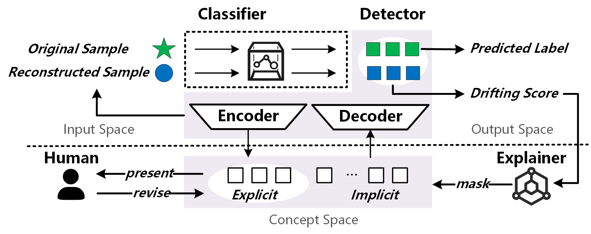
Figure 2: Design insights of Dream.

Building on the motivations and challenges, our design insights, as shown in Figure 2, propose innovative approaches for both drift detection and adaptation. For drift detection, we augment model sensitivity by utilizing classifier predictions on samples reconstructed by the detector. This enhancement is implemented by preserving the autoencoder structure within the CADE detector, allowing us to learn the distance metric and generate reconstructed samples, while integrating these with the classifier. Recognizing the need for data autonomy, especially in situations where training data is infeasible [53], the testing approach of our detector exclusively relies on the original sample, the reconstructed output, and the classifier’s probability outputs.

Addressing drift adaptation, we leverage latent representations to create a concept space reflective of malware behaviors, facilitating human intervention [61]. This approach not only employs annotated labels but also extends to the refinement of conceptual representations. By jointly refining both the classifier and the detector, we ensure a more nuanced capture of these evolving concepts. Furthermore, in alignment with the identified need for intuitive human-computer interaction, we have adapted our drift explainer to produce explanations within this concept space, thereby meeting human requirements for comprehensible revision.

5.2 Concept-based Drift Detection

Model Sensitive Concept Learning. We explore the idea of concept learning to enhance contrastive learning for latent representations in the drift detector. In the context of machine learning, concept learning typically involves the task of inferring boolean-valued functions from labeled examples to generalize specific instances to broader concepts [31, 16]. It is a form of supervised learning, where each concept, such as distinct geometric shapes (e.g., circles, squares, and triangles), is associated with a binary label for tasks like object identification [9]. Our intuition is that learning generalized concepts can offer a more direct method for identifying concept drift. To this end, we first define the concepts as malicious behaviors (e.g., information stealing, remote control, and stealthy download) under the malware context. Subsequently, our goal is to integrate the supervised concept learning with the unsupervised contrastive learning.

The contrastive autoencoder, denoted with $f$, produces reconstructed samples from given inputs, with the encoder $f_{\text{enc}}$ outputting latent representations and the decoder $f_{\text{dec}}$ operating on these representations for reconstruction. We define the unique latent space $\mathcal{Z}\subseteq\mathbb{R}^{N}$ in our method as the malware concept space, comprising the explicit concept space and the implicit concept space. Specifically, in the explicit concept space $\mathcal{Z}_{\text{exp}}$, each element $\mathbf{z}_{e}^{(i)}$ is structured to identify a distinct malicious behavior from a predefined collection. This approach mirrors traditional concept learning, where a boolean-valued function is employed to differentiate specific concepts. The implicit concept space $\mathcal{Z}_{\text{imp}}$ enriches the latent representations and plays a crucial role in refining the contrastive loss $\mathcal{L}_{\text{sep}}$. Firstly, given the overlapping nature of explicit behaviors across various malware families, it enhances the separation between classes within the concept space. Secondly, it allows for the expansion of behavior sets tailored to specific applications, including defining benign behaviors in binary malware detection tasks.

To further enhance the contrastive autoencoder-based drift detector, we introduce two key training requirements focused on concept handling. Firstly, we implement a concept presence loss for the precise detection of explicit concepts for each sample, which is defined as

$$\mathcal{L}_{\text{pre}}=-\mathbf{m}_{e}\odot\left(\mathbf{l}_{e}\odot\log(\mathbf{p}_{e})+(1-\mathbf{l}_{e})\odot\log(1-\mathbf{p}_{e})\right).$$ (8)

Here, $\odot$ denotes element-wise multiplication. The vectors $\mathbf{m}_{e}$, $\mathbf{l}_{e}$, and $\mathbf{p}_{e}$ each have a length of $N_{e}$, representing the total number of explicit concepts. The elements $\mathbf{m}_{e}^{(i)}$ and $\mathbf{l}_{e}^{(i)}$ correspond to the valid label mask and the binary label for the i-th concept, respectively; and $\mathbf{p}_{e}^{(i)}$ is calculated with $g(\mathbf{z}_{e}^{(i)})$, which is the probability of the i-th explicit concept being present. This formula aggregates binary cross-entropy for all explicit concepts, incorporating the valid label mask $\mathbf{m}_{e}$ to handle imprecise behavior labels. This strategy addresses the challenge of behavior labeling in the malware domain, where unlike the image domain with direct human annotations, concept labels often originate from technical reports or dynamic analysis and can be uncertain or missing [60].

Our second innovation is the introduction of the concept reliability loss, endowing the detector with model sensitivity from the early training stage. Our approach is based on the premise that a sample reconstructed from the concept space $\mathcal{Z}_{\text{exp}}\cup\mathcal{Z}_{\text{imp}}$ should exhibit a probability distribution similar to the original sample when processed by the classifier. The concept reliability loss is formally represented as

$$\mathcal{L}_{\text{rel}}=-\sum_{i}^{C}\mathbf{M}(\mathbf{x})^{(i)}\log(\mathbf{M}(\hat{\mathbf{x}})^{(i)}).$$ (9)

In this equation, the probability distributions of the original sample $\mathbf{x}$ serve as “true labels”, and those of the reconstructed sample $\hat{\mathbf{x}}$ are treated as predictions. This loss function effectively measures the divergence between the original and reconstructed sample distributions, ensuring that the model retains fidelity to the original concept representations even after reconstruction. Moreover, it implicitly measures the entropy-based uncertainty of the original distribution.

In summary, the training objective for our drift detector is centered on tuning the parameters of the autoencoder $f$ and the concept presence function $g$. This is achieved by minimizing the composite loss function over the training dataset, the concept labels, and the original classifier:

$$\mathcal{L}(\mathcal{D}_{\text{train}};\mathbf{l},\mathbf{M})=\lambda_{0}\mathcal{L}_{\text{rec}}+\lambda_{1}\mathcal{L}_{\text{sep}}+\lambda_{2}\mathcal{L}_{\text{pre}}+\lambda_{3}\mathcal{L}_{\text{rel}},$$ (10)

where the traditional reconstruction loss, the concept-based contrastive loss, the concept presence loss, and the concept reliability loss are balanced by coefficients $\lambda_{1}$, $\lambda_{2}$, and $\lambda_{3}$.

Concept Reliability Detector. With the trained detector, we can leverage it to detect drifting samples for incoming test data. Our design draws inspiration from a notable observation in the state-of-the-art HCC detector. Considering the significant contribution of the cross-entropy-based pseudo loss to the detection performance, we focus on enhancing the contrastive-based element in Equation 7. We firstly achieve this by maintaining the neighborhood function while substituting $\hat{\mathcal{L}}_{hc}$ with $\hat{\mathcal{L}}_{ce}$, leading to the introduction of the neighborhood cross-entropy (NCE) based pseudo loss, defined as

$$\mathbf{D}_{\text{nce}}(\mathbf{x;\mathcal{D}_{\text{train}}})=\hat{\mathcal{L}}_{\text{ce}}(\{\mathbf{x}\}\cup\mathcal{N}(\mathbf{x};f,\mathcal{D}_{\text{train}});\mathbf{M_{s}}).$$ (11)

In line with the experimental setup described in Section 4.1, we observe that this adjustment can improve the HCC detector’s performance to some extent: as shown in Table 3, the improvement in the average AUC achieves $6.11\%$.

	2016	2017	2018	2019	2020	Avg.
NCE	0.734 $\uparrow$$3.28$%	0.702 $\uparrow$$8.18$%	0.727 $\uparrow$$20.04$%	0.733 $\uparrow$$1.85$%	0.648 $\downarrow$$1.04$%	0.709 $\uparrow$$6.11$%

Table 3: The detection AUC of the proposed NCE compared with the original ce-based detector in HCC.

To comprehend the underlying principle, it’s important to understand that NCE calculates uncertainty for nearest neighbors based on the assumption that a non-drifting sample should remain certain even if slightly perturbed. This leads us to the samples reconstructed by the autoencoder, which essentially represent another type of perturbation. Consequently, the pseudo loss defined with our concept reliability loss (Equation 9) can align well with this principle. The drift scoring function of our detector is

$$u_{d}:=\mathbf{D}_{\textsc{Dream}}(\mathbf{x})=\hat{\mathcal{L}}_{\text{ce}}(\mathbf{x};\mathbf{M})+\lambda_{3}\hat{\mathcal{L}}_{\text{rel}}(\mathbf{x},f(\mathbf{x})),$$ (12)

where the first item is the pseudo cross-entropy loss of the test sample in terms of the original classifier, and the second can be interpreted as the deviation in uncertainty after meaningful perturbations. This approach can offer advantages for two primary reasons: 1) the perturbation $\hat{\mathbf{x}}=f(\mathbf{x})$ is confined within the meaningful concept space built with reconstruction requirements, and the loss calculation considers the entropy of both the original sample and the perturbation; 2) the testing phase of the detector is specifically designed for data autonomy, ensuring its efficiency and operational independence from the training data.

5.3 Explanatory Drift Adaptation

Explaining with Concept. To implement the two important functions ($per$ and $dev$) in the drift explainer, the existing CADE explainer leverages a reference sample from training data. This reference sample, denoted as $\mathbf{x}_{r}$, is selected from the latent space for its close representation of the class $y_{r}$, which is determined by the nearest class centroids to the drifting sample $\mathbf{x}_{d}$. The perturbation process involves using the mask $\mathbf{m}\in\mathbb{R}^{p\times q}$, resulting in the perturbed sample

$$\mathbf{x}_{d}^{\prime}:=\mathbf{x}_{d}\odot(1-\mathbf{m})+\mathbf{x}_{r}\odot\mathbf{m}\ .$$ (13)

The deviation is then quantified by calculating the distance between the latent representation of the perturbed sample, $\mathbf{z}_{d}^{\prime}$, and the nearest class centroid, represented as $d(\mathbf{z}_{d}^{\prime},\mathbf{c}_{y_{r}})$.

Motivated by this approach, our method focuses on generating concept-based explanations while leveraging the model-sensitive nature of our detector. First of all, in term of the selection of the nearest class $y_{r}$, we directly use $\hat{y}$ which is the class predicted by the original classifier. To create concept-based explanations, we introduce a concept-space mask $\mathbf{m}_{c}\in\mathbb{R}^{N}$. This mask redefines the perturbation function within the concept space, while still allowing us to compute the original distance-based deviation using latent representations. Further enhancing the deviation function, we incorporate the model-sensitive drifting scoring function. Therefore, the primary component of the explainer’s optimization function (Equation 2) is defined as

$$d\left(\mathbf{z}_{d}^{\prime},\mathbf{c}_{\hat{y}}\right)+\alpha_{u}\left(\hat{\mathcal{L}}_{\text{ce}}\left(\mathbf{x}_{d}^{\prime}\right)+\hat{\mathcal{L}}_{\text{rel}}\left(f\left(\mathbf{x}_{r}\right),\mathbf{x}_{d}^{\prime}\right)\right),$$ (14)

$$\operatorname*{s.t.}\mathbf{z}_{d}^{\prime}:=\mathbf{z}_{d}\odot(1-\mathbf{m}_{c})+\mathbf{z}_{r}\odot\mathbf{m}_{c},\ \mathbf{x}_{d}^{\prime}:=f_{\text{dec}}(\mathbf{z}_{d}^{\prime}),$$

where the the drifting score is balanced by $\alpha_{u}$ and determined by the feature-space perturbed sample $\mathbf{x}_{d}^{\prime}$ decoded from the perturbed concepts. Specifically in the pseudo concept reliability loss $\hat{\mathcal{L}}_{\text{rel}}$, the sample reconstructed from the reference input, i.e., $f(\mathbf{x}_{r})$, acts as a proxy for the true (or in-distribution) output probabilities. Note that our method can still generate feature-space explanations if needed. In that case, $\mathbf{x}_{d}^{\prime}$ is created with feature-space operations as in Equation 13, so that pseudo concept reliability loss will be in its typical form, which is $\hat{\mathcal{L}}_{\text{rel}}(\mathbf{x}_{d}^{\prime},f(\mathbf{x}_{d}^{\prime}))$.

Concept-involved Adaptor. Besides the drift explainer, our detector can serve as an explainer for in-distribution data in relation to the classifier. This is facilitated by the development of the explicit concept space. In this context, the outputs from the concept presence function $g$ are intrinsically linked to the malicious behaviors identified by the system. When dealing with out-of-distribution samples, it is possible that these explanations may be inaccurate due to the evolving nature of the concepts they are based on. Nevertheless, the architecture of our detector is designed to allow malware analysts to utilize the drift explainer as a tool and refine these behavioral concepts. This adaptable design is instrumental in updating and enhancing the classifier’s performance in response to conceptual drifts.

We enable human analysts to provide feedback not only on the predicted labels of drifting samples but also on their behavioral explanations. For instance, in malware classification tasks, analysts might encounter a drifting sample identified as belonging to the GhostCtrl family, exhibiting behaviors like PrivacyStealing, SMSCALL, RemoteControl, and Ransom. Feedback in this scenario could be formatted as: $$\begin{split}\exists mal\,\,\,\,&(\texttt{Family}(mal,\texttt{GhostCtrl}))\land(\texttt{Behaviors}(mal)\Leftrightarrow\\ &\texttt{PrivacyStealing}(mal)\land\texttt{SMSCALL}(mal)\\ &\land\texttt{RemoteControl}(mal)\land\texttt{Ransom}(mal)).\end{split}$$ The feedback can be generalized to identify specific malware families with minimal annotation effort, as in our experiments. An example of this is presented in Appendix C.

Utilizing the feedback provided, our drift adaptor operates by concurrently tuning the classifier and the detector. Let $\Theta$ represent the parameters of the classifier’s model, and $\Psi$ denote those of the detector. The optimization problem, which aims to minimize the combined loss functions of the classifier and the detector, is formally defined as

$$\min_{\{\Theta,\Psi\}}\left(\mathcal{L}_{\text{ce}(\Theta)}+\mathcal{L}_{\text{det}(\Psi)}+\lambda_{3}\mathcal{L}_{\text{rel}(\Theta,\Psi)}\right),$$ (15)

$$\operatorname{s.t.}\mathcal{L}_{\text{det}}=\lambda_{0}\mathcal{L}_{\text{rec}(\Psi)}+\lambda_{1}\mathcal{L}_{\text{sep}(\Psi)}+\lambda_{2}\mathcal{L}_{\text{pre}(\Psi)}.$$

The label feedback takes effect on the malware classification loss $\mathcal{L}_{\text{ce}}$ and the explanation feedback influences the concept presence loss $\mathcal{L}_{\text{pre}}$. Contrasting with the detector’s training process where $\Theta$ is fixed (Equation 12), during the adaptation phase, both $\Theta$ and $\Psi$ are subject to influence the concept reliability loss $\mathcal{L}_{\text{rel}}$. To address the complexities of joint parameter updating, we’ve implemented a dynamic learning rate schedule for the detector. Specifically, when $\mathcal{L}_{\text{det}}$ indicates concept stability—falling below a certain threshold—we reduce the learning rate using a scaling factor $\eta$. This reduction is based on the principle that stable concepts require less aggressive updates, promoting smoother model convergence and reducing the risk of overfitting.

6 System Evaluation

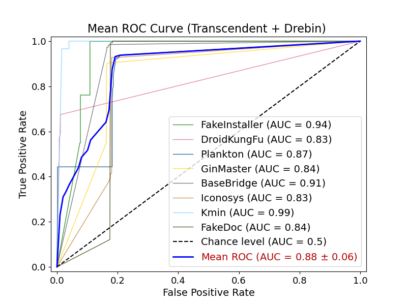
(a) Transcendent, Drebin

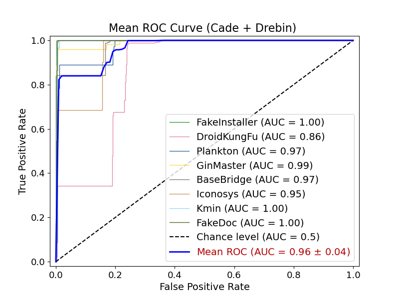
(b) CADE, Drebin

(c) Probability, Drebin

(d) (Ours) DREAM, Drebin

(e) Transcendent, Mamadroid

(f) CADE, Mamadroid

(g) Probability, Mamadroid

(h) (Ours) DREAM, Mamadroid

(i) Transcendent, Damd

(j) CADE, Damd

(k) Probability, Damd

(l) (Ours) DREAM, Damd

Figure 3: Evaluation of inter-class drift detection on Drebin dataset with three feature spaces. The first three columns are Transcendent, CADE, Probability, respectively, and our method is on the last column.

This section presents the evaluation of our system, specifically focusing on inter-class drift scenarios, which are central to our research. We systematically analyze each of the key components: drift detector, drift adaptor, and drift explainer.

6.1 Experimental Setup

Dataset. We employ two malware datasets for malware family classification tasks, as illustrated in Table 10. Our first dataset is the well-known Drebin dataset [4], adhering to the same criteria used in the CADE paper. To capture more recent trends in the evolving malware landscape, we utilize the Malradar dataset [69]. For each dataset, we select $8$ families, each comprising at least $100$ malware samples. The resulting datasets consist of $3,317$ and $2,589$ malware samples for Drebin and Malradar, respectively. Both datasets are well-labeled with respect to malware families. Additionally, Malradar provides behavioral labels derived from threat reports for each family, and we select $10$ distinct behaviors to form its behavioral labels. To ensure consistency in behavioral analysis, we augment the Drebin dataset with these same behaviors. Despite the simplicity, this approach is in line with an active learning setting that typically utilizes limited human effort. For more details about the two datasets, please also refer to Appendix B.

Classifier. We use three deep learning based malware classifiers, leveraging the features and models defined in previous works. These classifers differ in data modality and model complexity. 1) Drebin [4] classifier utilizes eight feature sets representing binary vectors of predefined patterns, such as required permissions and suspicious API calls. The underlying model is a MLP [22], configured with two hidden layers, sized at $100$ and $30$ neurons respectively. 2) Mamadroid [44] classifier involves extracting API call pairs and abstracting them into package call pairs. It builds a Markov chain to model the transitions between packages, using the derived float vectors as features. Its MLP architecture includes hidden layers with dimensions of $1,000$ and $200$. 3) Damd [47] classifier leverages the raw opcode sequences as features. The sequence representation utilizes an embedding technique with a vocabulary size of $218$ tokens and an embedding dimension of $128$. Its underlying model is a CNN tailored to this task, featuring two convolutional layers, each with $64$ filters.

Hold-out Strategy. To evaluate inter-class drifts, where the drift labels are determined based on whether a malware family was unseen during training, we employ a commonly used hold-out strategy [75, 60]. To implement this, we first exclude a select set of malware families from the training set, reserving them solely for the testing phase. The remaining families are then split in an 80:20 ratio for training and testing, adhering to a time-based separation criterion [65]. Through this strategy, $8$ classification models will be trained for each dataset, which is equal to the number of malware families.

Feature	Budget	Drebin Dataset						Malradar Dataset
		F1-score			Accuracy			F1-score			Accuracy
		w/o	w/	Imp.	w/o	w/	Imp.	w/o	w/	Imp.	w/o	w/	Imp.
Drebin	10	0.173	0.805	364.6%	0.168	0.778	363.1%	0.191	0.469	145.5%	0.207	0.525	153.9%
	20	0.528	0.928	75.7%	0.497	0.905	82.0%	0.291	0.921	216.8%	0.336	0.913	171.9%
	30	0.785	0.961	22.3%	0.744	0.952	28.0%	0.605	0.952	57.2%	0.629	0.948	50.8%
	40	0.886	0.956	7.9%	0.849	0.943	11.0%	0.631	0.967	53.3%	0.657	0.964	46.7%
	100	0.923	0.975	5.6%	0.901	0.973	8.0%	0.904	0.982	8.6%	0.892	0.981	10.0%
Mamadroid	10	0.169	0.648	282.9%	0.156	0.650	317.4%	0.476	0.651	36.8%	0.514	0.670	30.4%
	20	0.449	0.740	64.9%	0.435	0.736	69.3%	0.623	0.718	15.3%	0.626	0.725	15.9%
	30	0.601	0.789	31.4%	0.579	0.780	34.6%	0.718	0.734	2.3%	0.722	0.737	2.1%
	40	0.630	0.808	28.3%	0.621	0.794	27.8%	0.756	0.766	1.3%	0.747	0.759	1.5%
	100	0.814	0.864	6.2%	0.805	0.853	6.0%	0.821	0.839	2.2%	0.811	0.829	2.2%
Damd	10	0.442	0.738	66.9%	0.422	0.702	66.4%	0.246	0.525	113.7%	0.303	0.556	83.6%
	20	0.711	0.837	17.8%	0.684	0.820	19.9%	0.454	0.683	50.4%	0.497	0.707	42.1%
	30	0.775	0.849	9.5%	0.756	0.844	11.7%	0.681	0.750	10.2%	0.697	0.751	7.9%
	40	0.778	0.867	11.3%	0.766	0.863	12.7%	0.630	0.732	16.1%	0.669	0.749	11.9%
	100	0.888	0.955	7.59%	0.872	0.941	7.93%	0.768	0.811	5.5%	0.778	0.809	4.0%

Table 4: Drift adaptation results on two malware datasets within the three features.

Noise Ratio	F1-score			Accuracy
	w/o	w/	Imp.	w/o	w/	Imp.
0%	0.894	0.966	8.0%	0.863	0.956	10.7%
2%	0.862	0.950	10.2%	0.800	0.916	14.5%
6%	0.801	0.967	20.7%	0.760	0.976	28.4%
10%	0.822	0.945	14.9%	0.772	0.959	24.3%

Table 5: Drift adaptation under label noises with budget 50.

6.2 Drift Detection

Baseline and Metric. For assessing our drift detector’s performance in inter-class scenarios, we adopt the baseline methods previously utilized in the intra-drift detection, as outlined in Section 4.1. However, the HCC detector is excluded from this evaluation, considering its incompatibility with constructing hierarchical contrastive loss in these contexts. To ensure a fair comparison, both the CADE detector and our detector, which each leverage an autoencoder model, are configured to share the same architecture across all features (detailed in Appendix D). For the metric, we utilize the AUC calculated from the detector’s drifting score output and the ground truth labels, which are determined by the held-out malware families during the training process.

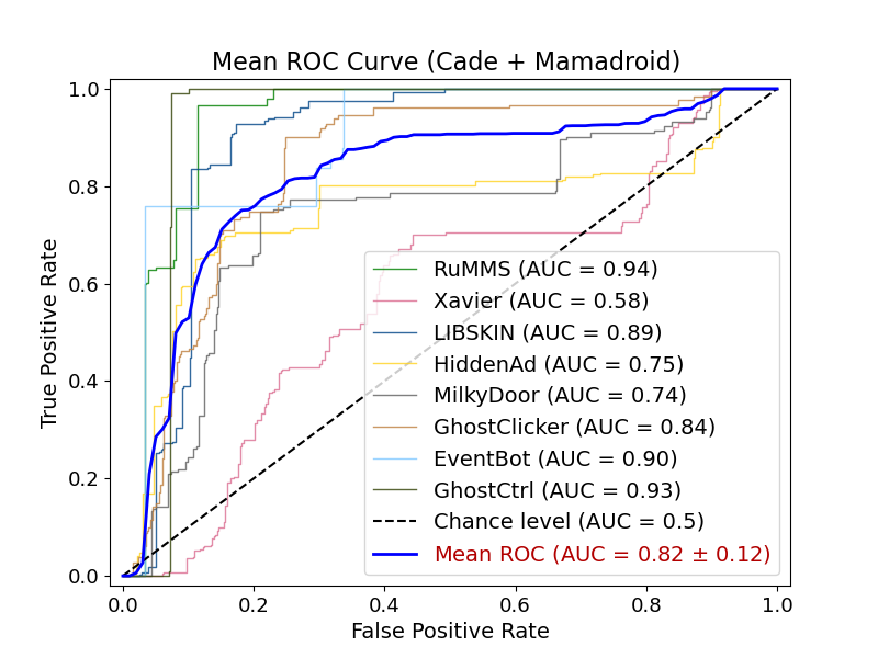
(e) CADE, Mamadroid

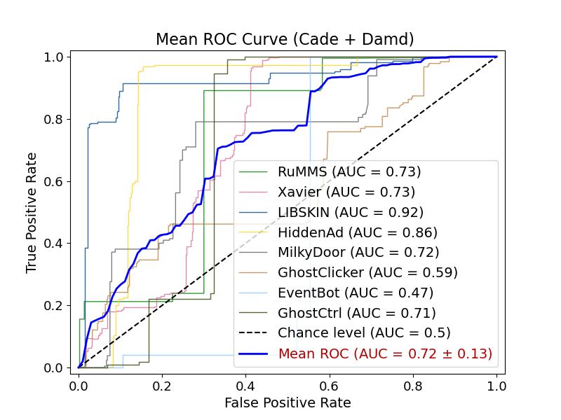
(f) CADE, Damd

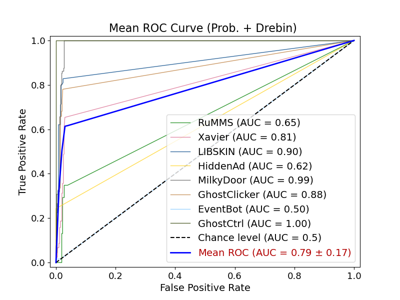
(g) Probability, Drebin

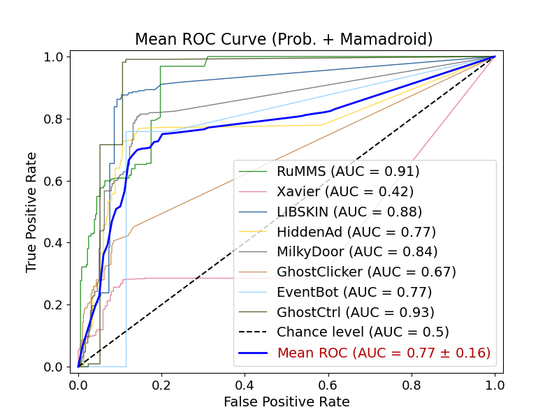
(h) Probability, Mamadroid

(i) Probability, Damd

(j) (Ours) DREAM, Drebin

(k) (Ours) DREAM, Mamadroid

(l) (Ours) DREAM, Damd

Figure 5: Evaluation of inter-class drift detection on Malradar dataset with three feature spaces. The first three rows are Transcendent, CADE, Probability, respectively, and our method is on the last row.

Evaluation Results. Figure 3 and Figure 5 depict the drift detection performance of our detector and the three baselines on the Drebin dataset and the Malradar dataset. Comparing the average AUC scores across different classifiers, We observe that Dream outperforms Transcendent, CADE, and Probability by 11.95%, 15.64%, and 12.4%, respectively, on the Drebin dataset. Similarly, on the Malradar dataset, Dream shows an increase of 10.98%, 8.33%, and 14.7%.

In evaluating detection performance for different classifiers, we observed three key points. For the Drebin classifier, which is simpler and where most methods excel, the CADE detector performs comparably to our method on both datasets. However, in classifiers with more complex feature spaces, CADE’s effectiveness can drop by 26.5%, while our method can show a 21.5% advantage. This highlights the importance of our model-sensitive property in handling model-specific drifts effectively. Regarding the Mamadroid classifier, it is less accurate in training compared to other classifiers. For this classifier, model-sensitive baselines such as Transcendent and Probability perform poorly. Our method, however, demonstrates stability and benefits from concept-based contrastive learning. In the case of the Damd classifier, the most complex among the tested, the Transcendent detector shows a smaller performance decline relative to other baselines. This is likely due to its calibration process, which boosts accuracy in scenarios of slight classifier overfitting (evidenced by a test accuracy of only 0.94, even 2.97% lower than that for the Mamadroid classifier). Although calibration proves beneficial, our method, with a focus on learning distance metrics, is more efficient, showing an average improvement of 6.62% over the Transcendent detector.

Explainer	Metric	f0	f1	f2	f3	f4	f5	f6	f7	Avg.
Random	CBP	0.239	0.145	0.131	0.070	0.093	0.191	0.225	0.057	0.144
	DRR	0.212	0.175	0.218	0.153	0.201	0.202	0.324	0.316	0.225
Dri-IG	CBP	0.154	0.217	0.166	0.246	0.103	0.194	0.299	0.208	0.198
	DRR	0.134	0.281	0.287	0.464	0.263	0.263	0.469	0.463	0.328
$\text{CADE}^{\text{+}}$	CBP	0.347	0.372	0.312	0.319	0.320	0.361	0.341	0.436	0.351
	DRR	0.834	0.722	0.781	0.791	0.788	0.752	0.808	0.819	0.787
Dream	CBP	0.348	0.408	0.331	0.402	0.338	0.372	0.487	0.443	0.391
	DRR	0.835	0.733	0.797	0.800	0.792	0.765	0.842	0.819	0.798

Table 6: Explanation evaluation results on the Drebin dataset with CBP and DRR metrics. The columns labeled f0 to f7 represent the held-out families, ordered by their sample size in descending order.

Explainer	CBP	DRR
Random	0.017 ± 0.031	0.023 ± 0.009
Dri-IG	0.228 ± 0.103	0.355 ± 0.337
CADE	0.173 ± 0.112	0.974 ± 0.009
Dream	0.331 ± 0.197	0.974 ± 0.009

Table 7: Evaluation of feature-level explanations.

6.3 Drift Adaptation

Baseline and Metric. We compare our adaptation methods against commonly used techniques that utilize selected samples and their annotated labels for classifier retraining [30, 14, 75]. Our experiments are conducted across a range of labeling budgets for active learning, specifically focusing on 10, 20, 30, 40, and 100, with an emphasis on smaller budgets to minimize the need for extensive human annotation. The effectiveness of each approach is quantified by measuring F1-scores and accuracy scores on the remaining test dataset. Additionally, we conduct a case study to assess the resilience of these methods against labeling noises, a common issue in practical applications [51]. This involves using the model trained on the Drebin feature of the Drebin dataset, with a fixed labeling budget of 50. For inter-class adaptation, an important step is the modification of the classifiers’ output layers to include new classes that were initially not part of the model. This modification involves randomly initializing the new output layer, while maintaining the previously learned weights in the existing layers. This approach ensures that the initial layers of the model continue to leverage the previously acquired knowledge, while the new output layer adapts to the newly introduced classes, and we adopt it consistently for each adaptation technique.

Evaluation Results. Table 4 shows the drift adaptation results across different labeling budgets on all datasets and classifiers. Our method outperforms the baseline in different settings without exception. Firstly, regarding performance improvements with different classifiers, we observed significant enhancements. On the Drebin dataset, the improvements are 82.0%, 69.3%, and 19.9% for Drebin, Mamadroid, and Damd classifiers, respectively. On the Malradar dataset, the improvements are even more pronounced at 171.9%, 15.9%, and 42.1% for the same classifiers.

Secondly, when considering varying human labeling budgets (10, 20, 30, 40, 100), the improvements on the Drebin dataset are 238.1%, 52.8%, 21.1%, 15.8%, and 6.5%, respectively. Similarly, on the Malradar dataset, the enhancements are 98.7%, 94.2%, 23.3%, 23.6%, and 5.5% for these respective budgets. A key finding is that the smaller the budget, the greater the improvement. This suggests that in scenarios prioritizing human analysis, our method can significantly reduces labeling budgets. For example, in order to achieve an accuracy score of 0.9 on the Drebin feature of the Drebin dataset, our method only needs 20 budgets, while the baseline requires 100, saving 80% of the analysis cost. On the Drebin feature of the Malradar dataset, the baseline method cannot achieve an accuracy score of 0.9 even if it uses 100 budgets, while our method can achieve an accuracy of 0.913 with the budget 20.

When considering the presence of labeling noise, the pivotal finding from Table 5 is that our method consistently achieves stable and higher F1-scores and accuracy scores compared to the baseline. Moreover, when the noise level increases, such as to 6%, the accuracy score improvement can reach 28.4%. This could be attributed to the inclusion of an explanation revision step during model updates, making our method more robust and resilient to noise.

6.4 Drift Explanation

Baseline and Metric. We consider three baseline methods for drift explanation, adapted to generate both concept-level and traditional feature-level explanations: 1) a random baseline that randomly selects features or concepts as important; 2) a gradient-based explainer that utilizes Integrated Gradients (IG) [63], adapted here to analyze drifting scores derived from our detector. Originally designed to attribute a deep network’s predictions to its input features, IG has demonstrated effectiveness in explicating supervised security applications [70, 27]. In this context, it is tailored to focus on the drifting scores derieved on model predictions, and the reference sample $\mathbf{x}_{r}$ serves as the baselines in its method; 3) the state-of-the-art CADE explainer used with the CADE detector, as described in Section 5.3. Since this method is not inherently designed for concept-space explanations, we adapt it to our detector for generating explanations in the concept space.

To evaluate the effectiveness of the drift explainers, we design two metrics. The first metric, named Cross Boundary P-value (CBP), assesses if explanations enable samples to cross the decision boundary, a key aspect in evaluating eXplainable AI (XAI) methods [57]. In our context, CBP is quantified as the proportion of training set samples with higher drifting scores than the perturbed samples, formally represented as:

$$\frac{|\{\alpha\in\mathcal{D}_{\text{train}}[\hat{y}_{i}]:u_{d}(\alpha;\mathbf{M})\geq u_{d}(\mathbf{x}_{d}^{\prime};\mathbf{M})\}|}{|\mathcal{D}_{\text{train}}[\hat{y}_{i}]|}.$$ (16)

The second metric, as suggested in existing research [75], focuses on the distance to the reference sample in the detector’s latent space after perturbation. We employ the Distance Reduction Rate (DRR) for this purpose, which measures the ratio of the reduced distance to the original distance between the drifting sample and the reference sample. It is worth mentioning that CBP is our primary metric of interest, as it directly correlates with classifier results, whereas DRR serves more as a supplementary measure in the latent space.

For a balanced comparison, particularly against the first two baseline methods that only yield importance scores, we align the number of altered features or concepts with those pinpointed by our techniques. These experiments are conducted using the Drebin feature of the Drebin dataset, maintaining consistency with the CADE paper’s approach, where the performance of its drift detector is established.

Evaluation Results. Table 6 illustrates the evaluation results of concept-based explanations generated by different methods. Comparing to three baseline explainers, i.e., Random, Dri-IG and $\text{CADE}^{\text{+}}$, Dream surpasses them by 172.1%, 97.2% and 11.5% on the CBP metric, and by 254.2%, 143.3% and 1.4% on the DRR metric. Notably, $\text{CADE}^{\text{+}}$ is included in this comparison as it utilizes our detector for concept-based explanations, extending beyond its original method’s capabilities. To examine the efficacy in areas typically addressed by common methods, Table 7 presents the outcomes for feature-level explanation evaluations. Here, our method, despite not being primarily designed for feature-level explanations, outperforms all baselines, including the state-of-the-art CADE explainer, benefiting from our method’s sensitive capture of deviations. Additionally, an intriguing observation is the contrast in CADE’s performance: its CBP value is 24.1% lower than that of Dri-IG, yet its DRR value is 61.9% higher. This discrepancy highlights the greater reliability of CBP over DRR in evaluating drift explainations. Combining the results from both tables, our explainer yields more substantial improvements in concept space than in feature space. For instance, while our method achieves a 45.2% increase in mean CBP over Dri-IG at the feature level, it shows a remarkable 97.2% increase at the concept level, highlighting the effectiveness of our design in concept space.

7 Extended Evaluation

In this evaluation stage, we expand our focus to examine the system’s effectiveness in detecting intra-class drifts, which is frequently emphasized in existing research.

Evaluation Method. In accordance with the evaluation practices in Section 4.1, we also extend the baselines by enhancing the HCC method with two specific adaptations: 1) the removal of the surrogate classifier $\mathbf{M}_{s}$ and its integration into the original classifier using the autoencoder structure; 2) the augmentation of the previous cross-entropy based pseudo loss item with our newly proposed NCE method, as in Equation 11. Theses modifications firstly render the HCC method fully model sensitive for detecting drift of external classifiers, and secondly make the uncertainty measurement more effective based on our observations in Section 5.2.

Evaluation Results. As presented in Table 8, our modification achieves significant enhancements in the HCC method’s detection performance. This is evident both in terms of the integrated method and its two individual pseudo-loss detectors. Notably, there is an average performance increase from $9.43\%$ to $10.62\%$. The contrastive-based pseudo-loss detector, previously the least effective, now surpasses all prior baselines with the most substantial improvement. This enhancement can be primarily attributed to the model-sensitive training approach. More importantly, our method demonstrates superior performance overall. Compared to existing methods, we achieve an $18.57\%$ improvement. Even when comparing against the improved HCC method, our approach maintains an $8.21\%$ lead. This superior performance is largely due to our unique approach in concept-based training and the data-autonomous design of our drift detection model.

	2016	2017	2018	2019	2020	Avg.
$\text{HCC}^{\text{+}}$	0.741 $\uparrow$$4.75$%	0.718 $\uparrow$$10.68$%	0.734 $\uparrow$$21.35$%	0.765 $\uparrow$$6.34$%	0.699 $\uparrow$$6.80$%	0.731 $\uparrow$$9.66$%
$\text{HCC}_{ce}^{\text{+}}$	0.745 $\uparrow$$4.84$%	0.724 $\uparrow$$11.52$%	0.719 $\uparrow$$18.74$%	0.768 $\uparrow$$6.81$%	0.698 $\uparrow$$6.63$%	0.731 $\uparrow$$9.43$%
$\text{HCC}_{hc}^{\text{+}}$	0.637 $\uparrow$$9.61$%	0.700 $\uparrow$$15.00$%	0.714 $\uparrow$$20.59$%	0.713 $\uparrow$$5.19$%	0.684 $\uparrow$$4.08$%	0.690 $\uparrow$$10.62$%
Dream	0.754 $\uparrow$$6.58$%	0.781 $\uparrow$$20.31$%	0.866 $\uparrow$$43.11$%	0.791 $\uparrow$$9.98$%	0.763 $\uparrow$$16.55$%	0.791 $\uparrow$$18.57$%

Table 8: The enhancement of intra-class drift detection with our detection framework.

8 Discussion

Below, we discuss potential avenues for future exploration.

Attack Surface. In the context of active learning, a notable security concern is the poisoning attacks, where adversaries introduce fake data to skew the retraining process [37]. Despite this, active learning has shown potential in mitigating such attacks in malware classifiers [46, 41]. Additionally, research has revealed the unexpected capability of an existing drift detector to detect adversarial malware samples [35]. While intentional attacks are beyond our current research scope, we show a similar resilience that Dream can handle noisy labels thanks to the explanatory design. Future work can be inspired to design new defense techniques.

Concepts and Annotators. We define malicious behaviors as concepts that effectively handles inter-class drift. To achieve comprehensive drift adaptation, we can explore border concepts. For example, the benign functionality can be included to better deal with intra-class drift. Furthermore, in the active learning framework, the human annotation step can be done in a more intelligent manner. Future efforts may utilize dynamic analysis tools [18, 1, 42] to automatically output behaviors or employ LLM models [10, 6] to generate higher-level contents.

9 Related Work

In this section, we discuss four additional areas of related work to complement Section 2.

OOD Detection. The majority of existing OOD detection methods in machine learning community rely on auxiliary OOD dataset [28, 11, 40, 45]. These datasets, composed of data points that are not part of the model’s training distribution, are used to train or fine-tune the model to better distinguish between ID and OOD samples. For instance, Chen et al. [11] uses an auxiliary dataset like the 80 Million Tiny Images. However, acquiring such large-scale and comprehensive auxiliary OOD datasets can be particularly challenging in the malware domain. Similar to existing work in malware domain, we are not dependent on auxiliary OOD dataset to offer greater practicality. Moreover, Dream operates independently of any training data during the drift detection phase, enhancing its applicability in real-world scenarios.

Labelless Drift Adaptation. In addition to human annotation strategy based on active learning, there is also drift adaptation strategy without labels [34]. For example, APIGraph [79] and AMDASE [73] use semantically-equivalent API usages to mitigate classifier aging [72]. However, they cannot be applied to classifiers that do not adopt API-based features [47], and API semantic analysis can be easily bypassed with obfuscation techniques [76, 59]. DroidEvolver [72, 34] employs pseudo-labels and is a promising solution to address labeling capacity. Nevertheless, this method can easily lead to negative feedback loops and self-poisoning [7]. Our work is based on active learning where labels can be provided with small analysis budgets, and these works can be complementary to us to further enhance the robustness in drift adaptation.

Explainable Security Applications. Recent research has focused on offering post-hoc explanations to security applications. For example, in malware detection [2, 4] tasks, FINER [27] produces function-level explanations to facilitate code analysis. In malware mutation [38, 12] applications, AIRS [77] explains deep reinforcement learning models in security by offering step-level explanations. On a different basis, Dream addresses the explainability problem in a drift adaptation setting, where the intrinsic behavioral explanations can propagate expert revisions to update the classifier.

Explanatory Interactive Learning. Recent advancements in machine learning have combined explainable AI with active learning, leading to progress in explanatory interactive learning [61, 58, 56]. Inspired by this, our approach incorporates human feedback on both labels and explanations, but with distinct objectives and settings. Unlike these works that focus on image domain and feature-level explanation annotation, our method is tailored for malware analysis and generates high-level explanations. Furthermore, while they use external explainers to guide classifiers away from artifacts [61], our approach integrates explanations directly within the drift detector, enhancing the efficiency of our drift adaptation method.

10 Conclusion

To deploy deep learning-based malware classifiers in dynamic and hostile environments, our work addresses a crucial aspect of combating concept drift. The proposed Dream system emerges as an innovative and effective solution, integrating model-sensitive drift detection with explanatory concept adaptation. The effectiveness of Dream against evolving threats is demonstrated through extensive evaluation and marks a notable advancement over existing methods. We hope that this work can inspire future research to explore concept drift in broader security contexts.

Appendix A Clarity of Notation

The notation in this paper is meticulously chosen and maintains consistency in the exposition of mathematical frameworks for malware concept drift handling. To ensure clarity, we adopt the following key formatting conventions:

• Sets are denoted with calligraphic script (e.g., $\mathcal{X},\mathcal{Y}$).

• Vectors and matrices are denoted by boldface letters to signify their multi-dimensional nature (e.g., $\mathbf{x}$).

• Scalars and elements of sets are represented in standard italicized font (e.g., $y,m,n$).

• Constant values, such as the number of malware families and the number of layers in a model, are represented as uppercase italicized characters (e.g., $C,K$).

• High-level functions, such as the predictive model $\mathbf{M}$, along with the Drift Detector $\mathbf{D}$, the Drift Explainer $\mathbf{E}$, and the Drift Adaptor $\mathbf{A}$, are denoted by boldface letters, emphasizing their functional significance.

• Lowercase three-letter abbreviations are reserved for unit functions within the primary processes (e.g., $unc$ for uncertainty estimation, $ncm$ for nonconformity scoring).

To facilitate reading, we list these symbols, as well as their descriptions and mappings in Table 9.

Symbol	Description and Mapping
$\mathcal{X},\mathbf{x}$	Feature space and an input instance
	$\mathcal{X}\subseteq\mathbb{R}^{p\times q},\mathbf{x}\in\mathcal{X}$
$\mathcal{Y},y$	Label space and the true label for $\mathbf{x}$
	$\mathcal{Y}:=\{0,1\}\text{ or }\{1,2,\ldots,C\},y\in\mathcal{Y}$
$\mathcal{D}_{\text{train}},\mathcal{D}_{\text{test}}$	Training and test datasets
	$\mathcal{D}_{\text{train}},\mathcal{D}_{\text{test}}\subseteq\mathcal{X}\times\mathcal{Y}$
$\mathbf{M}$	The target classifier
	$\mathbf{M}:\mathcal{X}\rightarrow\mathcal{P}(\mathcal{Y})$
$unc,ncm$	Uncertainty estimation and nonconformity scoring functions
	$unc:\mathcal{X}\times\mathbf{M}\rightarrow\mathbb{R}$, $ncm:\mathcal{X}\times\mathcal{Y}\times\mathcal{D}_{\text{train}}\rightarrow\mathbb{R}$
$\mathbf{D}$	Drift scoring function
	$\mathbf{D}:\mathcal{X}\times\mathcal{Y}\times\mathbf{M}\times\mathcal{D}_{\text{train}}\rightarrow\mathbb{R}$
$\mathbf{A}$	Model updating function
	$\mathbf{A}:\mathbf{M}\times\mathcal{D}_{\text{test}}\times\mathcal{E}\rightarrow\mathbf{M}^{\prime}$

Table 9: Notation table

Appendix B Malware Dataset

Family	# sample	(#) behavior	Time
FakeInstaller	925	$\text{(5) }\text{b}_{0}\text{, }\text{b}_{1}\text{, }\text{b}_{7}\text{, }\text{b}_{8}\text{, }\text{b}_{9}$	2011-2012
DroidKungFu	667	$\text{(3) }\text{b}_{0}\text{, }\text{b}_{2}\text{, }\text{b}_{6}$	2011-2012
Plankton	625	$\text{(4) }\text{b}_{0}\text{, }\text{b}_{2}\text{, }\text{b}_{7}\text{, }\text{b}_{8}$	2011-2012
GingerMaster	339	$\text{(2) }\text{b}_{0}\text{, }\text{b}_{6}$	2011-2012
BaseBridge	330	$\text{(4) }\text{b}_{0}\text{, }\text{b}_{1}\text{, }\text{b}_{6}\text{, }\text{b}_{9}$	2010-2011
Iconosys	152	$\text{(2) }\text{b}_{0}\text{, }\text{b}_{8}$	2010-2011
Kmin	147	$\text{(1) }\text{b}_{0}$	2010-2012
FakeDoc	132	$\text{(1) }\text{b}_{4}$	2011-2012

RuMMS	796	$\text{(4) }\text{b}_{0}\text{, }\text{b}_{1}\text{, }\text{b}_{2}\text{, }\text{b}_{3}$	2016-2018
Xavier	589	$\text{(4) }\text{b}_{0}\text{, }\text{b}_{2}\text{, }\text{b}_{7}\text{, }\text{b}_{8}$	2016-2021
LIBSKIN	290	$\text{(4) }\text{b}_{0}\text{, }\text{b}_{1}\text{, }\text{b}_{2}\text{, }\text{b}_{6}\text{, }\text{b}_{7}\text{, }\text{b}_{8}$	2015-2021
HiddenAd	289	$\text{(2) }\text{b}_{0}\text{, }\text{b}_{8}$	2017-2021
MilkyDoor	210	$\text{(2) }\text{b}_{0}\text{, }\text{b}_{2}$	2016-2020
GhostClicker	182	$\text{(4) }\text{b}_{0}\text{, }\text{b}_{2}\text{, }\text{b}_{6}\text{, }\text{b}_{8}$	2016-2020
EventBot	124	$\text{(5) }\text{b}_{0}\text{, }\text{b}_{1}\text{, }\text{b}_{2}\text{, }\text{b}_{3}\text{, }\text{b}_{5}$	2020
GhostCtrl	109	$\text{(3) }\text{b}_{0}\text{, }\text{b}_{1}\text{, }\text{b}_{2}$	2016-2020

Table 10: Drebin (top) and Malradar (bottom) datasets. In the third column, the number of existed behaviors is in parentheses, followed by their indices, with the specific meaning provided in Appendix B.

As shown in Table 10, we use two datasets for malware family classification. Specifically, we select 8 families for each of the Drebin [75] and the MalRadar [69] dataset, where the family selection adhers to the same criteria used in the CADE paper. The Drebin dataset spans the years from 2010 to 2012, offering insights into malware characteristics from ealy period. To capture more recent trends in the evolving malware landscape, the Malradar dataset [69] covers the period from 2015 to 2021.

We use the malicious behaviors defined in Malradar paper, where $\text{b}_{0}$-$\text{b}_{9}$ correspond to privacy information stealing ($\text{b}_{0}$), SMS/phone calls ($\text{b}_{1}$), remote control ($\text{b}_{2}$), bank stealing ($\text{b}_{3}$), ransom ($\text{b}_{4}$), abusing accessibility ($\text{b}_{5}$), privilege escalation ($\text{b}_{6}$), stealthy download ($\text{b}_{7}$), ads ($\text{b}_{8}$), and premium service ($\text{b}_{9}$). To ensure consistency in behavioral analysis, we augment the Drebin dataset, which originally lacks behavior labels, with these same behaviors. This extension involves extrapolating the labels based on Malradar’s definitions, supplemented by expert analysis and validation through GPT [48]. Note that the concept labels were assigned with minimal additional effort, and it is uniform within each family. In cases where certain behaviors in the Malradar dataset are specific to particular variants, we accommodate this by setting the relevant valid label mask $m_{e}$ to zero. Despite the simplicity, this approach is in line with an active learning setting that typically utilizes limited human effort.

For the Drebin dataset, the time-split is performed across all remaining families, as detailed in the CADE paper. For the Malradar dataset, its extensive time range and emergence of new families in recent years necessitate a tailored splitting approach. The previous split would classify newer families, such as EventBot which emerged in 2020, entirely into the testing set, potentially introducing unintended drift. To avoid this, we adjust the strategy by performing the split on a per-family basis within this dataset.

Appendix C High-level Human Feedback

The high-level abstraction of concept-based explanations allows feedback to be more generalized, potentially encompassing instances of a specific class and reducing the effort required for annotating explanations. An example of such generalized semantic feedback is: $$\begin{split}\forall mal\,\,\,\,&\texttt{Family}(mal,\texttt{GhostCtrl})\Rightarrow\\ &\texttt{Behaviors}(mal)\Rightarrow(\texttt{PrivacyStealing}(mal)\\ &\land\texttt{SMSCALL}(mal)\land\texttt{RemoteControl}(mal)),\end{split}$$ which implies that for all drifting samples in the GhostCtrl family, the expected behaviors include PrivacyStealing, SMSCALL, and RemoteControl, acknowledging that only some variants may exhibit the Ransom behavior.

Appendix D Autoencoder Architecture

For the Drebin feature, the autoencoder used is a form of Tabular Autoencoder consisting of two dense layers in both the encoder and decoder components. The architecture features a hidden dimension size of $512$ and an encoding dimension of $32$. In the case of the Mamadroid feature, the autoencoder is similarly structured as a Tabular Autoencoder, but with a larger hidden dimension of $2048$ and an encoding dimension of $128$. This expanded architecture accommodates the more complex nature of the Mamadroid feature set. For the Damd feature, the autoencoder is a specialized convolutional Text Autoencoder. This autoencoder works in conjunction with an embedding layer to facilitate reconstruction on numerical data. The encoder incorporates a convolutional layer with a kernel size of $3$ and $64$ filters, followed by a global max pooling layer. The decoder comprises a dense layer and a convolutional transpose layer that transform the data back into the embedding dimension, maintaining the same kernel size. This configuration is tailored to effectively handle the sequential nature of this feature set.

Appendix E Concept-based Explanation

The drift explainer in our system can explain OOD data, identifying concepts which contributes most to the drifting. As in Figure 4, we make an illustration of the drift explanations on the Drebin dataset.

Figure 4: The concept-based drift explanation heatmap on Drebin dataset, where the horizontal axis represents family names, and the vertical axis represents the proportion of explanation values that are positive for each behavior.

Hold-out	Baseline	Ours	Imp.
FakeInstaller	0.472	0.999	111.8%
DroidKungFu	0.496	1.000	101.8%
Plankton	0.516	1.000	93.9%
GingerMaster	0.526	1.000	90.2%
BaseBridge	0.527	1.000	89.8%
Iconosys	0.532	1.000	87.9%
Kmin	0.532	1.000	87.8%
FakeDoc	0.532	1.000	87.8%

Table 11: Concept classification accuracy for ID test data.

Besides drift explanation, our approach leverages an autoencoder intermediary to generate concept-based explanations, providing a novel tool for in-depth analysis of in-distribution data. The challenge in offering high-level explanations, beyond mere feature attribution, persists even in non-drifting scenarios. Current methodologies tend to abstract explanations from features [54, 27], but they cannot readily translate into behavioral insights.

To establish a baseline for concept-based explanations, we frame it as a series of binary classification tasks, each corresponding to a different explicit concept. Specifically, we adapt the output layer of the classifier to yield sigmoid probabilities and conduct fine-tuning over 100 retraining epochs. This ensures that each classifier achieves an accuracy of over 0.99 during training. We then select in-distribution data from the test dataset—specifically, data that corresponds to classes previously encountered during training—and assess the concept classification accuracy across all concepts.

We conduct the experiments with the Drebin dataset, and as detailed in Table 11, the results reveal that our method achieves near-perfect accuracy on the non-drifting test dataset, approaching $100\%$. This represents a significant $93.9\%$ improvement over the baseline across all models, indicating strong stability on in-distribution data. However, we observed a stark decrease in concept accuracy on out-of-distribution data, with average accuracies around $66\%$ for both the baseline and our method. Interestingly, the baseline shows a slight improvement in this context, possibly due to its conservative nature, leading to more frequent negative outputs. These ou emphasize the necessity of updating both the detector and classifier during drift adaptation, a key aspect of our drift adaptor’s design.

(a) Transcendent, Drebin

(b) Transcendent, Mamadroid

(c) Transcendent, Damd

(d) CADE, Drebin

References

- [1] Mohammed K Alzaylaee, Suleiman Y Yerima, and Sakir Sezer. Dynalog: An automated dynamic analysis framework for characterizing android applications. In 2016 International Conference On Cyber Security And Protection Of Digital Services (Cyber Security), pages 1–8. IEEE, 2016.
- [2] Hyrum S Anderson and Phil Roth. Ember: an open dataset for training static pe malware machine learning models. arXiv preprint arXiv:1804.04637, 2018.
- [3] Simone Aonzo, Yufei Han, Alessandro Mantovani, and Davide Balzarotti. Humans vs. machines in malware classification. In 32th USENIX Security Symposium (USENIX Security 23), 2023.
- [4] Daniel Arp, Michael Spreitzenbarth, Malte Hubner, Hugo Gascon, Konrad Rieck, and CERT Siemens. Drebin: Effective and explainable detection of android malware in your pocket. In Proceedings of the Network and Distributed Systems Security Symposium (NDSS), volume 14, pages 23–26, 2014.
- [5] Erin Avllazagaj, Ziyun Zhu, Leyla Bilge, Davide Balzarotti, and Tudor Dumitras. When malware changed its mind: An empirical study of variable program behaviors in the real world. In USENIX Security Symposium, pages 3487–3504, 2021.
- [6] Parikshit Bansal and Amit Sharma. Large language models as annotators: Enhancing generalization of nlp models at minimal cost. arXiv preprint arXiv:2306.15766, 2023.
- [7] Federico Barbero, Feargus Pendlebury, Fabio Pierazzi, and Lorenzo Cavallaro. Transcending transcend: Revisiting malware classification in the presence of concept drift. In 2022 IEEE Symposium on Security and Privacy (SP), pages 805–823. IEEE, 2022.
- [8] Jean Paul Barddal, Heitor Murilo Gomes, Fabrício Enembreck, and Bernhard Pfahringer. A survey on feature drift adaptation: Definition, benchmark, challenges and future directions. Journal of Systems and Software, 127:278–294, 2017.
- [9] Serge Belongie, Jitendra Malik, and Jan Puzicha. Shape matching and object recognition using shape contexts. IEEE transactions on pattern analysis and machine intelligence, 24(4):509–522, 2002.
- [10] Tianle Cai, Xuezhi Wang, Tengyu Ma, Xinyun Chen, and Denny Zhou. Large language models as tool makers. arXiv preprint arXiv:2305.17126, 2023.
- [11] Jiefeng Chen, Yixuan Li, Xi Wu, Yingyu Liang, and Somesh Jha. Robust out-of-distribution detection for neural networks. arXiv preprint arXiv:2003.09711, 2020.
- [12] Kai Chen, Peng Wang, Yeonjoon Lee, XiaoFeng Wang, Nan Zhang, Heqing Huang, Wei Zou, and Peng Liu. Finding unknown malice in 10 seconds: Mass vetting for new threats at the Google-Play scale. In 24th USENIX Security Symposium (USENIX Security 15), pages 659–674, 2015.
- [13] Ting Chen, Simon Kornblith, Mohammad Norouzi, and Geoffrey Hinton. A simple framework for contrastive learning of visual representations. In International conference on machine learning, pages 1597–1607. PMLR, 2020.
- [14] Yizheng Chen, Zhoujie Ding, and David Wagner. Continuous learning for android malware detection. arXiv preprint arXiv:2302.04332, 2023.
- [15] Zhi Chen, Zhenning Zhang, Zeliang Kan, Limin Yang, Jacopo Cortellazzi, Feargus Pendlebury, Fabio Pierazzi, Lorenzo Cavallaro, and Gang Wang. Is it overkill? analyzing feature-space concept drift in malware detectors. In 2023 IEEE Deep Learning Security and Privacy Workshop (DLSP). IEEE, 2023.
- [16] Thomas KF Chiu and Daniel Churchill. Design of learning objects for concept learning: Effects of multimedia learning principles and an instructional approach. Interactive Learning Environments, 24(6):1355–1370, 2016.
- [17] Theo Chow, Zeliang Kan, Lorenz Linhardt, Daniel Arp, Lorenzo Cavallaro, and Fabio Pierazzi. Drift forensics of malware classifiers. In Proc. of the ACM Workshop on Artificial Intelligence and Security (AISec). ACM, 2023.
- [18] Manuel Egele, Theodoor Scholte, Engin Kirda, and Christopher Kruegel. A survey on automated dynamic malware-analysis techniques and tools. ACM computing surveys (CSUR), 44(2):1–42, 2008.
- [19] Jerome Fan, Suneel Upadhye, and Andrew Worster. Understanding receiver operating characteristic (roc) curves. Canadian Journal of Emergency Medicine, 8(1):19–20, 2006.
- [20] Ming Fan, Jun Liu, Xiapu Luo, Kai Chen, Tianyi Chen, Zhenzhou Tian, Xiaodong Zhang, Qinghua Zheng, and Ting Liu. Frequent subgraph based familial classification of android malware. In 2016 IEEE 27th International Symposium on Software Reliability Engineering (ISSRE), pages 24–35. IEEE, 2016.
- [21] Liangyi Gong, Zhenhua Li, Feng Qian, Zifan Zhang, Qi Alfred Chen, Zhiyun Qian, Hao Lin, and Yunhao Liu. Experiences of landing machine learning onto market-scale mobile malware detection. In Proceedings of the Fifteenth European Conference on Computer Systems, pages 1–14, 2020.
- [22] Kathrin Grosse, Nicolas Papernot, Praveen Manoharan, Michael Backes, and Patrick McDaniel. Adversarial examples for detection. In Computer Security–ESORICS 2017: 22nd European Symposium on Research in Computer Security, Oslo, Norway, September 11-15, 2017, Proceedings, Part II 22, pages 62–79. Springer, 2017.
- [23] Alejandro Guerra-Manzanares, Marcin Luckner, and Hayretdin Bahsi. Concept drift and cross-device behavior: Challenges and implications for effective android malware detection. Computers & Security, 120:102757, 2022.
- [24] Wenbo Guo, Dongliang Mu, Jun Xu, Purui Su, Gang Wang, and Xinyu Xing. Lemna: Explaining deep learning based security applications. In Proceedings of the 2018 ACM SIGSAC Conference on Computer and Communications Security, pages 364–379, 2018.
- [25] Dongqi Han, Zhiliang Wang, Wenqi Chen, Kai Wang, Rui Yu, Su Wang, Han Zhang, Zhihua Wang, Minghui Jin, Jiahai Yang, et al. Anomaly detection in the open world: Normality shift detection, explanation, and adaptation. In Proceedings of the Network and Distributed Systems Security Symposium (NDSS), 2023.
- [26] Yiling He, Yiping Li, Lei Wu, Ziqi Yang, Kui Ren, and Zhan Qin. Msdroid: Identifying malicious snippets for android malware detection. IEEE Transactions on Dependable and Secure Computing, 20(3):2025–2039, 2023.
- [27] Yiling He, Jian Lou, Zhan Qin, and Kui Ren. Finer: Enhancing state-of-the-art classifiers with feature attribution to facilitate security analysis. In Proceedings of the 2023 ACM SIGSAC Conference on Computer and Communications Security, pages 416–430, 2023.
- [28] Dan Hendrycks and Kevin Gimpel. A baseline for detecting misclassified and out-of-distribution examples in neural networks. In International Conference on Learning Representations, 2016.
- [29] Wei-Ning Hsu and Hsuan-Tien Lin. Active learning by learning. In Proceedings of the AAAI Conference on Artificial Intelligence, volume 29, 2015.
- [30] Steve TK Jan, Qingying Hao, Tianrui Hu, Jiameng Pu, Sonal Oswal, Gang Wang, and Bimal Viswanath. Throwing darts in the dark? detecting bots with limited data using neural data augmentation. In 2020 IEEE symposium on security and privacy (SP), pages 1190–1206. IEEE, 2020.
- [31] Yangqing Jia, Joshua T Abbott, Joseph L Austerweil, Tom Griffiths, and Trevor Darrell. Visual concept learning: Combining machine vision and bayesian generalization on concept hierarchies. Advances in Neural Information Processing Systems, 26, 2013.
- [32] Yu Jiang, Ruixuan Li, Junwei Tang, Ali Davanian, and Heng Yin. Aomdroid: detecting obfuscation variants of android malware using transfer learning. In Security and Privacy in Communication Networks: 16th EAI International Conference, SecureComm 2020, Washington, DC, USA, October 21-23, 2020, Proceedings, Part II 16, pages 242–253. Springer, 2020.
- [33] Roberto Jordaney, Kumar Sharad, Santanu K Dash, Zhi Wang, Davide Papini, Ilia Nouretdinov, and Lorenzo Cavallaro. Transcend: Detecting concept drift in malware classification models. In 26th USENIX security symposium (USENIX security 17), pages 625–642, 2017.
- [34] Zeliang Kan, Feargus Pendlebury, Fabio Pierazzi, and Lorenzo Cavallaro. Investigating labelless drift adaptation for malware detection. In Proceedings of the 14th ACM Workshop on Artificial Intelligence and Security, pages 123–134, 2021.
- [35] KASTEL: Cryptography and Security Group. Detecting adversarial malware examples as concept drift, 2021. Accessed on November, 2023.
- [36] Igor Kononenko. Bayesian neural networks. Biological Cybernetics, 61(5):361–370, 1989.
- [37] Łukasz Korycki and Bartosz Krawczyk. Adversarial concept drift detection under poisoning attacks for robust data stream mining. Machine Learning, 112(10):4013–4048, 2023.
- [38] Balaji Lakshminarayanan, Alexander Pritzel, and Charles Blundell. Simple and scalable predictive uncertainty estimation using deep ensembles. Advances in neural information processing systems, 30, 2017.
- [39] Heng Li, Shiyao Zhou, Wei Yuan, Xiapu Luo, Cuiying Gao, and Shuiyan Chen. Robust android malware detection against adversarial example attacks. In Proceedings of the Web Conference 2021, pages 3603–3612, 2021.
- [40] Shiyu Liang, Yixuan Li, and Rayadurgam Srikant. Enhancing the reliability of out-of-distribution image detection in neural networks. arXiv preprint arXiv:1706.02690, 2017.
- [41] Jing Lin, Ryan Luley, and Kaiqi Xiong. Active learning under malicious mislabeling and poisoning attacks. In 2021 IEEE Global Communications Conference (GLOBECOM), pages 1–6. IEEE, 2021.
- [42] Davide Lorenzoli, Leonardo Mariani, and Mauro Pezzè. Automatic generation of software behavioral models. In Proceedings of the 30th international conference on Software engineering, pages 501–510, 2008.
- [43] Alessandro Mantovani, Simone Aonzo, Yanick Fratantonio, and Davide Balzarotti. Re-mind: a first look inside the mind of a reverse engineer. In Kevin R. B. Butler and Kurt Thomas, editors, 31st USENIX Security Symposium, USENIX Security 2022, Boston, MA, USA, August 10-12, 2022, pages 2727–2745. USENIX Association, 2022.
- [44] E Mariconti, L Onwuzurike, P Andriotis, E De Cristofaro, G Ross, and G Stringhini. Mamadroid: Detecting android malware by building markov chains of behavioral models. In Proceedings of the Network and Distributed Systems Security Symposium (NDSS), 2017.
- [45] Marc Masana, Idoia Ruiz, Joan Serrat, Joost van de Weijer, and Antonio M Lopez. Metric learning for novelty and anomaly detection. arXiv preprint arXiv:1808.05492, 2018.
- [46] Shae McFadden, Zeliang Kan, Lorenzo Cavallaro, and Fabio Pierazzi. Poster: Rpal-recovering malware classifiers from data poisoning using active learning. In Proc. of ACM Conference on Computer and Communications Security (CCS), 2023.
- [47] Niall McLaughlin, Jesus Martinez del Rincon, BooJoong Kang, Suleiman Yerima, Paul Miller, Sakir Sezer, Yeganeh Safaei, Erik Trickel, Ziming Zhao, Adam Doupé, et al. Deep android malware detection. In Proceedings of the seventh ACM on conference on data and application security and privacy, pages 301–308, 2017.
- [48] Yin Minn Pa Pa, Shunsuke Tanizaki, Tetsui Kou, Michel Van Eeten, Katsunari Yoshioka, and Tsutomu Matsumoto. An attacker’s dream? exploring the capabilities of chatgpt for developing. In Proceedings of the 16th Cyber Security Experimentation and Test Workshop, pages 10–18, 2023.
- [49] Tim Pearce, Alexandra Brintrup, and Jun Zhu. Understanding softmax confidence and uncertainty. arXiv preprint arXiv:2106.04972, 2021.
- [50] Feargus Pendlebury, Fabio Pierazzi, Roberto Jordaney, Johannes Kinder, and Lorenzo Cavallaro. Tesseract: Eliminating experimental bias in malware classification across space and time. In 28th USENIX Security Symposium (USENIX Security 19), pages 729–746, 2019.
- [51] Lukas Pirch, Alexander Warnecke, Christian Wressnegger, and Konrad Rieck. Tagvet: Vetting malware tags using explainable machine learning. In Proceedings of the 14th European Workshop on Systems Security, pages 34–40, 2021.
- [52] Dima Rabadi and Sin G Teo. Advanced windows methods on malware detection and classification. In Annual Computer Security Applications Conference, pages 54–68, 2020.
- [53] Pengcheng Ren, Chaoshun Zuo, Xiaofeng Liu, Wenrui Diao, Qingchuan Zhao, and Shanqing Guo. Demistify: Identifying on-device machine learning models stealing and reuse vulnerabilities in mobile apps. In 2024 IEEE/ACM 46th International Conference on Software Engineering (ICSE), pages 468–480. IEEE Computer Society, 2023.
- [54] Marco Tulio Ribeiro, Sameer Singh, and Carlos Guestrin. ‘why should i trust you?’ explaining the predictions of any classifier. In Proceedings of the 22nd ACM SIGKDD international conference on knowledge discovery and data mining, pages 1135–1144, 2016.
- [55] Jonathan C. Roberts, Panagiotis D. Ritsos, James R. Jackson, and Christopher Headleand. The explanatory visualization framework: An active learning framework for teaching creative computing using explanatory visualizations. IEEE Transactions on Visualization and Computer Graphics, 24(1):791–801, 2018.
- [56] Andrew Slavin Ross, Michael C Hughes, and Finale Doshi-Velez. Right for the right reasons: Training differentiable models by constraining their explanations. arXiv preprint arXiv:1703.03717, 2017.
- [57] Wojciech Samek, Alexander Binder, Grégoire Montavon, Sebastian Lapuschkin, and Klaus-Robert Müller. Evaluating the visualization of what a deep neural network has learned. IEEE transactions on neural networks and learning systems, 28(11):2660–2673, 2016.
- [58] Ramprasaath R Selvaraju, Stefan Lee, Yilin Shen, Hongxia Jin, Shalini Ghosh, Larry Heck, Dhruv Batra, and Devi Parikh. Taking a hint: Leveraging explanations to make vision and language models more grounded. In Proceedings of the IEEE/CVF international conference on computer vision, pages 2591–2600, 2019.
- [59] Jagsir Singh and Jaswinder Singh. Challenge of malware analysis: malware obfuscation techniques. International Journal of Information Security Science, 7(3):100–110, 2018.
- [60] Michael R Smith, Nicholas T Johnson, Joe B Ingram, Armida J Carbajal, Bridget I Haus, Eva Domschot, Ramyaa Ramyaa, Christopher C Lamb, Stephen J Verzi, and W Philip Kegelmeyer. Mind the gap: On bridging the semantic gap between machine learning and malware analysis. In Proceedings of the 13th ACM Workshop on Artificial Intelligence and Security, pages 49–60, 2020.
- [61] Wolfgang Stammer, Patrick Schramowski, and Kristian Kersting. Right for the right concept: Revising neuro-symbolic concepts by interacting with their explanations. In Proceedings of the IEEE/CVF conference on computer vision and pattern recognition, pages 3619–3629, 2021.
- [62] Zijun Sun, Chun Fan, Qinghong Han, Xiaofei Sun, Yuxian Meng, Fei Wu, and Jiwei Li. Self-explaining structures improve nlp models. arXiv preprint arXiv:2012.01786, 2020.
- [63] Mukund Sundararajan, Ankur Taly, and Qiqi Yan. Axiomatic attribution for deep networks. In International conference on machine learning, pages 3319–3328. PMLR, 2017.
- [64] Stefano Teso and Kristian Kersting. Explanatory interactive machine learning. In Proceedings of the 2019 AAAI/ACM Conference on AI, Ethics, and Society, pages 239–245, 2019.
- [65] Daniele Ucci, Leonardo Aniello, and Roberto Baldoni. Survey of machine learning techniques for analysis. Computers & Security, 81:123–147, 2019.
- [66] Joost Van Amersfoort, Lewis Smith, Yee Whye Teh, and Yarin Gal. Uncertainty estimation using a single deep deterministic neural network. In International conference on machine learning, pages 9690–9700. PMLR, 2020.
- [67] Vladimir Vovk. Cross-conformal predictors. Annals of Mathematics and Artificial Intelligence, 74:9–28, 2015.
- [68] Liu Wang, Ren He, Haoyu Wang, Pengcheng Xia, Yuanchun Li, Lei Wu, Yajin Zhou, Xiapu Luo, Yulei Sui, Yao Guo, et al. Beyond the virus: a first look at coronavirus-themed android malware. Empirical Software Engineering, 26(4):82, 2021.
- [69] Liu Wang, Haoyu Wang, Ren He, Ran Tao, Guozhu Meng, Xiapu Luo, and Xuanzhe Liu. Malradar: Demystifying android malware in the new era. Proceedings of the ACM on Measurement and Analysis of Computing Systems, 6(2):1–27, 2022.
- [70] Alexander Warnecke, Daniel Arp, Christian Wressnegger, and Konrad Rieck. Evaluating explanation methods for deep learning in security. In 2020 IEEE european symposium on security and privacy (EuroS&P), pages 158–174. IEEE, 2020.
- [71] Xian Wu, Wenbo Guo, Jia Yan, Baris Coskun, and Xinyu Xing. From grim reality to practical solution: Malware classification in real-world noise. In 2023 IEEE Symposium on Security and Privacy (SP), pages 2602–2619. IEEE Computer Society, 2023.
- [72] Ke Xu, Yingjiu Li, Robert Deng, Kai Chen, and Jiayun Xu. Droidevolver: Self-evolving android malware detection system. In 2019 IEEE European Symposium on Security and Privacy (EuroS&P), pages 47–62. IEEE, 2019.
- [73] Hongyu Yang, Youwei Wang, Liang Zhang, Xiang Cheng, and Ze Hu. A novel android malware detection method with api semantics extraction. Computers & Security, 137:103651, 2024.
- [74] Jingkang Yang, Kaiyang Zhou, Yixuan Li, and Ziwei Liu. Generalized out-of-distribution detection: A survey. arXiv preprint arXiv:2110.11334, 2021.
- [75] Limin Yang, Wenbo Guo, Qingying Hao, Arridhana Ciptadi, Ali Ahmadzadeh, Xinyu Xing, and Gang Wang. Cade: Detecting and explaining concept drift samples for security applications. In 30th USENIX Security Symposium (USENIX Security 21), 2021.
- [76] Ilsun You and Kangbin Yim. Malware obfuscation techniques: A brief survey. In 2010 International conference on broadband, wireless computing, communication and applications, pages 297–300. IEEE, 2010.
- [77] Jiahao Yu, Wenbo Guo, Qi Qin, Gang Wang, Ting Wang, and Xinyu Xing. AIRS: Explanation for deep reinforcement learning based security applications. In 32nd USENIX Security Symposium (USENIX Security 23), pages 7375–7392, 2023.
- [78] Shu Zhang, Ran Xu, Caiming Xiong, and Chetan Ramaiah. Use all the labels: A hierarchical multi-label contrastive learning framework. In Proceedings of the IEEE/CVF Conference on Computer Vision and Pattern Recognition, pages 16660–16669, 2022.
- [79] Xiaohan Zhang, Yuan Zhang, Ming Zhong, Daizong Ding, Yinzhi Cao, Yukun Zhang, Mi Zhang, and Min Yang. Enhancing state-of-the-art classifiers with api semantics to detect evolved android malware. In Proceedings of the 2020 ACM SIGSAC Conference on Computer and Communications Security, pages 757–770, 2020.
- [80] Hui Zou and Trevor Hastie. Regularization and variable selection via the elastic net. Journal of the Royal Statistical Society Series B: Statistical Methodology, 67(2):301–320, 2005.