Randomized iterative methods for generalized absolute value equations: Solvability and error bounds
Abstract.
Randomized iterative methods, such as the Kaczmarz method and its variants, have gained growing attention due to their simplicity and efficiency in solving large-scale linear systems. Meanwhile, absolute value equations (AVE) have attracted increasing interest due to their connection with the linear complementarity problem. In this paper, we investigate the application of randomized iterative methods to generalized AVE (GAVE). Our approach differs from most existing works in that we tackle GAVE with non-square coefficient matrices. We establish more comprehensive sufficient and necessary conditions for characterizing the solvability of GAVE and propose precise error bound conditions. Furthermore, we introduce a flexible and efficient randomized iterative algorithmic framework for solving GAVE, which employs sampling matrices drawn from user-specified distributions. This framework is capable of encompassing many well-known methods, including the Picard iteration method and the randomized Kaczmarz method. Leveraging our findings on solvability and error bounds, we establish both almost sure convergence and linear convergence rates for this versatile algorithmic framework. Finally, we present numerical examples to illustrate the advantages of the new algorithms.
1. Introduction
Absolute value equations (AVE) have recently become an active research area due to their relevance to many different fields, including the linear complementarity problem (LCP) [58], biometrics [15], game theory [77], etc. We consider the following generalized AVE (GAVE)
| (1) |
where , , and denotes the transpose. Specifically, when and is the identity matrix, the GAVE (1) reduces to the standard AVE [58]. When , the GAVE (1) becomes the system of linear equations. Over the past two decades, numerous works have examined the AVE problem from various perspectives, such as solvability [70, 71, 44, 30], error bounds [72], and the development of iterative methods [43, 2, 9, 10, 11, 60, 42]. While most of these works primarily focus on cases where , this paper, however, addresses the problem of non-square matrices.
In particular, we present a generic randomized iterative algorithmic framework for solving the GAVE (1). Starting from a proper , it iterates with the format
| (2) |
where is the stepsize, is a random matrix drawn from a user-defined probability space , and denotes the Euclidean norm. A typical case of the iteration scheme (2) is the randomized Kaczmarz (RK) method [63, 52]. For any , let denote the -th unit vector, denote the -th row of , and denote the -th entry of . Suppose that the coefficient matrix , the stepsize , and the sampling space with being sampled with probability . Then the iteration scheme (2) reduces to
which is exactly the RK method. See Section 5 for further discussion on the choice of the probability space for the recovery of existing methods and the development of new ones.
1.1. Our contribution
The main contributions of this work are as follows.
-
1.
We present a necessary and sufficient for the unique solvability of the GAVE (1); see Theorem 3.2. To the best of our knowledge, this is the first result to characterize the unique solvability of GAVE with non-square coefficient matrices. To improve the computational tractability of the proposed necessary and sufficient conditions, we further explore sufficient conditions that ensure the existence and uniqueness of the solution of GAVE. Different from the results in the literature, our conditions incorporate a nonsingular matrix, which makes our criteria more comprehensive; see Theorem 3.6, Corollary 3.9, and Theorem 3.11. In addition, we formulate a convex optimization problem to determine the existence of such nonsingular matrix.
-
2.
We establish error bounds for the GAVE (1), inspired by the recent work of Zamani and Hladík [72] on the standard AVE. Our results extend beyond the scope of their work. Not only do we propose error bounds for GAVE with non-square coefficient matrices, but our error bounds also incorporate a nonsingular matrix; see Theorem 3.16. It greatly generalizes and enhances the results in [72].
-
3.
We introduce a simple and versatile randomized iterative algorithmic framework for solving GAVE. Our general framework encompasses several known methods as special cases, including the Picard iteration method, the RK method, and its variants. This enables us to establish new connections between these methods. Additionally, the flexibility of our approach allows us to develop entirely new methods by adjusting the probability space . By leveraging the solvability and error bounds, we demonstrate both almost sure convergence and linear convergence for this general algorithmic framework. Finally, numerical examples illustrate the benefits of the new algorithms.
1.2. Related work
1.2.1. Solvability
Rohn [58] first introduced the alternative theorem for the unique solvability of the GAVE. This seminal work sparked a large amount of subsequent research exploring the unique solvability conditions of the GAVE [42, 44, 59, 60, 71, 69, 31]. One may refer to [36, 48] for recent surveys on the solvability of the GAVE. The unique solvability of GAVE is characterized by certain conditions derived from the analysis of the interval matrix, singular values, spectral radius, and norms of the matrices and involved in the equation. However, these conditions apply only when and are square matrices. In this paper, we delve into the unique solvability of the GAVE with non-square coefficient matrices. We establish more comprehensive conditions for characterizing the solvability of the GAVE, expanding the scope of previous research and providing a more inclusive understanding of the problem.
1.2.2. Error bound
Error bounds play a crucial role in theoretical and numerical analysis of linear algebraic and optimization [55, 76, 51, 27]. They provide a measure of the accuracy of an approximation, helping elucidate the stability and reliability of numerical methods and algorithms. In [66, 65], the authors established the numerical validation for solutions of standard AVE ( and ) based on the interval methods. Hladík [29] devised outer approximation techniques and derived an array of bounds for the solution set of the GAVE with square coefficient matrices. More recently, Zamani and Hladík [72] studied error bounds for standard AVE under the assumption that uniqueness of the solution of AVE is guaranteed. They then computed upper bounds for , i.e., the distance to the solution of the AVE, using a computable residual function. In this paper, we extend this line of research by proposing error bounds for GAVE with non-square coefficient matrices. Furthermore, our error bounds incorporate a nonsingular matrix, which significantly broadens and enriches the results presented in [72].
1.2.3. Existing methods for GAVE
In recent years, numerous algorithms have been developed to solve the GAVE with square coefficient matrices. Generally, these algorithms fall into four categories: Newton methods [12, 43, 8, 4, 23, 32], Picard iteration methods [60, 61, 11], splitting iteration method [35, 18, 11], and concave minimization approach [45, 1]. For some further comments, please refer to [2, 48]. Nevertheless, to our knowledge, there are merely two methods that can handle the GAVE with non-square coefficient matrices. The first is the successive linearization algorithm via concave minimization proposed in [42]. The second is the method of alternating projections (MAP) proposed in [2]. See sections 5 and 6 for more details and discussion of these methods. Our numerical results illustrate that, in comparison to these existing methods, our approach significantly outperforms in resolving non-square GAVE problems.
1.2.4. Stochastic algorithms
Stochastic algorithms, such as the RK method or the stochastic gradient descent (SGD) method [56], have gained popularity recently due to their small memory footprint and good theoretical guarantees [52, 63, 56]. The Kaczmarz method [34], also known as the algebraic reconstruction technique (ART) [26, 20], is a classical iterative algorithm used to solve the large-scale linear system of equations. The method alternates between choosing a row of the system and updating the solution based on the projection onto the hyperplane defined by that row. In the seminal paper [63], Strohmer and Vershynin studied the RK method and proved that if the linear system is consistent, then RK converges linearly in expectation. Since then, a large amount of work has been developed on Kaczmarz-type methods, including accelerated RK methods [37, 25, 39], randomized block Kaczmarz methods [50, 54, 53, 49, 22], greedy RK methods [3, 21], randomized sparse Kaczmarz methods [62, 13], etc.
In fact, the RK method can be seen as a variant of the SGD method [24, 52, 41, 74, 33]. The SGD method aims to minimize a separable objective function by stochastically accessing selected components of the objective and taking a gradient step for that component. That is, SGD employs the update rule
where is the step-size and is selected randomly. This approach allows SGD to make progress towards the minimum of the function using only a subset of the gradient information at each step, which can be computationally advantageous, especially for large-scale problems. When the objective function , then SGD reduces to the RK method. Furthermore, the randomized iterative method proposed in this paper can also be seen as an application of SGD. By incorporating information from the previous iteration, we formulate a stochastic optimization problem and then solve it by using a single-step of SGD; see section 4 for further discussion.
1.3. Organization
The remainder of the paper is organized as follows. After introducing some notations and preliminaries in Section , we study the solvability and error bounds in Section . In Section 4, we present the randomized iterative algorithmic framework for solving GAVE and establish its convergence. In Section 5, we mention that by selecting the probability space , the algorithmic framework can recover several existing methods as well as obtain new methods. In Section 6, we perform some numerical experiments to show the effectiveness of the proposed algorithms. Finally, we conclude the paper in Section 7.
2. Basic definitions and Preliminaries
2.1. Basic definitions
For any random variables and , we use and to denote the expectation of and the conditional expectation of given . For vector , we use , and to denote the -th entry, the transpose, and the Euclidean norm of , respectively. For , stands for the diagonal matrix whose entries on the diagonal are the components of .
Let and be matrices. We use , , , , , and to denote the -th component, the -th row, the transpose, the Moore-Penrose pseudoinverse, the Frobenius norm, and the column space of , respectively. If is nonsingular, then . The singular values of are . Given , the complementary set of is denoted by , i.e. . We use and to denote the row and column submatrix indexed by , respectively. The matrix inequality is understood entrywise and the interval matrix is defined as . We use to denote the identity matrix.
A symmetric matrix is said to be positive semidefinite if holds for any , and is positive definite if holds for any nonzero . We use to denote the eigenvalues of . We can see that , , and for any . Letting and denote the eigenvalue decomposition of , we denote with . For any two matrices and , we write () to represent is positive semidefinite (definite). For any , we define .
We use to denote the solution set of the GAVE (1). The generalized Jacobian matrices [14] are used in the presence of nonsmooth functions. Let be a locally Lipschitz function. The generalized Jacobian of at , denoted by , is defined as
where is the set of points at which is not differentiable and denotes the convex hull of a set . We use to denote the distance from to the set .
2.2. Some useful lemmas
In this subsection, we recall some known results that we will need later on. By the definition of singular value, we know that for any , . Therefore, we can conclude the following lemma.
Lemma 2.1.
Let and . Then for any , .
Lemma 2.2 ([75]).
Let . Then .
The following mean value theorem is useful for proving the error bound.
Lemma 2.3 ([28], Theorem ).
Let be a locally Lipschitz function on open subset of and let . Then there exist with , vectors , and matrices , such that
In order to proceed, we shall propose a basic assumption on the probability space used in this paper.
Assumption 2.1.
Let be the probability space from which the sampling matrices are drawn. We assume that is a positive definite matrix.
The following two lemmas are crucial for our convergence analysis.
Lemma 2.4 (Lemma 2.3, [40]).
Let be a real-valued random variable defined on a probability space . Suppose that is a positive definite matrix and with . Then
is well-defined and positive definite, here we define .
Lemma 2.5 ([67], Supermartingale convergence lemma).
Let and be sequences of nonnegative random variables such that a.s. for all , where denotes the collection . Then, converges to a random variable a.s. and .
3. Solvability and error bounds
3.1. Solvability
For the case where , Theorem 3.1 proposed by Wu and Shen [71] offers a characterization of the unique solvability of the GAVE (1).
Theorem 3.1 ([71], Theorem 3.2).
Suppose that . The GAVE (1) has a unique solution for any if and only if for any , the matrix is nonsingular.
For arbitrary values of and , the unique solvability of the GAVE (1) can be characterized by the following result, which can be viewed as a generalization of Theorem 3.1. To the best of our knowledge, this is the first result to characterize the unique solvability of GAVE with non-square coefficient matrices.
Theorem 3.2.
The GAVE (1) has a unique solution for any if and only if and for any , the matrix is nonsingular.
To prove Theorem 3.2, let us first prove a useful lemma. For any , we define the map as
| (3) |
We have the following conclusion for the map .
Lemma 3.3.
Suppose that . Then for any and , the map defined in (3) is not a bijection map.
Proof.
For the case where , we will prove that for any and , the map is not injective. Define , where . So in the first orthant, there exists a vector which satisfies . Since
we know that the null space of is non-empty. Note that lies in the interior of the first orthant, hence there exist infinitely many vector such that . This implies that the map is not injective.
For the case where , we will prove that for any and , the map is not surjective. For any , we define
where . Since
we have that the Lebesgue measure of is equal to zero. Thus,
which implies that the map is not surjective. ∎
Now, we are ready to prove Theorem 3.2.
Proof of Theorem 3.2.
For the case , based on the proof of Lemma 3.3, we can conclude the following result.
Corollary 3.4.
Suppose that . For any , there exist such that the GAVE (1) is unsolvable.
Corollary 3.4 implies that the GAVE (1) is generally unsolvable. The following theorem presents a necessary and sufficient condition for ensuring the solvability of the GAVE (1).
Theorem 3.5.
Proof.
The “If” part is obvious, so we focus on the “Only if” part. Since GAVE (1) is solvable, we know that there exist and such that and . Hence, ∎
If , Theorem 3.5 reduces to the fundamental result in linear algebra: the linear system is solvable (consistent) if and only if . However, checking the condition from Theorem 3.5 might not be easy. Therefore, a more efficiently computable condition is of interest. In the next subsection, we will investigate such conditions.
3.1.1. Sufficient conditions
Let us first consider the case where . We have the following result.
Theorem 3.6.
Suppose that and there exists a nonsingular matrix such that . Then for any , the GAVE (1) is solvable.
If , it is evident that a nonsingular matrix , for example , exists such that . Moreover, the following example indicates that even if , there might still exist a nonsingular matrix such that .
Example 3.7.
Let
We have and .
We note that there also exist matrices and , such as and , for which there is no matrix satisfying . Actually, for any given and , the existence of the matrix can be reformulated as a semidefinite programming (SDP) [64, 68], which will be further discussed in Section 3.1.2. Moreover, if a nonsingular matrix exists such that , Lemma 2.1 implies that satisfies , and for any , also satisfies . In other words, if there exists a matrix that satisfies , then there are multiple matrices that satisfy the same condition.
The following lemma is essential for proving Theorem 3.6.
Lemma 3.8.
Proof.
We can rewrite (1) as
| (4) |
It is follows from Theorem 3.1 that
has a unique solution, denoted as . Therefore, is a solution to (4), i.e., a solution to the GAVE (1). Hence, the GAVE (1) is solvable. If , Theorem 3.1 indicates that the GAVE (1) now has unique solution. On the other hand, if the GAVE (1) has unique solution for any , Theorem 3.2 ensures that . This completes the proof of this theorem. ∎
Now we are ready to prove Theorem 3.6.
Proof Theorem 3.6.
Suppose that there exists a such the GAVE (1) is unsolvable. By Lemma 3.8, we know that for every subset with , there exists a such that is singular. Then we have
where the last inequality follows from the Cauchy interlacing theorem. This contradicts to the assumption that . Hence, we know that the GAVE (1) is solvable for each . ∎
For the case , Theorem 3.6 can derive the following corollary.
Corollary 3.9.
Suppose that and there exists a nonsingular matrix such that . Then for any , the GAVE (1) has a unique solution.
Clearly, the condition in Corollary 3.9 is weaker than the condition provided in [70, Theorem 2.1]. If , Corollary 3.9 indicates that if , then for any , the GAVE (1) has a unique solution. Furthermore, the following example shows that even if , there exists a nonsingular matrix such that .
Example 3.10.
Let
We have and .
If , Corollary 3.4 implies that the GAVE (1) now is typically unsolvable. However, once it is solvable, the following result provides a sufficient condition to guarantee the uniqueness of the solution set .
Theorem 3.11.
Suppose that and is non-empty. If there exists a nonsingular matrix such that , then is singleton.
Proof.
Let , we have
Hence, . This completes the proof of this theorem. ∎
The following example considers that case where and , yet there exists a nonsingular matrix such that .
Example 3.12.
Let
We have and .
3.1.2. The existence of the matrix
In this subsection, we demonstrate that the problem of finding a nonsingular matrix such that can be reformulated as a convex optimization problem, where . For convenience, we assume that in the following discussion.
As discussed in Section 3.1.1, if a nonsingular matrix exists such that , then it holds that satisfies , and for any , also satisfies . Therefore, we only need to consider the constraint
to find a nonsingular matrix that satisfies . Besides, it can be verified that is a convex set.
For any given , we define as
Since for any fixed , is a convex function, and for any fixed , is a concave function; see [5, Section 3.2.3]. Hence, we have that is a convex function. Therefore, we can solve the convex optimization problem
| (5) |
to determine the existence of the nonsingular matrix . If is the optimal solution of (5) and , then is the desired nonsingular matrix such that
Otherwise, we know that there does not exist a nonsingular matrix that satisfies . We note that (5) is indeed a SDP, which can be solved efficiently.
3.2. Error bounds
Inspired by the recent work of Zamani and Hladík [72], this subsection investigates the error bounds for the solvable GAVE (1). In fact, based on the locally upper Lipschitzian property of polyhedral set-valued mappings as described in Proposition in [57], the GAVE (1) exhibits the local error bounds property. Specifically, there exist and such that when , it holds
| (6) |
However, in general, the global error bounds property does not hold necessarily, as demonstrated in Example in [72]. Next, we will provide several sufficient conditions under which the global error bounds property holds.
Theorem 3.13.
Let be non-empty. If zero is the unique solution of , then there exists such that
| (7) |
Proof.
The idea of the proof is similar to that of Theorem in [72] or Theorem 2.1 in [46]. Suppose to the contrary that (7) does not hold. Hence, for each , there exists such that
| (8) |
where . Due to the local error bounds property (6), there exists such that for each , where is sufficiently large. Consequently, tends to infinity as . Choosing subsequences if necessary, we may assume that goes to a non-zero vector . By dividing both sides of (8) by and taking the limit as goes to infinity, we get
which contradicts the assumptions. ∎
Corollary 3.9 and Theorem 3.11 have already provided sufficient conditions to guarantee that zero is the unique solution of . In addition to those results, the following proposition provides a simpler sufficient condition to ensure the uniqueness of the solution set of .
Proposition 3.14.
Suppose there exists an index such that . Then zero is the unique solution of .
Proof.
Based on the assumption, for any , it holds that if . Consequently, if , we have . Thus, if , we have . Therefore, zero is the unique solution of . ∎
To derive other types of error bounds, the following lemma is essential.
Lemma 3.15.
For any , there exists such that
Proof.
Theorem 3.16.
Suppose that is non-empty and for any , the matrix is full column rank. Then for any and nonsingular matrix ,
where represents any vector norm and its induced norm.
Proof.
From Lemma 3.15, we know that there exists a such that . Since is full column rank, we have
Thus
which completes the proof. ∎
Note that under the assumption of Theorem 3.16, it holds that . Assuming and if the matrix is full column rank (nonsingular) for every , Theorem 3.1 ensures a unique solution to the GAVE (1). Therefore, Theorem 3.16 yields the following corollary.
Corollary 3.17.
Assume that and is nonsingular for any . Then for any nonsingular matrix ,
where represents any vector norm and its induced norm.
If and , Corollary 3.17 recovers Theorem in [72], which provides an error bound for the standard system of AVE. Theorem 3.16 can also yield the following corollary.
Corollary 3.18.
Let be non-empty and is a nonsingular matrix. Suppose that and . Then
Proof.
For any , we have
Therefore, the matrix has full column rank, and thus, is also full column rank since is positive definite. Moreover, we have
Hence from Theorem 3.16, we have
as desired. ∎
4. Randomized iterative methods for GAVE
In this section, we present our randomized iterative method for solving the GAVE (1) and analyze its convergence properties. Randomization is incorporated into our method through a user-defined probability space that describes an ensemble of random matrices . The selection of the probability space should ideally be based on the specific problem at hand, as it can impact the error bounds and convergence rates of the method. Our approach and underlying theory accommodate a wide range of probability distributions; see Section 5 for further discussion.
At the -th iteration, we consider the following stochastic optimization problem
| (9) |
where with being a random variable in . Starting from , we employ only one step of the SGD method to solve the stochastic optimization problem (9)
where is drawn from the sample space and is the step-size. Particularly, we choose with . Now, we are ready to state the randomized iterative method for solving the GAVE (1) described in Algorithm 1.
-
1.
Randomly select a sampling matrix .
-
2.
Update
(10) -
3.
If a stopping rule is satisfied, stop and go to output. Otherwise, set and return to Step .
4.1. Convergence analysis
Let be any element of . For Algorithm 1, we establish the following convergence result. The parameters and are chosen to ensure that , which is a necessary condition for convergence.
Theorem 4.1.
Assume that is nonempty and the probability spaces satisfy Assumption 2.1. Let and be the iteration sequence generated by Algorithm 1.
-
(i)
If and , then at least one subsequence of converges a.s. to a point in the set and converges a.s. to zero.
-
(ii)
If and with , then is the unique solution and
-
(iii)
If zero is the unique solution of , with being given in Theorem 3.13, and with , then
Proof of Theorem 4.1.
For any , we have
where the inequality follows from and the last equality follows from the facts that and . Taking expectations, we have
| (11) | ||||
where the last inequality follows from the fact and . According to the supermartingale convergence lemma, converges a.s. for every . Thus, the sequence is bounded a.s., leading to the existence of accumulation points for . Furthermore, as a.s., it implies that a.s.. From Lemma 2.4, we know that is positive definite and hence a.s., i.e. a.s.. By the continuity of the function , for any accumulation point of , we have a.s.. This implies a.s..
Remark 4.2.
If , Theorem 4.1 aligns with the almost sure convergence result obtained through the properties of stochastic Quasi-Fejér sequences (see Remark 3.2 in [6]). Theorem 4.1 and can readily derive the almost sure convergence result. In fact, the proof of Theorem 4.1 reveals that Consequently, by applying the supermartingale convergence lemma (Lemma 2.5), we establish that a.s. Similarly, we can obtain that a.s. Furthermore, Theorem 4.1 and indicate Algorithm 1 exhibits the variance reduction property. In fact, supposing is bounded for all , by definition, we have
which implies that the convergence of leads to that of , namely, the reduction of variance.
5. Special cases: Examples
This section provides a brief discussion on the choice of the probability space in our method for recovering existing methods and developing new ones. While this list is not exhaustive, it serves to illustrate the flexibility of our algorithm.
5.1. The generalized Picard iteration method
When the sampling space , i.e. with probability one, and using the fact that , the iteration scheme (10) of our method becomes
| (13) |
In particular, when , and is nonsingular, the iteration scheme (13) recovers the Picard iteration method [60]. Hence, we refer to (13) as the generalized Picard iteration method.
In this case, the parameters in Theorem 4.1 can be simplified as , , and . If , then according to Theorem 4.1 , the iteration scheme (13) with has the following convergence property
The above convergence result recovers the result in [72, Proposition 22] when is nonsingular. We should note that the other convergence results in Theorem 4.1 still hold, although we have only illustrated the result mentioned above.
5.2. The gradient descent method
When the sampling space , i.e. with probability one, then the iteration scheme (10) of our method becomes
| (14) |
In particular, when , the iteration scheme (14) corresponds to the gradient descent method used to solve the least-squares problem.
In this case, the parameters in Theorem 4.1 can be simplified as , , and . If , then according to Theorem 4.1 , the iteration scheme (13) with exhibits the following convergence property
When , the above convergence property aligns with the convergence property of gradient descent for solving the least-squares problem, see e.g. [7, Theorem 3.10].
5.3. Randomized Kaczmarz method for GAVE
5.4. Randomized block Kaczmarz method for GAVE
When the sampling space , then the iteration scheme (10) of our method becomes
| (16) |
Particularly, when , the iteration scheme (16) corresponds to the randomized block Kaczmarz (RBK) method for solving linear systems [53]. We briefly review the strategies for selecting the subset for the RBK method [53, 19]. We define the number of blocks denoted by and divide the rows of the matrix into subsets, creating a partition . Then the block can be chosen from the partition using one of two strategies: it can be chosen randomly from the partition independently of all previous choices, or it can be sampled without replacement, which Needell and Tropp [53] found to be more effective. If , that is, if the number of blocks is equal to the number of rows, each block consists of a single row and we recover the RK method. The calculation of the pseudoinverse in each iteration is computationally expensive. However, if the submatrix is well-conditioned, we can use efficient algorithms like conjugate gradient for least-squares (CGLS) to calculate it.
To analyze the convergence of the RBK method, it is necessary to define specific quantities [53]. The row paving of a matrix is a partition that satisfies
where indicates the size of the paving, and and denote the lower and upper paving bounds, respectively. Assume that is a matrix with full column rank and row paving , and the index is selected with probability . Let us now consider the parameters in Theorem 4.1. The parameter satisfies , and consequently, , and . If , then according to Theorem 4.1 , the iteration scheme (16) with exhibits the following convergence property
When , this convergence property aligns with that of the RBK method for solving consistent linear systems with full column rank coefficient matrices, as detailed in [53, Theorem 1.2].
In practice, the RBK method may encounter several challenges, including the computational expense at each iteration due to the necessity of applying the pseudoinverse to a vector, which is equivalent to solving a least-squares problem. Additionally, the method presents difficulties in parallelization. To overcome these obstacles, the randomized average block Kaczmarz (RABK) method was introduced [50, 49, 17, 73].
5.5. Randomized average block Kaczmarz method for GAVE
The randomized average block Kaczmarz (RABK) method is a block-parallel approach that computes multiple updates at each iteration [50, 49, 17, 73]. Specifically, consider the following partition of
where is a uniform random permutation on and is the block size. We define and select an index with the probability , and then set . The iteration scheme (10) of our method becomes
| (17) |
Particularly, when , the iteration scheme (17) corresponds to the randomized average block Kaczmarz (RABK) method for solving linear systems [50, 17, 49, 73].
In this case, the parameters in Theorem 4.1 can be simplified as , , and . If , then according to Theorem 4.1 , the iteration scheme (13) with exhibits the following convergence property
If , meaning that each block only contains a single row, then the iterative scheme (17) recovers the RK method (15) for GAVE, and the convergence result stated above aligns with the result established in Section 5.3.
We now make a comparison between the cases where and . For convenience, we assume that . The convergence factors for the cases and are and , respectively. Since the computational cost for the case at each step is about -times as expensive as that for the case , we can turn this comparison into a comparison between and . Since , it follows that
This suggests that, theoretically, the RABK method with is more efficient than the RABK method with for solving the GAVE (1). However, we note that one can use the parallelization technique to speed-up the iteration scheme (17) in terms of the total running time.
Finally, we note that the versatility of our framework and the general convergence theorem (Theorem 4.1) allow for the adaptation of the probability spaces to suit specific problems. For instance, random sparse matrices or sparse Rademacher matrices could be particularly appropriate for certain classes of problems.
6. Numerical experiments
In this section, we study the computational behavior of the proposed randomized iterative method. In particular, we focus mainly on the evaluation of the performance of the RABK method for GAVE. We compare RABK with some of the state-of-the-art methods, namely, the generalized Newton method (GNM) [43, 32], the Picard iteration method (PIM) [60], the successive linearization algorithm (SLA) [42], and the method of alternating projections (MAP) [2].
All the methods are implemented in MATLAB R2022a for Windows on a desktop PC with Intel(R) Core(TM) i7-1360P CPU @ 2.20GHz and 32 GB memory. The code to reproduce our results can be found at https://github.com/xiejx-math/GAVE-codes.
We have previously detailed the PIM in Section 5.1. Next, we briefly describe GNM, SLA, and MAP, respectively.
-
(i)
Generalized Newton method (GNM) [43, 32]. This algorithm is aimed at solving the GAVE (1) with and the iterations are given by
where . The iterations are derived by applying the semismooth Newton method in solving the equation . As in [43], we use the MATLAB’s backslash operator “\” to obtain the iterates.
- (ii)
-
(iii)
Method of alternating projections (MAP) [2]. Let and consider the following feasibility problem
(19) where
and
In [2], the authors showed that the GAVE (1) is equivalent to the feasibility problem (19), i.e., if solves (19), then solves the GAVE (1). The method of alternating projections (MAP) can be employed to solve (19). Particularly, starting from a proper , the MAP iterates with the format
Here for any , we have
and if and only if for each ,
For the case , we compare our algorithm with GNM, PIM, and MAP. We exclude the SLA from this comparison due to its extensive computational time demands when addressing these problems. In the more general case, our algorithm is compared solely with the SLA and the MAP. This is because the other solvers, namely GNM and PIM, are only capable of handling square matrices. All computations are initialized with . The computations are terminated once the relative solution error (RSE), defined as , or the relative residual error (RRE), defined as , is less than a specific error tolerance. For the RABK method, we set and for the SLA, we set . All the results below are averaged over trials.
6.1. Synthetic data
The coefficient matrices are randomly Gaussian matrices generated by the MATLAB function randn. Letting , we initially construct a matrix and subsequently construct such that , where , , and . Here, is a diagonal matrix and . Using MATLAB notation, these matrices are generated by the following commands: B=randn(m,n) or B=eye(n), [U,]=qr(randn(m,r),0), [V,]=qr(randn(n,r),0), and P=norm(B)*eye(r)+diag(rand(r,1)). We generate the exact solution by and then set . In this example, . Therefore, the GAVE (1) has a unique solution if (see Corollary 3.9 and Theorem 3.11). The computations are terminated once the RSE is less than .
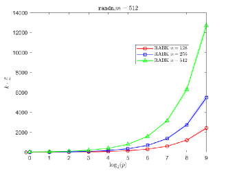
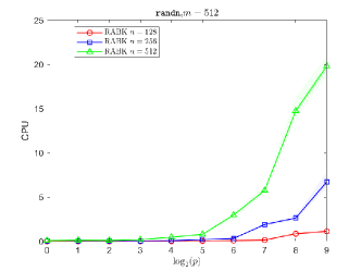
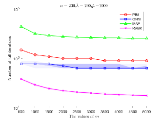
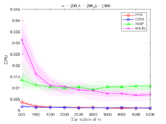
First, we explore the influence of the block size on the convergence of the RABK method in solving the GAVE (1) with randomly generated Gaussian matrices. The performance of the algorithms is measured in both the computing time (CPU) and the number of full iterations , which makes the number of operations for one pass through the rows of are the same for all the algorithms. In this experiment, we fix and set to be , and . The results are displayed in Figure 1. The bold line illustrates the median value derived from trials. The lightly shaded area signifies the range from the minimum to the maximum values, while the darker shaded one indicates the data lying between the -th and -th quantiles. From Figure 1, it can be seen that as the value of increases, both the CPU time used by the algorithm and the number of full iterations increase. This indicates that the smaller the value of , the better the performance of the RABK method, which is consistent with the discussion in Section 5.5. Therefore, in the subsequent tests, we take .
|
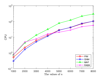
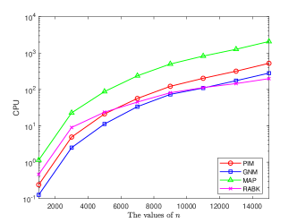
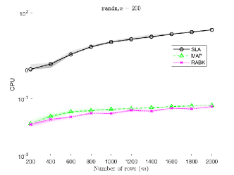
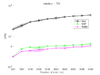
In Figure 2, we report the averages CPU times for PIM, GNM, MAP, and RABK when using square coefficient matrices, i.e., . From Figure 2, it can be observed that when is relatively small, the GNM outperforms the other methods, with RABK and PIM being the least efficient. However, as increases, the performance of the RABK method gradually improves, eventually surpassing the other algorithms and emerging as the most efficient method. Figure 3 compares the SLA, MAP, and RABK methods when employing non-square coefficient matrices. The results demonstrate that the RABK method outperforms both SLA and MAP.
|
|
6.2. Ridge Regression
Ridge regression is a popular parameter estimation method used to address the collinearity problem frequently arising in multiple linear regression [47, 16]. We consider an asymmetric ridge regression of the form:
where the penalty parameters and satisfy . We note that the case for every corresponds to the classical ridge regression, which will not be considered here. The case for all and corresponds to a penalization of the negativity of the coefficients, promoting solutions with positive coefficients. The necessary condition for optimality is given by:
where denotes the componentwise (or Hadamard) product. Noting that and , we end up with the following problem
| (20) |
If we set and for every and consider the loss function , where and . Then (20) becomes the following GAVE problem
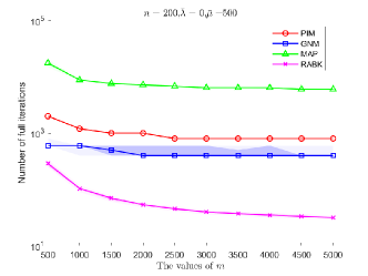
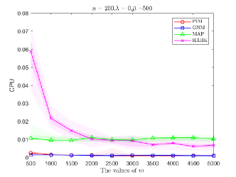
Figure 4 illustrates our experimental results for varying values of , and . The matrix and vector are randomly generated with values in . The computations are terminated once the RRE is less than and set for the RABK method. The performance of the algorithms is measured in the computing time (CPU) and the number of full iterations. From the iteration schemes of PIM, GNM, and MAP, it can be seen that one iteration of PIM and GNM corresponds to one full iteration, while one iteration of MAP corresponds to two full iterations. It can be observed from Figure 4 that RABK outperforms the other methods in terms of the number of full iterations. However, in terms of CPU time, both PIM and GNM outperform RABK, even though we only show the CPU time taken by RABK to execute (17). This is because the parallel processing capability of MATLAB can help alleviate the computational costs associated with computing the inverse of a matrix.
|
|
7. Concluding remarks
We have proposed a simple and versatile randomized iterative algorithmic framework for solving GAVE, applicable to both square and non-square coefficient matrices. By manipulating the probability spaces, our algorithmic framework can recover a wide range of popular algorithms, including the PIM and the RK method. The flexibility of our approach also enables us to modify the parameter matrices to create entirely new methods tailored to specific problems. We have provided conditions that ensure the unique solvability and established error bounds for GAVE. Numerical results confirm the efficiency of our proposed method.
This work not only broadens the applicability of randomized iterative methods, but it also opens up new possibilities for further algorithmic innovations for GAVE. The momentum acceleration technique, a strategy recognized for its effectiveness in enhancing the performance of optimization methods [24, 39, 73], presents a promising area of exploration. Investigating a momentum variant of randomized iterative methods for the GAVE problem could yield significant advancements in this field. Moreover, real-world applications often present challenges in the form of uncertainty or noise in the input data or computation. Inexact algorithms have been recognized for their ability to provide robustness and flexibility in handling such uncertainties [11, 38]. Analyzing inexact variants of randomized iterative methods for solving GAVE would also be a valuable topic.
References
- [1] Lina Abdallah, Mounir Haddou, and Tangi Migot. Solving absolute value equation using complementarity and smoothing functions. Journal of Computational and Applied Mathematics, 327:196–207, 2018.
- [2] Jan Harold Alcantara, Jein-Shan Chen, and Matthew K Tam. Method of alternating projections for the general absolute value equation. Journal of Fixed Point Theory and Applications, 25(1):39, 2023.
- [3] Zhong-Zhi Bai and Wen-Ting Wu. On greedy randomized Kaczmarz method for solving large sparse linear systems. SIAM J. Sci. Comput., 40(1):A592–A606, 2018.
- [4] JY Bello Cruz, Orizon Pereira Ferreira, and LF Prudente. On the global convergence of the inexact semi-smooth Newton method for absolute value equation. Computational Optimization and Applications, 65(1):93–108, 2016.
- [5] Stephen P Boyd and Lieven Vandenberghe. Convex optimization. Cambridge university press, 2004.
- [6] Luis Briceño-Arias, Julio Deride, and Cristian Vega. Random activations in primal-dual splittings for monotone inclusions with a priori information. J. Optim. Theory Appl., pages 1–26, 2022.
- [7] Sébastien Bubeck et al. Convex optimization: Algorithms and complexity. Foundations and Trends® in Machine Learning, 8(3-4):231–357, 2015.
- [8] Louis Caccetta, Biao Qu, and Guanglu Zhou. A globally and quadratically convergent method for absolute value equations. Computational optimization and applications, 48:45–58, 2011.
- [9] Cairong Chen, Bo Huang, Dongmei Yu, and Deren Han. Optimal parameter of the SOR-like iteration method for solving absolute value equations. Numerical Algorithms, pages 1–28, 2023.
- [10] Cairong Chen, Yinong Yang, Dongmei Yu, and Deren Han. An inverse-free dynamical system for solving the absolute value equations. Applied Numerical Mathematics, 168:170–181, 2021.
- [11] Cairong Chen, Dongmei Yu, and Deren Han. Exact and inexact Douglas–Rachford splitting methods for solving large-scale sparse absolute value equations. IMA Journal of Numerical Analysis, 43(2):1036–1060, 2023.
- [12] Cairong Chen, Dongmei Yu, Deren Han, and Changfeng Ma. A non-monotone smoothing Newton algorithm for solving the system of generalized absolute value equations. arXiv preprint arXiv:2111.13808, to appear in Journal of Computational Mathematics, 2021.
- [13] Xuemei Chen and Jing Qin. Regularized Kaczmarz algorithms for tensor recovery. SIAM J. Imaging Sci., 14(4):1439–1471, 2021.
- [14] Frank H Clarke. Optimization and nonsmooth analysis. SIAM, 1990.
- [15] Thao Mai Dang, Thuc Dinh Nguyen, Thang Hoang, Hyunseok Kim, Andrew Beng Jin Teoh, and Deokjai Choi. Avet: A novel transform function to improve cancellable biometrics security. IEEE Transactions on Information Forensics and Security, 18:758–772, 2022.
- [16] Aris Daniilidis, Mounir Haddou, Tri Minh Le, and Olivier Ley. Solving nonlinear absolute value equations. arXiv preprint arXiv:2402.16439, 2024.
- [17] Kui Du, Wu-Tao Si, and Xiao-Hui Sun. Randomized extended average block Kaczmarz for solving least squares. SIAM J. Sci. Comput., 42(6):A3541–A3559, 2020.
- [18] Vahid Edalatpour, Davod Hezari, and Davod Khojasteh Salkuyeh. A generalization of the Gauss–Seidel iteration method for solving absolute value equations. Applied Mathematics and Computation, 293:156–167, 2017.
- [19] Inês A Ferreira, Juan A Acebrón, and José Monteiro. Survey of a class of iterative row-action methods: The Kaczmarz method. arXiv preprint arXiv:2401.02842, 2024.
- [20] Richard Gordon, Robert Bender, and Gabor T. Herman. Algebraic reconstruction techniques (ART) for three-dimensional electron microscopy and X-ray photography. Journal of Theoretical Biology, 29(3):471–481, December 1970.
- [21] Robert M Gower, Denali Molitor, Jacob Moorman, and Deanna Needell. On adaptive sketch-and-project for solving linear systems. SIAM J. Matrix Anal. Appl., 42(2):954–989, 2021.
- [22] Robert M. Gower and Peter Richtárik. Randomized iterative methods for linear systems. SIAM J. Matrix Anal. Appl., 36(4):1660–1690, 2015.
- [23] Farhad Khaksar Haghani. On generalized traub’s method for absolute value equations. Journal of Optimization Theory and Applications, 166(2):619–625, 2015.
- [24] Deren Han, Yansheng Su, and Jiaxin Xie. Randomized Douglas-Rachford methods for linear systems: Improved accuracy and efficiency. SIAM J. Optim., 34(1):1045–1070, 2024.
- [25] Deren Han and Jiaxin Xie. On pseudoinverse-free randomized methods for linear systems: Unified framework and acceleration. arXiv preprint arXiv:2208.05437, 2022.
- [26] Gabor T Herman and Lorraine B Meyer. Algebraic reconstruction techniques can be made computationally efficient (positron emission tomography application). IEEE Trans. Medical Imaging, 12(3):600–609, 1993.
- [27] Nicholas J Higham. Accuracy and stability of numerical algorithms. SIAM, 2002.
- [28] JB Hiriart-Urruty. Mean value theorems in nonsmooth analysis. Numerical Functional Analysis and Optimization, 2(1):1–30, 1980.
- [29] Milan Hladík. Bounds for the solutions of absolute value equations. Computational Optimization and Applications, 69:243–266, 2018.
- [30] Milan Hladík. Properties of the solution set of absolute value equations and the related matrix classes. SIAM Journal on Matrix Analysis and Applications, 44(1):175–195, 2023.
- [31] Milan Hladík and Hossein Moosaei. Some notes on the solvability conditions for absolute value equations. Optimization Letters, 17(1):211–218, 2023.
- [32] Sheng-Long Hu, Zheng-Hai Huang, and Qiong Zhang. A generalized newton method for absolute value equations associated with second order cones. Journal of Computational and Applied Mathematics, 235(5):1490–1501, 2011.
- [33] Zehui Jia, Wenxing Zhang, Xingju Cai, and Deren Han. Stochastic alternating structure-adapted proximal gradient descent method with variance reduction for nonconvex nonsmooth optimization. Mathematics of Computation, 93(348):1677–1714, 2024.
- [34] S Karczmarz. Angenäherte auflösung von systemen linearer glei-chungen. Bull. Int. Acad. Pol. Sic. Let., Cl. Sci. Math. Nat., pages 355–357, 1937.
- [35] Yi-Fen Ke and Chang-Feng Ma. Sor-like iteration method for solving absolute value equations. Applied Mathematics and Computation, 311:195–202, 2017.
- [36] Shubham Kumar, Milan Hladík, Hossein Moosaei, et al. Characterization of unique solvability of absolute value equations: an overview, extensions, and future directions. Optimization Letters, pages 1–19, 2024.
- [37] Ji Liu and Stephen Wright. An accelerated randomized Kaczmarz algorithm. Math. Comp., 85(297):153–178, 2016.
- [38] Nicolas Loizou and Peter Richtárik. Convergence analysis of inexact randomized iterative methods. SIAM Journal on Scientific Computing, 42(6):A3979–A4016, 2020.
- [39] Nicolas Loizou and Peter Richtárik. Momentum and stochastic momentum for stochastic gradient, Newton, proximal point and subspace descent methods. Comput. Optim. Appl., 77(3):653–710, 2020.
- [40] Dirk A Lorenz and Maximilian Winkler. Minimal error momentum Bregman-Kaczmarz. arXiv preprint arXiv:2307.15435, 2023.
- [41] Anna Ma and Deanna Needell. Stochastic gradient descent for linear systems with missing data. Numer. Math. Theory Methods Appl., 12(1):1–20, 2019.
- [42] OL Mangasarian. Absolute value programming. Computational optimization and applications, 36:43–53, 2007.
- [43] OL Mangasarian. A generalized Newton method for absolute value equations. Optimization Letters, 3:101–108, 2009.
- [44] OL Mangasarian and RR Meyer. Absolute value equations. Linear Algebra and Its Applications, 419(2-3):359–367, 2006.
- [45] Olvi L Mangasarian. Absolute value equation solution via concave minimization. Optimization Letters, 1(1):3–8, 2007.
- [46] Olvi L Mangasarian and J Ren. New improved error bounds for the linear complementarity problem. Mathematical Programming, 66(1-3):241–255, 1994.
- [47] Gary C McDonald. Ridge regression. Wiley Interdisciplinary Reviews: Computational Statistics, 1(1):93–100, 2009.
- [48] Hladík Milan, Moosaei Hossein, Hashemi Fakhrodin, Ketabchi Saeed, and Pardalos Panos M. An overview of absolute value equations: From theory to solution methods and challenges. arXiv preprint arXiv:2404.06319, 2024.
- [49] Jacob D Moorman, Thomas K Tu, Denali Molitor, and Deanna Needell. Randomized Kaczmarz with averaging. BIT Numerical Mathematics, 61:337–359, 2021.
- [50] Ion Necoara. Faster randomized block Kaczmarz algorithms. SIAM J. Matrix Anal. Appl., 40(4):1425–1452, 2019.
- [51] Ion Necoara, Yu Nesterov, and Francois Glineur. Linear convergence of first order methods for non-strongly convex optimization. Mathematical Programming, 175:69–107, 2019.
- [52] Deanna Needell, Nathan Srebro, and Rachel Ward. Stochastic gradient descent, weighted sampling, and the randomized Kaczmarz algorithm. Math. Program., 155:549–573, 2016.
- [53] Deanna Needell and Joel A Tropp. Paved with good intentions: analysis of a randomized block Kaczmarz method. Linear Algebra and its Applications, 441:199–221, 2014.
- [54] Deanna Needell and Rachel Ward. Two-subspace projection method for coherent overdetermined systems. J. Fourier Anal. Appl., 19(2):256–269, 2013.
- [55] Jong-Shi Pang. Error bounds in mathematical programming. Mathematical Programming, 79(1-3):299–332, 1997.
- [56] Herbert Robbins and Sutton Monro. A stochastic approximation method. Ann. Math. Statistics, pages 400–407, 1951.
- [57] Stephen M Robinson. Some continuity properties of polyhedral multifunctions. pp. 206-214, Springer, 1981.
- [58] Jiri Rohn. A theorem of the alternatives for the equation . Linear and Multilinear Algebra, 52(6):421–426, 2004.
- [59] Jiri Rohn. On unique solvability of the absolute value equation. Optimization Letters, 3(4):603–606, 2009.
- [60] Jiri Rohn, Vahideh Hooshyarbakhsh, and Raena Farhadsefat. An iterative method for solving absolute value equations and sufficient conditions for unique solvability. Optimization Letters, 8:35–44, 2014.
- [61] Davod Khojasteh Salkuyeh. The Picard–HSS iteration method for absolute value equations. Optimization Letters, 8:2191–2202, 2014.
- [62] Frank Schöpfer and Dirk A Lorenz. Linear convergence of the randomized sparse Kaczmarz method. Math. Program., 173(1):509–536, 2019.
- [63] Thomas Strohmer and Roman Vershynin. A randomized Kaczmarz algorithm with exponential convergence. J. Fourier Anal. Appl., 15(2):262–278, 2009.
- [64] Lieven Vandenberghe and Stephen Boyd. Semidefinite programming. SIAM review, 38(1):49–95, 1996.
- [65] Haijun Wang, Hao Liu, and Suyu Cao. A verification method for enclosing solutions of absolute value equations. Collectanea mathematica, 64(1):17–38, 2013.
- [66] HJ Wang, DX Cao, H Liu, and L Qiu. Numerical validation for systems of absolute value equations. Calcolo, 54:669–683, 2017.
- [67] David Williams. Probability with martingales. Cambridge university press, 1991.
- [68] Henry Wolkowicz, Romesh Saigal, and Lieven Vandenberghe. Handbook of semidefinite programming: theory, algorithms, and applications, volume 27. Springer Science & Business Media, 2012.
- [69] Shi-Liang Wu and Cui-Xia Li. The unique solution of the absolute value equations. Applied Mathematics Letters, 76:195–200, 2018.
- [70] Shi-Liang Wu and Cui-Xia Li. A note on unique solvability of the absolute value equation. Optimization Letters, 14(7):1957–1960, 2020.
- [71] Shiliang Wu and Shuqian Shen. On the unique solution of the generalized absolute value equation. Optimization Letters, 15:2017–2024, 2021.
- [72] Moslem Zamani and Milan Hladík. Error bounds and a condition number for the absolute value equations. Mathematical Programming, 198(1):85–113, 2023.
- [73] Yun Zeng, Deren Han, Yansheng Su, and Jiaxin Xie. On adaptive stochastic heavy ball momentum for solving linear systems. arXiv:2305.05482, to appear in SIAM Journal on Matrix Analysis and Applications, 2023.
- [74] Yun Zeng, Deren Han, Yansheng Su, and Jiaxin Xie. Randomized Kaczmarz method with adaptive stepsizes for inconsistent linear systems. Numer. Algor., 94:1403–1420, 2023.
- [75] Fuzhen Zhang. Matrix theory: basic results and techniques. Springer Science & Business Media, 2011.
- [76] Hui Zhang. New analysis of linear convergence of gradient-type methods via unifying error bound conditions. Mathematical Programming, 180(1-2):371–416, 2020.
- [77] Anwa Zhou, Kun Liu, and Jinyan Fan. Semidefinite relaxation methods for tensor absolute value equations. SIAM Journal on Matrix Analysis and Applications, 44(4):1667–1692, 2023.