Generalized Cauchy-Schwarz Divergence and Its Deep Learning Applications

Abstract

Divergence measures play a central role in machine learning and become increasingly essential in deep learning. However, valid and computationally efficient divergence measures for multiple (more than two) distributions are scarcely investigated. This becomes particularly crucial in areas where the simultaneous management of multiple distributions is both unavoidable and essential. Examples include clustering, multi-source domain adaptation or generalization, and multi-view learning, among others. Although calculating the mean of pairwise distances between any two distributions serves as a common way to quantify the total divergence among multiple distributions, it is crucial to acknowledge that this approach is not straightforward and requires significant computational resources. In this study, we introduce a new divergence measure for multiple distributions named the generalized Cauchy-Schwarz divergence (GCSD), which is inspired by the classic Cauchy-Schwarz divergence. Additionally, we provide a closed-form sample estimator based on kernel density estimation, making it convenient and straightforward to use in various machine-learning applications. Finally, we apply the proposed GCSD to two challenging machine learning tasks, namely deep learning-based clustering and the problem of multi-source domain adaptation. The experimental results showcase the impressive performance of GCSD in both tasks, highlighting its potential application in machine-learning areas that involve quantifying multiple distributions.

1 Introduction

The utilization of divergence measures as the optimization objective to train a model has gained considerable attention in the field of machine learning [1, 2, 3]. It is further popularized by the widespread adoption of deep learning, which has successfully incorporated divergence measures in various domains. Examples include deep clustering [4, 5, 6], domain adaptation or generalization [7, 8, 9], generative modeling [10, 11], and self-supervised learning [12], among others. Over the last decades, substantial efforts have been made in developing a variety of divergence measures for inference and learning [13, 14]. Most existing divergence measures are designed for comparing two distributions, limiting their applicability in scenarios involving multiple ones. However, in machine learning, especially the recent deep learning applications, it is often necessary to measure divergence among samples from multiple distributions.

In the field of data clustering, for instance, a common objective is to maximize the total divergence of distributions from the sample or learned features across all clusters [5, 15]. Researchers have successfully addressed clustering problems using average-pairwise divergences, such as Kullback-Leibler divergence (KLD) [16], Cauchy-Schwarz divergence (CSD) [5], and Bregman divergence [17, 18]. Another example arises from multi-source domain adaptation (MSDA), where we have access to samples from more than two source domains. From a representation learning perspective, a prominent idea for MSDA is to align the distributions of the extracted features from all source domains with that of the target domain [7, 19]. This alignment can be achieved by minimizing the overall divergence between the source and target domains. Various approaches have been developed to achieve this objective using divergence measures, such as an integrated multi-domain discriminant analysis metric based on average-pairwise maximum mean distance (MMD [19]), and an entropy regularized method utilizing the average-pairwise KLD [20]. However, the average-pairwise divergences do not provide a direct quantification of the total divergence between multiple distributions but involve computing the divergence between each pair of the distributions, leading to potential scalability issues.

To the best of our knowledge, divergence measures for multiple distributions with valid and efficient sample-based estimation are seldom investigated in the literature. Only a few studies have proposed methods to generalize existing two-distribution measures to multiple distributions, including the information radius [21], barycenter-based dissimilarity [22], and $f$-dissimilarity [23]. Let ${\{{\cal{P}}_{t}\}}_{t=1}^{m}$ be a finite set of probability distributions on the measurable space $\cal X$ with the corresponding density functions $\left\{p_{t}({\mathbf{x}})\right\}_{t=1}^{m}$. The information radius, defined as $D_{IR}^{\left(\beta\right)}\left({{\mathcal{P}_{1:m}}}\right)=\sum\nolimits_{t=1}^{m}{{\beta_{t}}}{d}\left({{{\cal P}_{t}},\bar{\cal P}}\right)$ , is a generalized mean of information divergences between each ${\cal{P}}_{t}$ and the generalized mean distribution $\bar{\cal P}=\sum\nolimits_{t=1}^{m}{{\beta_{t}}{{\cal P}_{t}}}$ [24]. Here, $d(\cdot,\cdot)$ is commonly implemented with the KL divergence [25] or $\alpha$-divergence [26], and $\beta_{t}>0$ the mixing coefficient satisfying $\sum\nolimits_{t=1}^{m}{{\beta_{t}}}=1$. The barycenter-based dissimilarity follows a similar formula, given by $D_{BC}^{\beta}\left({{{{\cal P}}_{1:m}}}\right)=\mathop{\min}\limits_{{\cal\bar{P}}}\frac{1}{m}\sum\nolimits_{t=1}^{m}{{\beta_{t}}d\left({{{{\cal P}}_{t}},{{\cal{\bar{P}}}}}\right)}$, where the divergence measure $d(\cdot,\cdot)$ is the Riemannian distance between each distribution ${\cal{P}}_{t}$ and the barycenter ${\cal{\bar{P}}}$ which minimizes the defined dissimilarity. The $f$-dissimilarity is defined as ${D_{f}}\left({{{{\cal P}}_{1:m}}}\right)=\int{f\left({{p_{1}}\left({\mathbf{x}}\right),\cdots,{p_{m}}\left({\mathbf{x}}\right)}\right)}{d{\mathbf{x}}}$, where $f$ is a continuous, convex, and homogeneous function. For example, the generalized Jensen-Shannon divergence (GJSD) [27] is $f$-dissimilarity with $f=\sum\nolimits_{t=1}^{m}{{\beta_{t}}{p_{t}}\left({\mathbf{x}}\right)\log\left({{p_{t}}\left({\mathbf{x}}\right)}\right)}-\left({\sum\nolimits_{t=1}^{m}{{\beta_{t}}{p_{t}}\left({\mathbf{x}}\right)}}\right)\log\left({\sum\nolimits_{t=1}^{m}{{\beta_{t}}{p_{t}}\left({\mathbf{x}}\right)}}\right)$. The Jensen-Rényi divergence (JRD) [28] and the Matusita’s measure of affinity (MMA) based distance [29] both can be viewed as variates of $f$-dissimilarity with ${D_{\rm{JR}}}\left({\cal P}_{1:m}\right)=\log f_{\rm{JR}}\left({\cal P}_{1:m}\right)$ and ${D_{{\rm{MMA}}}}\left({{P_{1:m}}}\right)=-\log\left({f_{\rm{MMA}}\left({{P_{1:m}}}\right)}\right)$, and specifically, $f_{\rm{JR}}=\sum\nolimits_{t=1}^{m}{{\beta_{t}}p_{t}^{\alpha}\left({\mathbf{x}}\right)}-\left({\sum\nolimits_{t=1}^{m}{{\beta_{t}}{p_{t}}\left({\mathbf{x}}\right)}}\right)^{\alpha}$ and $f_{\rm{MMA}}=\sum\nolimits_{t=1}^{m}{{\beta_{t}}p_{t}^{\alpha}\left({\mathbf{x}}\right)}-\left({\sum\nolimits_{t=1}^{m}{{\beta_{t}}{p_{t}}\left({\mathbf{x}}\right)}}\right)^{\alpha}$.

All three categories of generalized divergence measures mentioned above bear their limitations. For instance, the information radius and barycenter-based dissimilarity require an optimal generalized mean or barycenter distribution to effectively quantify the overall divergence. However, getting access to such a distribution can often prove to be challenging. Similarly, designing a $f$-function that is appropriate for the specific characteristics of data under consideration for $f$-dissimilarity can also be a daunting task. Moreover, the lack of sample-based estimators makes them challenging to employ in data-driven practical applications. As a result, despite the existence of several studies proposing new definitions in the literature, the application of generalized divergence measures for comparing multiple distributions in machine learning remains rather limited.

In this paper, we propose a novel divergence measure named Generalized Cauchy-Schwarz Divergence (GCSD), which is inspired by the classic CSD [30]. It is a comprehensive and computationally efficient method for comparing multiple distributions. We show that the GCSD can be elegantly estimated from samples with a closed-form expression. Notably, the derived estimator is differentiable, facilitating their implementation as loss functions or regularization terms in machine learning tasks. We finally validate the efficacy of our proposed GCSD through clustering and domain adaptation tasks on several benchmark datasets, in both of which we impressive performance.

Contributions of our work are summarized as follows:

• We propose a new divergence measure called the GCSD for comparing multiple distributions. Our theoretical analysis confirms that the GCSD possesses essential properties such as Non-negativity, Identity, Symmetry, and Projective Invariance.

• We provide a simple, non-parametric approach of estimating the GCSD, without relying on any distributional assumptions. This approach is both computationally efficient and convenient for use in the field of machine learning.

• We empirically demonstrate the effectiveness and robustness of our GCSD estimator through tests on synthetic multi-distribution datasets.

• We conduct deep clustering experiments on various image datasets to demonstrate the effectiveness of the GCSD and the divergence-based clustering framework.

• Our integration of the GCSD into the popular M³SDA (Moment matching for multi-Source domain adaptation) framework by Peng et al. [7] performs significantly better on several benchmark datasets than the original M³SDA which relies on pairwise MMD.

2 Generalized Cauchy-Schwarz Divergence

In the following subsections, we begin by presenting a novel approach to defining the generalized divergence measure for multiple distributions. Subsequently, we proceed to analyze some inherent properties of this measure.

2.1 Definition

Our proposal is motivated by the classic CSD [30], which measures the divergence between two distributions $\cal P$ and $\cal Q$ with

$${D_{{\rm{CS}}}}\left({\cal P,Q}\right)=-\log\frac{{\int{p\left({\mathbf{x}}\right)q\left({\mathbf{x}}\right)d{\mathbf{x}}}}}{{\sqrt{\int{{p^{2}}\left({\mathbf{x}}\right)d{\mathbf{x}}}\int{{q^{2}}\left({\mathbf{x}}\right)d{\mathbf{x}}}}}},$$ (1)

where $p(\mathbf{x})$ and $q(\mathbf{x})$ denote the probability density of distribution $\cal P$ and $\cal Q$ at position $\mathbf{x}$, respectively. As commonly understood, the CSD draws its inspiration from CS inequality. Actually, a more general option is the generalized Hölder’s inequality [31]:

$$\int{\prod\nolimits_{t=1}^{m}{\left|{{p_{t}}\left({\mathbf{x}}\right)}\right|}d{\mathbf{x}}}\leq\prod\nolimits_{t=1}^{m}{{{\left({\int{{{\left|{{p_{t}}\left({\mathbf{x}}\right)}\right|}^{m}}d{\mathbf{x}}}}\right)}^{{1\mathord{\left/{\vphantom{1m}}\right.\kern-1.2pt}m}}}},$$ (2)

from which we obtain the generalized Cauchy-Schwarz divergence as in Definition 1.

Definition 1

(The generalized Cauchy-Schwarz divergence.) Let $\left\{\mathcal{P}_{t}\right\}_{t=1}^{m}$ be a finite set of probability distributions defined on $\mathcal{X}\in\mathbb{R}^{d}$ with $p_{t}(\mathbf{x})$ denoting the probability density of a data point $\mathbf{x}$ from the $t$-th distribution, then the generalized Cauchy-Schwarz divergence amongst $\left\{\mathcal{P}_{t}\right\}_{t=1}^{m}$ is defined as :

$${D_{{\rm{GCS}}}}({\mathcal{P}}_{1:m})=-\log\frac{{\int{\prod\nolimits_{t=1}^{m}{{p_{t}}\left({\mathbf{x}}\right)}d{\mathbf{x}}}}}{{\prod\nolimits_{t=1}^{m}{{{\left({\int{p_{t}^{m}\left({\mathbf{x}}\right)d{\mathbf{x}}}}\right)}^{\frac{1}{m}}}}}}.$$ (3)

This definition of divergence for multiple distributions satisfies the non-negativity, identity, and symmetry properties. Proofs for the properties mentioned above are presented in Section 2.2$\sim$2.4.

2.2 Non-negativity and Identity

Given the probability densities $p_{t}(\mathbf{x})\geq 0,t=1,\cdots,m$, we can apply the generalized Hölder’s inequality as stated in Eq. (2) to obtain the following inequality:

$$0\leq\frac{{\int{\prod\nolimits_{t=1}^{m}{{p_{i}}\left({\mathbf{x}}\right)}d{\mathbf{x}}}}}{{\prod\nolimits_{t=1}^{m}{{{\left({\int{p_{t}^{m}\left({\mathbf{x}}\right)d{\mathbf{x}}}}\right)}^{\frac{1}{m}}}}}}=\frac{{\int{\prod\nolimits_{t=1}^{m}{\left|{{p_{t}}\left({\mathbf{x}}\right)}\right|}d{\mathbf{x}}}}}{{\prod\nolimits_{t=1}^{m}{{{\left|{\int{p_{t}^{m}\left({\mathbf{x}}\right)d{\mathbf{x}}}}\right|}^{\frac{1}{m}}}}}}\leq 1,$$ (4)

and the right part of the Eq. (4) holds equal iff $p_{1}=p_{2}=\cdots=p_{m}$. This implies that

$$D_{\rm{GCS}}({\mathcal{P}}_{1:m})=-\log\frac{{\int{\prod\nolimits_{t=1}^{m}{{p_{t}}\left({\mathbf{x}}\right)}d\mathbf{x}}}}{{\prod\nolimits_{t=1}^{m}{{{\left({\int{p_{t}^{m}\left({\mathbf{x}}\right)d\mathbf{x}}}\right)}^{\frac{1}{m}}}}}}\geq 0$$ (5)

and the equation holds iff $\mathcal{P}_{1}=\mathcal{P}_{2}=\cdots=\mathcal{P}_{m}$. That completes the proof.

2.3 Symmetry

By the commutative property of multiplication, it is asserted that

$$\begin{array}[]{l}{D_{\rm{GCS}}}({\mathcal{P}_{1}},\cdots,{\mathcal{P}_{i}},\cdots,{\mathcal{P}_{j}},\cdots,{\mathcal{P}_{m}})\\ ={D_{\rm{GCS}}}({\mathcal{P}_{1}},\cdots,{\mathcal{P}_{j}},\cdots,{\mathcal{P}_{i}},\cdots,{\mathcal{P}_{m}})\\ =-\log\int{\prod\nolimits_{t=1}^{m}{{p_{t}}\left({\mathbf{x}}\right)}d\mathbf{x}}+\frac{1}{m}\log\prod\nolimits_{t=1}^{m}{\left({\int{p_{t}^{m}\left({\mathbf{x}}\right)d\mathbf{x}}}\right)}.\end{array}$$ (6)

That completes the proof.

The properties of Non-negativity, Identity, and Symmetry collectively ensure that our proposed GCSD is a valid divergence measure.

2.4 Projective Invariance

The property of Projective Invariance plays a pivotal role in guaranteeing the stability and consistency of quantifying dissimilarity among distributions, regardless of the scales employed to measure density. This property primarily emphasizes the geometric structures inherent in these distributions.

Let us consider a collection of positive scalars $\{\beta_{t}\}_{t=1}^{m}$ and the corresponding distributions $\{\beta_{t}{\cal P}_{t}\}_{t=1}^{m}$. By applying Definition 1, we can compute the GCSD amongst $\{\beta_{t}{\cal P}_{t}\}_{t=1}^{m}$ as follows:

$${D_{\rm{GCS}}}\left(\beta_{1}{\cal P}_{1},\cdots,\beta_{m}{\cal P}_{m}\right)=-\log\frac{{\int{\prod\nolimits_{t=1}^{m}{{\beta_{t}}{p_{t}}\left({\mathbf{x}}\right)}d{\mathbf{x}}}}}{{\prod\nolimits_{t=1}^{m}{{{\left({\int\left({\beta_{t}}p_{t}\left({\mathbf{x}}\right)\right)^{m}d{\mathbf{x}}}\right)}^{\frac{1}{m}}}}}}.$$ (7)

Then, it can be deduced that

$$\begin{array}[]{*{20}{l}}{D_{{\rm{GCS}}}}\left(\beta_{1}{\cal P}_{1},\cdots,\beta_{m}{\cal P}_{m}\right)\\ =-\log\int{\prod\nolimits_{t=1}^{m}{{\beta_{t}}{p_{t}}\left(\mathbf{x}\right)}d\mathbf{x}}+\frac{1}{m}\sum\nolimits_{t=1}^{m}{\log\int{{{\left({{\beta_{t}}{p_{t}}\left(\mathbf{x}\right)}\right)}^{m}}d\mathbf{x}}}\\ =-\log\prod\nolimits_{t=1}^{m}{{\beta_{t}}}\int{\prod\nolimits_{t=1}^{m}{{p_{t}}\left(\mathbf{x}\right)}d\mathbf{x}}+\frac{1}{m}\sum\nolimits_{t=1}^{m}{\log\beta_{t}^{m}\int{p_{t}^{m}\left(\mathbf{x}\right)d\mathbf{x}}}\\ =-\log\int{\prod\nolimits_{t=1}^{m}{{p_{t}}\left(\mathbf{x}\right)}d\mathbf{x}}+\log\prod\nolimits_{t=1}^{m}{{{\left({\int{p_{t}^{m}\left(\mathbf{x}\right)d\mathbf{x}}}\right)}^{\frac{1}{m}}}}.\\ \end{array}$$ (8)

The final expression in Eq. (8) is equivalent to the definition of $D_{\rm{GCS}}({\cal P}_{1:m})$ given in Definition 1. This demonstrates the projective invariance of the proposed GCSD:

$${D_{{\rm{GCS}}}}\left({\beta_{1}}{{\cal P}_{1}},\cdots,{\beta_{m}}{{\cal P}_{m}}\right)=D_{\rm{GCS}}({\cal P}_{1:m}).$$ (9)

3 Empirical Estimation and Power Test

3.1 Sample Estimator

In practical scenarios, especially in machine learning applications, the probability distribution $p_{t}({\mathbf{x}})$ ($1\leq t\leq m$) is typically unknown. Therefore, we can only rely on a limited set of samples that are drawn from these distributions. Fortunately, there is a solution to this problem, the kernel density estimation [33], which helps to provide a simple empirical estimator with a closed-form expression This estimator eliminates the need for prior knowledge of the underlying probability distribution, making it more versatile and applicable in data-driven machine-learning tasks.

We rewrite the definition of GCSD in Eq. (3) as

$$\begin{array}[]{*{20}{l}}{{D_{{\rm{GCS}}}}({\cal P}_{1:m})=-\log\underbrace{\int{\left({\prod\nolimits_{t=1}^{m}{{p_{t}}\left({\mathbf{x}}\right)}}\right)d{\mathbf{x}}}}_{{V_{1}}}+\frac{1}{m}\sum\nolimits_{t=1}^{m}{\log\underbrace{\int{p_{t}^{m}\left({\mathbf{x}}\right)d{\mathbf{x}}}}_{{V_{2}}}}}.\end{array}$$ (10)

Then, $V_{1}$ in Eq. (10) can be approximated by taking expectation over a specific distribution ${\cal P}_{t}$ and averaging the expectations over all distributions:

$$V_{1}={\frac{1}{m}\sum\nolimits_{t=1}^{m}{{{\mathbb{E}}_{{\cal P}_{t}}}\prod\nolimits_{k\neq t}^{m}{{p_{k}}\left(X\right)}}},$$ (11)

where the outer-stage expectation aims to maintain symmetry. One can also randomly select from the overall set a distribution as ${\cal P}_{t}$ and omit the outer-stage expectation to implement the estimation.

Let ${\mathbf{x}}_{i}^{t}\in{\mathbb{R}}^{d}$ represents the $i$-th sample drawn from the $t$-th distribution ${\cal{P}}_{t}$, where $1\leq i\leq n_{t}$ and $n_{t}$ is the number of samples. With ${\kappa_{\sigma}}(\cdot)$ denoting the kernel function, ${p_{k}}\left(X\right)$ is estimated using the KDE [33]:

$$\hat{p}_{k}\left({\mathbf{x}}\right)=\frac{1}{n_{k}}\sum\nolimits_{i=1}^{n}{{\kappa_{\sigma}}\left({{\mathbf{x}}-{{\mathbf{x}}_{i}^{k}}}\right)},$$ (12)

where $\kappa_{\sigma}$ refers to a Gaussian kernel in this paper with width $\sigma$ taking the form of

$${\kappa_{\sigma}}\left({\bf{x}}\right)=\frac{1}{{{{\left({\sqrt{2\pi}\sigma}\right)}^{d}}}}\exp\left({-\frac{{\left\|{\bf{x}}\right\|_{2}^{2}}}{{2{\sigma^{2}}}}}\right).$$ (13)

Then, ${\hat{V}}_{1}$ is implemented with

$$\begin{array}[]{l}{\hat{V}}_{1}\approx{\frac{1}{m}\sum\nolimits_{t=1}^{m}{\frac{1}{{{n_{t}}}}\sum\nolimits_{j=1}^{{n_{t}}}{\left({\prod\nolimits_{k\neq t}^{m}{\frac{1}{{{n_{k}}}}\sum\nolimits_{i=1}^{{n_{k}}}{{\kappa_{\sigma}}\left({{\mathbf{x}}_{j}^{t}-{\mathbf{x}}_{i}^{k}}\right)}}}\right)}}}\\ \end{array}.$$ (14)

$V_{2}$ in Eq. (10) can be estimated similarly as below:

$$\begin{array}[]{*{20}{l}}{{V_{2}}={{\mathbb{E}}_{{\cal P}{{}_{t}}}}\left\{{p_{t}^{m-1}\left(X\right)}\right\}}\Rightarrow\\ {{\hat{V}}_{2}\approx\frac{1}{{{n_{t}}}}\sum\nolimits_{j=1}^{{n_{t}}}{p_{t}^{m-1}\left({{{\mathbf{x}}_{j}}}\right)}}{\approx\frac{1}{{{n_{t}}}}\sum\nolimits_{j=1}^{{n_{t}}}{{{\left({\frac{1}{{{n_{t}}}}\sum\nolimits_{i=1}^{{n_{t}}}{{\kappa_{\sigma}}\left({{\mathbf{x}}_{j}^{t}-{\mathbf{x}}_{i}^{t}}\right)}}\right)}^{m-1}}}.}\end{array}$$ (15)

Take Eq. (14) and  (15) into Eq. (10), we can obtain the kernel estimator for the proposed GCSD as follows:

$${{\hat{D}}_{{\rm{GCS}}}({\mathcal{P}_{1:m}})}\approx -\log\left({\frac{1}{m}\sum\nolimits_{t=1}^{m}{\frac{1}{{{n_{t}}}}\sum\nolimits_{j=1}^{{n_{t}}}{\prod\nolimits_{k\neq t}^{m}{\frac{1}{{{n_{k}}}}\sum\nolimits_{i=1}^{{n_{k}}}{{\kappa_{\sigma}}\left({{\mathbf{x}}_{j}^{t}-{\mathbf{x}}_{i}^{k}}\right)}}}}}\right)$$ (16)

$$+\frac{1}{m}\sum\nolimits_{t=1}^{m}{\log\frac{1}{{{n_{t}}}}\sum\nolimits_{j=1}^{{n_{t}}}{{{\left({\frac{1}{{{n_{t}}}}\sum\nolimits_{i=1}^{{n_{t}}}{{\kappa_{\sigma}}\left({{\mathbf{x}}_{j}^{t}-{\mathbf{x}}_{i}^{t}}\right)}}\right)}^{m-1}}}}.$$

It is important to note that the estimation in Eq. (16) for GCSD is differentiable and well-suited for application in machine learning or neural network-based modeling.

Remark 1

While it is recognized that KDE suffers from the curse of dimensionality, we have provided evidence to demonstrate that the KDE-based GCSD estimator ${\hat{D}}_{{\rm{GCS}}}$ in Eq.(16) can effectively and robustly address high-dimensional features, as shown in Figure 3. Furthermore, we propose incorporating ${\hat{D}}_{{\rm{GCS}}}$ in deep learning applications to measure divergence in the latent space, specifically on the dimension-reduced bottleneck, and can significantly mitigate the curse of dimensionality. Additionally, Yu et.al. in [34] show that the KDE-based empirical estimator of CSD is closely related to the empirical estimator of MMD in a Reproducing kernel Hilbert space. That is, the CSD measures the cosine similarity between the mean embeddings $\mu_{p}$ and $\mu_{q}$, whereas MMD uses Euclidean distance. This finding suggests that the KDE-based estimator of CSD and the successful empirical MMD exhibit similar performance in high-dimensional spaces.

3.2 Bias Analysis

The estimator ${\hat{D}}_{\rm{GCS}}$ in Eq. (16) solely relies on the KDE technique. Specifically, the estimator ${\hat{D}}_{\rm{GCS}}(\mathcal{P}_{1:m})$ relies on two key components, ${\hat{V}}_{1}$ and ${\hat{V}}_{2}$ in Eqs. (14) and  (15), both of which are calculated using KDE techniques. We focus on conducting a preliminary analysis of the bias related to ${\hat{V}}_{1}$ and ${\hat{V}}_{2}$ for simplicity, and derive that they are both unbiased estimators under certain conditions.

3.2.1 Bias of ${\hat{V}}_{1}$

Take expectation on ${\hat{V}}_{1}$ in Eq. (14), it is derived that

$$\begin{array}[]{l}{\mathbb{E}}\left[{{{\hat{V}}_{1}}}\right]={\mathbb{E}}\left[{\frac{1}{m}\sum\nolimits_{t=1}^{m}{\frac{1}{n}\sum\nolimits_{i=1}^{n}{\prod\nolimits_{k\neq t}^{m}{\frac{1}{n}\sum\nolimits_{j=1}^{n}{{\kappa_{\sigma}}\left({{\mathbf{x}}_{i}^{k}-{\mathbf{x}}_{j}^{t}}\right)}}}}}\right]\\ ={\mathbb{E}}\left[{\prod\nolimits_{k\neq t}^{m}{{\kappa_{\sigma}}\left({{{\mathbf{x}}^{k}}-{{\mathbf{x}}^{t}}}\right)}}\right]\quad subscripts\;are\;omitted\;for\;simplicity.\\ =\int{{p_{t}}\left({{{\mathbf{x}}^{t}}}\right)d{{\mathbf{x}}^{t}}\prod\nolimits_{k\neq t}^{m}{{\kappa_{\sigma}}\left({{{\mathbf{x}}^{k}}-{{\mathbf{x}}^{t}}}\right){p_{k}}\left({{{\mathbf{x}}^{k}}}\right)d{{\mathbf{x}}^{k}}}}\quad Let\;{s^{k}}=\frac{{{{\mathbf{x}}^{k}}-{{\mathbf{x}}^{t}}}}{\sigma},\\ =\int{{p_{t}}\left({{{\mathbf{x}}^{t}}}\right)d{{\mathbf{x}}^{t}}\prod\nolimits_{k\neq t}^{m}{\kappa\left({{{\mathbf{s}}^{k}}}\right){p_{k}}\left({{{\mathbf{x}}^{t}}+\sigma{{\mathbf{s}}^{k}}}\right)d{{\mathbf{s}}^{k}}}}\quad Let\;\dot{p}_{k},\ddot{p}_{k}\;be\;1st,\;2nd\;derivative\\ =\int{{p_{t}}\left({{{\mathbf{x}}^{t}}}\right)d{{\mathbf{x}}^{t}}\prod\nolimits_{k\neq t}^{m}{({{p_{k}}\left({{{\mathbf{x}}^{t}}}\right)+\sigma{{\mathbf{s}}^{k}}{{{\dot{p}}}_{k}}\left({{{\mathbf{x}}^{t}}}\right)+\frac{1}{2}{\sigma^{2}}{{\left({{{\mathbf{s}}^{k}}}\right)}^{2}}{{{\ddot{p}}}_{k}}\left({{{\mathbf{x}}^{t}}}\right)+{\cal O}\left({{\sigma^{2}}}\right)})\kappa\left({{{\mathbf{s}}^{k}}}\right)d{{\mathbf{s}}^{k}}}}.\end{array}$$ (17)

As a kernel function, $\kappa$ satisfies that $\int{\kappa\left(s\right)ds}=1$, $\int{s\kappa\left(s\right)ds}=0$, and $0<\int{{s^{2}}\kappa\left(s\right)ds}={\kappa_{2}}<+\infty$ [35], thus we obtain that

$$\begin{array}[]{l}{\rm{bias}}\left[{{{\hat{V}}_{1}}}\right]={\mathbb{E}}\left[{{{\hat{V}}_{1}}}\right]-{{V}_{1}}\\ =\int{{p_{t}}\left(\mathbf{x}\right)\prod\nolimits_{k\neq t}^{m}{\left({{p_{k}}\left(x\right)+\frac{1}{2}{\sigma^{2}}\kappa_{2}{{{\ddot{p}}}_{k}}\left(x\right)+{\cal O}\left({{\sigma^{2}}}\right)}\right)d\mathbf{x}}}-\int{\left({\prod\nolimits_{t=1}^{m}{{p_{t}}\left(\mathbf{x}\right)}}\right)d\mathbf{x}}\end{array}$$ (18)

and

$$\mathop{\lim}\limits_{\scriptstyle\sigma\to 0\hfill}bias\left[{{{\hat{V}}_{1}}}\right]=0,$$ (19)

with ${{\ddot{p}}_{k}}<+\infty$.

In conclusion, when $\sigma\to 0$ and the second-order derivatives of all ${p_{t}}$s are bounded, ${\hat{V}}_{1}$ can be regarded as an unbiased estimation of ${V}_{1}$.

3.2.2 Bias of ${\hat{V}}_{2}$

Bias of ${\hat{V}}_{2}$ can be derived similarly to that of the ${\hat{V}}_{1}$ as follows:

$$\begin{array}[]{l}{\mathbb{E}}\left[{{{\hat{V}}_{2}}}\right]={\mathbb{E}}\left[{\frac{1}{{{n_{t}}}}\sum\nolimits_{j=1}^{{n_{t}}}{{{\left({\frac{1}{{{n_{t}}}}\sum\nolimits_{i=1}^{{n_{t}}}{{\kappa_{\sigma}}\left({{\bf{x}}_{j}^{t}-{\bf{x}}_{i}^{t}}\right)}}\right)}^{m-1}}}}\right]\\ ={\mathbb{E}}\left[{\kappa_{{}^{\sigma}}^{m-1}\left({{\bf{x}}_{j}^{t}-{\bf{x}}_{i}^{t}}\right)}\right]\\ =\int{{p_{t}}\left({\bf{x}}\right){{\left(\int{\left[{{p_{t}}\left({\bf{x}}\right)+\sigma s{{\dot{p}}_{t}}\left({\bf{x}}\right)+\frac{1}{2}{\sigma^{2}}{s^{2}}{{\ddot{p}}_{t}}\left({\bf{x}}\right)+O\left({{\sigma^{2}}}\right)}\right]\kappa\left(s\right)ds}\right)}^{m-1}}d{\bf{x}}}\\ \approx\int{p_{t}^{m}\left({\bf{x}}\right)d{\bf{x}}}\leftarrow{\left\{\begin{array}[]{l}\int{{s^{2}}\kappa\left(s\right)ds}<+\infty,\int{s\kappa\left(s\right)ds}=0,\\ \int{\kappa\left(s\right)ds}=1,{{\ddot{p}}_{k}}<+\infty,\sigma\to 0.\end{array}\right.}\\ ={V_{2}}\end{array}$$ (20)

It is concluded that ${\hat{V}}_{2}$ is an unbiased estimation of ${V}_{2}$ under the same assumptions or conditions as mentioned in 3.2.1.

3.3 Complexity Analysis

Consider a collection of $i.i.d.$ datasets $\left\{X_{i}\right\}_{i=1}^{m}\in\mathbb{R}^{d}$ drawn from $m$ distributions, each with the same sample size $n$. The computation complexity of a generalized divergence measure is determined by the total number of mathematical operations involved. For instance, when computing ${\hat{D}}_{\rm{GCS}}$, the process involves $(d+1)m^{2}n^{2}+m(n+1)$ additions or subtractions, $dm^{2}n^{2}+2mn(m-1)$ multiplications, $mn(m+n)+2m+1$ divisions, $mn^{2}(2m-1)$ exponentiations, and $2m+1$ logarithms. This results in a total of $2(d+1)m^{2}n^{2}+3m^{2}-mn+5m+2$ mathematical operations, yielding a complexity of ${\cal{O}}(2(d$+$1)m^{2}n^{2})$. We have chosen several highly representative average pairwise divergences, the average-pairwise KLD, MMD, and CSD (pKLD, pMMD, and pCSD), as comparative methods, and the results are summarized in Table 2.

Please note that our proposed GCSD requires significantly fewer operations compared to pKLD, pMMD, and pCSD, with at most about one-third of the operations needed. It is important to mention that the computational complexity of all the comparison methods is of the same order when considering the distribution and sample size. The difference lies in the multiples relative to the dimensionality, $d$, of the data features.

Methods	Complexity
pKLD	${\cal{O}}((6d+11)m^{2}n^{2})$
PMMD	${\cal{O}}((6d+6)m^{2}n^{2})$
pCSD	${\cal{O}}((6d+6)m^{2}n^{2})$
GCSD	${\cal{O}}((2d+3)m^{2}n^{2})$

Figure 1: Complexity statistics

Figure 2: Run time on synthetic data

The running time of various metrics on the synthetic data described in the following section, as depicted in Figure 2, can provide support for our complexity analysis.

3.4 Power Test

3.4.1 Data Preparation

We employ a set of multiple distributions to generate synthetic datasets, facilitating the assessment of our GCSD in comparison with three average-pairwise competitors termed as pKLD, pMMD, and pCSD. It consists of ten distributions: three Gaussian, three uniform, two bimodal Gaussian, and two bimodal uniform distributions . In this study, we measure the dispersion of the overall set by calculating the distance between the density centers of the two furthest sub-distributions among the five. More specifically, we randomly generate 1000 samples for each sub-distribution, resulting in a total of 10000 samples to construct the synthetic dataset for the test. Visualization of the synthetic data with scatter range $r=20$ (The distance from the leftmost density center to the rightmost density center) is shown in Figure 7. To evaluate the effectiveness and robustness of the proposed measure, we generate five data sets with increasing scaling ranges $r\in\left\{4,8,12,16,20\right\}$.

3.4.2 Effectiveness Test

Intuitively, a larger scaling range in our designed distribution set should yield more dispersed distributions, thereby increasing the divergence value. The results of the tests, depicted in Figure 3a, indicate that the proposed GCSD and the three comparative average-pairwise divergence measures show a synchronized trend with increasing scaling range $r$, thus emphasizing their effectiveness in quantifying the total divergence amongst multiple distributions. These experiments were conducted with 10 Monte Carlo runs for each setting using the designed synthetic datasets, and the results were averaged to ensure a reliable assessment.

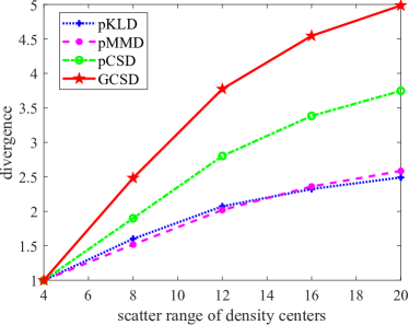
(a) With varying scatter range.

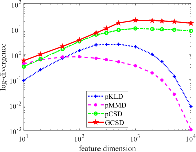
(b) With varying dimension.

Figure 3: Comparison of divergence measures. (a) The evaluation is conducted on univariate random data samples from 10 distributions. To ensure a fair comparison, measurements of all the metrics are normalized by dividing them by their respective minimum values. (b) The evaluation is conducted on multivariate samples from 3 distributions (${\cal{N}}_{1},{\cal{N}}_{2}$, and ${\cal{U}}_{1}$ as illustrated in 3.4.1 and Figure 7) with their dimension varying from $10^{1}$ to $10^{4}$. To provide a clear visual representation, we use logarithmic scaling for all measured values.

3.4.3 High-dimensional Robustness Test

To further evaluate the performances of GCSD in high-dimensional space, we conduct experiments on multivariate data across varying dimensions. The feature dimensions in each sub-distribution are varied from $10^{1}$ to $10^{4}$ and the results are presented in Figure 3b. As can be discovered, the proposed GCSD exhibits an ascending trend with the feature dimension and then a minor performance degradation when the feature dimension of testing samples exceeds $10^{3}$. In contrast, the pKLD and pMMD tend to struggle or even fail to measure the divergence of data with high dimensions.

4 Application for Deep Clustering

4.1 Advancing Clustering

Given a dataset $X$ with $n\;i.i.d.$ samples $\left\{\mathbf{x}_{i}\right\}_{i=1}^{n}$, the task of (hard) clustering refers to dividing the $n$ samples into $m$ distinct clusters $C_{1},C_{2},\cdots,C_{m}$, such that

$$\begin{split}\left\{C_{t}\right\}_{t=1}^{m}=\arg\mathop{\max}\limits_{{C_{t}}\subset X}{\rm{Dis}}\left({{C_{1}},\cdots,{C_{m}}}\right)\quad s.t.\quad\bigcup\nolimits_{t=1}^{m}{{C_{t}}}=X.\end{split}$$ (21)

where “Dis” refers to a dissimilarity measure.

A lingering question, however, is how to partition the entire observation set $X$ into $m$ groups. A practical approach is to learn the cluster assignments, represented as a soft assignment matrix $A=\left[a_{i,j}\right]\in\mathbb{R}^{n\times m}$, directly from the data using a network. Each row in $A$ corresponds to a soft pseudo-label $y_{i}$=$\left[{{a_{i,1}},{a_{i,2}},\cdots,{a_{i,m}}}\right]$, and satisfies $\sum\nolimits_{t=1}^{m}{{a_{i,t}}}=1$, where $a_{i,t}$ represents the crisp cluster assignment of data sample $i$ belonging to cluster $C_{t}$. The proposed GCSD measure can then be extended for clustering by leveraging the assignment matrix $A$.

Proposition 1

Given dataset $X=\left\{\mathbf{x}_{i}\right\}_{i=1}^{n}$ with $\mathbf{x}_{i}\in\mathbb{R}^{d}$ and its cluster-assignment matrix $A\in\mathbb{R}^{n\times m}$, the generalized Cauchy-Schwarz divergence amongst the clusters that have been partitioned from $X$ with the assignment matrix $A$ can be computed as:

$${\hat{D}}_{\rm{GCS}}^{A}({\cal P}_{1:m})= -\log\left({\frac{1}{m}{\rm{sum}}\left({\frac{{{{\left({A^{T}}\right)}^{m-1}}}}{{KA}}{\rm{prod}}\left({KA}\right)}\right)}\right)$$ (22)

$$+\frac{1}{m}{\rm{tr}}\left({\log\left({{{\left({{A^{T}}}\right)}^{m-1}}{{\left({KA}\right)}^{m-1}}}\right)}\right),$$

where $K$ represents the Gram matrix obtained by evaluating the positive definite kernel ${\kappa_{\sigma}}$ on all sample pairs, such that $K_{i,j}={\kappa_{\sigma}}({\bf x}_{i}-{\bf x}_{j})$. The notation ${\rm{sum}}(\cdot)$ signifies the summation of all elements within a matrix, ${\rm{prod}}(A)$ calculates the product of row elements in matrix $A$, yielding a column vector. For instance, ${\rm{prod}}(A)=\left[{\prod\nolimits_{j=1}^{m}{{a_{1,j}}},\cdots,\prod\nolimits_{j=1}^{m}{{a_{n,j}}}}\right]^{T}$. Furthermore, ${\rm{tr}}(\cdot)$ denotes the trace of the provided matrix. Additionally, the symbols $A^{n}$, and $\frac{A}{B}$ represent element-wise exponentiation, and division for matrices, respectively.

4.2 Deep Divergence-based Clustering Framework

The deep embedded clustering (DEC) method [4] significantly improves clustering performance on high-dimensional complex data by employing neural networks to extract features and optimizing a KLD-based clustering objective with a self-training target distribution. Subsequently, research on deep learning-based clustering methods has experienced a substantial surge [36, 37, 38]. In recent years, Jenssen et al. adeptly integrated deep learning with divergence maximization to introduce a novel clustering framework, termed deep divergence-based clustering (DDC) [5, 15, 39], effectively harnessing the potential of divergence measures for clustering applications. It should be noted that Jenssen et al. utilized the pCSD in their DDC methods, which is not a generalized divergence measure.

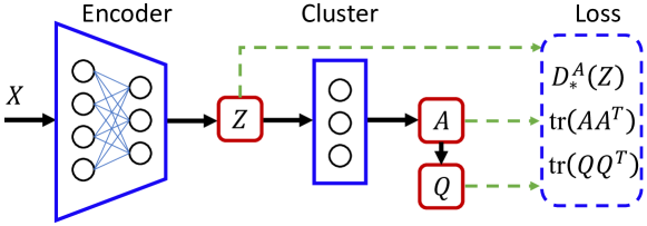
Figure 4: Deep divergence-based clustering framework. The Encoder can be implemented using various neural network architectures, such as a simple multilayer perceptron (MLP) for flattened data, a convolutional neural network (CNN) for image-like two-dimensional data, or recurrent neural networks (RNNs) like GRU or LSTM for sequential data. The Cluster can be implemented using a fully connected layer followed by softmax activation, allowing for the creation of a cluster assignment matrix. The loss function $\rm{Loss}$ integrates a generalized divergence measure $D_{*}^{A}(\cdot)$ and two regularization terms on assignment matrix $A$ to preserve its simplex property.

Figure 4 provides a conceptual overview of the deep divergence-based clustering framework. First, the input samples $\{X_{i}\}_{i=1}^{n}$ to be clustered are mapped to latent representations $\{Z_{i}\}_{i=1}^{n}$ using a deep neural network, denoted as the Encoder. Subsequently, these latent representations are passed through the Cluster network, which consists of a fully connected output layer with a softmax activation function. This process produces the (soft) cluster membership vectors $\{{\mathbf{\alpha}}_{i}\}_{i=1}^{n}$ and consequently constructs the assignment matrix $A$.

Ultimately, the framework can be trained end-to-end by maximizing the generalized divergence among the latent groups virtually clustered by the assignment matrix $A$:

$$\theta=\arg\mathop{\max}\limits_{\theta\in{\Theta}}{{\hat{D}}_{*}^{A}}\left({Z}\right).$$ (23)

Here, ${\hat{D}}_{*}^{A}$ refers to either the GCSD in Eq. (22) or another kind of generalized divergence measure.

To optimally cluster the data, the assignment matrix $A$ requires appropriate regularization. Following [5], we add two terms to the objective function in Eq. (23) to form the total loss function:

$$L={D_{*}^{A}}\left({Z}\right)+{\lambda_{2}}{\rm{tr}}\left({{AA^{T}}}\right)+{\lambda_{3}}{\rm{tr}}\left({Q{Q^{T}}}\right),$$ (24)

where ${\lambda_{2}}>0,{\lambda_{3}}>0$ are the weights used for regularization.

The second term in the loss function is calculated as the trace of the matrix $AA^{T}$, which promotes orthogonality among the clusters in the $m$-dimensional observation space. The third term enforces the proximity of the cluster membership vectors to a corner of the simplex. In this paper, $Q\in\mathbb{R}^{n\times m}$ has the same dimension as $A$ and its $(i,j)$-th entry is formulated as:

$${Q_{i,j}}=\exp\left({-{{\left|{{{\boldsymbol{\alpha}}_{i}}-{{\mathbf{e}}_{j}}}\right|}^{2}}}\right),$$ (25)

where ${\boldsymbol{\alpha}}_{i}$ is the $i$-th row of matrix $A$ and ${\mathbf{e}}_{j}\in\mathbb{R}^{m}$ is a unit vector representing the $j$-th corner of the simplex. By employing this regularizer, we ensure that the model generates a simplex assignment matrix $A$.

4.3 Clustering Experiment

We evaluate the proposed divergence measure through clustering experiments conducted on several image and time-series datasets. The comparison methods include three classical baselines: K-means [40], spectral clustering (SC) [41], and DEC [4], the SOTA deep divergence-based clustering approach (DDC) [5] and two recent proposed deep clustering methods EDESC [42] and VMM [43]. Please notice that the DDC employs the average-pairwise CSD in the loss function [5]. All models are trained for 100 epochs using a learning rate of $1e^{-3}$ and a batch size of 100. The weights of the regularization term in the loss function are set to $\lambda_{2}=\lambda_{3}=0.5$.

4.3.1 Evaluate metrics

We use two different metrics to evaluate the partition quality of the trained model. The first metric is the unsupervised clustering accuracy, ${{\rm{ACC}}=\mathop{\max}\limits_{\cal M}\sum\nolimits_{i}{{{\delta\left({{l_{i}}={\cal M}\left({{c_{i}}}\right)}\right)}\mathord{\left/{\vphantom{{\delta\left({{l_{i}}=M\left({{c_{i}}}\right)}\right)}n}}\right.\kern-1.2pt}n}}}$, where $l_{i}$ refers to the ground truth label, $c_{i}$ to the assigned cluster of data point $i$, and $\delta(\cdot)$ is the indicator function. $\cal M$ is the mapping function that corresponds to the optimal one-to-one assignment of clusters to label classes. The second evaluation measure is the normalized mutual information (NMI), ${{\rm{NMI}}={{2I\left({l,c}\right)}\mathord{\left/{\vphantom{{2I\left({l,c}\right)}{\left({H\left(l\right)+H\left(c\right)}\right)}}}\right.\kern-1.2pt}{\left({H\left(l\right)+H\left(c\right)}\right)}}}$, where $I(\cdot,\cdot)$ and $H(\cdot)$ denote mutual information and entropy functions, respectively.

4.3.2 Experiments On Image Data

Clustering experiments are conducted on three image datasets: MNIST [44], Fashion [45], and STL10 [46], utilizing deep clustering framework illustrated in Figure 4. In particular, for MNIST and Fashion datasets, we employ a two-layer convolutional extractor as the encoder with nodes $32$, $64$, and convolution filter sizes of $5\times 5$. Each layer is followed by a 2$\times$2 max pooling and a ReLU activation. For the cluster component, we implement a fully connected (FC) layer with 100 nodes, followed by another ReLU activation and a Softmax layer with a suitable dimensionality for the desired number of clusters. Batch normalization is applied to the FC layer for enhanced stability. For the STL10 dataset, we follow [42] to render the Resnet50 to extract the 2048 features. Results for DDC [5] and EDESC [42] on STL10 are also based on features extracted with Resnet50.

The findings presented in Table 1 clearly indicate that our method exhibits exceptional performance in terms of ACC and NMI. To be more specific, the proposed GCSD method outperforms other methods on FashionMNIST and STL10 datasets and achieves performance near to the state-of-the-art on MNIST dataset.

Table 1: Clustering results on image datasets.

Methods	MNIST		Fashion		STL10
	ACC	NMI	ACC	NMI	ACC	NMI
Kmeans ([40], 1979)	0.53	0.50	0.51	0.51	0.22	0.14
SC ([41], 2000)	0.69	0.77	0.56	0.57	0.17	0.11
DEC ([4], 2016)	0.77	0.72	0.58	0.62	0.17	0.05
DDC ([5], 2019)	0.85	0.79	0.68	0.61	0.84	0.80
EDESC ([42], 2022)	0.91	0.86	0.63	0.67	0.74	0.69
VMM ([43], 2024)	0.96	0.90	0.71	0.65	–	–
GCSD	0.95	0.89	0.72	0.65	0.92	0.85

• It is worth noting that DDC [5] uses the average-pairwise CSD as the divergence measure.

In addition to quantitative analysis, we provide a visualization of a mini-batch from the MNIST dataset as in Figure 5, showing the clustering results obtained by the GCSD and DDC methods. It reveals that the models trained with DDC and GJRD both often struggle to distinguish between pairs $\left\{{{\rm{1,8}}}\right\}$, $\left\{{{\rm{2,7}}}\right\}$, $\left\{{{\rm{2,8}}}\right\}$, $\left\{{\rm{5,8}}\right\}$, and $\left\{{{\rm{6,8}}}\right\}$, guiding them to mimic human observers, who often face similar challenges when distinguishing specific pairs of handwritten digits.

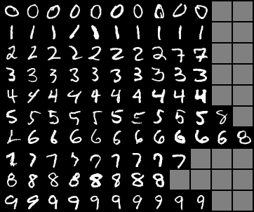
(a) GCSD

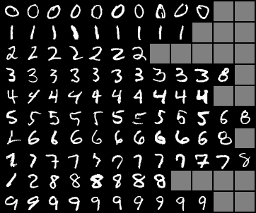
(b) DDC

Figure 5: Visualization of the clustered examples. A mini-batch of 100 samples clustered into 10 groups, each of which presented in a line. Groups with fewer clustered samples are filled with random noises.

4.3.3 Experiments On Time Series

We conducted a comparative evaluation using three benchmark time-series datasets from the UCI Machine Learning Repository [47] and a challenging video dataset derived from a portion of the Dynamic Texture dataset [48]. These four datasets, namely Arabic Digits (AD), Basic Motions (BM), ECG200 (ECG), and Animal Running (AR).

In the current experiment, the encoder is implemented using a recurrent network followed by a fully connected layer for the AD, BM, and ECG datasets. Specifically, we employ a two-layer, 32-unit bidirectional Gated Recurrent Unit (GRU) [49] to embed each time series into a vector. To handle video data from the AR dataset, a two-layer 3D CNN with 200 nodes in each layer and convolution filter sizes of $3\times 3\times 3$ is utilized before the GRU constructs the encoder.

Clustering results, as detailed in Table 2, demonstrate that the proposed GCSD method outperforms other methods on nearly all the datasets.

Table 2: Clustering Results of Time-series Datasets

Methods	AD		BM		ECG		AR
	ACC	NMI	ACC	NMI	ACC	NMI	ACC	NMI
Kmeans ([40], 1979)	0.28	0.32	0.48	0.31	0.73	0.12	0.24	0.27
SC ([41], 2000)	-	0.61	-	0.76	-	0.23	-	-
DEC ([4], 2016)	-	0.67	-	0.38	-	0.16	-	-
DDC ([5], 2019)	0.80	0.77	0.91	0.79	0.74	0.26	0.77	0.80
GCSD	0.81	0.75	0.93	0.85	0.79	0.39	0.80	0.83

• Short underlines “-” in the table indicate that no results for such dataset or metric are presented in the referenced paper.

5 Application for Domain Adaptation

5.1 Advancing Multi-Source Domain Adaptation

Assume we have a collection of $s$ source domains and one target domain $\left\{{\mathcal{D}}_{1}^{S},{\mathcal{D}}_{2}^{S},\cdots,{\mathcal{D}}_{s}^{S},{\cal{D}}^{T}\right\},$ each of which follows a specific distribution ${\mathcal{P}}_{t}$ defined on the space ${\mathcal{X}}\times{\mathcal{Y}}$. Suppose we can get access to labeled features for source domain ${\mathcal{D}}_{t}^{S}$ with a sample set of $n_{t}$ $i.i.d.$ samples $(X_{t}^{S},Y_{t}^{S})=\{\mathbf{x}_{t,i}^{S},\mathbf{y}_{t,i}^{S}\}_{i=1}^{n_{t}}$, but unlabeled features for the target domain with a sample set $X^{T}=\{\mathbf{x}_{i}^{T}\}_{i=1}^{n_{T}}$. The goal of multi-source domain adaptation (MSDA) is to learn a model $f:\mathcal{X}\rightarrow\mathcal{Y}$ with the given data that achieves optimal classification performance on the target domain.

Pioneers in the field of MSDA have made significant advancements by harnessing the power of deep learning. Their methodologies entail minimizing a loss function that quantifies the discrepancy between the target domain and each source domain [50, 51]. This process facilitates the learning of domain-invariant representations that are universally applicable across all domains. Zhu et al. developed the Multiple Feature Spaces Adaption Network (MFSAN) [19] with domain-specific feature extractors and classifiers besides the shared feature extractor for all domains. Peng et al. [7] propose the M³SDA to address the MSDA task by dynamically matching not only the moments of feature distributions between each pair of the source and target domains but also the pairs of source domains. They tried to train the feature extractor by minimizing the average-pairwise MMD or negative log-likelihood between the feature distributions of different domains and achieved superior performance to existing methods.

Building upon the concept of M³SDA [7], the training objective function for a deep learning model in the context of MSDA, incorporating moment matching or aligning of marginal distribution as an objective, can be expressed as follows:

$$\begin{array}[]{c}J=\mathop{\min}\limits_{G,C}\;\sum\nolimits_{i=1}^{s}{{\rm{CE}}\left({C\left({G\left({X_{i}^{S}}\right)}\right),Y_{i}^{S}}\right)}\\ +\lambda\sum\nolimits_{i=1}^{s}{{\rm{Dis}}\left({G\left({X_{i}^{S}}\right),G\left({{X^{T}}}\right)}\right)}+\gamma\sum\nolimits_{i<j}^{S}{{\rm{Dis}}\left({G\left({X_{i}^{S}}\right),G\left({X_{j}^{S}}\right)}\right)}.\end{array}$$ (26)

Here, “$\rm{CE}$” represents the cross entropy to obtain good classification performance for each source domain, “$\rm{Dis}$” is some kind of distance or divergence measure to implement distribution aligning or their moment matching between different domain pairs. $G$ and $C$ denote the feature extractor and classifier, respectively.

The weights $\lambda$ and $\gamma$ are used to balance the corresponding regularization terms, and different settings for them can help us achieve different goals. For instance, if we choose $\gamma=0$, the objective function will prioritize aligning the source domains with the target domain, while disregarding the alignment among the source domains themselves. Now let’s show how to implement the above objective with our proposed GCSD measure.

If taking $\lambda=\gamma$, then we can calculate the last two parts in Eq. (26) simultaneously with

$$\begin{array}[]{c}\lambda(\sum\nolimits_{i=1}^{s}{{\rm{Dis}}\left({G\left({X_{i}^{S}}\right),G\left({{X^{T}}}\right)}\right)}+\sum\nolimits_{i<j}^{s}{{\rm{Dis}}\left({G\left({X_{i}^{S}}\right),G\left({X_{j}^{S}}\right)}\right)})=:\\ \lambda{\hat{D}_{{\rm{GCS}}}}\left({G\left({X_{1}^{S}}\right),\cdots,G\left({X_{s}^{S}}\right),G\left({X^{T}}\right)}\right),\end{array}$$ (27)

where $\hat{D}_{\rm{GCS}}$ can be estimated with Eq. (16).

Thus, the objective presented in Eq. (26) can be rewritten as

$$J=\mathop{\min}\limits_{G,C}\;\sum\nolimits_{i=1}^{s}{{\rm{CE}}\left({C\left({G\left({X_{i}^{S}}\right)}\right),Y_{i}^{S}}\right)}+\lambda{\hat{D}_{\rm{GCS}}}(G(X_{1}^{S}),\cdots,G(X_{s}^{S}),G\left({X^{T}}\right)).$$ (28)

And we refer to this approach as M³SDA-GCSD.

5.2 Experiment Setup

We perform an extensive evaluation of the M³SDA-GCSD on the following tasks: digit classification on the Digits-five [7] dataset, and image recognition on the Office-31 [52], and Office-Home [53].

5.2.1 Datasets

Digits-five. The digits-five dataset is a benchmark for MSDA which includes five distinct datasets: MNIST (MT), SVHN (SV), Synthetic Digits (SD), USPS (US), and MNIST-M (MM), each containing digits ranging from 0 to 9.

Office-31. The Office-31 is a classical domain adaptation benchmark with 31 categories and 4652 images. It contains three domains: Amazon (A), Webcam (W), and DSLR (D), and the data are collected from the office environment.

Office-Home. The Office-Home dataset is composed of approximately 15,500 images distributed among 65 categories across four domains: Art (Ar), Clipart (Cl), Product (Pr), and Real World (Rw). Ar contains 2,427 paintings or artistic images from webcam sites, Cl includes 4,365 images from clipart websites, Pr consists of 4,439 webcrawled images, and Rw comprises 4,357 real-world pictures.

5.2.2 Baselines and Implementation Details

Baselines. There is a substantial amount of MSDA work on real-world visual recognition benchmarks. In our experiment, we introduce the MDAN [54], M³SDA [7], MFSAN [19], LtC-MSDA [55], and a recent deep MSDA method CASR [56] as baselines. Among them, the MDAN, M³SDA, and MFSAN are marginal distribution matching or aligning methods.

Implementation Details. We followed the setup and training procedure of the M³SDA method for the network architecture and trained them with the proposed objective presented in Eq. (28). The model framework is illustrated in Figure 6.

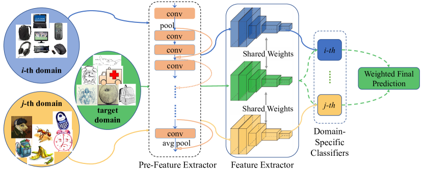
Figure 6: Multi-source domain adaptation framework. The Pre-Feature Extractor is implemented with ResNet50 or ResNet101. The Feature Extractor is implemented with CNNs and the Classifiers are Fully Connection Layers.

Specifically, for the Office-31 and the Office-Home dataset, we utilize ResNet-50 and ResNet-101 [57], respectively, as a feature extractor without any trainable parameters. Features of the image data are extracted through the ResNet and then fed into a shared extractor $G$, which consists of a three-layer conventional network with hidden nodes $512-256-128$, convolution filter size 3, stride 2, and padding 1. Each conventional layer is followed by batch-normalization and ReLU activation and a $3\times 3$ max pooling layer.

For the Digits-Five dataset, we use no pre-feature extractor but only a three-layer conventional ($conv$) followed by two fully connected linear ($fc$) for the shared feature extractor $G$, whose architecture is consistent with the M³SDA.

All the experiments are conducted with a learning rate $2.0e^{-4}$, maximum epochs 100, batch size 128 for Digits-Five, and 64 for other datasets. During training, the regularization weight $\lambda$ for $D_{*}$ is set to 0.5 for all the experiments.

5.3 Results and Comparison

The classification results on three benchmark datasets are shown in Table 3, 4, and 5. As can be seen, M³SDA-GCSD achieves superior performance in most of the transfer tasks. In terms of average accuracy, it outperforms all the compared baseline methods by significant margins, particularly in classification tasks involving more classes.

It is worth noting that the M³SDA-GCSD improves the average classification accuracy quite a lot from the original M³SDA. Specifically, the improvement approaches 7.6% for the Digits-five dataset, 11.1% for the Office-31 dataset, and 11.3% for Office-Home. Additionally, it is found that our method significantly reduces the performance deviation across different transfer tasks. This implies that the proposed method outperforms competing approaches in achieving better generalization across different domains.

The observed improvements in both average accuracy and its deviation demonstrate that minimizing the generalized divergence measure effectively aligns the feature distributions of the given domains, resulting in significant domain adaptation and generalization capability. This finding suggests that there is significant potential to employ generalized divergence measures like the proposed GCSD to align feature distributions from different domains.

Table 3: Classification accuracy (%) on Digits-five dataset.

Methods	$\to$MM	$\to$MT	$\to$US	$\to$SV	$\to$SD	AVG
MDAN ([54], 2018)	69.5	98	92.4	69.2	87.4	83.3$\pm$13.3
M3SDA ([7], 2019)	72.8	98.4	96.1	81.3	89.6	87.7$\pm$10.6
LtC-MSDA ([55], 2020)	85.6	99	98.3	83.2	93	91.8$\pm$7.2
CASR ([56], 2023)	90.2	99.7	98.3	86.4	96.3	94.1$\pm$5.7
M3SDA-GCSD	95.6	99.0	99.3	85.0	97.5	95.3$\pm$5.9

• “$\to$ * ” denotes a transfer task from domains without * to *. Our M³SDA-GCSD achieves 95.3% average accuracy, outperforming other baselines by a large margin.

Table 4: Classification accuracy (%) on Office-31 dataset.

Methods	$\to$A	$\to$W	$\to$D	AVG
MDAN ([54], 2018)	55.2	95.4	99.2	83.3$\pm$24.4
M3SDA ([7], 2019)	55.4	96.2	99.4	83.7$\pm$24.5
MFSAN ([19], 2019)	72.5	98.5	99.5	90.2$\pm$20.2
LtC-MSDA ([55], 2020)	63.9	98.4	99.2	87.2$\pm$24.0
CASR ([56], 2023)	76.2	99.8	99.8	91.9$\pm$13.6
M3SDA-GCSD	84.6	100	99.6	94.8$\pm$8.8

Table 5: Classification accuracy (%) on Office-Home dataset.

Methods	$\to$A	$\to$C	$\to$P	$\to$R	AVG
MDAN ([54], 2018)	64.9	49.7	69.2	76.3	65.0$\pm$11.2
M3SDA ([7], 2019)	64.1	62.8	76.2	78.6	70.4$\pm$8.1
MFSAN ([19], 2019)	72.1	62	80.3	81.8	74.1$\pm$9.1
CASR ([56], 2023)	72.2	61.1	82.8	82.8	74.7$\pm$10.4
M3SDA-GCSD	78.3	74.2	89.5	84.7	81.7$\pm$6.7

6 Conclusion

This paper proposes a novel generalized divergence measure named the generalized Cauchy-Schwarz divergence for multiple distributions. We provide a closed-form empirical estimator using kernel density estimation for the proposed divergence, making it suitable and convenient for machine-learning applications. Through complexity analysis and power testing, we demonstrate that our proposed GCSD can efficiently and effectively quantify dissimilarities among multiple distributions, regardless of whether they are in low or high-dimensional spaces. To further evaluate the performance of GCSD, we apply it to two challenging machine-learning tasks: deep clustering and multi-source domain adaptation. The experimental results from various benchmark datasets offer strong evidence for the exceptional power of GCSD in measuring the overall divergence of multiple distributions. The proposed method consistently outperforms existing methods in both clustering and domain adaptation across nearly all investigated datasets. The remarkable performance of GCSD in both applications highlights its substantial value in practical machine learning, thereby highlighting the potential of utilizing generalized divergence measures in machine learning domains that involve the quantification of multiple distributions.

Appendix A Details for Power Test Experiment

We generated datasets from synthetic multiple distributions to evaluate the effectiveness of our proposed divergence measures and three pairwise versions of competitors, namely pairwise Kullback–Leibler Divergence (pKLD), pairwise Maximum Mean Divergence (pMMD), and pairwise Cauchy-Schwarz Divergence (pCSD). The pairwise divergence measure is defined as the average of pairwise divergences between each two of all the $m$ distributions.

$${D_{*}}\left({\left\{{{P_{i}}}\right\}_{1}^{m}}\right)=\sum\limits_{i,j}^{m}{{d_{*}}\left({{P_{i}},{P_{j}}}\right)},$$ (29)

where $d_{*}$ can be referred to KLD, MMD, and CSD. It is important to note that the MMD is a two-sample divergence estimator. In contrast, both the KLD and the CSD are defined on continuous space for distributions. Therefore, we implement both of them with KDE.

The synthetic dataset includes ten distributions with different density centers, the range of which is scaled by a given value $r$. The ten distributions consisted of three Gaussians, three Uniforms, two bimodal Gaussians, and two bimodal Uniforms, with the corresponding probability density functions as follows:

$$\begin{array}[]{l}\begin{array}[]{*{20}{l}}{{f_{1}}\left(x\right)={\cal N}\left({0,1}\right)}&{{f_{2}}\left(x\right)={\cal N}\left({s,1}\right)}&{{f_{3}}\left(x\right)={\cal N}\left({-s,1}\right)}\\ {{f_{4}}\left(x\right)={\cal U}\left({-s,s}\right)}&{{f_{5}}\left(x\right)={\cal U}\left({-3s,-2s}\right)}&{{f_{6}}\left(x\right)={\cal U}\left({2s,3s}\right)}\end{array}\\ \begin{array}[]{*{20}{l}}{{f_{7}}\left(x\right)=0.3{\cal N}\left({-5s,1}\right)+0.7{\cal N}\left({3s,1}\right)}&{{f_{8}}\left(x\right)=0.3{\cal N}\left({-3s,1}\right)+0.7{\cal N}\left({5s,1}\right)}\\ {{f_{9}}\left(x\right)=0.3{\cal U}\left({-4s,-3s}\right)+0.7{\cal U}\left({s,2s}\right)}&{{f_{10}}\left(x\right)=0.3{\cal U}\left({3s,4s}\right)+0.7{\cal U}\left({-2s,-s}\right)}\end{array}\end{array}.$$ (30)

Here, $s=\frac{r}{10}$, and ${\cal N}(\mu,\sigma)$ represents the probability density function of a normal distribution with mean $\mu$ and standard deviation $\sigma$. Similarly, $U(l,u)$ denotes the Uniform distribution with $l$ and $u$ as the lower and upper bounds, respectively. Visualization of the synthetic data with scatter range $r=20$ (The distance from the leftmost density center to the rightmost density center) is shown in Figure 7.

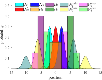
Figure 7: Test data visualization

Intuitively, the parameter $r$ controls the scattering range of the multi-distribution, which means that the sample sets from such synthetic distribution combinations with a larger $r$ value are more dispersed, thus resulting in a larger divergence. To test the effectiveness of our proposed divergence measures, we generated five sample sets using the multi-distribution defined above with scaling ranges of $r\in\left\{4,8,12,16,20\right\}$. Each distribution contributed 2000 samples, making the total size of the test dataset to be size 20000. We then conducted divergence tests on these five sample sets using the proposed GCSD and the three competing pairwise divergences mentioned earlier. Figure 8a shows the divergence measured by various metrics and Figure 8b depicts the time consumption by them.

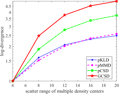
(a) Normalized divergence

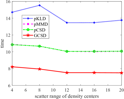
(b) Time consumption

Figure 8: Divergences measured and time consumption.

Appendix B Deduction of Proposition 1

Continuing with the deduction presented in Eq. (14)$\sim$(15), we derive

$${\hat{V}}_{1} ={\frac{1}{m}\sum\nolimits_{t=1}^{m}{\frac{1}{{{n_{t}}}}\sum\nolimits_{j=1}^{{n_{t}}}{\left({\prod\nolimits_{k\neq t}^{m}{\frac{1}{{{n_{k}}}}\sum\nolimits_{i=1}^{{n_{k}}}{{\kappa_{\sigma}}\left({{\rm{x}}_{j}^{t}-{\rm{x}}_{i}^{k}}\right)}}}\right)}}}$$ (31)

$$={\frac{1}{m}\sum\nolimits_{t=1}^{m}{\frac{1}{n}\sum\nolimits_{j=1}^{n}{\left({\prod\nolimits_{k\neq t}^{m}{{a_{j,t}}\frac{1}{n}\sum\nolimits_{i=1}^{n}{{a_{i,k}}{\kappa_{\sigma}}\left({{{\rm{x}}_{j}}-{{\rm{x}}_{i}}}\right)}}}\right)}}}$$

$$={\frac{1}{{m{n^{m}}}}\sum\nolimits_{t=1}^{m}{\sum\nolimits_{j=1}^{n}{\left({a_{j,t}^{m-1}{\rm{prod}}\left({{K_{j}}A}\right)/{K_{j}}{\alpha_{t}}}\right)}}}$$

$$={\frac{1}{{m{n^{m}}}}{\rm{sum}}\left({\frac{{{{\left({{A^{m-1}}}\right)}^{T}}}}{{KA}}{\rm{prod}}\left({KA}\right)}\right)},$$

and

$$\frac{1}{m}\sum\nolimits_{t=1}^{m}{\log\left({\hat{V}}_{2}\right)} =\frac{1}{m}\sum\nolimits_{t=1}^{m}{\log\left({\frac{1}{{{n_{t}}}}\sum\nolimits_{j=1}^{{n_{t}}}{p_{t}^{m-1}\left({{{\rm{x}}_{j}}}\right)}}\right)}$$ (32)

$$=\frac{1}{m}\sum\nolimits_{t=1}^{m}{\log\left({\frac{1}{{{n_{t}}}}\sum\nolimits_{j=1}^{{n_{t}}}{{{\left({\frac{1}{{{n_{t}}}}\sum\nolimits_{i=1}^{{n_{t}}}{{\kappa_{\sigma}}\left({{\rm{x}}_{j}^{t}-{\rm{x}}_{i}^{t}}\right)}}\right)}^{m-1}}}}\right)}$$

$$=\frac{1}{m}\sum\nolimits_{t=1}^{m}{\log\left({\frac{1}{{{n^{m}}}}\sum\nolimits_{j=1}^{n}{{{\left({\sum\nolimits_{i=1}^{n}{{a_{i,t}}{a_{j,t}}{\kappa_{\sigma}}\left({{{\rm{x}}_{j}}-{{\rm{x}}_{i}}}\right)}}\right)}^{m-1}}}}\right)}$$

$$=\frac{1}{m}\sum\nolimits_{t=1}^{m}{\log\left({\frac{1}{{{n^{m}}}}\sum\nolimits_{j=1}^{n}{{{\left({{a_{j,t}}{K_{j}}{\alpha_{t}}}\right)}^{m-1}}}}\right)}$$

$$=\frac{1}{m}{\rm{tr}}\left({\log\left({\frac{1}{{{n^{m}}}}{{\left({{A^{T}}}\right)}^{m-1}}{{\left({KA}\right)}^{m-1}}}\right)}\right).$$

Here and after, $K$ represents the Gram matrix obtained by evaluating the positive definite kernel ${\kappa_{\sigma}}$ on all sample pairs, such that $K_{i,j}={\kappa_{\sigma}}({\bf x}_{i}-{\bf x}_{j})$. The notation ${\rm{sum}}(\cdot)$ signifies the summation of all elements within a matrix. The function ${\rm{prod}}(A)$ calculates the product of row elements in matrix $A$, yielding a column vector, specifically, ${\rm{prod}}(A)=\left[{\prod\nolimits_{j=1}^{m}{{A_{1,j}}},\cdots,\prod\nolimits_{j=1}^{m}{{A_{n,j}}}}\right]^{T}$. Furthermore, ${\rm{tr}}(\cdot)$ denotes the trace of the provided matrix. Additionally, the symbols $A^{n}$, and $\frac{A}{B}$ represent element-wise exponentiation, and division for matrices, respectively.

Take Eq. (31) $\sim$ (32) into Eq. (3), we obtain the Proposition 1 as below.

Proposition 2

Given data samples $\left\{\mathbf{x}_{i}\right\}_{i=1}^{n}\in\mathbb{R}^{d}$ as well as their cluster-assignment matrix $A\in\mathbb{R}^{n\times m}$, the generalized Cauchy-Schwarz divergence of the dataset based on the assignment matrix can be computed as:

$${\hat{D}}_{\rm{GCS}}^{A}({\cal P}_{1:m})= -\log\left({\frac{1}{m}{\rm{sum}}\left({\frac{{{{\left({{A^{m-1}}}\right)}^{T}}}}{{KA}}{\rm{prod}}\left({KA}\right)}\right)}\right)$$ (33)

$$+\frac{1}{m}{\rm{tr}}\left({\log\left({{{\left({{A^{T}}}\right)}^{m-1}}{{\left({KA}\right)}^{m-1}}}\right)}\right).$$

References

- [1] A. Basu, H. Shioya, C. Park, Statistical Inference: The Minimum Distance Approach, 2011. doi:10.1201/b10956.
- [2] C. Zhu, F. Xiao, Z. Cao, A generalized Rényi divergence for multi-source information fusion with its application in EEG data analysis, Information Sciences 605 (2022) 225–243. doi:https://doi.org/10.1016/j.ins.2022.05.012.
- [3] Y. Huang, F. Xiao, Higher order belief divergence with its application in pattern classification, Information Sciences 635 (2023) 1–24. doi:https://doi.org/10.1016/j.ins.2023.03.095.
- [4] J. Xie, R. Girshick, A. Farhadi, Unsupervised deep embedding for clustering analysis, in: Int. Conf. Mach. Learn., PMLR, 2016, pp. 478–487.
- [5] M. Kampffmeyer, S. Løkse, F. M. Bianchi, L. Livi, A.-B. Salberg, R. Jenssen, Deep divergence-based approach to clustering, Neural Networks 113 (2019) 91–101.
- [6] Y. Wang, D. Chang, Z. Fu, Y. Zhao, Learning a bi-directional discriminative representation for deep clustering, Pattern Recognit. 137 (2023) 109237.
- [7] X. Peng, Q. Bai, X. Xia, Z. Huang, K. Saenko, B. Wang, Moment matching for multi-source domain adaptation, in: Proc. IEEE/CVF Int. Conf. Comput. Vis., 2019, pp. 1406–1415.
- [8] S. Hu, K. Zhang, Z. Chen, L. Chan, Domain generalization via multidomain discriminant analysis, in: Uncertain. Artif. Intell., PMLR, 2020, pp. 292–302.
- [9] S. Chen, L. Wang, Z. Hong, X. Yang, Domain generalization by joint-product distribution alignment, Pattern Recognit. 134 (2023) 109086.
- [10] D. P. Kingma, M. Welling, Auto-encoding variational bayes, arXiv Prepr. arXiv1312.6114 (2013).
- [11] I. Goodfellow, J. Pouget-Abadie, M. Mirza, B. Xu, D. Warde-Farley, S. Ozair, A. Courville, Y. Bengio, Generative adversarial nets, Adv. Neural Inf. Process. Syst. 27 (2014).
- [12] W. Zhuang, Y. Wen, S. Zhang, Divergence-aware federated self-supervised learning, in: Int. Conf. Learn. Represent., PMLR, 2022, pp. 1–19.
- [13] L. Pardo, Statistical inference based on divergence measures, CRC press, 2018.
- [14] G. Casella, R. L. Berger, Statistical Inference, Cengage Learning, 2021.
- [15] D. J. Trosten, S. Lokse, R. Jenssen, M. Kampffmeyer, Reconsidering representation alignment for multi-view clustering, in: Proc. IEEE/CVF Conf. Comput. Vis. pattern Recognit., 2021, pp. 1255–1265.
- [16] P. Zhou, L. Du, H. Wang, L. Shi, Y.-D. Shen, Learning a robust consensus matrix for clustering ensemble via Kullback-Leibler divergence minimization, in: Twenty-Fourth Int. Jt. Conf. Artif. Intell., 2015, pp. 4112–4118.
- [17] A. Banerjee, I. Dhillon, J. Ghosh, S. Merugu, An information theoretic analysis of maximum likelihood mixture estimation for exponential families, in: Proc. twenty-first Int. Conf. Mach. Learn., 2004, p. 8.
- [18] A. Banerjee, S. Merugu, I. S. Dhillon, J. Ghosh, J. Lafferty, Clustering with Bregman divergences., J. Mach. Learn. Res. 6 (10) (2005).
- [19] Y. Zhu, F. Zhuang, D. Wang, Aligning domain-specific distribution and classifier for cross-domain classification from multiple sources, in: Proc. AAAI Conf. Artif. Intell., Vol. 33, 2019, pp. 5989–5996.
- [20] S. Zhao, M. Gong, T. Liu, H. Fu, D. Tao, Domain generalization via entropy regularization, Adv. Neural Inf. Process. Syst. 33 (2020) 16096–16107.
- [21] R. Sibson, Information radius, Zeitschrift für Wahrscheinlichkeitstheorie und verwandte Gebiete 14 (2) (1969) 149–160.
- [22] A. Perez, “Barycenter” of a set of probability measures and its application in statistical decision, in: Compstat 1984 Proc. Comput. Stat., Springer, 1984, pp. 154–159.
- [23] L. Györfi, T. Nemetz, f-Dissimilarity. A generalization of the affinity of several distributions, Ann. Inst. Stat. Math 30 (Part A) (1978) 105–113.
- [24] M. Basseville, Information: entropies, divergences et moyennes, HAL CCSD (1996).
- [25] S. Kullback, R. A. Leibler, On information and sufficiency, Ann. Math. Stat. 22 (1) (1951) 79–86.
- [26] A. Rényi, On measures of entropy and information, in: Proc. Fourth Berkeley Symp. Math. Stat. Probab. Vol. 1 Contrib. to Theory Stat., Vol. 4, University of California Press, 1961, pp. 547–562.
- [27] J. Lin, Divergence measures based on the Shannon entropy, IEEE Trans. Inf. theory 37 (1) (1991) 145–151.
- [28] A. Ben Hamza, H. Krim, Jensen-renyi divergence measure: theoretical and computational perspectives, in: IEEE Int. Symp. Inf. Theory, 2003. Proceedings., 2003, p. 257. doi:10.1109/ISIT.2003.1228271.
- [29] J. Kapur, Matusita’s generalized measure of affinity, İstanbul University Science Faculty the Journal of Mathematics Physics and Astronomy 47 (1983) 73–80.
- [30] J. C. Principe, D. Xu, J. Fisher, S. Haykin, Information Theoretic Learning, Unsupervised Adapt. Filter. 1 (2000) 265–319.
- [31] H. Finner, A generalization of Holder’s inequality and some probability inequalities, Ann. Probab. (1992) 1893–1901.
- [32] F. Nielsen, K. Sun, S. Marchand-Maillet, On Hölder projective divergences, Entropy 19 (3) (2017) 122.
- [33] E. Parzen, On estimation of a probability density function and mode, Ann. Math. Stat. 33 (3) (1962) 1065–1076.
- [34] S. Yu, X. Yu, S. Løkse, R. Jenssen, J. C. Principe, Cauchy-schwarz divergence information bottleneck for regression, in: The Twelfth International Conference on Learning Representations, 2023.
- [35] L. Wasserman, All of nonparametric statistics, Springer Science & Business Media, 2006.
- [36] X. Guo, L. Gao, X. Liu, J. Yin, Improved deep embedded clustering with local structure preservation., in: Ijcai, Vol. 17, 2017, pp. 1753–1759.
- [37] J. Enguehard, P. O’Halloran, A. Gholipour, Semi-supervised learning with deep embedded clustering for image classification and segmentation, IEEE Access 7 (2019) 11093–11104.
- [38] Y. Ren, K. Hu, X. Dai, L. Pan, S. C. H. Hoi, Z. Xu, Semi-supervised deep embedded clustering, Neurocomputing 325 (2019) 121–130.
- [39] D. J. Trosten, A. S. Strauman, M. Kampffmeyer, R. Jenssen, Recurrent deep divergence-based clustering for simultaneous feature learning and clustering of variable length time series, in: ICASSP 2019-2019 IEEE Int. Conf. Acoust. Speech Signal Process., IEEE, 2019, pp. 3257–3261.
- [40] J. A. Hartigan, M. A. Wong, Algorithm AS 136: A k-means clustering algorithm, J. R. Stat. Soc. Ser. c (applied Stat. 28 (1) (1979) 100–108.
- [41] J. Shi, J. Malik, Normalized cuts and image segmentation, IEEE Trans. Pattern Anal. Mach. Intell. 22 (8) (2000) 888–905.
- [42] J. Cai, J. Fan, W. Guo, S. Wang, Y. Zhang, Z. Zhang, Efficient deep embedded subspace clustering, in: Proc. IEEE/CVF Conf. Comput. Vis. Pattern Recognit., 2022, pp. 1–10.
- [43] A. Stirn, D. A. Knowles, The VampPrior Mixture Model (2024). arXiv:2402.04412.
- [44] Y. LeCun, L. Bottou, Y. Bengio, P. Haffner, Gradient-based learning applied to document recognition, Proc. IEEE 86 (11) (1998) 2278–2324.
- [45] H. Xiao, K. Rasul, R. Vollgraf, Fashion-mnist: a novel image dataset for benchmarking machine learning algorithms, arXiv Prepr. arXiv1708.07747 (2017).
- [46] A. Coates, A. Ng, H. Lee, An analysis of single-layer networks in unsupervised feature learning, in: Proc. fourteenth Int. Conf. Artif. Intell. Stat., JMLR Workshop and Conference Proceedings, 2011, pp. 215–223.
- [47] A. Asuncion, D. Newman, UCI machine learning repository (2007).
- [48] R. Péteri, S. Fazekas, M. J. Huiskes, DynTex: A comprehensive database of dynamic textures, Pattern Recognit. Lett. 31 (12) (2010) 1627–1632.
- [49] K. Cho, B. Van Merriënboer, C. Gulcehre, D. Bahdanau, F. Bougares, H. Schwenk, Y. Bengio, Learning phrase representations using RNN encoder-decoder for statistical machine translation, arXiv Prepr. arXiv1406.1078 (2014).
- [50] R. Xu, Z. Chen, W. Zuo, J. Yan, L. Lin, Deep cocktail network: Multi-source unsupervised domain adaptation with category shift, in: Proc. IEEE Conf. Comput. Vis. pattern Recognit., 2018, pp. 3964–3973.
- [51] H. Zhao, S. Zhang, G. Wu, J. P. Costeira, J. M. F. Moura, G. J. Gordon, Multiple source domain adaptation with adversarial learning, in: Work. Track Sixth Int. Conf. Learn. Represent., 2018, pp. 1–24.
- [52] K. Saenko, B. Kulis, M. Fritz, T. Darrell, Adapting visual category models to new domains, in: Comput. Vision–ECCV 2010 11th Eur. Conf. Comput. Vision, Heraklion, Crete, Greece, Sept. 5-11, 2010, Proceedings, Part IV 11, Springer, 2010, pp. 213–226.
- [53] H. Venkateswara, J. Eusebio, S. Chakraborty, S. Panchanathan, Deep hashing network for unsupervised domain adaptation, in: Proc. IEEE Conf. Comput. Vis. pattern Recognit., 2017, pp. 5018–5027.
- [54] H. Zhao, S. Zhang, G. Wu, J. M. F. Moura, J. P. Costeira, G. J. Gordon, Adversarial multiple source domain adaptation, Adv. Neural Inf. Process. Syst. 31 (2018).
- [55] H. Wang, M. Xu, B. Ni, W. Zhang, Learning to combine: Knowledge aggregation for multi-source domain adaptation, in: Comput. Vision–ECCV 2020 16th Eur. Conf. Glas. UK, August 23–28, 2020, Proceedings, Part VIII 16, Springer, 2020, pp. 727–744.
- [56] S. Wang, B. Wang, Z. Zhang, A. A. Heidari, H. Chen, Class-aware sample reweighting optimal transport for multi-source domain adaptation, Neurocomputing 523 (2023) 213–223.
- [57] K. He, X. Zhang, S. Ren, J. Sun, Deep residual learning for image recognition, in: Proc. IEEE Conf. Comput. Vis. pattern Recognit., 2016, pp. 770–778.