Joint Visibility Region Detection and Channel Estimation for XL-MIMO Systems via
Alternating MAP

Abstract

We investigate a joint visibility region (VR) detection and channel estimation problem in extremely large-scale multiple-input-multiple-output (XL-MIMO) systems, where near-field propagation and spatial non-stationary effects exist. In this case, each scatterer can only see a subset of antennas, i.e., it has a certain VR over the antennas. Because of the spatial correlation among adjacent sub-arrays, VR of scatterers exhibits a two-dimensional (2D) clustered sparsity. We design a 2D Markov prior model to capture such a structured sparsity. Based on this, a novel alternating maximum a posteriori (MAP) framework is developed for high-accuracy VR detection and channel estimation. The alternating MAP framework consists of three basic modules: a channel estimation module, a VR detection module, and a grid update module. Specifically, the first module is a low-complexity inverse-free variational Bayesian inference (IF-VBI) algorithm that avoids the matrix inverse via minimizing a relaxed Kullback-Leibler (KL) divergence. The second module is a structured expectation propagation (EP) algorithm which has the ability to deal with complicated prior information. And the third module refines polar-domain grid parameters via gradient ascent. Simulations demonstrate the superiority of the proposed algorithm in both VR detection and channel estimation.

I Introduction

High-frequency extremely large-scale multiple-input-multiple-output (XL-MIMO) has been widely considered as a key technology for future 6G communications [1]. With the deployment of hundreds or even thousands of antennas, XL-MIMO systems can mitigate many of the challenges faced in traditional massive MIMO systems [2], offering unprecedented data rates and enhancing the overall performance of wireless networks. Meanwhile, for extremely high-frequency communications, such as millimeter-wave (mmWave) and terahertz (THz) communications, the size of high-frequency antennas is small due to the small wavelength [3]. Therefore, it is natural to integrate XL-MIMO and high-frequency communication into 6G wireless systems [1].

However, the use of XL-MIMO and high-frequency bands will lead to some new issues compared to traditional massive MIMO systems. Above all, near-field propagation is likely to exist. Given the large antenna aperture of XL-MIMO and high-frequency, the array will exhibit a large near-field region [4]. When users or scatterers are inside the Rayleigh region, the array will experience a spherical wave, which accounts for both angle and distance parameters. Besides, spatial non-stationary is another issue in high-frequency XL-MIMO systems. Spatial non-stationary means that different regions of an extremely large-scale array can see different scatterers [5], making it quite difficult for high-accuracy channel estimation with low pilot overhead. Fortunately, the measurement in [6] verified that sub-channels corresponding to each small-scale sub-array can be treated as spatial stationary, i.e., each antenna in the same sub-array can see the same scatterers. In this case, we can focus on the visibility region (VR) detection for each sub-array instead of each antenna. Furthermore, there is spatial correlation among adjacent sub-arrays. As illustrated in Fig. 1, adjacent sub-arrays may be visible to the same scatterer with a high probability [7, 8]. In other words, the VR of a scatterer will concentrate on a few clusters and the associated VR vector/matrix will exhibit a clustered sparsity. The above characteristics of XL-MIMO channels should be fully exploited to enhance the channel estimation performance, especially in the low signal-to-noise ratio (SNR) regions. Some early attempts at XL-MIMO channel estimation and visibility region detection are summarized below.

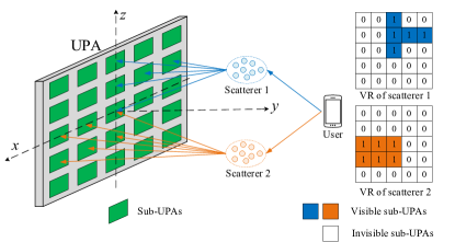
Figure 1: Illustration of spatial non-stationary and VRs in XL-MIMO systems. The VR of scatterers exhibits a clustered sparsity.

Near-field XL-MIMO channel estimation: In the case of far-field, the massive MIMO channel exhibits sparsity in the angular domain. Many algorithms based on compressive sensing (CS) have been studied to achieve sparse channel estimation [9, 10, 11]. However, in the case of near-field, the steering vector is related to both the angle and distance parameters of last-hop scatterers. As a result, the sparse representation for near-field channels is quite different. In [12], the authors proposed a polar-domain sparse representation that combined the angle and distance information simultaneously for near-field channels. Based on the polar-domain codebook, an off-grid orthogonal matching pursuit (OMP) algorithm was designed for XL-MIMO channel estimation. In [13], the authors studied a joint dictionary learning and channel estimation algorithm to reduce the complexity of the polar-domain dictionary and enhance the channel estimation performance. The authors in [14] further extended the polar-domain representation from narrow-band ULA systems to broadband uniform planar array (UPA) systems. In [15], the authors considered a sub-array hybrid precoding architecture and designed a damped Newtonized OMP algorithm for user localization and channel estimation.

Joint VR detection and channel estimation: The above research only considers the near-field effect, while the spatial non-stationary issue is not addressed. In [16, 17], the VR of scatterers and sub-arrays was studied, and the VR detection was achieved by sub-array grouping. Inspired by this, several sub-array-wise methods were studied for addressing the spatial non-stationary issue [17, 18, 19]. Specifically, the authors in [17] designed a joint VR identification, user localization, and channel estimation scheme with the aid of reconfigurable intelligent surface (RIS). An expectation-maximization (EM)-based bilinear Bayesian inference algorithm were proposed in [18] for joint VR detection and channel estimation. In [19], the authors exploited the time-domain relevance of non-stationary effect to improve the performance. Generally speaking, these sub-array-wise methods first estimate each sub-channel independently, and then combine the estimated sub-channels into the whole channel. Such approaches work poorly when the SNR is low and there are few pilots. The reasons are twofold: firstly, they ignore the fact that sub-channels share some common scatterers and the associated complex channel gain, angle, and distance information; secondly, they do not exploit the structure of VRs. To exploit these, the authors in [7, 8] used a Markov chain model to describe the clustered sparsity of VR vectors in XL-MIMO ULA systems. Based on the Markov chain model, a turbo orthogonal approximate message passing (Turbo-OAMP) algorithm was proposed. By fully exploiting the sparse structure of VR vectors, the performance of both VR detection and channel estimation was significantly improved. However, the work in [8] only considers a line-of-sight (LoS)-only channel model, and the proposed method cannot be extended to multipath channels intuitively. Moreover, when the sensing matrix is not partially orthogonal, the Turbo-OAMP algorithm will involve a high-dimensional matrix inverse each iteration, which leads to unacceptable computational overhead.

In this paper, we consider a joint VR detection and channel estimation problem in a XL-MIMO UPA system at the mmWave band. There are three main challenges in our considered problem: 1) In the scenario of UPA, the VR of scatterers will exhibit a 2D clustered sparsity, and thus a new sparse prior model is needed to capture the 2D clustered sparsity; 2) Since sub-channels corresponding to sub-arrays are correlated via shared scatterers, the whole channel and the associated channel parameters should be estimated jointly; 3) Because of the extremely large number of XL-MIMO, low-complexity algorithm design becomes essential. To overcome these challenges, we first formulate the considered problem as a bilinear observation model. Then, we introduce a two-dimensional (2D) Markov prior model to describe the 2D clustered sparsity of VRs. Finally, we design an alternating maximum a posteriori (MAP) framework with acceptable complexity for high-accuracy VR detection and channel estimation. The main contributions are summarized below.

• Prior design for VRs and the sparse channel: To exploit the 2D clustered sparsity of VRs, we design a 2D Markov prior model, which can be treated as an extension of the one-dimensional Markov chain model in [7, 8]. Moreover, we introduce a hierarchical sparse prior model to capture the sparsity of the XL-MIMO channel vector in the polar domain.

• Alternating MAP framework: We propose an alternating MAP framework that contains three basic modules: a channel estimation module, a VR detection module, and a grid update module. The three modules work alternatively to improve each other’s performance. Some approaches are employed to reduce the complexity of the alternating MAP. Firstly, inspired by [20, 21], we develop an inverse-free variational Bayesian inference (IF-VBI) algorithm as the channel estimation module, where the high-dimensional matrix inverse operation is avoided via minimizing a relaxed Kullback-Leibler (KL) divergence. Secondly, in the VR detection module, we use polar-domain filtering and sub-array grouping methods to achieve matrix dimension reduction. As such, the alternating MAP framework is able to perform high-performance VR detection and channel estimation with acceptable computational overhead.

• Structured expectation propagation (EP) algorithm: In the VR detection module, we propose a novel structured EP algorithm based on the 2D Markov prior. The structured EP algorithm consists of two modules: a linear minimum-mean-square-error (LMMSE) estimator and a non-linear MMSE estimator. Compared to the conventional EP [22], the proposed structured EP can process more complicated prior information by using loopy belief propagation in the MMSE estimator.

The paper proceeds as follows. In Section II, we show the system model. In Section III, we focus on the structured prior design for VRs and the polar-domain sparse channel vector. In Section IV, we present the novel alternating MAP framework and detail its three basic modules. Simulations and conclusions are shown in Section V and VI, respectively.

Notations: Lowercase and uppercase bold letterers denote vectors and matrices, respectively. Let $\left(\cdot\right)^{-1}$, $\left(\cdot\right)^{T}$, $\left(\cdot\right)^{H}$, $\left\langle\cdot\right\rangle$, $\left\|\cdot\right\|$, $\textrm{vec}\left(\cdot\right)$, and $\textrm{diag}\left(\cdot\right)$ represent the inverse, transpose, conjugate transpose, expectation, $\ell_{2}\textrm{-norm}$, vectorization, and diagonalization operations, respectively. $\otimes$ is the Kronecker product operator and $\odot$ means the Hadamard product operator. $\Re\left\{\cdot\right\}$ and $\Im\left\{\cdot\right\}$ denote the real and imaginary part of the complex argument, respectively. $\mathbf{I}_{N}$ is the $N\times N$ dimensional identity matrix and $\mathbf{1}_{M\times N}$ is the $M\times N$ dimensional all-one matrix. For a set $\mathbf{\Omega}$ with its cardinal number denoted by $\left|\mathbf{\Omega}\right|$, $\boldsymbol{x}\triangleq\left[x_{n}\right]_{n\in\mathbf{\Omega}}\in\mathbb{C}^{\left|\mathbf{\Omega}\right|\times 1}$ is a vector composed of elements indexed by $\mathbf{\Omega}$. $\mathcal{CN}\left(\boldsymbol{x};\boldsymbol{\mu},\mathbf{\Sigma}\right)$ denotes the complex Gaussian distribution with mean $\boldsymbol{\mu}$ and covariance $\mathbf{\Sigma}$. $\textrm{Ga}\left(x;a,b\right)$ denotes the Gamma distribution with shape parameter $a$ and rate parameter $b$.

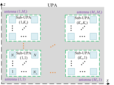
Figure 2: The structure of the UPA and the index rule of antennas and sub-UPAs.

II System Model

II-A Introduction of the XL-MIMO System

Consider a XL-MIMO system operating at the mmWave band, where one base station (BS) serves a single-antenna user, as shown in Fig. 1. The BS is equipped with a half-wavelength UPA of $M=M_{x}\times M_{z}$ antennas in the $x\textrm{-}z$ plane. The large-scale UPA is partitioned into $K=K_{x}\times K_{z}$ small-scale sub-UPAs, with each sub-UPA consisting of $N=N_{x}\times N_{z}$ antennas, where $N_{x}=\frac{M_{x}}{K_{x}}$ and $N_{z}=\frac{M_{z}}{K_{z}}$, as illustrated in Fig. 2. The carrier frequency is $f$ and the wavelength is $\lambda_{c}=\frac{c}{f}$, where $c$ is the speed of light. The spacing between two adjacent antennas is $d=\frac{\lambda_{c}}{2}$, and the antenna aperture is given by $D=\sqrt{\left(M_{x}-1\right)^{2}+\left(M_{z}-1\right)^{2}}d$. For convenience, we set the center of the UPA as the origin $\left[0,0,0\right]^{T}$ of the coordinate system. Index the antenna in the bottom left corner as the $\left(1,1\right)\textrm{-th}$ antenna, as presented in Fig. 2. Define the relative subscript of the $\left(m_{x},m_{z}\right)\textrm{-th}$ antenna as $\left(\delta_{m_{x}},\delta_{m_{z}}\right)=\left(m_{x}-\frac{M_{x}+1}{2},m_{z}-\frac{M_{z}+1}{2}\right)$, then the coordinates of the $\left(m_{x},m_{z}\right)\textrm{-th}$ antenna can be expressed as $\boldsymbol{p}_{m_{x},m_{z}}=\left[\delta_{m_{x}}d,0,\delta_{m_{z}}d\right]^{T}$. The user transmits an uplink pilot symbol (assume the pilot is equal to one without loss of generality), then the received signal at the BS can be expressed as

$$\boldsymbol{y}=\boldsymbol{h}+\boldsymbol{w},$$ (1)

where $\boldsymbol{h}\in\mathbb{C}^{M\times 1}$ is the channel vector and $\boldsymbol{w}\sim\mathcal{CN}\left(0,1/\gamma\mathbf{I}_{M}\right)$ is the additive white Gaussian noise (AWGN) with variance $1/\gamma$. As near-field propagation and spatial non-stationary effects exist, the structure of the channel vector is quite different from that of far-field massive MIMO channels and will be exploited to significantly improve the channel estimation performance.

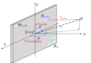
Figure 3: The distance, azimuth angle, and elevation angle of a scatterer in the coordinate system.

II-B Near-field Spatial Non-stationary Channel Model

In XL-MIMO systems at the mmWave band, the Rayleigh distance is hundreds of meters [4], and thus near-field propagation cannot be neglected. The impact of near-field propagation is primarily reflected in the steering vector. Let $\theta$, $\varphi$, and $r$ denote the azimuth angle, elevation angle, and distance of a scatterer with respect to the origin, respectively, as illustrated in Fig. 3. The coordinates of the scatterer can be expressed as $\boldsymbol{p}=\left[r\cos\theta\sin\varphi,r\sin\theta\sin\varphi,r\cos\varphi\right]^{T}$. Then the distance between the scatterer and the $\left(m_{x},m_{z}\right)\textrm{-th}$ antenna of the UPA is given by

$$r_{m_{x},m_{z}}=\left\|\boldsymbol{p}-\boldsymbol{p}_{m_{x},m_{z}}\right\|=$$ (2)

$$\sqrt{r^{2}+\delta_{m_{x}}^{2}d^{2}+\delta_{m_{z}}^{2}d^{2}-2r\delta_{m_{x}}d\cos\theta\sin\varphi-2r\delta_{m_{z}}d\cos\varphi}.$$

Referring to the uniform spherical wave (USW) model [23, 4], the steering vector is derived as

$$\boldsymbol{a}\left(\theta,\varphi,r\right)= \frac{1}{\sqrt{M}}\left[e^{-j\frac{2\pi}{\lambda_{c}}\left(r_{1,1}-r\right)},\ldots,e^{-j\frac{2\pi}{\lambda_{c}}\left(r_{M_{x},1}-r\right)},\ldots,\right.$$

$$\left.e^{-j\frac{2\pi}{\lambda_{c}}\left(r_{1,M_{z}}-r\right)},\ldots,e^{-j\frac{2\pi}{\lambda_{c}}\left(r_{M_{x},M_{z}}-r\right)}\right]^{T}.$$ (3)

The Fresnel approximation is usually introduced to simplify the complicated expressions in (2) and (3). Based on the Fresnel approximation [24], the distance $r_{m_{x},m_{z}}$ is approximate to

$$r_{m_{x},m_{z}}\approx r-\delta_{m_{x}}d\cos\theta\sin\varphi+\frac{\delta_{m_{x}}^{2}d^{2}\left(1-\cos^{2}\theta\sin^{2}\varphi\right)}{2r}$$

$$-\delta_{m_{z}}d\cos\varphi+\frac{\delta_{m_{z}}^{2}d^{2}\left(1-\cos^{2}\varphi\right)}{2r}.$$ (4)

Let $\vartheta\triangleq\cos\theta\sin\varphi$ and $\phi\triangleq\cos\varphi$, the steering vector under the Fresnel approximation can be obtained as

$$\boldsymbol{a}\left(\vartheta,\phi,r\right)=\frac{1}{\sqrt{M}}\boldsymbol{a}_{z}\left(\phi,r\right)\otimes\boldsymbol{a}_{x}\left(\vartheta,r\right),$$ (5)

with

$$\left[\boldsymbol{a}_{x}\left(\vartheta,r\right)\right]_{m_{x}} =e^{-j\frac{2\pi}{\lambda_{c}}\left(-\delta_{m_{x}}d\vartheta+\frac{\delta_{m_{x}}^{2}d^{2}\left(1-\vartheta^{2}\right)}{2r}\right)},$$ (6a)

$$\left[\boldsymbol{a}_{z}\left(\phi,r\right)\right]_{m_{z}} =e^{-j\frac{2\pi}{\lambda_{c}}\left(-\delta_{m_{z}}d\phi+\frac{\delta_{m_{z}}^{2}d^{2}\left(1-\phi^{2}\right)}{2r}\right)},$$ (6b)

where $\left[\boldsymbol{a}_{x}\left(\vartheta,r\right)\right]_{m_{x}}$ is the $m_{x}\textrm{-th}$ element of $\boldsymbol{a}_{x}\left(\vartheta,r\right)$ for $m_{x}=1,\ldots,M_{x}$, and $\left[\boldsymbol{a}_{z}\left(\phi,r\right)\right]_{m_{z}}$ is the $m_{z}\textrm{-th}$ element of $\boldsymbol{a}_{z}\left(\phi,r\right)$ for $m_{z}=1,\ldots,M_{z}$. The work in [24] has verified that the Fresnel approximation is accurate enough when the distance between the scatterer and the BS is large than the Fresnel distance. Note that the Fresnel distance $0.5\sqrt{\frac{D^{3}}{\lambda_{c}}}$ is much smaller than the Rayleigh distance $\frac{2D^{2}}{\lambda_{c}}$. For instance, if the antenna aperture is $D=1\ \textrm{m}$ and the carrier frequency is $f=30\ \textrm{GHz}$, then the Rayleigh distance will be $200\ \textrm{m}$, while the Fresnel distance will be only $5\ \textrm{m}$ that can nearly be neglected.

Besides, the spatial non-stationary effect is also obvious in XL-MIMO systems [5], i.e., different regions of the UPA will receive different levels of power due to different scatterers they can see. Assume there are $L$ paths between the user and the BS, and we only focus on the last-hop scatterer of the paths. We define a binary matrix

$$\mathbf{V}_{l}=\left[\begin{array}[]{cccc}v_{l,1,1}&v_{l,1,2}&\cdots&v_{l,1,K_{z}}\\ v_{l,2,1}&v_{l,2,2}&\cdots&v_{l,2,K_{z}}\\ \vdots&\vdots&\ddots&\vdots\\ v_{l,K_{x},1}&v_{l,K_{x},2}&\cdots&v_{l,K_{x},K_{z}}\end{array}\right],$$ (7)

to represent the visibility region of scatterer $l$ for $l=1,\ldots,L$, where $v_{l,k_{x},k_{z}}=1$ indicates scatterer $l$ can see sub-UPA $\left(k_{x},k_{z}\right)$ and $v_{l,k_{x},k_{z}}=0$ indicates the opposite.

Based on these, the channel vector $\boldsymbol{h}$ can be modeled as

$$\boldsymbol{h}=\sum_{l=1}^{L}x_{l}\boldsymbol{a}\left(\vartheta_{l},\phi_{l},r_{l}\right)\odot\boldsymbol{u}_{l},$$ (8)

where $x_{l}$ denotes the complex gain of the $l\textrm{-th}$ path and $r_{l}$ is the distance of scatterer $l$. $\vartheta_{l}\triangleq\cos\theta_{l}\sin\varphi_{l}$ and $\phi_{l}\triangleq\cos\varphi_{l}$, in which $\theta_{l}$ and $\varphi_{l}$ are the azimuth and elevation angles of scatterer $l$, respectively. $\boldsymbol{a}\left(\vartheta_{l},\phi_{l},r_{l}\right)$ is the steering vector simulated by scatterer $l$ and $\boldsymbol{u}_{l}\triangleq\textrm{vec}\left(\mathbf{V}_{l}\otimes\mathbf{1}_{N_{x}\times N_{z}}\right)$ is the element-level VR vector.

Moreover, there is spatial correlation among adjacent sub-UPAs, i.e., adjacent sub-UPAs may be visible to the same scatterer with a high probability. In this case, the binary matrix $\mathbf{V}_{l},\forall l$ exhibits a 2D clustered sparsity. Therefore, it is essential to design a sparse prior model to capture such a structured sparsity.

III Prior Design for VRs and the Polar-domain Channel

In this section, we first introduce a polar-domain sparse representation method for the XL-MIMO channel. Then, we present sparse probability models for both VRs and the sparse channel vector. Finally, the joint VR detection and channel estimation problem is formulated as a MAP estimation problem.

III-A Polar-domain Sparse Representation Method

We adopt the grid-based method to obtain a sparse representation of the XL-MIMO channel for high-accuracy channel estimation. In [12, 14], the authors verified that the near-field channel exhibits sparsity in the polar domain, which accounts for both angle and distance information simultaneously. Inspired by this, we design a 3-D polar-domain grid for the case of UPA. Specifically, we first introduce a angle gird of $M_{1}\times M_{2}$ angle points, in which the sampling points $\left\{\bar{\vartheta}_{m_{1}}\right\}_{m_{1}=1}^{M_{1}}$ and $\left\{\bar{\phi}_{m_{2}}\right\}_{m_{2=1}}^{M_{2}}$ are uniformly distributed within $[-1,1]$. Then, at the sampled angle $\left(\bar{\vartheta}_{m_{1}},\bar{\phi}_{m_{2}}\right),\forall m_{1},m_{2}$, the distance sampling points $\left\{\bar{r}_{m_{1},m_{2},n}\right\}_{n=1}^{N_{m_{1},m_{2}}}$ can be obtained using Algorithm 1 in [12], where $N_{m_{1},m_{2}}$ denotes the number of sampled distances at direction $\left(\bar{\vartheta}_{m_{1}},\bar{\phi}_{m_{2}}\right)$. Based on these, the polar-domain grid points can be expressed as

$$\bar{\boldsymbol{\Xi}}\triangleq \Bigl{[}\bigl{[}\bar{\vartheta}_{1},\bar{\phi}_{1},\bar{r}_{1}\bigr{]};\ldots;\bigl{[}\bar{\vartheta}_{1},\bar{\phi}_{1},\bar{r}_{N_{1,1}}\bigr{]};\ldots$$ (9)

$$\bigl{[}\bar{\vartheta}_{m_{1}},\bar{\phi}_{m_{2}},\bar{r}_{1}\bigr{]};\ldots;\bigl{[}\bar{\vartheta}_{m_{1}},\bar{\phi}_{m_{2}},\bar{r}_{N_{m_{1},m_{2}}}\bigr{]};\ldots$$

$$\bigl{[}\bar{\vartheta}_{M_{1}},\bar{\phi}_{M_{2}},\bar{r}_{1}\bigr{]};\ldots;\bigl{[}\bar{\vartheta}_{M_{1}},\bar{\phi}_{M_{2}},\bar{r}_{N_{M_{1},M_{2}}}\bigr{]}\Bigr{]}.$$

The total number of grid points is given by $Q=\sum_{m_{1}=1}^{M_{1}}\sum_{m_{2}=1}^{M_{2}}N_{m_{1},m_{2}}$. To simply the notation, we use $q$ to index the grid points in $\bar{\boldsymbol{\Xi}}$, and the $q\textrm{-th}$ polar-domain grid point (i.e., the $q\textrm{-th}$ row of $\bar{\boldsymbol{\Xi}}$) is denoted by $\left[\bar{\vartheta}_{q},\bar{\phi}_{q},\bar{r}_{q}\right]$ for $q=1,\ldots,Q$.

However, in practice, the true angle-distances of scatterers usually do not lie exactly on the discrete polar-domain grid points. As a result, there exists a mismatch between the true angle-distance and its nearest grid point, which will lead to an energy leakage effect. In the high SNR regions, the leakage effect caused by angle and distance mismatch is especially obvious, which cannot be neglected compared to the noise power. Therefore, we introduce a dynamic polar-domain grid, denoted by $\boldsymbol{\Xi}\triangleq\left[\boldsymbol{\vartheta},\boldsymbol{\phi},\boldsymbol{r}\right]$, instead of only using a fixed grid, where $\boldsymbol{\vartheta}\triangleq\left[\vartheta_{1},\ldots,\vartheta_{Q}\right]^{T}$, $\boldsymbol{\phi}\triangleq\left[\phi_{1},\ldots,\phi_{Q}\right]^{T}$, and $\boldsymbol{r}\triangleq\left[r_{1},\ldots,r_{Q}\right]^{T}$ denote angle and distance dynamic grid vectors. The fixed grid $\bar{\boldsymbol{\Xi}}$ is chosen as the initial value of $\boldsymbol{\Xi}$, and the grid parameters are updated via gradient ascent during algorithm design.

With the definition of the dynamic polar-domain grid, we can obtain a polar-domain sparse basis as

$$\left[\mathbf{A}\left(\boldsymbol{\Xi}\right)\right]_{q}=\left[\boldsymbol{a}\left(\vartheta_{q},\phi_{q},r_{q}\right)\right],\forall q,$$ (10)

where $\left[\mathbf{A}\left(\boldsymbol{\Xi}\right)\right]_{q}$ denotes the $q\textrm{-th}$ column of $\mathbf{A}\left(\boldsymbol{\Xi}\right)\in\mathbb{C}^{M\times Q}$. Besides, let $\mathbf{V}_{q}\in\left\{0,1\right\}^{K_{x}\times K_{z}}$ represent the VR of the scatterer lying around the $q\textrm{-th}$ grid point and denote the collection of VRs as $\mathbf{V}\triangleq\left\{\mathbf{V}_{q}\mid\forall q\right\}$. Define $\mathbf{U}\left(\mathbf{V}\right)\triangleq\left[\boldsymbol{u}_{1},\ldots,\boldsymbol{u}_{Q}\right]\in\mathbb{C}^{M\times Q}$ as the VR dictionary corresponding to the polar-domain grid, where $\boldsymbol{u}_{q}\triangleq\textrm{vec}\left(\mathbf{V}_{q}\otimes\mathbf{1}_{N_{x}\times N_{z}}\right),\forall q$. Then the sparse representation of the channel vector in (8) can be obtained as

$$\boldsymbol{h} =\left[\mathbf{A}\left(\boldsymbol{\Xi}\right)\odot\mathbf{U}\left(\mathbf{V}\right)\right]\boldsymbol{x},$$ (11)

where $\boldsymbol{x}\in\mathbb{C}^{Q\times 1}$ is the polar-domain sparse channel vector, which has only $L\ll Q$ non-zero elements corresponding to $L$ paths. Specifically, the $q\textrm{-th}$ element of $\boldsymbol{x}$, denoted by $x_{q}$, is the complex gain of the channel path with the corresponding scatterer lying around the $q\textrm{-th}$ grid point.

Note that the transform matrix in (11), denoted by $\mathbf{A}\left(\boldsymbol{\Xi}\right)\odot\mathbf{U}\left(\mathbf{V}\right)$, is quite different from that in [12, 14] due to the existing of spatial non-stationary. The VR dictionary $\mathbf{U}\left(\mathbf{V}\right)$ provides the VR information of each scatterer lying in the polar-domain grid.

III-B Sparse Probability Model

In this subsection, we first design a 2D Markov model to capture the 2D clustered sparsity of VRs. Besides, a hierarchical sparse prior model is used to describe the sparsity of the polar-domain channel vector. Finally, we obtain the joint distribution of all variables.

III-B1 2D Markov model for VRs

Since the VR of scatterers exhibits a 2D clustered sparsity, the non-zero elements in $\mathbf{V}_{q},\forall q$ will concentrate on a few clusters. This implies that $v_{q,k_{x},k_{z}}$ depends on both $v_{q,k_{x}-1,k_{z}}$ and $v_{q,k_{x},k_{z}-1}$. Specifically, if $v_{q,k_{x},k_{z}-1}=1$ or $v_{q,k_{x},k_{z}-1}=1$, there is a higher probability that $v_{q,k_{x},k_{z}}=1$. Such a structured sparsity can be modeled using the 2D Markov model [25],

$$p\left(\mathbf{V}_{q}\right)= p\left(v_{q,1,1}\right)\prod_{k_{x}=2}^{K_{x}}\prod_{k_{z}=1}^{K_{z}}p\left(v_{q,k_{x},k_{z}}\mid v_{q,k_{x}-1,k_{z}}\right)$$

$$\times\prod_{k_{x}=1}^{K_{x}}\prod_{k_{z}=2}^{K_{z}}p\left(v_{q,k_{x},k_{z}}\mid v_{q,k_{x},k_{z}-1}\right),\forall q,$$ (12)

with the transition probability given by

$$p_{01}^{x} =p\left(v_{q,k_{x},k_{z}}=1\mid v_{q,k_{x}-1,k_{z}}=0\right),$$ (13a)

$$p_{10}^{x} =p\left(v_{q,k_{x},k_{z}}=0\mid v_{q,k_{x}-1,k_{z}}=1\right),$$ (13b)

$$p_{01}^{z} =p\left(v_{q,k_{x},k_{z}}=1\mid v_{q,k_{x},k_{z}-1}=0\right),$$ (13c)

$$p_{10}^{z} =p\left(v_{q,k_{x},k_{z}}=0\mid v_{q,k_{x},k_{z}-1}=1\right).$$ (13d)

Note that [25] has verified that a set of $\left\{p_{01}^{x},p_{10}^{x},p_{01}^{z},p_{10}^{z}\right\}$ can be found to satisfy the steady-state condition of the 2D Markov model, i.e., $p\left(v_{q,k_{x},k_{z}}=1\right)=\kappa,\forall k_{x},k_{z}$, where $\kappa$ defined as the visibility probability shows the sparsity level of $\mathbf{V}_{q}$. As such, the initial distribution $p\left(v_{q,1,1}\right)$ is set to be the steady-state distribution, $p\left(v_{q,1,1}=1\right)=\kappa$. The factor graph of the 2D Markov model is presented in Fig. 6.

The value of $\left\{p_{01}^{x},p_{10}^{x},p_{01}^{z},p_{10}^{z}\right\}$ will affect the structure of clusters. Specifically, smaller $p_{10}^{x}$ and $p_{10}^{z}$ imply a larger average cluster size, and smaller $p_{01}^{x}$ and $p_{01}^{z}$ imply a larger average gap between two adjacent clusters. Therefore, the 2D Markov model has the flexibility to characterize the 2D clustered sparsity of $\mathbf{V}_{q}$.

III-B2 Hierarchical sparse prior for the channel

We introduce a hierarchical sparse prior model to capture the sparsity of the polar-domain channel vector $\boldsymbol{x}$, as illustrated in Fig. 4. Specifically, let $\boldsymbol{s}\triangleq\left[s_{1},\ldots,s_{Q}\right]^{T}$ denote the support of $\boldsymbol{x}$, where $s_{q}=1$ indicates $x_{q}$ is non-zero and $s_{q}=0$ indicates the opposite. Let $\boldsymbol{\rho}\triangleq\left[\rho_{1},\ldots,\rho_{Q}\right]^{T}$ denote the precision vector of $\boldsymbol{x}$, where $1/\rho_{q}$ gives the variance of $x_{q}$. The variables $\boldsymbol{x}$, $\boldsymbol{\rho}$, and $\boldsymbol{s}$ form a Markov chain, denoted by $\boldsymbol{s}\rightarrow\boldsymbol{\rho}\rightarrow\boldsymbol{x}$, and the joint distribution can be expressed as

$$p\left(\boldsymbol{x},\boldsymbol{\rho},\boldsymbol{s}\right)=\underbrace{p\left(\boldsymbol{s}\right)}_{\textrm{Support}}\underbrace{p\left(\boldsymbol{\rho}\mid\boldsymbol{s}\right)}_{\textrm{Precision}}\underbrace{p\left(\boldsymbol{x}\mid\boldsymbol{\rho}\right)}_{\textrm{Sparse\ signal}}.$$ (14)

For an independent sparse structure, a Bernoulli prior is usually used to model the support vector [26, 27],

$$p\left(\boldsymbol{s}\right)=\prod_{q=1}^{Q}\left(\lambda_{q}\right)^{s_{q}}\left(1-\lambda_{q}\right)^{1-s_{q}},$$ (15)

where $\lambda_{q}$ gives the probability that $s_{q}=1$.

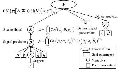
Figure 4: Illustration of the hierarchical sparse prior model.

The conditional distribution $p\left(\boldsymbol{\rho}\mid\boldsymbol{s}\right)$ is given by

$$p\left(\boldsymbol{\rho}\mid\boldsymbol{s}\right)=\prod_{q=1}^{Q}\textrm{Ga}\left(\rho_{q};a_{q},b_{q}\right)^{s_{q}}\textrm{Ga}\left(\rho_{q};\overline{a}_{q},\overline{b}_{q}\right)^{1-s_{q}}.$$ (16)

We use two different Gamma distributions to model $\rho_{q}$ according to the value of $s_{q}$. When $s_{q}=1$, the element $x_{q}$ is non-zero. In this case, the corresponding parameters of the precision $\rho_{q}$, denoted by $a_{q}$ and $b_{q}$, should be chosen to satisfy $\frac{a_{q}}{b_{q}}=\mathbb{E}\left[\rho_{q}\right]=\mathcal{O}\left(1\right)$ such that the variance of $x_{q}$ is also $\mathcal{O}\left(1\right)$. When $s_{q}=0$, the element $x_{q}$ is zero or close to zero. In this case, the corresponding parameters of the precision $\rho_{q}$, denoted by $\overline{a}_{q}$ and $\overline{b}_{q}$, should be chosen to satisfy $\frac{\overline{a}_{q}}{\overline{b}_{q}}=\mathbb{E}\left[\rho_{q}\right]\gg 1$ such that the variance of $x_{q}$ is close to zero. The motivation for choosing Gamma is that the Gamma distribution is a conjugate of the Gaussian prior, which facilitates closed-form Bayesian inference [28, 29, 30].

The conditional distribution $p\left(\boldsymbol{x}\mid\boldsymbol{\rho}\right)$ is given by

$$p\left(\boldsymbol{x}\mid\boldsymbol{\rho}\right)=\prod_{q=1}^{Q}p\left(x_{q}\mid\rho_{q}\right)=\prod_{q=1}^{Q}\mathcal{CN}\left(x_{q};0,\rho_{q}^{-1}\right).$$ (17)

In practice, the exact distribution of each element of $\boldsymbol{x}$ is usually unknown. Nevertheless, it is reasonable to choose a hierarchical Gaussian prior with Gamma-distributed precision for $\boldsymbol{x}$. Firstly, the Gaussian prior facilitates low-complexity algorithm design. Secondly, the existing VBI-type algorithms derived from such a hierarchical prior are well known to be insensitive to the true distribution of $\boldsymbol{x}$ [28, 29, 30].

Moreover, we use a Gamma distribution with parameters $c$ and $d$ to model the noise precision [28, 29, 30],

$$p\left(\gamma\right)=\textrm{Ga}\left(\gamma;c,d\right).$$ (18)

According to the existing works [31, 32, 21, 33], the hierarchical sparse prior model is robust w.r.t. the the imperfect prior information in practice, and it is tractable to enable low-complexity and high-performance algorithm design.

III-B3 The joint distribution

The joint distribution of the random variables discussed above is given by

$$p\left(\boldsymbol{y},\mathbf{V},\boldsymbol{x},\boldsymbol{\rho},\boldsymbol{s},\gamma;\boldsymbol{\Xi}\right)= p\left(\boldsymbol{y}\mid\mathbf{V},\boldsymbol{x},\gamma;\boldsymbol{\Xi}\right)$$

$$\times\prod_{q=1}^{Q}p\left(\mathbf{V}_{q}\right)p\left(\boldsymbol{x},\boldsymbol{\rho},\boldsymbol{s}\right)p\left(\gamma\right),$$ (19)

with the likelihood function given by

$$p\left(\boldsymbol{y}\mid\mathbf{V},\boldsymbol{x},\gamma;\boldsymbol{\Xi}\right)= \mathcal{CN}\left(\boldsymbol{y};\left[\mathbf{A}\left(\boldsymbol{\Xi}\right)\varodot\mathbf{U}\left(\mathbf{V}\right)\right]\boldsymbol{x},\gamma^{-1}\mathbf{I}_{M}\right).$$

III-C The MAP Problem Formulation

Using the polar-domain sparse representation in (11), the received signal in (1) can be written into an observation model with unknown VRs and uncertain grid parameters in the sensing matrix,

$$\boldsymbol{y}=\left[\mathbf{A}\left(\boldsymbol{\Xi}\right)\odot\mathbf{U}\left(\mathbf{V}\right)\right]\boldsymbol{x}+\boldsymbol{w}.$$ (20)

Since it is quite difficult to perform Bayesian inference for all variables, we aim at computing the MAP estimate of the channel vector $\boldsymbol{x}$, the VRs $\mathbf{V}$, and the grid parameters $\boldsymbol{\Xi}$ given the observation $\boldsymbol{y}$, i.e.,

$$\boldsymbol{x}^{\dagger},\mathbf{V}^{\dagger},\boldsymbol{\Xi}^{\dagger}=\underset{\boldsymbol{x},\mathbf{V},\boldsymbol{\Xi}}{\arg\max}\ln p\left(\boldsymbol{y},\mathbf{V},\boldsymbol{x},\boldsymbol{\rho},\boldsymbol{s},\gamma;\boldsymbol{\Xi}\right),$$ (21)

where the joint distribution $p\left(\boldsymbol{y},\mathbf{V},\boldsymbol{x},\boldsymbol{\rho},\boldsymbol{s},\gamma;\boldsymbol{\Xi}\right)$ is given in (19). However, it is still intractable to directly solve the MAP problem in (21) since different variables have quite different priors and likelihood functions. To address this problem, we update the MAP estimate of each variable in an alternating way. Specifically, for given $\hat{\mathbf{V}}$ and $\hat{\boldsymbol{\Xi}}$, we perform Bayesian inference to compute the marginal posterior distribution of $\boldsymbol{x}$ and $\gamma$, denoted by $q\left(\boldsymbol{x}\mid\boldsymbol{y},\hat{\mathbf{V}};\hat{\boldsymbol{\Xi}}\right)$ and $q\left(\gamma\mid\boldsymbol{y},\hat{\mathbf{V}};\hat{\boldsymbol{\Xi}}\right)$, respectively. Then the MAP estimate of $\boldsymbol{x}$ is obtained as $\hat{\boldsymbol{x}}=\textrm{arg}\max_{\boldsymbol{x}}q\left(\boldsymbol{x}\mid\boldsymbol{y},\hat{\mathbf{V}};\hat{\boldsymbol{\Xi}}\right)$ and the MMSE estimate of $\gamma$ is obtained as $\hat{\gamma}=\int\gamma q\left(\gamma\mid\boldsymbol{y},\hat{\mathbf{V}};\hat{\boldsymbol{\Xi}}\right)\textrm{d}\gamma$. For given $\hat{\boldsymbol{x}}$, $\hat{\gamma}$, and $\hat{\boldsymbol{\Xi}}$, we compute the approximate posterior distribution $p\left(\mathbf{V}_{q}\mid\boldsymbol{y},\hat{\boldsymbol{x}},\hat{\gamma};\hat{\boldsymbol{\Xi}}\right),\forall q$ using a structured EP algorithm and obtain the MAP estimate of $\mathbf{V}_{q}$ as $\mathbf{\hat{V}}_{q}=\textrm{arg}\max_{\mathbf{V}_{q}}p\left(\mathbf{V}_{q}\mid\boldsymbol{y},\hat{\boldsymbol{x}},\hat{\gamma};\hat{\boldsymbol{\Xi}}\right)$. Meanwhile, based on $\hat{\boldsymbol{x}}$, $\hat{\gamma}$, and $\hat{\mathbf{V}}$, the grid parameters are obtained by the MAP estimator as $\hat{\boldsymbol{\Xi}}=\textrm{arg}\max_{\boldsymbol{\Xi}}\ln p\left(\boldsymbol{\Xi}\mid\boldsymbol{y},\hat{\mathbf{V}},\hat{\boldsymbol{x}},\hat{\gamma}\right)$.

There are two main challenges during algorithm design for the MAP problem. Firstly, the conventional Bayesian inference algorithms (when updating $\boldsymbol{x}$ and $\gamma$) usually involve a matrix inverse each iteration, whose complexity is unacceptable when the number of XL-MIMO array is large. Secondly, the conventional EP algorithm is unable to compute the posterior distribution of $\mathbf{V}$ since the 2D Markov prior is quite complicated and the corresponding factor graph contains loops. Therefore, it is exceedingly challenging to design a high-efficient algorithm with acceptable complexity for the considered MAP problem. In the following section, we propose a novel alternating MAP framework to overcome these challenges.

IV The Alternating MAP Framework

IV-A Outline of the Alternating MAP Framework

The alternating MAP framework consists of three basic modules: the channel estimation module, the VR detection module, and the grid update module, as illustrated in Fig. 5. The three modules work alternatively until convergence. In the following, we give a brief introduction to the three modules.

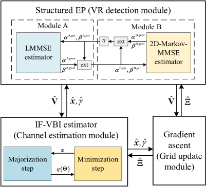
Figure 5: The alternating MAP framework and its three basic modules.

• Channel estimation module: It is a low-complexity IF-VBI estimator that avoids the matrix inverse via minimizing a relaxed KL divergence. For given $\hat{\mathbf{V}}$ and $\hat{\boldsymbol{\Xi}}$, the IF-VBI estimator optimizes the marginal posterior distribution of $\boldsymbol{x}$, $\boldsymbol{\rho}$, $\boldsymbol{s}$, and $\gamma$ alternatively. Then, the MAP estimate of $\boldsymbol{x}$ and the MMSE estimate of $\gamma$ are obtained based on the corresponding marginal posterior distribution.

• VR detection module: It is a structured EP algorithm that combines the LMMSE estimator and the 2D-Markov-MMSE estimator via a turbo approach. For given $\hat{\boldsymbol{x}}$, $\hat{\gamma}$, and $\hat{\boldsymbol{\Xi}}$, the structured EP computes the posterior distribution of $\mathbf{V}_{q},\forall q$ approximately by combining observation information and 2D Markov prior information. And $\hat{\mathbf{V}}$ is updated by maximizing the approximate posterior distribution.

• Grid update module: Based on the $\hat{\boldsymbol{x}}$, $\hat{\gamma}$, and $\hat{\mathbf{V}}$ obtained in the other two modules, compute the gradient of $\ln p\left(\boldsymbol{y}\mid\hat{\mathbf{V}},\hat{\boldsymbol{x}},\hat{\gamma},;\boldsymbol{\Xi}\right)$ w.r.t. $\boldsymbol{\Xi}$, then update $\hat{\boldsymbol{\Xi}}$ via gradient ascent method.

IV-B IF-VBI Estimator (Channel Estimation Module)

In this module, the transform matrix in (20) is fixed since $\hat{\mathbf{V}}$ and $\hat{\boldsymbol{\Xi}}$ are given. We define $\mathbf{F}\left(\hat{\mathbf{V}},\hat{\boldsymbol{\Xi}}\right)\triangleq\mathbf{A}\left(\hat{\mathbf{V}}\right)\odot\mathbf{U}\left(\hat{\boldsymbol{\Xi}}\right)$ and omit $\hat{\mathbf{V}},\hat{\boldsymbol{\Xi}}$ in $\mathbf{F}\left(\hat{\mathbf{V}},\hat{\boldsymbol{\Xi}}\right)$ for simplicity. Now the observation model in (20) can be reformulated as $\boldsymbol{y}=\mathbf{F}\boldsymbol{x}+\boldsymbol{w}$, and the corresponding channel estimation problem is a standard compressive sensing (CS) problem. Many methods have been proposed to solve such a CS problem, among which the Turbo-OAMP in [7, 8] and AMP in [34] can achieve the best trade-off between the performance and complexity. However, since the sensing matrix $\mathbf{F}$ is neither partially orthogonal nor i.i.d., both Turbo-OAMP and AMP involve a high-dimensional matrix inverse each iteration, which leads to unacceptable computational overhead for XL-MIMO. To overcome this issue, we design a low-complexity IF-VBI algorithm.

For convenience, we define $\mathbf{\Theta}\triangleq\left\{\boldsymbol{x},\boldsymbol{\rho},\boldsymbol{s},\gamma\right\}$ as the collection of hidden variables. Let $\mathbf{\Theta}^{k}$ denote an individual variable in $\mathbf{\Theta}$ and let $\boldsymbol{\mathcal{H}}\triangleq\left\{k\mid\forall\mathbf{\Theta}^{k}\in\mathbf{\Theta}\right\}$. The mead-filed VBI method uses the variational distribution $q\left(\mathbf{\Theta}\right)$ to approximate the true posterior distribution $p\left(\mathbf{\Theta}\mid\boldsymbol{y}\right)$. And $q\left(\mathbf{\Theta}\right)$ is optimized via minimizing the KL divergence between $q\left(\mathbf{\Theta}\right)$ and $p\left(\mathbf{\Theta}\mid\boldsymbol{y}\right)$ under a factorized form constraint as

$$\min_{q\left(\mathbf{\Theta}\right)}\mathrm{KL}\left(q\parallel p\right) \triangleq\int q\left(\mathbf{\Theta}\right)\ln\frac{q\left(\mathbf{\Theta}\right)}{p\left(\mathbf{\Theta}\mid\boldsymbol{y}\right)}\mathrm{d}\boldsymbol{v},$$

$$s.t.\hskip 22.76219ptq\left(\mathbf{\Theta}\right) =\prod_{k\in\boldsymbol{\mathcal{H}}}q\left(\mathbf{\Theta}^{k}\right),$$ (22)

where $q\left(\mathbf{\Theta}\right)=\prod_{k\in\boldsymbol{\mathcal{H}}}q\left(\mathbf{\Theta}^{k}\right)$ is the constraint under the mean-field assumption [35]. The KL divergence in (22) is convex w.r.t. a single variational distribution $q\left(\mathbf{\Theta}^{k}\right)$ after fixing other variational distributions $q\left(\mathbf{\Theta}^{l}\right),\forall l\neq k$ [36]. Therefore, we can find a stationary solution of (22) via optimizing each variational distribution alternatively. And the optimal $q\left(\mathbf{\Theta}^{k}\right)$ is given by [30]

$$q\bigl{(}\mathbf{\Theta}^{k}\bigr{)}=\frac{\exp\left(\left\langle\ln p\left(\mathbf{\Theta},\boldsymbol{y}\right)\right\rangle_{\Pi_{l\neq k}q\left(\mathbf{\Theta}^{l}\right)}\right)}{\int\exp\left(\left\langle\ln p\left(\mathbf{\Theta},\boldsymbol{y}\right)\right\rangle_{\Pi_{l\neq k}q\left(\mathbf{\Theta}^{l}\right)}\right)\textrm{d}\mathbf{\Theta}^{k}},$$ (23)

where $\left\langle\cdot\right\rangle_{\Pi_{l\neq k}q\left(\mathbf{\Theta}^{l}\right)}$ represents an expectation w.r.t. $q\left(\mathbf{\Theta}^{l}\right),\forall l\neq k$. Submitting the joint distribution in (19) into (23), the update of $q\left(\boldsymbol{x}\right)$ is derived as a complex Gaussian distribution with its mean and covariance given by

$$\boldsymbol{\mu} =\mathbf{\Sigma}\left\langle\gamma\right\rangle\mathbf{F}^{H}\boldsymbol{y},$$ (24)

$$\mathbf{\Sigma} =\left(\left\langle\gamma\right\rangle\mathbf{F}^{H}\mathbf{F}+\textrm{diag}\left(\left\langle\rho\right\rangle\right)\right)^{-1}.$$

Note that the computation of $\mathbf{\Sigma}$ involves a $Q\times Q$ dimensional matrix inverse, whose complexity is $\mathcal{O}\left(Q^{3}\right)$. The computational overhead caused by the matrix inverse is very high due to the deployment of thousands of antennas in XL-MIMO systems ($M$ is large and $Q>M$).

Inspired by an inverse-free Bayesian approach in [20], we develop a low-complexity IF-VBI algorithm that avoids the matrix inverse via minimizing a relaxed KL divergence. Note that the proposed IF-VBI is a variant of the Bayesian approach in [20]. The difference is that the IF-VBI is used to deal with the hierarchical sparse prior in (14) but not the Laplace prior in [20]. The main idea of the IF-VBI is to construct a relaxed KL divergence and then minimize it based on the majorization-minimization (MM) framework [37].

Specifically, a lower bound of the likelihood function can be found by resorting to Lemma 1 in [20],

$$p\left(\boldsymbol{y}\mid\boldsymbol{x},\gamma\right)= \left(\frac{\gamma}{\pi}\right)^{M}\exp\left(-\gamma\left\|\boldsymbol{y}-\mathbf{F}\boldsymbol{x}\right\|^{2}\right)$$

$$\geq \left(\frac{\gamma}{\pi}\right)^{M}\exp\left(-\gamma g\left(\boldsymbol{x},\boldsymbol{z}\right)\right)\triangleq\mathrm{G}\left(\boldsymbol{y},\boldsymbol{x},\boldsymbol{z},\gamma\right),$$ (25)

with $g\left(\boldsymbol{x},\boldsymbol{z}\right)$ given by

$$g\left(\boldsymbol{x},\boldsymbol{z}\right)\triangleq \left\|\boldsymbol{y}-\mathbf{F}\boldsymbol{z}\right\|^{2}+T\left\|\boldsymbol{x}-\boldsymbol{z}\right\|^{2}$$

$$+2\Re\left\{\left(\boldsymbol{x}-\boldsymbol{z}\right)^{H}\mathbf{F}^{H}\left(\mathbf{F}\boldsymbol{z}-\boldsymbol{y}\right)\right\},$$ (26)

where $T$ needs to satisfy $T\mathbf{I}_{Q}\succeq\mathbf{F}^{H}\mathbf{F}$. And a good choice for $T$ is $\lambda_{\textrm{max}}\left(\mathbf{F}^{H}\mathbf{F}\right)$, where $\lambda_{\textrm{max}}\left(\cdot\right)$ denotes the largest eigenvalue of the given matrix.

Submitting (25) into (22), we construct a relaxed KL divergence as

$$\widetilde{\textrm{KL}}\left(q\parallel p\right)\triangleq\int q\left(\mathbf{\Theta}\right)\ln\frac{q\left(\mathbf{\Theta}\right)p\left(\boldsymbol{y}\right)}{\mathrm{G}\left(\boldsymbol{y},\boldsymbol{x},\boldsymbol{z},\gamma\right)p\left(\mathbf{\Theta}\right)}\mathrm{d}\boldsymbol{v},$$ (27)

which is a upper bound of $\mathrm{KL}\left(q\parallel p\right)$. Based on this, we employ the MM framework to minimize the relaxed KL divergence w.r.t. $q\left(\mathbf{\Theta}^{k}\right),\forall k$ and $\boldsymbol{z}$. Specifically, in the majorization step, we update each variational distribution alternatively after fixing $\boldsymbol{z}$. In the minimization step, we minimize $\widetilde{\textrm{KL}}\left(q\parallel p\right)$ w.r.t. $\boldsymbol{z}$ given $q\left(\mathbf{\Theta}^{k}\right),\forall k$. The IF-VBI estimator iterates between the majorization step and minimization step until convergence.

IV-B1 Majorization step (update of $q\left(\mathbf{\Theta}^{k}\right),\forall k$)

Using (23), $q\left(\boldsymbol{x}\right)$ is update as

$$\ln q\left(\boldsymbol{x}\right)\propto \left\langle\ln\mathrm{G}\left(\boldsymbol{y},\boldsymbol{x},\boldsymbol{z},\gamma\right)\right\rangle_{q\left(\gamma\right)}+\left\langle\ln p\left(\boldsymbol{x}\mid\boldsymbol{\rho}\right)\right\rangle_{q\left(\boldsymbol{\rho}\right)}$$

$$\propto -\boldsymbol{x}^{H}\left(\left\langle\gamma\right\rangle T\mathbf{I}_{Q}+\textrm{diag}\left(\left\langle\boldsymbol{\rho}\right\rangle\right)\right)\boldsymbol{x}$$

$$+2\Re\left\{\boldsymbol{x}^{H}\left\langle\gamma\right\rangle\left(\mathbf{F}^{H}\left(\boldsymbol{y}-\mathbf{F}\boldsymbol{z}\right)+T\boldsymbol{z}\right)\right\}.$$ (28)

This is a complex Gaussian distribution with mean $\boldsymbol{\mu}$ and covariance $\mathbf{\Sigma}$ given by

$$\boldsymbol{\mu} =\mathbf{\Sigma}\left\langle\gamma\right\rangle\left(\mathbf{F}^{H}\left(\boldsymbol{y}-\mathbf{F}\boldsymbol{z}\right)+T\boldsymbol{z}\right),$$ (29)

$$\mathbf{\Sigma} =\left(\left\langle\gamma\right\rangle T\mathbf{I}_{Q}+\textrm{diag}\left(\left\langle\boldsymbol{\rho}\right\rangle\right)\right)^{-1}.$$

Now $\mathbf{\Sigma}$ is calculated by a diagonal matrix inverse, which is linear complexity.

The update of $q\left(\gamma\right)$ can be derived as

$$\ln q\left(\gamma\right) \propto\left\langle\ln\mathrm{G}\left(\boldsymbol{y},\boldsymbol{x},\boldsymbol{z},\gamma\right)\right\rangle_{q\left(\boldsymbol{x}\right)}+\ln p\left(\gamma\right)$$

$$\propto\left(c-1+M\right)\ln\gamma-\left(d+\left\langle g\left(x,z\right)\right\rangle\right)\gamma,$$ (30)

with $\left\langle g\left(x,z\right)\right\rangle$ given by

$$\left\langle g\left(x,z\right)\right\rangle= \left\|\boldsymbol{y}-\mathbf{F}\boldsymbol{z}\right\|^{2}+T\left\|\boldsymbol{\mu}-\boldsymbol{z}\right\|^{2}+\textrm{Tr}\left(\mathbf{\Sigma}\right)$$

$$+2\Re\left\{\left(\boldsymbol{\mu}-\boldsymbol{z}\right)^{H}\mathbf{F}^{H}\left(\mathbf{F}\boldsymbol{z}-\boldsymbol{y}\right)\right\},$$ (31)

where $\textrm{Tr}\left(\cdot\right)$ is the trace of the given matrix. Thus, we have

$$q\left(\gamma\right)=\textrm{Ga}\left(\gamma;\tilde{c},\tilde{d}\right),$$ (32)

where the parameters $\tilde{c}$ and $\tilde{d}$ are given by

$$\tilde{c} =c+M,$$ (33)

$$\tilde{d} =d+\left\langle g\left(x,z\right)\right\rangle.$$

The variational distribution of $\boldsymbol{\rho}$ and $\boldsymbol{s}$ can be derived in a similar way. Please refer to subsection IV-D in [31] for the expression of $q\left(\boldsymbol{\rho}\right)$ and $q\left(\boldsymbol{s}\right)$.

IV-B2 Minimization step (update of $\boldsymbol{z}$)

Submitting $q\left(\mathbf{\Theta}\right)$ into $\widetilde{\textrm{KL}}\left(q\bigparallel p\right)$, $\boldsymbol{z}$ can be updated as

$$\boldsymbol{z}^{\textrm{new}}=\arg\min_{\boldsymbol{z}}\left\langle-\ln\mathrm{G}\left(\boldsymbol{y},\boldsymbol{x},\boldsymbol{z},\gamma\right)\right\rangle_{q\left(\mathbf{\Theta}\right)}.$$ (34)

Calculate the gradient of the function in (34), i.e.,

$$\nabla_{\boldsymbol{z}}\left\langle-\ln\mathrm{G}\left(\boldsymbol{y},\boldsymbol{x},\boldsymbol{z},\gamma\right)\right\rangle_{q\left(\mathbf{\Theta}\right)}=\left\langle\gamma\right\rangle\left(\mathbf{F}^{H}\mathbf{F}-T\mathbf{I}_{Q}\right)\left(\boldsymbol{\mu}-\boldsymbol{z}\right).$$ (35)

The function is minimized when the gradient becomes zero, i.e.,

$$\boldsymbol{z}^{\textrm{new}}=\boldsymbol{\mu}.$$ (36)

Finally, the MAP estimate of $\boldsymbol{x}$ and the MMSE estimate of $\boldsymbol{\gamma}$ are given by

$$\hat{\boldsymbol{x}} =\boldsymbol{\mu},$$ (37)

$$\hat{\gamma} =\frac{\tilde{c}}{\tilde{d}}.$$

IV-C Structured EP (VR Detection Module)

Given $\hat{\boldsymbol{x}}$, $\hat{\gamma}$, and $\hat{\boldsymbol{\Xi}}$, the observation model in (20) is rewritten as $\boldsymbol{y}=\left[\mathbf{A}\left(\hat{\boldsymbol{\Xi}}\right)\varodot\mathbf{U}\left(\mathbf{V}\right)\right]\hat{\boldsymbol{x}}+\boldsymbol{w}.$ We employ the sub-array grouping method since a sub-array is the basic unit keeping spatial stationary. Define the index set of the antennas in sub-array $\left(k_{x},k_{z}\right)$ as $\mathbf{\Psi}_{k_{x},k_{z}}\subseteq\left\{1,\ldots,M\right\}$, with its cardinal number given by $\left|\mathbf{\Psi}_{k_{x},k_{z}}\right|=N$. Then, the received signal of sub-array $\left(k_{x},k_{z}\right)$ is expressed as

$$\boldsymbol{y}_{k_{x},k_{z}}= \left[\mathbf{A}_{k_{x},k_{z}}\left(\hat{\boldsymbol{\Xi}}\right)\varodot\left(\mathbf{1}_{N\times 1}\hat{\boldsymbol{x}}^{T}\right)\right]\boldsymbol{v}_{k_{x},k_{z}}+\boldsymbol{w}_{k_{x},k_{z}},$$ (38)

with $\boldsymbol{y}_{k_{x},k_{z}}\triangleq\left[y_{m}\right]_{m\in\mathbf{\Psi}_{k_{x},k_{z}}}$, $\boldsymbol{w}_{k_{x},k_{z}}\triangleq\left[w_{m}\right]_{m\in\mathbf{\Psi}_{k_{x},k_{z}}}$, and $\mathbf{A}_{k_{x},k_{z}}\left(\hat{\boldsymbol{\Xi}}\right)\triangleq\left[\mathbf{A}_{m}\left(\hat{\boldsymbol{\Xi}}\right)\right]_{m\in\mathbf{\Psi}_{k_{x},k_{z}}}$. $\mathbf{A}_{m}\left(\hat{\boldsymbol{\Xi}}\right)$ denotes the $m\textrm{-th}$ row of $\mathbf{A}\left(\hat{\boldsymbol{\Xi}}\right)$, and $\boldsymbol{v}_{k_{x},k_{z}}\triangleq\left[v_{1,k_{x},k_{z}},\ldots,v_{Q,k_{x},k_{z}}\right]^{T}$ is the VR of sub-array $\left(k_{x},k_{z}\right)$. Moreover, we define $\mathbf{H}_{k_{x},k_{z}}\triangleq\mathbf{A}_{k_{x},k_{z}}\left(\hat{\boldsymbol{\Xi}}\right)\odot\left(\mathbf{1}_{N\times 1}\hat{\boldsymbol{x}}^{T}\right)$ to simplify the notation.

Note that $\hat{\boldsymbol{x}}$ has only a few non-zero element, which means that many columns of $\mathbf{H}_{k_{x},k_{z}}$ are all-zero vectors. In this case, it is difficult to estimate $\boldsymbol{v}_{k_{x},k_{z}}$ from the observation $\boldsymbol{y}_{k_{x},k_{z}}$ under an ill-conditioned sensing matrix $\mathbf{H}_{k_{x},k_{z}}$. We use a polar-domain filtering method to address this problem. Specifically, we set a small threshold $\varepsilon>0$ and compare each element of $\hat{\boldsymbol{x}}$ with the threshold. Let $\mathbf{\Omega}\triangleq\left\{q\mid\forall\left\|\hat{x}_{q}\right\|^{2}>\varepsilon\right\}$ represent the index set of the elements with the energy larger than the threshold. Then, we only retain the columns indexed by $\mathbf{\Omega}$ in $\mathbf{H}_{k_{x},k_{z}}$ and delete other columns that are close to zero. In this case, the obtained sensing matrix, denoted by $\mathbf{\ddot{H}}_{k_{x},k_{z}}\in\mathbb{C}^{N\times\left|\mathbf{\Omega}\right|}$, is well-conditioned, and the received signal model in (38) is rewritten as

$$\boldsymbol{y}_{k_{x},k_{z}}=\mathbf{\ddot{H}}_{k_{x},k_{z}}\ddot{\boldsymbol{v}}_{k_{x},k_{z}}+\boldsymbol{w}_{k_{x},k_{z}},$$ (39)

where $\ddot{\boldsymbol{v}}_{k_{x},k_{z}}\triangleq\left[v_{q,k_{x},k_{z}}\right]_{q\in\mathbf{\Omega}}$. Such a polar-domain filtering method also greatly reduces the complexity of the algorithm due to $\left|\mathbf{\Omega}\right|\ll Q$. For $q\notin\mathbf{\Omega}$, $\hat{x}_{q}$ is close to zero, which indicates that there is no scatterer lying around the $q\textrm{-th}$ polar-domain grid point. Therefore, it is unnecessary to estimate $v_{q,k_{x},k_{z}}$ for $q\notin\mathbf{\Omega}$, and we can simply set them to be zero.

Since $\ddot{\boldsymbol{v}}_{k_{x},k_{z}},\forall k_{x},k_{z}$ is real-valued, we reformulate the complex-valued model in (39) into a real-valued one,

$$\tilde{\boldsymbol{y}}_{k_{x},k_{z}}=\mathbf{\tilde{H}}_{k_{x},k_{z}}\ddot{\boldsymbol{v}}_{k_{x},k_{z}}+\tilde{\boldsymbol{w}}_{k_{x},k_{z}},$$ (40)

where $\tilde{\boldsymbol{y}}_{k_{x},k_{z}}\triangleq\left[\Re\left\{\boldsymbol{y}_{k_{x},k_{z}}\right\}^{T},\Im\left\{\boldsymbol{y}_{k_{x},k_{z}}\right\}^{T}\right]^{T}$, and $\mathbf{\tilde{H}}_{k_{x},k_{z}}$ and $\tilde{\boldsymbol{w}}_{k_{x},k_{z}}$ are defined similarly. Based on the above linear observation model, we develop a structured EP algorithm to compute the approximate posterior of $\ddot{\boldsymbol{v}}_{k_{x},k_{z}},\forall k_{x},k_{z}$.

As shown in Fig. 5, the structured EP is a turbo framework that consists of two basic modules: Module A is a LMMSE estimator that combines the observation information and messages from Module B, while Module B is called the 2D-Markov-MMSE estimator, which performs the MMSE estimation based on the 2D Markov prior and messages from Module A. The two modules exchange messages and work alternatively until convergence.

IV-C1 LMMSE in Module A

In Module A, a Gaussian distribution is assumed as the prior for $\ddot{\boldsymbol{v}}_{k_{x},k_{z}}$, denoted by $\mathcal{N}\left(\ddot{\boldsymbol{v}}_{k_{x},k_{z}};\boldsymbol{\alpha}_{k_{x},k_{z}}^{\textrm{A,pri}},\textrm{diag}\left(\boldsymbol{\beta}_{k_{x},k_{z}}^{\textrm{A,pri}}\right)\right)$, where $\boldsymbol{\alpha}_{k_{x},k_{z}}^{\textrm{A,pri}}$ and $\boldsymbol{\beta}_{k_{x},k_{z}}^{\textrm{A,pri}}$ are extrinsic messages from module B. Based on the LMMSE estimator, the posterior distribution is also a Gaussian distribution with its mean and covariance given by

$$\mathbf{\Gamma}_{k_{x},k_{z}}^{\textrm{A,post}} =\left(\hat{\gamma}\mathbf{\tilde{H}}_{k_{x},k_{z}}^{T}\mathbf{\tilde{H}}_{k_{x},k_{z}}+\textrm{diag}\left(1/\boldsymbol{\beta}_{k_{x},k_{z}}^{\textrm{A,pri}}\right)\right)^{-1},$$ (41)

$$\boldsymbol{\alpha}_{k_{x},k_{z}}^{\textrm{A,post}} =\mathbf{\Gamma}_{k_{x},k_{z}}^{\textrm{A,post}}\left(\boldsymbol{\alpha}_{k_{x},k_{z}}^{\textrm{A,pri}}/\boldsymbol{\beta}_{k_{x},k_{z}}^{\textrm{A,pri}}+\hat{\gamma}\mathbf{\tilde{H}}_{k_{x},k_{z}}^{T}\tilde{\boldsymbol{y}}_{k_{x},k_{z}}\right).$$

Although the calculation of $\mathbf{\Gamma}_{k_{x},k_{z}}^{\textrm{A,post}}$ involves an $\left|\mathbf{\Omega}\right|\times\left|\mathbf{\Omega}\right|$ dimensional matrix inverse, its complexity is relatively low since $\left|\mathbf{\Omega}\right|$ is small ($\left|\mathbf{\Omega}\right|$ is comparable to the number of channel paths). Then, the extrinsic message passed from Module A to Module B is computed by [22]

$$\boldsymbol{\alpha}_{k_{x},k_{z}}^{\textrm{B,pri}} =\boldsymbol{\beta}_{k_{x},k_{z}}^{\textrm{B,pri}}\left(\boldsymbol{\alpha}_{k_{x},k_{z}}^{\textrm{A,post}}/\boldsymbol{\beta}_{k_{x},k_{z}}^{\textrm{A,post}}-\boldsymbol{\alpha}_{k_{x},k_{z}}^{\textrm{A,pri}}/\boldsymbol{\beta}_{k_{x},k_{z}}^{\textrm{A,pri}}\right),$$ (42)

$$\boldsymbol{\beta}_{k_{x},k_{z}}^{\textrm{B,pri}} =1/\left(1/\boldsymbol{\beta}_{k_{x},k_{z}}^{\textrm{A,post}}-1/\boldsymbol{\beta}_{k_{x},k_{z}}^{\textrm{A,pri}}\right),$$

where $\boldsymbol{\beta}_{k_{x},k_{z}}^{\textrm{A,post}}=\textrm{diag}\left(\mathbf{\Gamma}_{k_{x},k_{z}}^{\textrm{A,post}}\right)$.

IV-C2 Message passing in Module B

A basic assumption is to model $\boldsymbol{\alpha}_{k_{x},k_{z}}^{\textrm{B,pri}}$ as an AWGN observation [22]:

$$\boldsymbol{\alpha}_{k_{x},k_{z}}^{\textrm{B,pri}}=\ddot{\boldsymbol{v}}_{k_{x},k_{z}}+\boldsymbol{z}_{k_{x},k_{z}},$$ (43)

where $\boldsymbol{z}_{k_{x},k_{z}}\sim\mathcal{N}\left(0,\textrm{diag}\left(\boldsymbol{\beta}_{k_{x},k_{z}}^{\textrm{B,pri}}\right)\right)$ is the virtual equivalent noise. Such an assumption has been widely used in EP [22] and message-passing-based algorithms [11, 26].

Denote the collection of measurements and variables in (43) as $\boldsymbol{\alpha}^{\textrm{B,pri}}\triangleq\left\{\boldsymbol{\alpha}_{k_{x},k_{z}}^{\textrm{B,pri}}\mid\forall k_{x},k_{z}\right\}$ and $\ddot{\boldsymbol{v}}\triangleq\left\{\ddot{\boldsymbol{v}}_{k_{x},k_{z}}\mid\forall k_{x},k_{z}\right\}$, respectively, then the joint distribution of $\boldsymbol{\alpha}^{\textrm{B,pri}}$ and $\ddot{\boldsymbol{v}}$ is expressed as

$$p\left(\boldsymbol{\alpha}^{\textrm{B,pri}},\ddot{\boldsymbol{v}}\right)=\prod_{q\in\mathbf{\Omega}}\biggl{(}p\left(\mathbf{V}_{q}\right)\prod_{k_{x}=1}^{K_{x}}\prod_{k_{z}=1}^{K_{z}}p\left(\alpha_{q,k_{x},k_{z}}^{\textrm{B,pri}}\mid v_{q,k_{x},k_{z}}\right)\biggr{)},$$ (44)

where $p\left(\mathbf{V}_{q}\right)$ is the 2D Markov prior given in (12), and $v_{q,k_{x},k_{z}}$ and $\alpha_{q,k_{x},k_{z}}^{\textrm{B,pri}}$ denote the element of $\ddot{\boldsymbol{v}}_{k_{x},k_{z}}$ and $\boldsymbol{\alpha}_{k_{x},k_{z}}^{\textrm{B,pri}}$, respectively, for $q\in\mathbf{\Omega}$. Note that in Module B, $\mathbf{V}_{q},q\in\mathbf{\Omega}$ are treated as binary variables with the 2D Markov prior. Even though $\ddot{\boldsymbol{v}}_{k_{x},k_{z}},\forall k_{x},k_{z}$ are assumed to be Gaussian distribution in Module A, they will be “projected” back to binary variables in Module B each iteration. And thus, the Gaussian approximation error in Module A can be well controlled, as verified by simulations. According to (44), the factor graph of the joint distribution consists of $\left|\mathbf{\Omega}\right|$ independent sub-graphs, and each sub-graph, denoted by $\mathcal{G}_{q},q\in\mathbf{\Omega}$, has the same internal structure. The sub-graph $\mathcal{G}_{q}$ is presented in Fig. 6, where the factor nodes are defined as

$$f_{q,k_{x},k_{z}}\triangleq\mathcal{N}\left(v_{q,k_{x},k_{z}};\alpha_{q,k_{x},k_{z}}^{\textrm{B,pri}},\beta_{q,k_{x},k_{z}}^{\textrm{B,pri}}\right),q\in\mathbf{\Omega},\forall k_{x},k_{z}.$$

We obey the sum-product rule [38] to perform message passing over each sub-graph. Consider a variable node $v_{q,k_{x},k_{z}}$, whose input messages from left, right, top, and bottom factor nodes are denoted by $\mathcal{V}_{q,k_{x},k_{z}}^{l}$, $\mathcal{V}_{q,k_{x},k_{z}}^{r}$, $\mathcal{V}_{q,k_{x},k_{z}}^{t}$, and $\mathcal{V}_{q,k_{x},k_{z}}^{b}$, respectively. The input messages are calculated as

$$\mathcal{V}_{q,k_{x},k_{z}}^{d}= \gamma_{q,k_{x},k_{z}}^{d}\delta\left(v_{q,k_{x},k_{z}}-1\right)$$

$$+ \left(1-\gamma_{q,k_{x},k_{z}}^{d}\right)\delta\left(v_{q,k_{x},k_{z}}\right),d\in\left\{l,r,t,b\right\},$$ (45)

with $\gamma_{q,k_{x},k_{z}}^{d},d\in\left\{l,r,t,b\right\}$ given at the top of the next page, where $\pi_{q,k_{x},k_{z}}^{in,1}=\mathcal{N}\left(1;\alpha_{q,k_{x},k_{z}}^{\textrm{B,pri}},\beta_{q,k_{x},k_{z}}^{\textrm{B,pri}}\right)$ and $\pi_{q,k_{x},k_{z}}^{in,0}=\mathcal{N}\left(0;\alpha_{q,k_{x},k_{z}}^{\textrm{B,pri}},\beta_{q,k_{x},k_{z}}^{\textrm{B,pri}}\right)$.

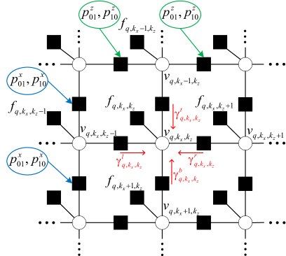
Figure 6: The internal structure of each sub-graph $\mathcal{G}_{q},q\in\mathbf{\Omega}$.

Then, the output message passed from the variable node $v_{q,k_{x},k_{z}}$ to the factor node $f_{q,k_{x},k_{z}}$ is expressed as

$$\gamma_{q,k_{x},k_{z}}^{l}= \frac{p_{11}^{z}\pi_{q,k_{x},k_{z}-1}^{in,1}\prod_{d\in\left\{l,t,b\right\}}\gamma_{q,k_{x},k_{z}-1}^{d}+p_{10}^{z}\pi_{q,k_{x},k_{z}-1}^{in,0}\prod_{d\in\left\{l,t,b\right\}}\left(1-\gamma_{q,k_{x},k_{z}-1}^{d}\right)}{\pi_{q,k_{x},k_{z}-1}^{in,1}\prod_{d\in\left\{l,t,b\right\}}\gamma_{q,k_{x},k_{z}-1}^{d}+\pi_{q,k_{x},k_{z}-1}^{in,0}\prod_{d\in\left\{l,t,b\right\}}\left(1-\gamma_{q,k_{x},k_{z}-1}^{d}\right)},$$ (46a)

$$\gamma_{q,k_{x},k_{z}}^{r}= \frac{p_{11}^{z}\pi_{q,k_{x},k_{z}+1}^{in,1}\prod_{d\in\left\{r,t,b\right\}}\gamma_{q_{i},k_{x},k_{z}+1}^{d}+p_{10}^{z}\pi_{q,k_{x},k_{z}+1}^{in,0}\prod_{n\in\left\{r,t,b\right\}}\left(1-\gamma_{q,k_{x},k_{z}+1}^{d}\right)}{\left(p_{11}^{z}+p_{01}^{z}\right)\pi_{q,k_{x},k_{z}+1}^{in,1}\prod_{d\in\left\{r,t,b\right\}}\gamma_{q,k_{x},k_{z}+1}^{d}+\left(p_{00}^{z}+p_{10}^{z}\right)\pi_{q,k_{x},k_{z}+1}^{in,0}\prod_{d\in\left\{r,t,b\right\}}\left(1-\gamma_{q,k_{x},k_{z}+1}^{d}\right)},$$ (46b)

$$\gamma_{q,k_{x},k_{z}}^{t}= \frac{p_{11}^{x}\pi_{q,k_{x}-1,k_{z}}^{in,1}\prod_{d\in\left\{l,r,t\right\}}\gamma_{q,k_{x}-1,k_{z}}^{d}+p_{10}^{x}\pi_{q,k_{x}-1,k_{z}}^{in,0}\prod_{d\in\left\{l,r,t\right\}}\left(1-\gamma_{q,k_{x}-1,k_{z}}^{d}\right)}{\pi_{q,k_{x}-1,k_{z}}^{in,1}\prod_{d\in\left\{l,r,t\right\}}\gamma_{q,k_{x}-1,k_{z}}^{d}+\pi_{q,k_{x}-1,k_{z}}^{in,0}\prod_{d\in\left\{l,r,t\right\}}\left(1-\gamma_{q,k_{x}-1,k_{z}}^{d}\right)},$$ (46c)

$$\gamma_{q,k_{x},k_{z}}^{b}= \frac{p_{11}^{x}\pi_{q,k_{x}+1,k_{z}}^{in,1}\prod_{d\in\left\{l,r,b\right\}}\gamma_{q,k_{x}+1,k_{z}}^{d}+p_{10}^{x}\pi_{q,k_{x}+1,k_{z}}^{in,0}\prod_{d\in\left\{l,r,b\right\}}\left(1-\gamma_{q,k_{x}+1,k_{z}}^{d}\right)}{\left(p_{11}^{x}+p_{01}^{x}\right)\pi_{q,k_{x}+1,k_{z}}^{in,1}\prod_{d\in\left\{l,r,b\right\}}\gamma_{q,k_{x}+1,k_{z}}^{d}+\left(p_{00}^{x}+p_{10}^{x}\right)\pi_{q,k_{x}+1,k_{z}}^{in,0}\prod_{d\in\left\{l,r,b\right\}}\left(1-\gamma_{q,k_{x}+1,k_{z}}^{d}\right)},$$ (46d)

 

$$\mathcal{V}_{q,k_{x},k_{z}}^{out}= \pi_{q,k_{x},k_{z}}^{out}\delta\left(v_{q,k_{x},k_{z}}-1\right)$$

$$+\left(1-\pi_{q,k_{x},k_{z}}^{out}\right)\delta\left(v_{q,k_{x},k_{z}}\right),$$ (47)

with

$$\pi_{q,k_{x},k_{z}}^{out}=\tfrac{\prod_{d\in\left\{l,r,t,b\right\}}\gamma_{q,k_{x},k_{z}}^{d}}{\prod_{d\in\left\{l,r,t,b\right\}}\gamma_{q,k_{x},k_{z}}^{d}+\prod_{d\in\left\{l,r,t,b\right\}}\left(1-\gamma_{q,k_{x},k_{z}}^{d}\right)}.$$

Now, we can obtain the posterior probability of $v_{q,k_{x},k_{z}}$ as

$$\hat{p}\left(v_{q,k_{x},k_{z}}=1\right)=\tfrac{\pi_{q,k_{x},k_{z}}^{in,1}\pi_{q,k_{x},k_{z}}^{out}}{\pi_{q,k_{x},k_{z}}^{in,1}\pi_{q,k_{x},k_{z}}^{out}+\pi_{q,k_{x},k_{z}}^{in,0}\left(1-\pi_{q,k_{x},k_{z}}^{out}\right)}.$$

Based on this, the posterior mean and variance of $v_{q,k_{x},k_{z}},q\in\mathbf{\Omega},\forall k_{x},k_{z}$ are computed by

$$\alpha_{q,k_{x},k_{z}}^{\textrm{B,post}}= \sum_{a\in\left\{0,1\right\}}\hat{p}\left(v_{q,k_{x},k_{z}}=a\right),$$ (48)

$$\beta_{q,k_{x},k_{z}}^{\textrm{B,post}}= \sum_{a\in\left\{0,1\right\}}\left(a-\alpha_{q,k_{x},k_{z}}^{\textrm{B,post}}\right)^{2}\hat{p}\left(v_{q,k_{x},k_{z}}=a\right).$$

Define $\boldsymbol{\alpha}_{k_{x},k_{z}}^{\textrm{B,post}}\triangleq\left[\alpha_{q,k_{x},k_{z}}^{\textrm{B,post}}\right]_{q\in\mathbf{\Omega}}$ and $\boldsymbol{\beta}_{k_{x},k_{z}}^{\textrm{B,post}}\triangleq\left[\beta{}_{q,k_{x},k_{z}}^{\textrm{B,post}}\right]_{q\in\mathbf{\Omega}}$, the extrinsic message passed from Module B to Module A is given by

$$\boldsymbol{\bar{\alpha}}_{k_{x},k_{z}}^{\textrm{A,pri}} =\boldsymbol{\bar{\beta}}_{k_{x},k_{z}}^{\textrm{A,pri}}\left(\boldsymbol{\alpha}_{k_{x},k_{z}}^{\textrm{B,post}}/\boldsymbol{\beta}_{k_{x},k_{z}}^{\textrm{B,post}}-\boldsymbol{\alpha}_{k_{x},k_{z}}^{\textrm{B,pri}}/\boldsymbol{\beta}_{k_{x},k_{z}}^{\textrm{B,pri}}\right),$$ (49)

$$\bar{\boldsymbol{\beta}}_{k_{x},k_{z}}^{\textrm{A,pri}} =1/\left(1/\boldsymbol{\beta}_{k_{x},k_{z}}^{\textrm{B,post}}-1/\boldsymbol{\beta}_{k_{x},k_{z}}^{\textrm{B,pri}}\right).$$

Notably, the update of the extrinsic variance will result in a negative $\bar{\beta}_{q,k_{x},k_{z}}^{\textrm{A,pri}}$ when $\beta_{q,k_{x},k_{z}}^{\textrm{B,post}}>\beta_{q,k_{x},k_{z}}^{\textrm{B,pri}}$, which is unreasonable. If the calculation of the posterior is exact, $\beta_{q,k_{x},k_{z}}^{\textrm{B,post}}>\beta_{q,k_{x},k_{z}}^{\textrm{B,pri}}$ will never happen since the posterior variance should be less than the prior variance. However, since sum-product is not exact for the 2D Markov prior whose factor graph has loops, this case may occur occasionally. In this case, we simply retain the previous values for $\alpha_{q,k_{x},k_{z}}^{\textrm{A,pri}}$and $\beta_{q,k_{x},k_{z}}^{\textrm{A,pri}}$. Such an approach is also employed in the conventional EP algorithm to ensure numerical stability [22]. In addition, a damping technique is usually used to smooth the update of extrinsic message [22, 39]:

$$\boldsymbol{\alpha}_{k_{x},k_{z}}^{\textrm{A,pri}}= \eta\bar{\boldsymbol{\alpha}}_{k_{x},k_{z}}^{\textrm{A,pri}}+\left(1-\eta\right)\boldsymbol{\alpha}_{k_{x},k_{z}}^{\textrm{A,pri}},$$ (50)

$$\boldsymbol{\beta}_{k_{x},k_{z}}^{\textrm{A,pri}}= \eta\bar{\boldsymbol{\beta}}_{k_{x},k_{z}}^{\textrm{A,pri}}+\left(1-\eta\right)\boldsymbol{\beta}_{k_{x},k_{z}}^{\textrm{A,pri}},$$

where $\eta\in\left(0,1\right)$ is a damping factor. The damping in (50) makes the structured EP more robust with improved stability and convergence properties.

Finally, we update the MAP estimate of $\hat{\mathbf{V}}_{q},q\in\mathbf{\Omega}$ by a hard decision as

$$\hat{v}_{q,k_{x},k_{z}}=\begin{cases}1,&\hat{p}\left(v_{q,k_{x},k_{z}}=1\right)\geq 0.5,\\ 0,&\hat{p}\left(v_{q,k_{x},k_{z}}=1\right)<0.5.\end{cases},\forall k_{x},k_{z}.$$ (51)

IV-D Gradient Ascent (Grid Update Module)

Based on $\hat{\boldsymbol{x}}$ and $\hat{\gamma}$ obtained in (37) and $\hat{\mathbf{V}}$ obtained in (51), the logarithmic posterior function is expressed as

$$\mathcal{L}\left(\boldsymbol{\Xi}\right) \triangleq\ln p\left(\boldsymbol{y}\mid\hat{\mathbf{V}},\hat{\boldsymbol{x}},\hat{\gamma};\boldsymbol{\Xi}\right)+\ln\left(\hat{\mathbf{V}},\hat{\boldsymbol{x}},\hat{\gamma}\right)-\ln\left(\boldsymbol{y}\right)$$

$$=-\hat{\gamma}\left\|\boldsymbol{y}-\left[\mathbf{A}\left(\boldsymbol{\Xi}\right)\varodot\mathbf{U}\left(\hat{\mathbf{V}}\right)\right]\hat{\boldsymbol{x}}\right\|^{2}+C,$$ (52)

where $C$ is a constant. It is difficult to find the optimal $\boldsymbol{\boldsymbol{\Xi}}$ that maximizes $\mathcal{L}\left(\boldsymbol{\Xi}\right)$ since $\mathcal{L}\left(\boldsymbol{\Xi}\right)$ is non-concave w.r.t. $\boldsymbol{\Xi}$. In this case, a gradient ascent approach is usually employed to update $\boldsymbol{\Xi}$. Specifically, in the $i\textrm{-th}$ iteration, the angle and distance parameters are updated as

$$\hat{\boldsymbol{\vartheta}}^{\left(i\right)} =\hat{\boldsymbol{\vartheta}}^{\left(i-1\right)}+\epsilon_{1}^{\left(i\right)}\nabla_{\boldsymbol{\vartheta}}\mathcal{L}\left(\boldsymbol{\vartheta},\boldsymbol{\hat{\phi}}^{\left(i-1\right)},\hat{\boldsymbol{r}}^{\left(i-1\right)}\right)\mid_{\boldsymbol{\vartheta}=\hat{\boldsymbol{\vartheta}}^{\left(i-1\right)}},$$

$$\boldsymbol{\hat{\phi}}^{\left(i\right)} =\boldsymbol{\hat{\phi}}^{\left(i-1\right)}+\epsilon_{2}^{\left(i\right)}\nabla_{\boldsymbol{\phi}}\mathcal{L}\left(\hat{\boldsymbol{\vartheta}}^{\left(i\right)},\boldsymbol{\hat{\phi}},\hat{\boldsymbol{r}}^{\left(i-1\right)}\right)\mid_{\boldsymbol{\phi}=\boldsymbol{\hat{\phi}}^{\left(i-1\right)}},$$

$$\frac{1}{\boldsymbol{\hat{r}}^{\left(i\right)}} =\frac{1}{\boldsymbol{\hat{r}}^{\left(i-1\right)}}+\epsilon_{3}^{\left(i\right)}\nabla_{\boldsymbol{r}}\mathcal{L}\left(\hat{\boldsymbol{\vartheta}}^{\left(i\right)},\boldsymbol{\hat{\phi}}^{\left(i\right)},\boldsymbol{r}\right)\mid_{\boldsymbol{r}=\hat{\boldsymbol{r}}^{\left(i-1\right)}},$$ (53)

where $\epsilon_{1}^{\left(i\right)}$, $\epsilon_{2}^{\left(i\right)}$, and $\epsilon_{3}^{\left(i\right)}$ are step sizes determined by the Armijo rule. Note that we update $\frac{1}{\hat{\boldsymbol{r}}}$ instead of $\hat{\boldsymbol{r}}$ since $\frac{1}{r}$ is uniformly sampled in the polar domain [12].

IV-E Complexity Analysis

We summarize the proposed alternating MAP framework in Algorithm 1. In the channel estimation module, the complicated matrix inverse is avoid, and only some matrix-vector product and diagonal matrix inverse are needed, whose complexity is $\mathcal{O}\left(MQ\right)$ per iteration. In the VR detection module, the complexity of the LMMSE estimator in Module A is dominated by $K$ small-scale matrix inverse operations, whose complexity is $\mathcal{O}\left(K\left|\mathbf{\Omega}\right|^{3}\right)$ per iteration. And the message passing in Module B is linear complexity. In the grid update module, the complexity of the gradient calculation is $\mathcal{O}\left(Q^{2}\right)$. Denote the inner iteration number of the IF-VBI and the structured EP as $I_{1}$ and $I_{2}$, respectively, the overall complexity of the alternating MAP is $\mathcal{O}\left(I_{1}MQ+I_{2}K\left|\mathbf{\Omega}\right|^{3}+Q^{2}\right)$ per outer iteration.

Algorithm 1 The alternating MAP algorithm

Input: $\boldsymbol{y}$, initial grid $\boldsymbol{\bar{\Xi}}$, inner iteration number $I_{1},I_{2}$, outer iteration number $I_{out}$.

Output: $\hat{\boldsymbol{x}}$, $\hat{\mathbf{V}}$, and $\hat{\boldsymbol{\Xi}}$.

1:  Initialize: $\hat{\mathbf{V}}_{q}=\mathbf{1}_{K_{x}\times K_{z}},\forall q$, $\hat{\boldsymbol{\Xi}}=\bar{\mathbf{\Xi}}$.

2:  for ${\color[rgb]{0,0,1}{\color[rgb]{0,0,0}i_{out}=1,\cdots,I_{out}}}$ do

3:     % Channel estimation module: IF-VBI estimator

4:     Initialize: $T=\lambda_{\textrm{max}}\left(\mathbf{F}^{H}\mathbf{F}\right)$, $\boldsymbol{z}=\mathbf{F}^{H}\boldsymbol{y}$.

5:     for ${\color[rgb]{0,0,1}{\color[rgb]{0,0,0}i_{1}=1,\cdots,I_{1}}}$ do

6:        Majorization: update each variational distribution $q\left(\mathbf{\Theta}^{k}\right)$, using (29) and (33).

7:        Minimization: update the parameter $\boldsymbol{z}$, using (36).

8:     end for

9:     Update $\hat{\boldsymbol{x}}$ and $\hat{\gamma}$, using (37).

10:     % VR detection module: structured EP

11:     for ${\color[rgb]{0,0,1}{\color[rgb]{0,0,0}i_{2}=1,\cdots,I_{2}}}$ do

12:        % Module A: LMMSE estimator

13:        Update $\boldsymbol{\alpha}_{k_{x},k_{z}}^{\textrm{A,post}}$ and $\boldsymbol{\beta}_{k_{x},k_{z}}^{\textrm{A,post}}$, using (41).

14:        Calculate the extrinsic message from Module A to B based on (42).

15:        % Module B: 2D-Markov-MMSE estimator

16:        Perform message passing over each sub-graph, using (45) and (47).

17:        Update $\boldsymbol{\alpha}_{k_{x},k_{z}}^{\textrm{B,post}}$ and $\boldsymbol{\beta}_{k_{x},k_{z}}^{\textrm{B,post}}$, using (48).

18:        Calculate the extrinsic message from Module B to A based on (49) and (50).

19:     end for

20:     Update $\hat{\mathbf{V}}$, using (51).

21:     % Grid update module: gradient ascent

22:     Update $\hat{\boldsymbol{\Xi}}$ ($\hat{\boldsymbol{\vartheta}},\boldsymbol{\hat{\phi}},\hat{\boldsymbol{r}}$), using (53).

23:  end for

24:  Output $\hat{\boldsymbol{x}}$, $\hat{\mathbf{V}}$, and $\hat{\boldsymbol{\Xi}}$.

V Simulation Results

In this section, we evaluate the performance of our proposed method through adequate numerical simulations. Some baselines and the proposed method are summarized below.

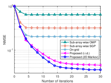
Figure 7: Convergence behavior: NMSE of channel estimation with respect to the number of iterations when $\textrm{SNR}=-4\ \textrm{dB}$.

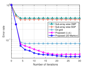
Figure 8: Convergence behavior: error rate of VR detection with respect to the number of iterations when $\textrm{SNR}=-4\ \textrm{dB}$.

• Sub-array-wise OMP [16, 12, 19]: Each sub-array uses the OMP algorithm to estimate each sub-channel independently and updates the polar-domain grid parameters via gradient ascent.

• Sub-array-wise stochastic gradient pursuit (SGP) [40]: Each sub-array employs the SGP algorithm to estimate each sub-channel independently and refines the polar-domain grid parameters via gradient ascent.

• On-grid: It is the proposed alternating MAP algorithm based on the on-grid model, i.e., the polar-domain grid is fixed.

• Proposed (i.i.d.): It is the proposed algorithm with the i.i.d. Bernoulli prior for VRs. In this case, the VR detection module is the conventional EP algorithm [22].

• Proposed (2D Markov): It is the proposed algorithm with the 2D Markov prior for VRs.

• Genie-aided: It is the proposed algorithm when the distance and angle parameters are assumed to be known perfectly. And thus, it is a performance upper bound for the proposed method.

The parameters of the considered XL-MIMO system are set as follows: the number of the UPA antennas is $M_{x}=256$ and $M_{z}=8$; the UPA is partitioned into $K_{x}\times K_{z}=16\times 2$ small-scale sub-UPAs, and the number of the sub-UPA antennas is $N_{x}=16$ and $N_{z}=4$; the carrier frequency is $30\ \textrm{GHz}$, while the Rayleigh distance is $325.37\ \textrm{m}$. We consider a multipath channel model, where the number of paths is set to $L=4$. The whole channel is spatial non-stationary, while each sub-channel corresponding to each sub-array is assumed to be spatial stationary. The visibility probability of the scatterers is $\kappa=0.5$, and the VR of the scatterers concentrates on a few clusters. We use the “COST 2100 Channel Model” toolbox to generate the spatial non-stationary XL-MIMO channel [41]. The normalized mean square error (NMSE) is used as the performance metric for channel estimation. And the error rate is used to measure the performance of VR detection, which is defined as

$$\textrm{Error\ rate}\triangleq\frac{\sum_{l=1}^{L}\left|\mathbf{V}_{l}-\hat{\mathbf{V}}_{q_{l}}\right|}{K_{x}K_{z}L}\leq 1,$$ (54)

where $q_{l}$ is the index of the polar-domain grid point nearest to the true position of scatterer $l$.

V-A Convergence Behavior

In Fig. 8 and Fig. 8, we compare the convergence behavior of different methods in terms of channel estimation NMSE and VR detection error rate, respectively. The convergence speed of the sub-array-wise OMP and SGP is very quick, but both of them converge to a very poor stationary point. By contrast, the on-grid method (the proposed algorithm based on the on-grid model) can find a better stationary point than the sub-array-wise methods and achieve similar convergence speed. Besides, the convergence behavior of the proposed algorithm with the i.i.d. prior and the 2D Markov prior is similar. Both of them converge within $20$ iterations, and they achieve better steady-state performance than the on-grid method, which shows the advantage of the designed dynamic polar-domain grid over the fixed grid. Moreover, the proposed algorithm with the 2D Markov prior has a performance gain over the same algorithm with the i.i.d. prior after convergence. This is because the 2D Markov prior can fully exploit the 2D clustered sparsity of VRs to enhance the performance.

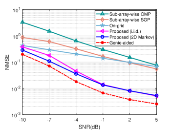
Figure 9: NMSE of channel estimation versus SNR.

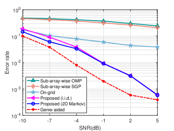
Figure 10: Error rate of VR detection versus SNR.

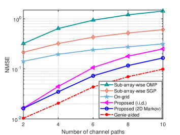
Figure 11: NMSE of channel estimation versus the number of channel paths when $\textrm{SNR}=-4\ \textrm{dB}$.

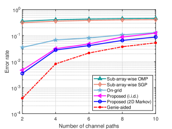
Figure 12: Error rate of VR detection versus the number of channel paths when $\textrm{SNR}=-4\ \textrm{dB}$.

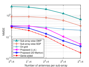
Figure 13: NMSE of channel estimation versus the number of antennas per sub-array. We set $\textrm{SNR}=-4\ \textrm{dB}$ and $N_{z}=4$.

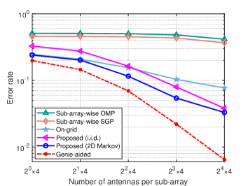
Figure 14: Error rate of VR detection versus the number of antennas per sub-array. We set $\textrm{SNR}=-4\ \textrm{dB}$ and $N_{z}=4$.

V-B Impact of SNR

In Fig. 10 and Fig. 10, we evaluate the performance of channel estimation and VR detection against SNR, respectively. As can be seen, the performance of all methods improves as the SNR increases. The sub-array-wise methods works poorly since they ignore the fact that sub-channels share some common scatterers as well as the associated channel parameters. Besides, the proposed algorithm based on the dynamic grid has a significant performance gain over the on-grid method, which verifies that the dynamic polar-domain grid greatly improves the performance. Furthermore, in the low SNR regions ($-10\ \textrm{dB}\sim-4\ \textrm{dB}$), the proposed algorithm with the 2D Markov prior works better than the proposed algorithm with the i.i.d. prior, which indicates that 2D Markov model can capture the the 2D clustered sparse structure well. However, the performance gain disappears in the high SNR regions. This is because the observation information is enough to estimate the channel and VRs accurately when the SNR is high. In this case, the prior information contributes little to the performance of the algorithm. Finally, the performance of the proposed algorithm with the 2D Markov prior is close to the genie-aided method, which indicates that the dynamic grid parameters can be refined well via gradient ascent.

V-C Impact of Number of Channel Paths

In Fig. 12 and Fig. 12, we focus on how the number of channel paths affects the performance of different methods when $\textrm{SNR}=-4\ \textrm{dB}$. We vary the number of channel paths from $L=2$ to $L=10$. There are more non-zero channel parameters that need to be estimated when the number of paths is larger. As a result, the performance of the methods decreases gradually as the number of paths increases. Again, we find that the proposed algorithm with the 2D Markov prior outperforms other baseline methods. In addition, the performance gap between the proposed algorithm with the 2D Markov prior and the i.i.d. prior is more obvious when the number of paths is large. In this case, the 2D Markov prior information plays a key role in the algorithm.

V-D Impact of Number of Antennas Per Sub-array

Fig. 14 and Fig. 14 plot the NMSE of channel estimation and error rate of VR detection against the number of antennas per sub-array, respectively. We keep $N_{z}=4$ and vary $N_{x}$ from $2^{0}$ to $2^{4}$. Note that the sub-array is spatial stationary when $N_{x}\leq 16$ and $N_{z}\leq 4$, and a $16\times 4$ sub-UPA is the largest unit keeping spatial stationary. It can be seen that with the increase in $N_{x}$, the NMSE and VR error rate of the methods reduced. This is because different antennas in a same sub-array share the same VRs. As a result, as $N_{x}$ increases, the sub-array-specific sparsity increases, which the proposed method fully exploit. We also notice that for all sub-array sizes, the proposed algorithm with the 2D Markov prior works better than baselines.

VI Conclusions

We propose a joint VR detection and channel estimation method for XL-MIMO systems. Based on the polar-domain sparse representation of the XL-MIMO channel, we use a hierarchical sparse prior model to capture the sparsity of the channel vector. Besides, a 2D Markov model is designed to fully exploit the 2D clustered sparsity of VRs. Based on these, the considered problem is formulated as a MAP estimation problem. A novel alternating MAP framework is developed to solve the problem by combining the IF-VBI estimator, structured EP algorithm, and gradient ascent approach. Three basic modules of the proposed alternating MAP framework work alternatively to estimate the polar-domain channel vector, detect the VRs, and refine the dynamic grid parameters. Simulations verify that our proposed method outperforms baselines in terms of both channel estimation and VR detection.

In future work, we will extend the proposed method to more challenging scenarios, such as channel tracking with multiple time slots, multiple users with pilot contamination, and the receiver with a hybrid beamforming (HBF) architecture.

References

• [1] T. S. Rappaport, Y. Xing, O. Kanhere, S. Ju, A. Madanayake, S. Mandal, A. Alkhateeb, and G. C. Trichopoulos, “Wireless communications and applications above 100 GHz: Opportunities and challenges for 6G and beyond,” IEEE Access, vol. 7, pp. 78 729–78 757, 2019.
• [2] S. Hu, F. Rusek, and O. Edfors, “Beyond massive MIMO: The potential of data transmission with large intelligent surfaces,” IEEE Trans. Signal Process., vol. 66, no. 10, pp. 2746–2758, 2018.
• [3] H. Elayan, O. Amin, B. Shihada, R. M. Shubair, and M.-S. Alouini, “Terahertz band: The last piece of RF spectrum puzzle for communication systems,” IEEE Open J. Commun. Soc., vol. 1, pp. 1–32, 2020.
• [4] Y. Liu, Z. Wang, J. Xu, C. Ouyang, X. Mu, and R. Schober, “Near-field communications: A tutorial review,” IEEE Open J. Commun. Soc., vol. 4, pp. 1999–2049, 2023.
• [5] E. D. Carvalho, A. Ali, A. Amiri, M. Angjelichinoski, and R. W. Heath, “Non-stationarities in extra-large-scale massive MIMO,” IEEE Wireless Commun., vol. 27, no. 4, pp. 74–80, 2020.
• [6] Z. Yuan, J. Zhang, Y. Ji, G. F. Pedersen, and W. Fan, “Spatial non-stationary near-field channel modeling and validation for massive MIMO systems,” IEEE Trans. Antennas Propag., vol. 71, no. 1, pp. 921–933, 2023.
• [7] Y. Zhu, H. Guo, and V. K. N. Lau, “Bayesian channel estimation in multi-user massive MIMO with extremely large antenna array,” IEEE Trans. Signal Process., vol. 69, pp. 5463–5478, 2021.
• [8] A. Tang, J.-b. Wang, Y. Pan, W. Zhang, Y. Chen, Y. Hongkang, and R. C. d. Lamare, “Joint visibility region and channel estimation for extremely large-scale MIMO systems,” [Online]. Available: https://arxiv.org/abs/2311.09490.
• [9] J. Lee, G.-T. Gil, and Y. H. Lee, “Channel estimation via orthogonal matching pursuit for hybrid MIMO systems in millimeter wave communications,” IEEE Trans. Commun., vol. 64, no. 6, pp. 2370–2386, 2016.
• [10] A. Liu, V. K. N. Lau, and W. Dai, “Exploiting burst-sparsity in massive MIMO with partial channel support information,” IEEE Trans. Wireless Commun., vol. 15, no. 11, pp. 7820–7830, 2016.
• [11] L. Chen, A. Liu, and X. Yuan, “Structured turbo compressed sensing for massive MIMO channel estimation using a Markov prior,” IEEE Trans. Veh. Technol., vol. 67, no. 5, pp. 4635–4639, 2018.
• [12] M. Cui and L. Dai, “Channel estimation for extremely large-scale MIMO: Far-field or near-field?” IEEE Trans. Commun., vol. 70, no. 4, pp. 2663–2677, 2022.
• [13] X. Zhang, H. Zhang, and Y. C. Eldar, “Near-field sparse channel representation and estimation in 6G wireless communications,” IEEE Trans. Commun., vol. 72, no. 1, pp. 450–464, 2024.
• [14] S. Yang, C. Xie, W. Lyu, B. Ning, Z. Zhang, and C. Yuen, “Near-field channel estimation for extremely large-scale reconfigurable intelligent surface (XL-RIS)-aided wideband mmwave systems,” [Online]. Available: https://arxiv.org/abs/2304.00440.
• [15] Z. Lu, Y. Han, S. Jin, and M. Matthaiou, “Near-field localization and channel reconstruction for ELAA systems,” IEEE Trans. Wireless Commun., pp. 1–1, 2023.
• [16] Y. Han, S. Jin, C.-K. Wen, and X. Ma, “Channel estimation for extremely large-scale massive MIMO systems,” IEEE Wireless Commun. Lett., vol. 9, no. 5, pp. 633–637, 2020.
• [17] Y. Han, S. Jin, C.-K. Wen, and T. Q. S. Quek, “Localization and channel reconstruction for extra large RIS-assisted massive MIMO systems,” IEEE J. Sel. Topics Signal Process., vol. 16, no. 5, pp. 1011–1025, 2022.
• [18] H. Iimori, T. Takahashi, K. Ishibashi, G. T. F. de Abreu, D. González G., and O. Gonsa, “Joint activity and channel estimation for extra-large MIMO systems,” IEEE Trans. Wireless Commun., vol. 21, no. 9, pp. 7253–7270, 2022.
• [19] Y. Chen and L. Dai, “Non-stationary channel estimation for extremely large-scale MIMO,” IEEE Trans. Wireless Commun., pp. 1–1, 2023.
• [20] H. Duan, L. Yang, J. Fang, and H. Li, “Fast inverse-free sparse Bayesian learning via relaxed evidence lower bound maximization,” IEEE Signal Process. Lett., vol. 24, no. 6, pp. 774–778, 2017.
• [21] W. Xu, Y. Xiao, A. Liu, M. Lei, and M.-J. Zhao, “Joint scattering environment sensing and channel estimation based on non-stationary Markov random field,” IEEE Trans. Wireless Commun., vol. 23, no. 5, pp. 3903–3917, 2024.
• [22] J. Céspedes, P. M. Olmos, M. Sánchez-Fernández, and F. Perez-Cruz, “Expectation propagation detection for high-order high-dimensional MIMO systems,” IEEE Trans. Commun., vol. 62, no. 8, pp. 2840–2849, 2014.
• [23] D. Starer and A. Nehorai, “Passive localization of near-field sources by path following,” IEEE Trans. Signal Process., vol. 42, no. 3, pp. 677–680, 1994.
• [24] K. T. Selvan and R. Janaswamy, “Fraunhofer and Fresnel distances: Unified derivation for aperture antennas,” IEEE Antennas Propag. Mag., vol. 59, no. 4, pp. 12–15, 2017.
• [25] E. Fornasini, “2D Markov chains,” Linear Algebra Appl., vol. 140, pp. 101–127, 1990.
• [26] S. Jiang, X. Yuan, X. Wang, C. Xu, and W. Yu, “Joint user identification, channel estimation, and signal detection for grant-free NOMA,” IEEE Trans. Wireless Commun., vol. 19, no. 10, pp. 6960–6976, 2020.
• [27] W. Yan and X. Yuan, “Semi-blind channel-and-signal estimation for uplink massive MIMO with channel sparsity,” IEEE Access, vol. 7, pp. 95 008–95 020, 2019.
• [28] M. E. Tipping, “Sparse Bayesian learning and the relevance vector machine,” J. Mach. Learn. Res., vol. 1, no. 3, pp. 211–244, 2001.
• [29] S. Ji, Y. Xue, and L. Carin, “Bayesian compressive sensing,” IEEE Trans. Signal Process., vol. 56, no. 6, pp. 2346–2356, 2008.
• [30] D. G. Tzikas, A. C. Likas, and N. P. Galatsanos, “The variational approximation for Bayesian inference,” IEEE Signal Process. Mag., vol. 25, no. 6, pp. 131–146, 2008.
• [31] A. Liu, G. Liu, L. Lian, V. K. N. Lau, and M.-J. Zhao, “Robust recovery of structured sparse signals with uncertain sensing matrix: A Turbo-VBI approach,” IEEE Trans. Wireless Commun., vol. 19, no. 5, pp. 3185–3198, 2020.
• [32] A. Liu, L. Lian, V. Lau, G. Liu, and M.-J. Zhao, “Cloud-assisted cooperative localization for vehicle platoons: A turbo approach,” IEEE Trans. Signal Process., vol. 68, pp. 605–620, 2020.
• [33] W. Xu, A. Liu, B. Zhou, and M.-j. Zhao, “Successive linear approximation VBI for joint sparse signal recovery and dynamic grid parameters estimation,” [Online]. Available: https://arxiv.org/pdf/2307.09149.
• [34] M. Bayati and A. Montanari, “The dynamics of message passing on dense graphs, with applications to compressed sensing,” IEEE Trans. Inf. Theory, vol. 57, no. 2, pp. 764–785, 2011.
• [35] G. Parisi and R. Shankar, “Statistical field theory,” 1988.
• [36] L. Cheng, C. Xing, and Y.-C. Wu, “Irregular array manifold aided channel estimation in massive MIMO communications,” IEEE J. Sel. Topics Signal Process., vol. 13, no. 5, pp. 974–988, 2019.
• [37] Y. Sun, P. Babu, and D. P. Palomar, “Majorization-minimization algorithms in signal processing, communications, and machine learning,” IEEE Trans. Signal Process., vol. 65, no. 3, pp. 794–816, 2017.
• [38] F. Kschischang, B. Frey, and H.-A. Loeliger, “Factor graphs and the sum-product algorithm,” IEEE Trans. Inf. Theory, vol. 47, no. 2, pp. 498–519, 2001.
• [39] K. Pratik, B. D. Rao, and M. Welling, “RE-MIMO: Recurrent and permutation equivariant neural MIMO detection,” IEEE Trans. Signal Process., vol. 69, pp. 459–473, 2021.
• [40] Y.-M. Lin, Y. Chen, N.-S. Huang, and A.-Y. Wu, “Low-complexity stochastic gradient pursuit algorithm and architecture for robust compressive sensing reconstruction,” IEEE Trans. Signal Process., vol. 65, no. 3, pp. 638–650, 2017.
• [41] J. Flordelis, X. Li, O. Edfors, and F. Tufvesson, “Massive MIMO extensions to the COST 2100 channel model: Modeling and validation,” IEEE Trans. Wireless Communs., vol. 19, no. 1, pp. 380–394, 2020.