Bayesian Multilevel Compositional Data Analysis:
Introduction, Evaluation, and Application

Abstract

Multilevel compositional data commonly occur in various fields, particularly in intensive, longitudinal studies using ecological momentary assessments. Examples include data repeatedly measured over time that are non-negative and sum to a constant value, such as sleep-wake movement behaviours in a 24-hour day. This article presents a novel methodology for analysing multilevel compositional data using a Bayesian inference approach. This method can be used to investigate how reallocation of time between sleep-wake movement behaviours may be associated with other phenomena (e.g., emotions, cognitions) at a daily level. We explain the theoretical details of the data and the models, and outline the steps necessary to implement this method. We introduce the R package multilevelcoda to facilitate the application of this method and illustrate using a real data example. An extensive parameter recovery simulation study verified the robust performance of the method. Across all simulation conditions investigated in the simulation study, the model had minimal convergence issues (convergence rate $>$ 99%) and achieved excellent quality of parameter estimates and inference, with an average bias of 0.00 (range -0.09, 0.05) and coverage of 0.95 (range 0.93, 0.97). We conclude the article with recommendations on the use of the Bayesian compositional multilevel modelling approach, and hope to promote wider application of this method to answer robust questions using the increasingly available data from intensive, longitudinal studies.
Translational Abstract
In intensive, longitudinal studies, researchers often seek to understand how behaviours, emotion, and cognition interact in everyday life. When movement behaviours, such as sleep, physical activity, and sedentary behaviour, are repeatedly measured over time, they have a complex multilevel compositional structure. Therefore, analyses must address their unique properties to produce analytically and practically meaningful insights. In this article, we present a novel methodology to analyse multilevel compositional data using Bayesian inference. We describe the data structure and outline the steps necessary to implement this method. To facilitate its practical application, we introduce an R package multilevelcoda and demonstrate how to conduct this analysis and interpret the results in a real data application. We also verify the performance of this method through a simulation study. Across the tested conditions, the model had minimal convergence issues and produced unbiased parameter estimates and valid inferences. This method is recommended for analysing data with a multilevel compositional structure, such as daily movement behaviours. With the growing data availability from wearable devices and EMAs in psychological research, we encourage the research community to apply this method in their own work to shed novel light on how reallocation of movement behaviours are associated with emotional experiences and cognitive processes in real life.

Across the fields of clinical and health science research, the rise of ecological momentary assessments (EMAs), wearable devices, daily-intensive longitudinal study designs, has enabled researchers to capture real-time phenomena, such as health behaviours, cognition and emotion, and how they interact in everyday life. In many contexts, data that are repeatedly measured have a complex multilevel compositional structure. Some examples of multilevel compositional data include 24-hour sleep-wake movement behaviours (e.g., time spent in behaviours like sleep, physical activity, and sedentary behaviour, during the 24-hour day), dietary behaviour (e.g., proportions of total caloric intake of macronutrients like proteins, fats and carbohydrates). These data are compositional, as they can be expressed as percentages (or proportions) or units that sum to a total constant value. They also have a multilevel structure, as they are usually measured across time and nested within clusters (e.g., daily measures of behaviours nested within people). Further, multilevel compositional data often contain two sources of variability: between-person (i.e., differences between individuals) and within-person (i.e., changes within individuals, such as the deviation from the average of an individual). These two unique processes open up an avenue to investigate beyond the average changes over time in a person and towards how the individual might fluctuate substantially around that mean, frequently using a multilevel modelling (MLM) approach.

Despite the growing evidence from EMA studies supporting the independent associations between daily movement behaviours and emotional experiences and cognitive processes [77], there is uncertainty about how daily reallocation of time across behaviours are associated with these phenomena. Specifically, existing analyses often focus on one of the behaviour components and neglect the compositional and/or multilevel nature of movement behaviours. Due to the fixed 24 hours in a day, a person who increases time spent in one behaviour must compensate by decreasing time spent in one or more other behaviours. For example, they can only increase time spent in physical activity by spending less time in other behaviours (e.g., sleep, sedentary behaviour). This is illustrated in Figure 1. In epidemiological research, the compositional approach, particularly the compositional isotemporal substitution model [70, 69], has been increasingly employed to investigate how reallocation of one behaviour to another, while keeping the total time fixed, are associated with physical and mental health outcomes [78, 76, 75, 91]. Existing epidemiological studies are, however, often interested in outcomes that are stable over time (i.e., cross-sectional), such as incidence of diseases. In contrast, longitudinal studies using EMA designs often seek to identify the between- and within-person processes in the variable trajectories as they emerge across time. With the growing data availability from EMAs in psychological research, emerging advanced approaches that accommodate the theoretical properties of multilevel compositional data could, therefore, facilitate more conceptually and analytically meaningful analyses, leading to new health insights.

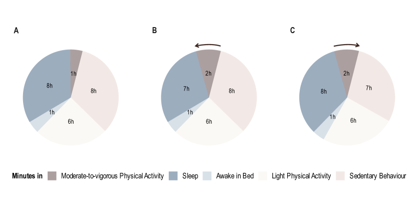
Figure 1: An example composition of time spent in movement behaviours of an individual is shown in Panel A. Due to the fixed 24-hour day, the individual can reallocate time across behaviours differently, but they must keep the total time fixed. They can increase an hour of moderate-to-vigorous physical activity at the expense of sleep (Panel B). Alternatively, they can increase an hour of moderate-to-vigorous physical activity at the expense of sedentary behaviour (Panel C).

Bayesian MLMs offer great flexibility in modelling statistical phenomena that exist in different levels. Although model estimation by Bayesian and frequentist approaches can include both population-level and group-level effects (also referred to as fixed and random effects), Bayesian MLMs have been increasingly employed due to their flexible model estimation and straightforward interpretation of results. Importantly, a fundamental aspect of Bayesian framework is quantifying uncertainty parameters and models using probability theory, which is not provided by frequentist approaches [74, 111]. Using Bayes’s theorem, the posterior distribution of any parameters can be derived to reflect the knowledge of the model (i.e., prior) and the observed data (i.e., likelihood). This allows for making probabilistic inferences about parameters (or their functions), enabling any post-hoc analyses involving calculated quantities to be directly and intuitively estimated. With the rapid development of software for Bayesian posterior sampling, including the probabilistic programming language Stan [68], easily accessible front-end R package brms [66] for model fitting with similar syntax to frequentist MLMs, [[, i.e., lme4,]]lme4, MLMs with complex data structure, such as multilevel composition, can be conceptually simple and computationally tractable in Bayesian framework.

In this paper, we present a novel methodology to model multilevel compositional data using Bayesian inference. This method can be used to address the interdependence of day-to-day movement behaviour composition and investigate how reallocation of movement behaviours may be associated with other phenomena at a daily level. We start by describing the structure of multilevel compositional data and the model specification, with a focus on models with compositional variables as predictors at both between- and within-person levels. To facilitate the implementation of this approach in a robust and principled workflow, we introduce the R package multilevelcoda [84, 83] and present its applications on a data set with daily repeated measures. We then use the results from the real data application as a starting point of a simulation study to assess the accuracy and precision of parameter estimates. We conclude the paper with a discussion on the use of this approach and recommendations on its practical applications.

1 Multilevel Compositional Data

Detailed structure of single-level compositional data and the relevant transformations have been described previously [105, 70, 101]. Here, we focus on the compositional data with multilevel structure, considering both the between (i.e., cluster-specific mean) and within (i.e., mean-centered deviate) levels, and two-level data hierarchy (i.e., daily observations nested within people).

For $d=1,\ldots,D$ part composition of $j=1,\ldots,J$ individuals across $i=1,\ldots,I$ time points, a multilevel composition is defined as a vector of $D$ positive components that sum to a constant $\kappa$, observed at the $i^{\text{th}}$ time point for the $j^{\text{th}}$ person. We denote the multilevel composition and its between- and within-person components as

$$\boldsymbol{x}_{ij} =(x_{1ij},x_{2ij},\ldots,x_{Dij}),\hskip 2.84544pt\text{where}\hskip 2.84544pt\sum_{i=1}^{D}x_{i}=\kappa$$

$$=\mathcal{C}\begin{pmatrix}x{{}^{(b)}_{1\boldsymbol{\cdot}j}}\boldsymbol{\cdot}x{{}^{(w)}_{1ij}},x{{}^{(b)}_{2\boldsymbol{\cdot}j}}\boldsymbol{\cdot}x{{}^{(w)}_{2ij}},\ldots,x{{}^{(b)}_{D\boldsymbol{\cdot}j}}\boldsymbol{\cdot}x{{}^{(w)}_{Dij}}\end{pmatrix}$$

$$=\boldsymbol{x}{{}^{(b)}_{\boldsymbol{\cdot}j}}\oplus\boldsymbol{x}{{}^{(w)}_{ij}}$$

in which superscripts $(b)$ and $(w)$ denote the between and within components of the composition, $\oplus$ is the perturbation operation on the simplex (closure operation applied to the element-wise product), and $\mathcal{C}\left(\boldsymbol{x}_{ij}\right)=\kappa\frac{\boldsymbol{x}}{}$ is the closure operation that ensures the compositional parts of the vector $\boldsymbol{x}_{ij}$ sum to the constant $\kappa$ [58]. The between- and within-person subcompositions are essentially compositions themselves as

$$\boldsymbol{x}{{}^{(b)}_{\boldsymbol{\cdot}j}} =\mathcal{C}\left(x{{}^{(b)}_{1\boldsymbol{\cdot}j}},x{{}^{(b)}_{2\boldsymbol{\cdot}j}},\ldots,x{{}^{(b)}_{D\boldsymbol{\cdot}j}}\right)\text{ and }$$

$$\boldsymbol{x}{{}^{(w)}_{ij}} =\mathcal{C}\left(x{{}^{(w)}_{1ij}},x{{}^{(w)}_{2ij}},\ldots,x{{}^{(w)}_{Dij}}\right).$$

Compositions are elements of the $D-$simplex ($\mathcal{S}^{D}$) whose properties are incompatible with standard mathematical operations (e.g., addition, multiplication) and statistical models (e.g., linear regression) [[, for detailed discussion on the properties of compositional data and their consequences, see]]Aitchison1994, Aitchison1986.

Compositional data analysis [[, CoDA;]]Aitchison1986, Pawlowsky2011 is a log-ratio analysis paradigm that utilises the relative information contained in compositional data. Although several transformations exist, isometric log-ratio ($ilr$) transformation [72] preserves the metric properties of the composition and accounts for the dependencies between its parts, so that standard statistical methods can be applied to the transformed data. This method involves transforming the $D-$part composition in the simplex ($\mathcal{S}^{D}$) to a set of $(D-1)-$dimension $ilr$ coordinates in the Euclidean space ($\mathbb{R}^{D-1}$) isometrically (i.e., preserving angles and distances). This isometry is constructed using the sequential binary partition (SBP), a $D\times(D-1)$ matrix that maps the $D$ compositional parts and their membership in the $(D-1)$ $ilr$ coordinates [71]. A SBP is obtained by first partitioning the compositional parts into two non-empty sets, where one set corresponds to the first $ilr$ coordinate’s numerator (coded as + 1) and the other set corresponds to the the first $ilr$ coordinate’s denominator (coded as -1), and where applicable, compositional part uninvolved in the $ilr$ are coded as 0. Using this principle, each of the previously constructed sets are recursively partitioned into two non-empty sets until no further partitions of the subcompositional parts are possible (after $D-1$ steps). $ilr$ coordinates can be interpreted as log ratio of the subcomposition in the numerator in relation to the subcomposition in the denominator. Although the order of parts in composition might be mathematically arbitrary, the SBP can be reconstructed to be intuitive and interpretable depending on application.

For a $D-$part composition $\boldsymbol{x}_{ij}\in\mathcal{S}^{D}$, the corresponding set of $D-1$ $ilr$ coordinates is $(z_{1ij},z_{2ij},\ldots,z_{(D-1)ij})=\boldsymbol{z}_{ij}\in\mathbb{R}^{D-1}$. The individual $k^{th}$ ($k=1,2,\ldots,D-1$) $ilr$ coordinate observed at time point $i$ for individual $j$, $z_{kij}$, can be expressed as

$$z_{kij}=\sqrt{\frac{r_{kij}s_{kij}}{r_{kij}\ +s_{kij}}}ln\left(\frac{\tilde{x}_{R_{kij}}}{\tilde{x}_{S_{kij}}}\right),\hskip 5.69046ptk=1,2,\ldots,D-1$$

where $\tilde{x}_{R_{kij}}$ and $\tilde{x}_{S_{kij}}$ are the geometric mean of a subcomposition in the numerator ($R_{kij}$) and the denominator ($S_{kij}$), respectively, with $r_{kij}$ and $s_{kij}$ being the size of the sets $R_{kij}$ and $S_{kij}$, respectively, and $\sqrt{\frac{r_{kij}s_{kij}}{r_{kij}\ +s_{kij}}}$ being a normalising constant.

As the $ilr$ coordinates exist in the Euclidean space $\mathbb{R}^{D-1}$, the decomposition of the $(D-1)-$dimension $ilr$ coordinates $\boldsymbol{z}_{ij}$ can be equivalently be decomposed into its between- and within-person components using the usual addition operation, that is

$$\boldsymbol{z}_{ij} =\left(z{{}^{(b)}_{1\boldsymbol{\cdot}j}}+z{{}^{(w)}_{1ij}},z{{}^{(b)}_{2\boldsymbol{\cdot}j}}+z{{}^{(w)}_{2ij}},\ldots,z{{}^{(b)}_{(D-1)\boldsymbol{\cdot}j}}+z{{}^{(w)}_{(D-1)ij}}\right)$$

$$=\boldsymbol{z}{{}^{(b)}_{\boldsymbol{\cdot}j}}+\boldsymbol{z}{{}^{(w)}_{ij}}$$

in which superscript ^(b) and ^(w) also denote the between and within components of the $ilr$ coordinates.

The $ilr$ coordinates are linearly independent multivariate real values. Therefore, once the multilevel composition has been re-expressed as a set of corresponding $ilr$ coordinates, they can be entered into standard statistical models [88], such as MLMs. Importantly, the $ilr$ transformation is invertible, meaning that the $ilr$ coordinates can be back-transformed via their $1-1$ relationship to the original composition for further investigation, if required [71].

2 Bayesian Compositional Multilevel Model

Our exposition of Bayesian inference will be kept to a minimum, given the rich and growing literature that offers methodological guidance on Bayesian analyses, including both introductions [80, 89] and advanced topics [74]. While several perspectives on Bayesian inference exist [[, for a review, see]]levy2023, our method adopts Bayesian approach due to its computational advantages when estimating complex models and the exchangeability assumption when building MLMs. We now explain the MLMs with compositional predictors and its associated post-hoc substitution models.

2.1 Bayesian Compositional Multilevel Model

We consider a continuous, normally distributed outcome variable observed at time point $i$ for individual $j$ as $y_{ij}$. within-person effects of a $D-$part composition (expressed as a set of $(D-1)-$dimension $ilr$ coordinates). A linear MLM of $y_{ij}$ with a varying intercept (also referred to as random intercept) can be written as

$$y_{ij}=\beta_{0j}+\overbrace{\sum_{k=1}^{D-1}\beta_{k}z^{(b)}_{k\boldsymbol{\cdot}j}}^{\text{between}}+\underbrace{\sum_{k=1}^{D-1}\beta_{(k+D-1)}z^{(w)}_{kij}}_{\text{within}}+\varepsilon_{ij}$$

where

$$\beta_{0j} =\gamma_{0}+u_{0j}$$

$$u_{0j} \sim\text{Normal}(0,\sigma^{2}_{u})$$

$$\varepsilon_{ij} \sim\text{Normal}(0,\sigma^{2}_{\varepsilon})$$

The between- and within-person components of the composition (expressed as a set of $ilr$ coordinates) are $z^{(b)}$ and $z^{(w)}$, with the subscripts denoting that the between component is unique to individual $j$ and the within component is unique to time $i$ for individual $j$. In this example model, all $z^{(b)}$ and $z^{(w)}$ are included as population-level effects, however, the $z^{(w)}$ can be allowed to vary if necessary. The between- and within-person effects of the $ilr$ coordinates are $\beta_{k}$ and $\beta_{k+D-1}$. Because each $ilr$ coordinate is decomposed into its between- and within-person components, for $D-1$ $ilr$ coordinates, the corresponding $\beta$ for them in the model is $2(D-1)$.

2.2 Bayesian Compositional Substitution Multilevel Model

Substitution analysis examines the expected difference in an outcome when a fixed unit $t$ of the composition is reallocated from one compositional component to another, while the other components remain fixed [69]. Given the different sources of variability in the composition, we can investigate the changes in an outcome associated with the reallocation of compositional parts at between-person (i.e., differences in composition between individuals) and within-person (i.e., changes in composition within an individual across time points) levels.

Table 1 outlines the steps for Bayesian compositional substitution MLM. A common reference composition is the compositional mean, thus, we briefly provide the notations for this scenario. When considering the compositional mean as the reference composition, there is no within-person variance at the compositional mean. Thus, the within-person component of the composition, $\boldsymbol{x}{{}^{(w)}_{0}}$, becomes the neutral element of the simplex, $\boldsymbol{1}_{D}=\mathcal{C}(1,1,\ldots,1)=(\kappa/D,\kappa/D,\ldots,\kappa/D)$. The reference composition and its corresponding $ilr$ transformation can be simplified to

$$\begin{aligned} \boldsymbol{x}_{0}&=\boldsymbol{x}^{(b)}_{0}\oplus\boldsymbol{1}_{D}=\boldsymbol{x}^{(b)}_{0}\\ \boldsymbol{z}_{0}&=\boldsymbol{z}_{0}^{(b)}+\boldsymbol{0}\hskip 8.5359pt=\boldsymbol{z}_{0}^{(b)}\end{aligned}.$$

The predicted outcome by the complete compositional predictor at the compositional mean, $\hat{y}_{0}$, become

$$\hat{y}_{0} =\hat{\beta}_{0j}+\sum_{k=1}^{D-1}\hat{\beta}_{k}z{{}^{(b)}_{k0}}+\sum_{k=1}^{D-1}\hat{\beta}_{(k+D-1)}z{{}^{(w)}_{k0}}$$

$$=\hat{\beta}_{0j}+\sum_{k=1}^{D-1}\hat{\beta}_{k}z{{}^{(b)}_{k0}}+0$$

$$=\hat{\beta}_{0j}+\sum_{k=1}^{D-1}\hat{\beta}_{k}z{{}^{(b)}_{k0}}$$

We follow with steps 5-8 as outlined in Table 1.

Table 1: Steps to Perform Bayesian Compositional Substitution Multilevel Model.

Step	Notation
1. Select a reference composition	$\boldsymbol{x}_{0}$
2. Decompose into its between and within levels	$\boldsymbol{x}{{}^{(b)}_{0}}$ and $\boldsymbol{x}{{}^{(w)}_{0}}$
3. Re-express composition as $ilr$ coordinates	$\boldsymbol{z}{{}^{(b)}_{k0}}$ and $\boldsymbol{z}{{}^{(w)}_{k0}}$
4. Estimate the outcome by the complete composition at the reference composition	$\hat{y}_{0}=\hat{\beta}_{0j}+\sum_{k=1}^{D-1}\hat{\beta}_{k}z{{}^{(b)}_{k0}}+\sum_{k=1}^{D-1}\hat{\beta}_{(k+D-1)}z{{}^{(w)}_{k0}}$
A. Between substitution
5A. Calculate the new composition for the reallocation at the between-person level	$\boldsymbol{x}{{}^{{(b)}^{\prime}}_{0}}$
6A. Re-express the new composition as $ilr$ coordinates	$\boldsymbol{z}{{}^{{(b)}^{\prime}}_{0}}$ and $\boldsymbol{z}{{}^{{(w)}^{\prime}}_{0}}$
7A. Estimate the outcome at the between-person reallocation	$\hat{y}^{(b)^{\prime}}_{0}=\hat{\beta}_{0j}+\sum_{k=1}^{D-1}\hat{\beta}_{k}z{{}^{(b)^{\prime}}_{k0}}+\sum_{k=1}^{D-1}\hat{\beta}_{(k+D-1)}z{{}^{(w)}_{k0}}$
8A. Estimate the difference in outcome between the between-person reallocation and the reference	$\Delta{\hat{y}^{(b)}}=\hat{y}^{(b)^{\prime}}_{0}-\hat{y}_{0}$
B. Within substitution
5B. Calculate the new composition for the reallocation at the within-person level	$\boldsymbol{x}{{}^{{(w)}^{\prime}}_{0}}$
6B. Re-express the new composition as $ilr$ coordinates	$\boldsymbol{z}{{}^{{(b)}^{\prime}}_{0}}$ and $\boldsymbol{z}{{}^{{(w)}^{\prime}}_{0}}$
7B. Estimate the outcome for the within-person reallocation	$\hat{y}^{(w)^{\prime}}_{0}=\hat{\beta}_{0j}+\sum_{k=1}^{D-1}\hat{\beta}_{k}z{{}^{(b)}_{k0}}+\sum_{k=1}^{D-1}\hat{\beta}_{(k+D-1)}z{{}^{{(w)}^{\prime}}_{k0}}$
8B. Estimate the difference in outcome between the within-person reallocation and the reference	$\Delta{\hat{y}^{(w)}}=\hat{y}^{(w)^{\prime}}_{0}-\hat{y}_{0}$

3 Software Implementation

We implemented this method in a free, open-source, easy-to use R package multilevelcoda [84, 83]. multilevelcoda is built on brms and Stan, which are easily accessible to lay users. The focus of multilevlecoda is on a streamlined and efficient workflow from dealing with raw multilevel compositional data, performing $ilr$ transformations, estimating Bayesian compositional MLMs and the associated subsitution models, and visualising final results (Figure 2).

Figure 2: Estimation Procedure using package multilevelcoda.

4 Illustrative Real Data Study

4.1 Aims

We demonstrated our approach in a real data application. The objectives of this study are to 1) examine the relationship between the 24-hour movement behaviours and sleepiness, and 2) investigate the changes in sleepiness associated with the change in movement behaviours at both between- and within-person levels.

4.2 Method

4.2.1 Data

The data come from three studies with similar daily intensive designs and repeated measures: Activity, Coping, Emotions, Stress, and Sleep (ACES. N = 187); Diet, Exercise, Stress, Emotions, Speech, and Sleep (DESTRESS, N = 78); and Stress and Health Study (SHS, N = 96). Study materials are available on the Open Science framework for ACES (https://doi.org/10.17605/OSF.IO/H5497), DESTRESS (https://doi.org/10.17605/OSF.IO/QM63W), and SHS (https://doi.org/10.17605/OSF.IO/TZ48Y). Details of the data collection have been described previously [81, 113]. This data set had the data structure found in typical applications of multilevel analysis in psychological research (i.e., daily observations of movement behaviours are nested within individuals). For the purposes of this illustration, we used the data of 345 healthy adults, from whom we have repeated measurements of sleepiness and five movement behaviours of total sleep time, time awake in bed, moderate-to-vigorous physical activity (MVPA), light physical activity (LPA), and sedentary behaviour (SB). Sleepiness was a single item and self-reported 3-4 times daily, which was averaged to obtain the average daily level of sleepiness. The five behaviours were recorded via an actigraph for 7-12 days and scored using the GGIR R package [107, 106, 108, 109, 92]. These data are available from the corresponding author upon request.

4.2.2 Analytical Approach

The movement behaviours make up of a 5-part composition ($D$ = 5), which corresponds to a 4-dimensional set of $ilr$ coordinates. Individuals with missing data and zero values of any behaviours were excluded, as missing data and zeros hamper the analysis of compositional data (as the $ilr$ transformation cannot compute 0s). The two sets of between- and within-person $ilr$ coordinates were constructed using a SBP that represents the relative information of compositional parts as follows:

$$z{{}^{(b)}_{1\boldsymbol{\cdot}j}} =\sqrt{\frac{6}{5}}ln\frac{(\text{Sleep}^{(b)}\cdot\text{Awake in Bed}^{(b)})^{\nicefrac{{1}}{{2}}}}{(\text{MVPA}^{(b)}\cdot\text{LPA}^{(b)}\cdot\text{SB}^{(b)})^{\nicefrac{{1}}{{3}}}}$$

$$z{{}^{(b)}_{2\boldsymbol{\cdot}j}} =\sqrt{\frac{1}{2}}ln\frac{\text{Sleep}^{(b)}}{\text{Awake in Bed}^{(b)}}$$

$$z{{}^{(b)}_{3\boldsymbol{\cdot}j}} =\sqrt{\frac{2}{3}}ln\frac{\text{MVPA}^{(b)}}{(\text{LPA}^{(b)}\cdot\text{SB}^{(b)})^{\nicefrac{{1}}{{2}}}}$$

$$z{{}^{(b)}_{4\boldsymbol{\cdot}j}} =\sqrt{\frac{1}{2}}ln\frac{\text{LPA}^{(b)}}{\text{SB}^{(b)}}$$

and

$$z{{}^{(w)}_{1ij}} =\sqrt{\frac{6}{5}}ln\frac{(\text{Sleep}^{(w)}\cdot\text{Awake in Bed}^{(w)})^{\nicefrac{{1}}{{2}}}}{(\text{MVPA}^{(w)}\cdot\text{LPA}^{(w)}\cdot\text{SB}^{(w)})^{\nicefrac{{1}}{{3}}}}$$

$$z{{}^{(w)}_{2ij}} =\sqrt{\frac{1}{2}}ln\frac{\text{Sleep}^{(w)}}{\text{Awake in Bed}^{(w)}}$$

$$z{{}^{(w)}_{3ij}} =\sqrt{\frac{2}{3}}ln\frac{\text{MVPA}^{(w)}}{(\text{LPA}^{(w)}\cdot\text{SB}^{(w)})^{\nicefrac{{1}}{{2}}}}$$

$$z{{}^{(w)}_{4ij}} =\sqrt{\frac{1}{2}}ln\frac{\text{LPA}^{(w)}}{\text{SB}^{(w)}}.$$

The $ilr$ coordinates represent the relative effects of behaviours (increasing some while at decreasing others), accounting for the constrained nature between behaviours within the 24-hour day. Specifically, across the between- and within-person levels, they represent the effects of (1) increasing sleep and time awake in bed while proportionally decreasing MVPA, LPA, and SB, (2) increasing sleep while proportionally decreasing time awake in bed, (3) increasing MVPA while proportionally decreasing LPA and SB, and (4) increasing LPA while proportionally decreasing SB.

We considered a Bayesian compositional MLM with a varying-intercept. The predictors are the 5-part movement composition, expressed as a total of 8 between- and within-person $ilr$ coordinates. The outcome of the model is next-day sleepiness. A varying-intercept by participants was included to account for non-independence. The model was fitted with weakly informative priors, 4 chains, and 4 cores, with 3000 iterations including 500 warmups (total of 10000 post-warmup draws), using CmdStanR [102] as back-end. We used weakly-informative priors, which play a minimal role in the computation of the posterior distribution, and maximise the influence of the data. For the population-level effects, student’s t distribution were used for the constant (i.e., fixed) intercept, and flat priors (improper priors over the reals) were used for the constant parameters of the predictors. Group-level effects also have their standard deviation parameters (i.e., varying intercept and residual), which were specified using student’s t distribution. The priors for the standard deviation parameters are restricted to be non-negative and have a half student-t prior with 3 degrees of freedom and a scale parameter that depends on the standard deviation of the outcome. These priors are only weakly informative, but provide some regularisation to improve convergence and sampling efficiency [67]. Prior information is given in Table 2.

Table 2: Priors Setting for Bayesian Compositional Multilevel Models.

	Parameter	Prior
Population-level
Intercept	$\gamma_{0}$	student_t(3, 2.6, 3.1)
1st between $ilr$	$\beta{z{{}^{(b)}_{1\boldsymbol{\cdot}j}}}$	flat
2nd between $ilr$	$\beta{z{{}^{(b)}_{2\boldsymbol{\cdot}j}}}$	flat
3rd between $ilr$	$\beta{z{{}^{(b)}_{3\boldsymbol{\cdot}j}}}$	flat
4th between $ilr$	$\beta{z{{}^{(b)}_{4\boldsymbol{\cdot}j}}}$	flat
1st within $ilr$	$\beta{z{{}^{(w)}_{1ij}}}$	flat
2nd within $ilr$	$\beta{z{{}^{(w)}_{2ij}}}$	flat
3rd within $ilr$	$\beta{z{{}^{(w)}_{3ij}}}$	flat
4th within $ilr$	$\beta{z{{}^{(w)}_{4ij}}}$	flat
Group-level
Intercept	$\sigma_{u}$	student_t(3, 0, 3.1)
Residual	$\sigma_{\varepsilon}$	student_t(3, 0, 3.1)

The Bayesian compositional substitution MLM was then conducted for both between- and within-person levels, examining the predicted change in sleepiness associated with the pairwise reallocation from 1 to 30 minutes between the composition of 24-hour movement behaviours.

Significance of individual parameters was assessed using the Bayesian 95% posterior credible interval, with 95% credible intervals (CIs) not containing 0 providing evidence for the probability that the true estimate would lie within the interval. All analyses were performed in R v4.3.1 [97], using package multilevelcoda v1.1.0 (model estimation, workflow outlined in Figure 2), brms [66], future [[, parallel processing,]]future, and ggplot2 [[, results visualisation,]]ggplot. All analysis code is available at: https://github.com/florale/multilevelcoda-sim.

4.3 Results

4.3.1 Bayesian Compositional Multilevel Model

Results from the MLM predicting next-day sleepiness from a 5-part composition are presented in Table 3, supporting the effects of all within-person $ilr$ coordinates (indicated by 95% CIs not containing 0s), but not any between-person $ilr$ coordinates (indicated by 95% CIs containing 0s). This demonstrated the relationships between movement behaviours and next-day sleepiness occurred only at within-person level, but not between-person level. Overall, the $1^{st}$ within-person $ilr$ coordinate (longer time spent on sleep behaviours than usual [sleep and time awake in bed], relative to wake behaviours [MVPA, LPA, and SB]) predicted -0.59 [95% CI -0.70, -0.49] lower next-day sleepiness. The $2^{nd}$ within-person $ilr$ coordinate (longer sleep than usual, relative to spending time staying awake in bed), also predicted lower -0.44 [95% CI -0.55, -0.34] next-day sleepiness. Similarly, the $3^{rd}$ within-person $ilr$ coordinate (higher-than-usual MVPA, relative to LPA and SB) and the $4^{th}$ within $ilr$ coordinate (higher-than-usual LPA relative to SB), predicted lower sleepiness (-0.27 [95% CI -0.39, -0.16] and -0.20 [95% CI -0.35, -0.06], respectively).

Table 3: Associations of the 24-hour Sleep-Wake Movement Behaviours and Sleepiness.

Parameter	Interpretation	Posterior mean and 95% credible intervals
Between-person level
$z^{(b)}_{1}$	Longer sleep and awake in bed, relative to MVPA, LPA, and SB	$\begin{matrix}0.16\\ [-0.15,0.46]\end{matrix}$
$z^{(b)}_{2}$	Longer sleep, relative to awake in bed	$\begin{matrix}-0.01\\ [-0.27,0.25]\end{matrix}$
$z^{(b)}_{3}$	Longer MVPA, relative to LPA and SB	$\begin{matrix}0.16\\ [-0.17,0.49]\end{matrix}$
$z^{(b)}_{4}$	Longer LPA, relative to SB	$\begin{matrix}0.04\\ [-0.36,0.43]\end{matrix}$
Within-person level
$z^{(w)}_{1}$	Longer-than-usual sleep and awake in bed, relative to MVPA, LPA, and SB on a given day	$\begin{matrix}-0.59^{\ast}\\ [-0.69,-0.49]\end{matrix}$
$z^{(w)}_{2}$	Longer-than-usual sleep, relative to awake in bed on a given day	$\begin{matrix}-0.44^{\ast}\\ [-0.55,-0.34]\end{matrix}$
$z^{(w)}_{3}$	Longer-than-usual MVPA, relative to LPA and SB on a given day	$\begin{matrix}-0.27^{\ast}\\ [-0.39,-0.16]\end{matrix}$
$z^{(w)}_{4}$	Longer-than-usual LPA, relative to SB within level on a given day	$\begin{matrix}-0.20^{\ast}\\ [-0.35,-0.06]\end{matrix}$

Notes. ^∗95% credible intervals not containing 0.

4.3.2 Bayesian Compositional Substitution Multilevel Model

Consistent with the main MLM, reallocation of time between movement behaviours predicted changes in sleepiness at the within-person level, but not the between-person level. Individuals slept longer-than-usual at the expense of any behaviours, except MVPA, at within level, experienced lower level of next-day sleepiness. However, when individuals sacrificed their sleep on a given day is for any other behaviours (i.e., including MVPA), they experienced a higher level of sleepiness. Additionally, individuals who spent longer time in LPA at the expense of time awake in bed on a given day, also experienced a higher level of sleepiness the next day, and vice versa. Results of the substitution model for 30-minute reallocation are in Table 4. For brevity, we presented only the significant results for the reallocation from 1 to 30 minutes of Sleep and Awake in bed, respectively, in Figure 3.

Table 4: Estimated Difference in Sleepiness Associated with Reallocation of 30 minutes Across Sleep-Wake Movement Behaviours.

	$\downarrow\text{Sleep}$	$\downarrow\text{Awake in bed}$	$\downarrow\text{MVPA}$	$\downarrow\text{LPA}$	$\downarrow\text{SB}$
Between-person level
$\uparrow\text{Sleep}$	-	$\begin{matrix}-0.05\\ [-0.15,0.05]\end{matrix}$	$\begin{matrix}-0.05\\ [-0.22,0.12]\end{matrix}$	$\begin{matrix}0.04\\ [-0.08,0.16]\end{matrix}$	$\begin{matrix}0.01\\ [-0.02,0.04]\end{matrix}$
$\uparrow\text{Awake in bed}$	$\begin{matrix}0.03\\ [-0.04,0.09]\end{matrix}$	-	$\begin{matrix}-0.02\\ [-0.20,0.17]\end{matrix}$	$\begin{matrix}0.07\\ [-0.06,0.20]\end{matrix}$	$\begin{matrix}0.04\\ [-0.02,0.10]\end{matrix}$
$\uparrow\text{MVPA}$	$\begin{matrix}0.02\\ [-0.08,0.13]\end{matrix}$	$\begin{matrix}-0.03\\ [-0.17,0.11]\end{matrix}$	-	$\begin{matrix}0.07\\ [-0.14,0.27]\end{matrix}$	$\begin{matrix}0.04\\ [-0.06,0.14]\end{matrix}$
$\uparrow\text{LPA}$	$\begin{matrix}-0.03\\ [-0.13,0.06]\end{matrix}$	$\begin{matrix}-0.08\\ [-0.21,0.05]\end{matrix}$	$\begin{matrix}-0.08\\ [-0.32,0.17]\end{matrix}$	-	$\begin{matrix}-0.02\\ [-0.11,0.07]\end{matrix}$
$\uparrow\text{SB}$	$\begin{matrix}-0.01\\ [-0.04,0.02]\end{matrix}$	$\begin{matrix}-0.06\\ [-0.16,0.03]\end{matrix}$	$\begin{matrix}-0.06\\ [-0.22,0.11]\end{matrix}$	$\begin{matrix}0.03\\ [-0.09,0.15]\end{matrix}$	-
Within-person level
$\uparrow\text{Sleep}$	-	$\begin{matrix}-0.04\\ [-0.08,0.00]\end{matrix}$	$\begin{matrix}-0.04\\ [-0.10,0.01]\end{matrix}$	$\begin{matrix}-0.11^{\ast}\\ [-0.15,-0.06]\end{matrix}$	$\begin{matrix}-0.06^{\ast}\\ [-0.08,-0.05]\end{matrix}$
$\uparrow\text{Awake in bed}$	$\begin{matrix}0.04^{\ast}\\ [0.02,0.7]\end{matrix}$	-	$\begin{matrix}0.00\\ [-0.06,0.06]\end{matrix}$	$\begin{matrix}-0.07^{\ast}\\ [-0.12,-0.02]\end{matrix}$	$\begin{matrix}-0.02\\ [-0.04,0.00]\end{matrix}$
$\uparrow\text{MVPA}$	$\begin{matrix}0.05^{\ast}\\ [0.01,0.08]\end{matrix}$	$\begin{matrix}0.00\\ [-0.04,0.05]\end{matrix}$	-	$\begin{matrix}-0.06\\ [-0.14,0.01]\end{matrix}$	$\begin{matrix}-0.02\\ [-0.05,0.01]\end{matrix}$
$\uparrow\text{LPA}$	$\begin{matrix}0.10^{\ast}\\ [0.06,0.13]\end{matrix}$	$\begin{matrix}0.05^{\ast}\\ [0.01,0.10]\end{matrix}$	$\begin{matrix}0.05\\ [-0.03,0.13]\end{matrix}$	-	$\begin{matrix}0.03\\ [-0.01,0.06]\end{matrix}$
$\uparrow\text{SB}$	$\begin{matrix}0.07^{\ast}\\ [0.05,0.08]\end{matrix}$	$\begin{matrix}0.03\\ [-0.01,0.06]\end{matrix}$	$\begin{matrix}0.02\\ [-0.03,0.08]\end{matrix}$	$\begin{matrix}-0.04\\ [-0.09,0.00]\end{matrix}$	-

Notes. Values presented are posterior means and 95% credible intervals. ^∗95% credible intervals not containing 0.

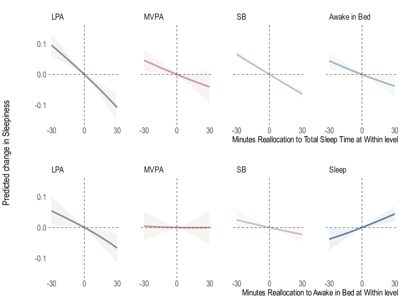
Figure 3: Estimated changes in Sleepiness for Reallocation of 24-hour Sleep-Wake Movement Behaviours.

Notes. LPA = Light Physical Activity, MVPA = Moderate-to-Vigorous Physical Activity, and SB = Sedentary Behavior.

5 Simulation Study

5.1 Aims

In a series of simulation studies, we investigated the performance of the Bayesian compositional MLM and Bayesian compositional substitution MLM in parameter recovery. Our simulation study were based on the real data study, where the objective was to examine the relationship between 24-hour movement behaviour composition and sleepiness.

5.2 Method

5.2.1 Simulation Conditions

We created a range of simulation conditions including different values of the number of clusters ($J$), cluster size ($I$), the number of compositional parts ($D$), and the magnitude of sample variability (assessed by the varying-intercept variance $\sigma^{2}_{u}$ and residual variance $\sigma^{2}_{\varepsilon}$). The values for the number of clusters and cluster sizes were informed by our review of a systematic review and meta-analyses on daily sleep and physical activity [60]. Given the different number of compositional parts used in existing studies, we constructed models with different numbers of possible compositional parts and assessed their performances using different sets of ground truth values. Finally, we examined the influences of sample variability, including varying-intercept variance ($\sigma^{2}_{u}$) and residual variance ($\sigma^{2}_{\varepsilon}$) on the estimation of our models. Table 5 summarises the factors and their levels considered in this simulation study. The combination of these factors resulted in a total of 240 scenarios. For each cell of the simulation design, 2000 replications were generated ($n_{sim}=2000$), resulting in $4[I]\times 4[J]\times 3[D]\times 5[\sigma]\times 2000=$ 480 000 data sets to be analysed.

Table 5: Factors and Their Levels in the Simulation Study.

Factor	Notation	Levels
Number of clusters	J	3, 5, 7, 14
Cluster size	I	30, 50, 360, 1200
Number of compositional parts	D	3, 4, 5
Variance	$\sigma^{2}_{u}$, $\sigma^{2}_{\varepsilon}$	$\sigma^{2}_{u}=1$ and $\sigma^{2}_{\varepsilon}=1$,
		$\sigma^{2}_{u}=1.5$ and $\sigma^{2}_{\varepsilon}=0.5$,
		$\sigma^{2}_{u}=0.5$ and $\sigma^{2}_{\varepsilon}=1.5$,
		$\sigma^{2}_{u}=1$ and $\sigma^{2}_{\varepsilon}=0.5$,
		$\sigma^{2}_{u}=1$ and $\sigma^{2}_{\varepsilon}=1.5$

Notes. $\sigma^{2}_{u}$ = varying-intercept variance, $\sigma^{2}_{\varepsilon}$ = residual variance.

5.2.2 Data Generation

In the following, we described the simulation procedure to generate data sets resembling the data structure used in real data study. The varying-intercept $u_{0j}$ was generated from $\text{Normal}(0,\sigma^{2}_{u})$. The design matrices of the predictors, the between-person $ilr$ ($z^{(b)}$) and within-person $ilr$ ($z^{(w)}$) corresponding to 5-part composition (total sleep time, time in bed awake, MVPA, LPA, and SB) were generated, respectively, as follows:

$$\boldsymbol{z}^{(b)}\sim\text{MVNormal}(\boldsymbol{\mu^{z^{(b)}}},\boldsymbol{\Sigma^{z^{(b)}}})$$

and

$$\boldsymbol{z}^{(w)}\sim\text{MVNormal}(\boldsymbol{\mu^{z^{(w)}}},\boldsymbol{\Sigma^{z^{(w)}}})$$

with values of the means and covariances informed by the data set used in the real data study. Compositional data were then generated by inverse-transforming the 4-dimension $ilr$ coordinates. At this step, when necessary, the 4-part and 3-part compositions were created by collapsing variables. The 4-part composition was obtained by collapsing total sleep time and wake in bed to a single variable named sleep. The 3-part composition was created by collapsing MVPA and LPA to a single variable named physical activity. These compositions were transformed again to $ilr$ coordinates for model estimation.

The outcome vector $\boldsymbol{y}$ was generated from a normal distribution:

$$\boldsymbol{y}\sim\text{Normal}(\gamma_{0}+u_{0j}+\sum_{k=1}^{D-1}\beta_{k}z^{(b)}_{k\boldsymbol{\cdot}j}+\sum_{k=1}^{D-1}\beta_{(k+D-1)}z^{(w)}_{kij},\hskip 5.69046pt\sigma^{2}_{\varepsilon})$$

with the values for the constant parameters set to be close to those found in the real data study.

5.2.3 Estimands

The primary estimands of the simulation study are the parameters of the Bayesian MLM models, including the constant parameter estimates: the intercept ($\gamma_{0}$), the between-person and within-person $ilr$ coordinates ($\beta$s), and the varying parameters: varying-intercept ($\sigma_{u}$) and residual error ($\sigma_{\varepsilon}$). For the Bayesian compositional substitution MLM, estimation of predicted change in outcome at between-level ($\Delta{\hat{y}^{(b)}_{ij}}$) and within-level ($\Delta{\hat{y}^{(w)}_{ij}}$) were evaluated for all possible pairwise substitution between compositional parts, totalling to $2\times D\times(D-1)$ parameters.

5.2.4 Evaluation Criteria

Model performance of 2000 replications across 240 conditions was evaluated using the following criteria.

1. Quality of the MCMC-based sampling procedure of the Bayesian compositional MLM. We considered the proportion of replication that sufficiently converged [[, $\hat{R}<1.05$, ]]vehtari2021 and had no divergent transition. Effective sample size (ESS) was investigated both at the bulk of the distribution (e.g., for the mean or median) and in the tails (e.g., for posterior interval estimates and inferences about extreme quatiles). Any parameters with ESS $>$ 400 indicated sampling inefficiency and required further diagnostics [110].

2. Quality of model performance was evaluated in terms of accuracy in parameter estimates and inference, using three performance measures: bias, coverage, and bias-eliminated coverage [93]. Monte Carlo standard errors were used to calculate 95% confidence interval.

5.2.5 Analysis of Simulated Data

Using package multilevelcoda, each simulated data set was fitted in Bayesian MLM with a varying-intercept to predict next-day sleepiness from the $D$-part behaviour composition, expressed as a total of $2(D-1)$ between- and within-person $ilr$ coordinates. The Bayesian substitution MLM was then conducted, and the model performance in estimating the predicted change in outcome for 30-minute reallocation was evaluated. The simulation study results were summarised using package rsimsum [73] and visualised using package ggplot2 [112]. Reproducible material for this study is available at: https://github.com/florale/multilevelcoda-sim.

5.3 Simulation Results

We found minimal effects of certain simulation conditions on model estimation. Therefore, for brevity, the descriptive statistics of the simulation results of the Bayesian compositional MLM and its associated substitution models were collapsed across 240 conditions and summarised in Table 6.

Table 6: Descriptives Statistics of the Simulation Study.

	Bayesian Compositional MLM	Bayesian Compositional Substitution MLM
Number of divergent transitions	0.01 (0, 134)	-
$\hat{R}$	1.00 (1.00, 1.07)	-
Bulk-ESS	6193.83 (52.06, 27047.59)	-
Tail-ESS	5600.04 (107.91, 9465.94)	-
Bias	0.00 (-0.09, 0.05)	0.00 (-0.03, 0.04)
Coverage	0.95 (0.93, 0.97)	0.95 (0.93, 0.97)
Bias-Eliminated Coverage	0.95 (0.93, 0.97)	0.95 (0.93, 0.97)

Notes. Values are mean and range. MLM = multilevel model.

5.3.1 Quality of Estimation Procedure

Divergences were observed in 1312 replications (0.00%), predominantly with small number of clusters (73.6% $J$: 30), small cluster size (90.5% $I$: 3), and large residual variation (97.6% $\sigma^{2}_{\varepsilon}:1.5$). An additional 17 (0.00%) replications had $\hat{R}>1.05$, demonstrating convergence issues. These replications were excluded for the evaluation of parameter estimates and inference.

In contrast, low bulk ESS were observed as sample size increases with large between-person heterogeneity and small within-person heterogeneity. Particularly, 27 651 replications (0.06%) had bulk $\text{ESS}<400$ for some parameters, predominantly with large number of clusters (51.1% $J$: 1200), large cluster size (70.1% $I$: 14), and small residual variation (95.6% $\sigma^{2}_{\varepsilon}:0.5$). The low ESS values under these conditions represent a technical difficulty posed by the MCMC sampling methods, wherein small variation in the sample (i.e., $\sigma^{2}_{\varepsilon}$) cause the sampler to produce higher within-chain correlation [64]. Additionally, the default non-centered parameterisation [[, i.e., separation of population parameters and hyperparameters in the prior, ]]papaspiliopoulos2007 used in our model estimation procedure can be less efficient for large data sets and strong likelihood (i.e., small sample variability), compared to centered parameterisation [64]. Therefore, we conducted a case study [82] into a replication generated using a 3-part composition, 1200 clusters and cluster size of 14, with large varying intercept variation ($\sigma^{2}_{u}=1.5$) and residual variation ($\sigma^{2}_{\varepsilon}=0.5$), wherein model produced low bulk ESS values for 4 out of 7 parameters. Posterior predictive distributions were checked and two methods to improve the MCMC sampling were tested: centered-parameterisation and increased iterations. We found no evidence of non-convergence (e.g., poor mixing of chains or funnel degeneracy in the posterior). Both reparameterisation or increasing iterations and warm-ups improved ESS, with centered parameterisation showing substantial gain of ESS for the same number of iterations. A sensitivity analysis comparing the model performance with and without the replications with low ESS revealed that ESS did not have an influence on the quality of parameter estimates and inference. Replications with low ESS were, therefore, kept in the subsequent evaluation of model performance.

5.3.2 Quality of Parameter Estimates and Inference

Across the simulated conditions, both Bayesian compositional MLMs and Bayesian compositional substitution MLMs yielded negligible biases in the estimation of all parameters, with a mean of 0.00 and a range from -0.09 to 0.05 and mean of 0.00 and range from -0.03 to 0.04, respectively. Both models had coverage and bias-eliminated coverage close to the nominal value, with means of 0.95 and ranges from 0.93 to 0.97.

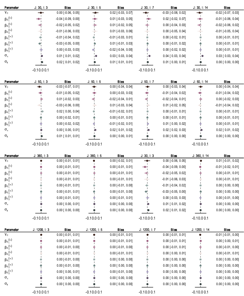
Figure 4: Bias of Bayesian Compositional Multilevel Models with 4-part Composition and Medium Level of Variance

As there was no impact of simulation conditions on the model performance, for brevity, we presented the results for individual parameters estimated using composition with 4 parts ($D$ = 4) and a medium level of modelled variance ($\sigma^{2}_{u}=1$ and $\sigma^{2}_{\varepsilon}=1$) under different conditions of the number of clusters ($J$) and cluster size ($I$). Full results can be accessed via the shiny app by locally running in R using package multilevelcoda. Both models performed well consistently across the number of clusters and cluster size, as demonstrated in Figure 4, 5, 6, and 7.

6 Discussion

EMA and wearable devices to advance clinical and health science have blossomed in the last decade. These methodologies, especially employed in intensive, longitudinal research, have enabled the full day of behaviours and experiences to be captured. In the wake of such data abundance, innovative statistical methods that appropriately address the data properties can enhance psychological studies and lead to new health insights. This paper presented a Bayesian approach to modelling multilevel compositional data, with a focus on both within-person and between-person processes. We described the theories underlying the data and models and illustrated how to perform this method in a real data application. A simulation study confirmed the overall good performance of both Bayesian compositional MLMs and the associated substitution models under different simulation scenarios.

Our empirical results demonstrated the usefulness of the proposed method in examining how day-to-day movement behaviours are associated with other daily experiences using EMA data. We showed that the reallocation of time between movement behaviours was associated with next-day sleepiness, and that this association differed by behaviours involved in the reallocation (e.g., sleep at the expense of MVPA or SB), and whether the effect occurred at the between-person or within-person level. These findings highlight the importance of addressing multilevel and compositional nature of movement behaviours, and any other data with such properties.

Results of the simulation study showed that the quality of estimation procedure was related to sample size and variability. Divergences were observed in a small number of models fitted with small sample sizes and large sample variability, whereas inefficiency of MCMC sampling, indicated by the low ESS, was observed in models fitted with large data sets and small sample variability. The estimation procedure in the simulation study followed a common framework for MCMC sampling [64, 63, 66], and diagnosing and dealing with sampling inefficiency depends on the model of interest and specific applications. Nevertheless, we suggest the following. To eliminate divergences, we recommend using data sets with more than 30 clusters with a cluster size of 3 ($N$ = 90). Studies have already collected data or have sampling limitations may consider adjusting the initial step size and target acceptance rate to assist the sampling departure and trajectories in model estimation [103], such as setting the ?adapt_delta? control parameter to a higher value than the default of 0.80 when fitting model [99]. Scenarios with convergence issues or sampling inefficiency, indicated by low ESS and high $\hat{R}$, may be improved by reparameterisation or increasing the number of warm-up iterations and/or the number of posterior draws. We found that reparameterisation, in particular, yielded the most robust ESS for the same number of iterations.

Bayesian compositional MLMs and Bayesian compositional substitution MLMs both successfully recovered all tested summary statistics, including constant and varying parameters, and residual error. Unbiased estimates and excellent coverage were consistently observed across all conditions of sample sizes, compositional parts, and the magnitude of sample variability. This performance was further not influenced by the efficiency of MCMC sampling. These findings support the advantage of Bayesian over the frequentist approach for MLMs. For frequentist MLMs, a minimum data with 30 clusters with a cluster size of 50 is recommended for models using likelihood estimation methods (either full maximum likelihood or restricted maximum likelihood) to achieve unbiased estimates [90]. MLMs with smaller sample sizes may require Kenward–Roger adjustment [79]. In contrast, we showed that MLMs estimated using Bayesian MCMC sampling can achieve unbiased estimates for data with 30 clusters with a cluster size of 3, and other studies have provided evidence for data with fewer than ten clusters [104, 65]. Another important advantage of our method lies in leveraging Bayesian approach to estimate the substitution model. Using the posterior predictive distributions, the model can directly describe the uncertainty of the estimated quantities (i.e., the predicted changes in outcomes), eliminating the computational burden of relying on resampling techniques, such as bootstrapping, which is typical with frequentist methods.

As with other Bayesian methods, the estimation time required for the models presented in this study is considerable. With more complex models, larger data sets, or when investigating model sensitivity, transforming parameterisation, the amount of time and computational resources can become increasingly substantial. However, we believe that the advantages associated with this method, including accurate and unbiased parameter estimates, straightforward estimation procedure, and minimal convergence issues, outweigh the time and computational cost. Parallelising model fits to multiple cores on a computing cluster can help speed up model estimation process. Our recommended softwares for working with multilevel compositional data, including multilevelcoda, brms, and Stan, all provide several options for fast parallelising Bayesian models.

It is important to note that these models requires complete and non-zero data. Zeros and missing data hamper the analysis of compositional data, as the $ilr$ transformation is essentially based on log ratios. Although dealing with zeros and missing data is outside the scope of this study, previous studies have discussed the zero composition problem [101, 87], provided a comparison of different strategies in dealing with zeros in compositional data [98], and multilevel missing data [86]. Log-ratio Expectation-Maximization [[]]palarea2015 has been recommended for zero imputation as it preserves the relative structure (i.e., ratios) of composition [98]. Imputation strategy based on multivariate MLMs [100, 114] has been shown to produce valid inferences for varying-intercept MLMs with missing data at the lowest level of the multilevel structure [86], such as observations of movement behaviours.

The model of interest in this study was a varying-intercept MLM with a continuous, normally distributed outcome. Other outcome distributions are frequently observed in psychological research, including Bernoulli (binary data, such as depression status), Poisson (count data, such as number of cigarettes smoked per day). Frequentist MLMs with binary outcomes have been shown to be subject to more biased estimation [90]. Three-level data structure (e.g., movement behaviours nested within patients, which in turn are nested within hospitals) are relatively common, and sample sizes can significantly decrease towards the higher level of the data hierarchy. Different prior distributions and their impacts on the expected data were not investigated in our study, due to complexity of the models, the current limited knowledge about behavioural composition and its association with other outcomes. Future work may consider the application of this method and evaluate its performance with other outcome families, more complex random-effect structure (i.e., both varying intercept and varying slopes), more-than-two-level data hierarchy, and steps to build priors and prior consequences on the predictive distribution. Further, recent epidemiological research is increasingly interested in understanding the within-person variability (e.g., changes of behavioural composition at follow-up relative to baseline predicting changes in health outcomes), yet methods are not well established. Our method may be explored in such data sets to extend its impacts to other fields beyond psychology. Lastly, more tutorials detailing step-by-step analyses of example data sets in different areas could help promote wider applications of this innovative method.

7 Conclusion

We introduced an elegant methodology that integrates three statistical frameworks: compositional data analysis, multilevel modelling, and Bayesian inference. The implementation of this method in an open-source R package, multilevelcoda, with a user-friendly setup that only requires the data, model formula and minimal specification of the analysis, speaks to the feasibility of modelling multilevel compositional data in a novel way. As the availability of data with a multilevel compositional structure will grow, we believe this method will be an increasingly important tool to advance psychological research. We hope that our tutorial, evaluations, and recommendations, will motivate researchers to employ this method in their work and discipline to obtain robust answers to scientific questions that otherwise would be inaccessible.

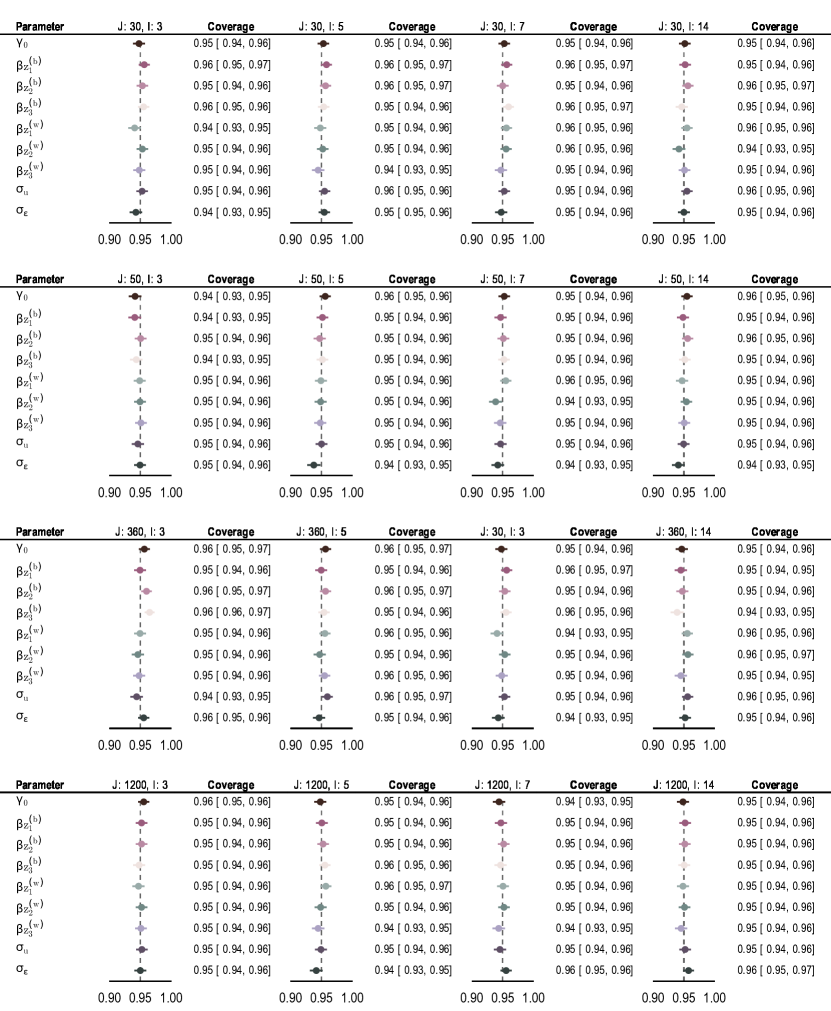
Figure 5: Coverage of Bayesian Compositional Multilevel Models with 4-part Composition and Medium Level of Variance

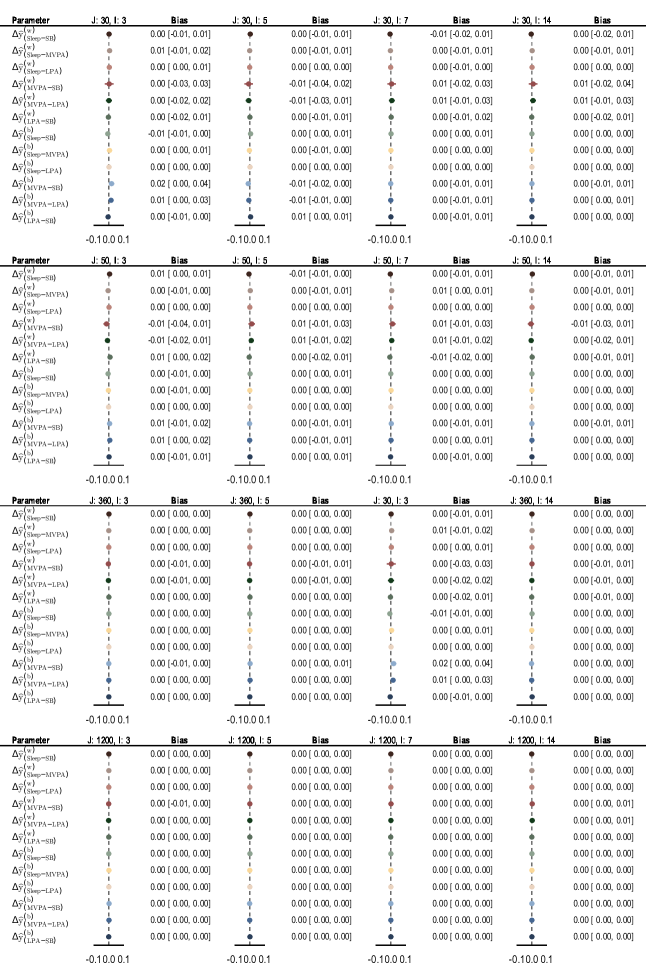
Figure 6: Bias of Bayesian Compositional Substitution Multilevel Models with 4-part Composition and Medium Level of Variance

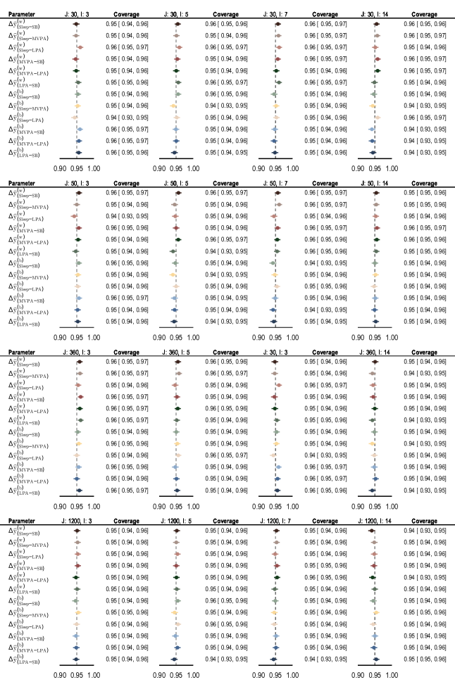
Figure 7: Coverage of Bayesian Compositional Substitution Multilevel Models with 4-part Composition and Medium Level of Variance

References

- [1] John Aitchison “The statistical analysis of compositional data”, Monographs on statistics and applied probability ; [25] London ; New York: ChapmanHall, 1986
- [2] John Aitchison “Principles of compositional data analysis” In Lecture Notes-Monograph Series, 1994, pp. 73–81
- [3] S. Atoui et al. “Daily associations between sleep and physical activity: A systematic review and meta-analysis” In Sleep Medicine Reviews 57, 2021, pp. 101426
- [4] Douglas Bates, Martin Mächler, Ben Bolker and Steve Walker “Fitting linear mixed-effects models using lme4” In Journal of Statistical Software, 2015
- [5] Henrik Bengtsson “A Unifying Framework for Parallel and Distributed Processing in R using Futures” In The R Journal 13.2, 2021, pp. 208–227 DOI: 10.32614/RJ-2021-048
- [6] Michael Betancourt “A conceptual introduction to Hamiltonian Monte Carlo” In arXiv preprint arXiv:1701.02434, 2017
- [7] Michael Betancourt and Mark Girolami “Hamiltonian Monte Carlo for hierarchical models” In Current trends in Bayesian methodology with applications 79.30 CRC Press Boca Raton, FL, 2015, pp. 2–4
- [8] William J Browne and David Draper “A comparison of Bayesian and likelihood-based methods for fitting multilevel models”, 2006
- [9] Paul-Christian Bürkner “brms: An R package for Bayesian multilevel models using Stan” In Journal of Statistical Software 80, 2017, pp. 1–28
- [10] Paul-Christian Bürkner “Prior Definitions for brms Models”, 2024 URL: https://paul-buerkner.github.io/brms/reference/set_prior.html
- [11] Bob Carpenter et al. “Stan: A probabilistic programming language” In Journal of statistical software 76 NIH Public Access, 2017
- [12] Dorothea Dumuid et al. “Compositional data analysis for physical activity, sedentary time and sleep research” In Statistical Methods in Medical Research 27.12 Sage Publications Sage UK: London, England, 2018, pp. 3726–3738
- [13] Dorothea Dumuid et al. “The compositional isotemporal substitution model: a method for estimating changes in a health outcome for reallocation of time between sleep, physical activity and sedentary behaviour” In Statistical Methods in Medical Research 28.3, 2019, pp. 846–857
- [14] Juan José Egozcue and Vera Pawlowsky-Glahn “Groups of parts and their balances in compositional data analysis” In Mathematical Geology 37.7 Springer, 2005, pp. 795–828
- [15] Juan José Egozcue, Vera Pawlowsky-Glahn, Glória Mateu-Figueras and Carles Barcelo-Vidal “Isometric logratio transformations for compositional data analysis” In Mathematical Geology 35.3, 2003, pp. 279–300
- [16] A. Gasparini “rsimsum: Summarise results from Monte Carlo simulation studies” In Journal of Open Source Software 3, 2018, pp. 739 DOI: 10.21105/joss.00739
- [17] A. Gelman et al. “Bayesian data analysis”, CBMS-NSF Regional Conference Series CRC press, 2013
- [18] Jozo Grgic et al. “Health outcomes associated with reallocations of time between sleep, sedentary behaviour, and physical activity: a systematic scoping review of isotemporal substitution studies” In International Journal of Behavioral Nutrition and Physical Activity 15.1 BioMed Central, 2018, pp. 1–68
- [19] Claire Groves et al. “Optimal combinations of 24-hour movement behaviors for mental health across the lifespan: A systematic review” PsyArXiv, 2023
- [20] Kimberly R Hartson et al. “Use of Electronic Ecological Momentary Assessment Methodologies in Physical Activity, Sedentary Behavior, and Sleep Research in Young Adults: Systematic Review” In Journal of Medical Internet Research 25 JMIR Publications Toronto, Canada, 2023, pp. e46783
- [21] Ian Janssen et al. “A systematic review of compositional data analysis studies examining associations between sleep, sedentary behaviour, and physical activity with health outcomes in adults” In Applied physiology, nutrition, and metabolism 45.10 NRC Research Press 1840 Woodward Drive, Suite 1, Ottawa, ON K2C 0P7, 2020, pp. S248–S257
- [22] Michael G Kenward and James H Roger “Small sample inference for fixed effects from restricted maximum likelihood” In Biometrics JSTOR, 1997, pp. 983–997
- [23] J. Kruschke “Doing Bayesian data analysis: A tutorial with R, JAGS, and Stan”, 2014
- [24] F. Le et al. “The associations between daily activities and affect a compositional isotemporal substitution analysis” In International Journal of Behavioral Medicine 29, 2022, pp. 456–468 DOI: https://doi.org/10.1007/s12529-021-10031-z
- [25] Flora Le “Improving MCMC Sampling for Bayesian Compositional Multilevel Models”, 2024 URL: https://florale.github.io/multilevelcoda/articles/E-simmodel-diag.html
- [26] Flora Le and Joshua F Wiley “multilevelcoda: Estimate Bayesian Multilevel Models for Compositional Data” R package version 1.2.1, 2023 URL: https://CRAN.R-project.org/package=multilevelcoda
- [27] Flora Le, Dorothea Dumuid, Tyman E. Stanford and Joshua F. Wiley “multilevelcoda: An R package for Bayesian Multilevel Compositional Data Analysis [Manuscript submitted for publication]”, 2024
- [28] Roy Levy and Daniel McNeish “Perspectives on Bayesian inference and their implications for data analysis.” In Psychological Methods 28.3 American Psychological Association, 2023, pp. 719
- [29] Oliver Lüdtke, Alexander Robitzsch and Simon Grund “Multiple imputation of missing data in multilevel designs: A comparison of different strategies.” In Psychological Methods 22.1 American Psychological Association, 2017, pp. 141
- [30] Josep A Martín-Fernández, Carles Barceló-Vidal and Vera Pawlowsky-Glahn “Dealing with zeros and missing values in compositional data sets using nonparametric imputation” In Mathematical Geology 35 Springer, 2003, pp. 253–278
- [31] Gloria Mateu-Figueras, Vera Pawlowsky-Glahn and Juan José Egozcue “The principle of working on coordinates” In Compositional data analysis Wiley Online Library, 2011, pp. 29–42
- [32] Richard McElreath “Statistical rethinking: A Bayesian course with examples in R and Stan” ChapmanHall/CRC, 2018
- [33] Daniel M McNeish and Laura M Stapleton “The effect of small sample size on two-level model estimates: A review and illustration” In Educational Psychology Review 28 Springer, 2016, pp. 295–314
- [34] Aaron Miatke et al. “The association between reallocations of time and health using compositional data analysis: a systematic scoping review with an interactive data exploration interface” In International Journal of Behavioral Nutrition and Physical Activity 20.1 Springer, 2023, pp. 127
- [35] Jairo H Migueles et al. “GGIR: A Research Community-Driven Open Source R Package for Generating Physical Activity and Sleep Outcomes From Multi-Day Raw Accelerometer Data” In Journal for the Measurement of Physical Behavior 2.3, 2019 DOI: 10.1123/jmpb.2018-0063
- [36] Tim P Morris, Ian R White and Michael J Crowther “Using simulation studies to evaluate statistical methods” In Statistics in medicine 38.11 Wiley Online Library, 2019, pp. 2074–2102
- [37] Javier Palarea-Albaladejo and Josep Antoni Martín-Fernández “zCompositions—R package for multivariate imputation of left-censored data under a compositional approach” In Chemometrics and Intelligent Laboratory Systems 143 Elsevier, 2015, pp. 85–96
- [38] Omiros Papaspiliopoulos, Gareth O Roberts and Martin Sköld “A general framework for the parametrization of hierarchical models” In Statistical Science JSTOR, 2007, pp. 59–73
- [39] Vera Pawlowsky-Glahn and Antonella Buccianti “Compositional data analysis” Wiley Online Library, 2011
- [40] R Core Team “R: A Language and Environment for Statistical Computing” Version 4.2.1, 2022 R Foundation for Statistical Computing URL: https://www.R-project.org/
- [41] Charlotte Lund Rasmussen et al. “Zero problems with compositional data of physical behaviours: a comparison of three zero replacement methods” In International Journal of Behavioral Nutrition and Physical Activity 17.1 BioMed Central, 2020, pp. 1–10
- [42] Daniel J Schad, Michael Betancourt and Shravan Vasishth “Toward a principled Bayesian workflow in cognitive science.” In Psychological Methods 26.1 American Psychological Association, 2021, pp. 103
- [43] Joseph L Schafer and Recai M Yucel “Computational strategies for multivariate linear mixed-effects models with missing values” In Journal of computational and Graphical Statistics 11.2 Taylor & Francis, 2002, pp. 437–457
- [44] Michael Smithson and Stephen B Broomell “Compositional data analysis tutorial.” In Psychological Methods American Psychological Association, 2022
- [45] Stan Development Team “cmdstanr: the R interface to CmdStan” Version 2.30.1, 2022 URL: https://mc-stan.org/cmdstanr/
- [46] Stan Development Team “Stan Reference Manual”, 2023 URL: http://mc-stan.org/
- [47] Daniel Stegmueller “How many countries for multilevel modelling? A comparison of frequentist and Bayesian approaches” In American journal of political science 57.3 Wiley Online Library, 2013, pp. 748–761
- [48] K Gerald Van den Boogaart and Raimon Tolosana-Delgado “Analyzing compositional data with R” Springer, 2013
- [49] Vincent T van Hees et al. “Autocalibration of accelerometer data for free-living physical activity assessment using local gravity and temperature: an evaluation on four continents” In Journal of Applied Physiology 117.7, 2014, pp. 738–744 URL: https://doi.org/10.1152/japplphysiol.00421.2014
- [50] Vincent T van Hees et al. “A Novel, Open Access Method to Assess Sleep Duration Using a Wrist-Worn Accelerometer” In PLoS One 10.11, 2015 DOI: 10.1371/journal.pone.0142533
- [51] Vincent T van Hees et al. “Estimating sleep parameters using an accelerometer without sleep diary” In Scientific Reports 8.1, 2018 DOI: 10.1038/s41598-018-31266-z
- [52] Vincent T van Hees et al. “GGIR: Raw Accelerometer Data Analysis” R package version 2.10-1, 2023 DOI: 10.5281/zenodo.1051064
- [53] Aki Vehtari et al. “Rank-normalization, folding, and localization: An improved R̂ for assessing convergence of MCMC (with discussion)” In Bayesian analysis 16.2 International Society for Bayesian Analysis, 2021, pp. 667–718
- [54] Eric-Jan Wagenmakers, Richard D Morey and Michael D Lee “Bayesian benefits for the pragmatic researcher” In Current Directions in Psychological Science 25.3 Sage Publications Sage CA: Los Angeles, CA, 2016, pp. 169–176
- [55] Hadley Wickham “ggplot2: Elegant Graphics for Data Analysis” Version 3.4.0 Springer-Verlag New York, 2016 URL: https://ggplot2.tidyverse.org
- [56] Yang Yap et al. “Bi-directional relations between stress and self-reported and actigraphy-assessed sleep: a daily intensive longitudinal study” In Sleep 43.3 Oxford University Press US, 2020, pp. zsz250
- [57] JH Zhao and JL Schafer “pan: Multiple imputation for multivariate panel or clustered data” R package version 1.9, 2023 URL: https://CRAN.R-project.org/package=pan
- [58] John Aitchison “The statistical analysis of compositional data”, Monographs on statistics and applied probability ; [25] London ; New York: ChapmanHall, 1986
- [59] John Aitchison “Principles of compositional data analysis” In Lecture Notes-Monograph Series, 1994, pp. 73–81
- [60] S. Atoui et al. “Daily associations between sleep and physical activity: A systematic review and meta-analysis” In Sleep Medicine Reviews 57, 2021, pp. 101426
- [61] Douglas Bates, Martin Mächler, Ben Bolker and Steve Walker “Fitting linear mixed-effects models using lme4” In Journal of Statistical Software, 2015
- [62] Henrik Bengtsson “A Unifying Framework for Parallel and Distributed Processing in R using Futures” In The R Journal 13.2, 2021, pp. 208–227 DOI: 10.32614/RJ-2021-048
- [63] Michael Betancourt “A conceptual introduction to Hamiltonian Monte Carlo” In arXiv preprint arXiv:1701.02434, 2017
- [64] Michael Betancourt and Mark Girolami “Hamiltonian Monte Carlo for hierarchical models” In Current trends in Bayesian methodology with applications 79.30 CRC Press Boca Raton, FL, 2015, pp. 2–4
- [65] William J Browne and David Draper “A comparison of Bayesian and likelihood-based methods for fitting multilevel models”, 2006
- [66] Paul-Christian Bürkner “brms: An R package for Bayesian multilevel models using Stan” In Journal of Statistical Software 80, 2017, pp. 1–28
- [67] Paul-Christian Bürkner “Prior Definitions for brms Models”, 2024 URL: https://paul-buerkner.github.io/brms/reference/set_prior.html
- [68] Bob Carpenter et al. “Stan: A probabilistic programming language” In Journal of statistical software 76 NIH Public Access, 2017
- [69] Dorothea Dumuid et al. “The compositional isotemporal substitution model: a method for estimating changes in a health outcome for reallocation of time between sleep, physical activity and sedentary behaviour” In Statistical Methods in Medical Research 28.3, 2019, pp. 846–857
- [70] Dorothea Dumuid et al. “Compositional data analysis for physical activity, sedentary time and sleep research” In Statistical Methods in Medical Research 27.12 Sage Publications Sage UK: London, England, 2018, pp. 3726–3738
- [71] Juan José Egozcue and Vera Pawlowsky-Glahn “Groups of parts and their balances in compositional data analysis” In Mathematical Geology 37.7 Springer, 2005, pp. 795–828
- [72] Juan José Egozcue, Vera Pawlowsky-Glahn, Glória Mateu-Figueras and Carles Barcelo-Vidal “Isometric logratio transformations for compositional data analysis” In Mathematical Geology 35.3, 2003, pp. 279–300
- [73] A. Gasparini “rsimsum: Summarise results from Monte Carlo simulation studies” In Journal of Open Source Software 3, 2018, pp. 739 DOI: 10.21105/joss.00739
- [74] A. Gelman et al. “Bayesian data analysis”, CBMS-NSF Regional Conference Series CRC press, 2013
- [75] Jozo Grgic et al. “Health outcomes associated with reallocations of time between sleep, sedentary behaviour, and physical activity: a systematic scoping review of isotemporal substitution studies” In International Journal of Behavioral Nutrition and Physical Activity 15.1 BioMed Central, 2018, pp. 1–68
- [76] Claire Groves et al. “Optimal combinations of 24-hour movement behaviors for mental health across the lifespan: A systematic review” PsyArXiv, 2023
- [77] Kimberly R Hartson et al. “Use of Electronic Ecological Momentary Assessment Methodologies in Physical Activity, Sedentary Behavior, and Sleep Research in Young Adults: Systematic Review” In Journal of Medical Internet Research 25 JMIR Publications Toronto, Canada, 2023, pp. e46783
- [78] Ian Janssen et al. “A systematic review of compositional data analysis studies examining associations between sleep, sedentary behaviour, and physical activity with health outcomes in adults” In Applied physiology, nutrition, and metabolism 45.10 NRC Research Press 1840 Woodward Drive, Suite 1, Ottawa, ON K2C 0P7, 2020, pp. S248–S257
- [79] Michael G Kenward and James H Roger “Small sample inference for fixed effects from restricted maximum likelihood” In Biometrics JSTOR, 1997, pp. 983–997
- [80] J. Kruschke “Doing Bayesian data analysis: A tutorial with R, JAGS, and Stan”, 2014
- [81] F. Le et al. “The associations between daily activities and affect a compositional isotemporal substitution analysis” In International Journal of Behavioral Medicine 29, 2022, pp. 456–468 DOI: https://doi.org/10.1007/s12529-021-10031-z
- [82] Flora Le “Improving MCMC Sampling for Bayesian Compositional Multilevel Models”, 2024 URL: https://florale.github.io/multilevelcoda/articles/E-simmodel-diag.html
- [83] Flora Le, Dorothea Dumuid, Tyman E. Stanford and Joshua F. Wiley “multilevelcoda: An R package for Bayesian Multilevel Compositional Data Analysis [Manuscript submitted for publication]”, 2024
- [84] Flora Le and Joshua F Wiley “multilevelcoda: Estimate Bayesian Multilevel Models for Compositional Data” R package version 1.2.1, 2023 URL: https://CRAN.R-project.org/package=multilevelcoda
- [85] Roy Levy and Daniel McNeish “Perspectives on Bayesian inference and their implications for data analysis.” In Psychological Methods 28.3 American Psychological Association, 2023, pp. 719
- [86] Oliver Lüdtke, Alexander Robitzsch and Simon Grund “Multiple imputation of missing data in multilevel designs: A comparison of different strategies.” In Psychological Methods 22.1 American Psychological Association, 2017, pp. 141
- [87] Josep A Martín-Fernández, Carles Barceló-Vidal and Vera Pawlowsky-Glahn “Dealing with zeros and missing values in compositional data sets using nonparametric imputation” In Mathematical Geology 35 Springer, 2003, pp. 253–278
- [88] Gloria Mateu-Figueras, Vera Pawlowsky-Glahn and Juan José Egozcue “The principle of working on coordinates” In Compositional data analysis Wiley Online Library, 2011, pp. 29–42
- [89] Richard McElreath “Statistical rethinking: A Bayesian course with examples in R and Stan” ChapmanHall/CRC, 2018
- [90] Daniel M McNeish and Laura M Stapleton “The effect of small sample size on two-level model estimates: A review and illustration” In Educational Psychology Review 28 Springer, 2016, pp. 295–314
- [91] Aaron Miatke et al. “The association between reallocations of time and health using compositional data analysis: a systematic scoping review with an interactive data exploration interface” In International Journal of Behavioral Nutrition and Physical Activity 20.1 Springer, 2023, pp. 127
- [92] Jairo H Migueles et al. “GGIR: A Research Community-Driven Open Source R Package for Generating Physical Activity and Sleep Outcomes From Multi-Day Raw Accelerometer Data” In Journal for the Measurement of Physical Behavior 2.3, 2019 DOI: 10.1123/jmpb.2018-0063
- [93] Tim P Morris, Ian R White and Michael J Crowther “Using simulation studies to evaluate statistical methods” In Statistics in medicine 38.11 Wiley Online Library, 2019, pp. 2074–2102
- [94] Javier Palarea-Albaladejo and Josep Antoni Martín-Fernández “zCompositions—R package for multivariate imputation of left-censored data under a compositional approach” In Chemometrics and Intelligent Laboratory Systems 143 Elsevier, 2015, pp. 85–96
- [95] Omiros Papaspiliopoulos, Gareth O Roberts and Martin Sköld “A general framework for the parametrization of hierarchical models” In Statistical Science JSTOR, 2007, pp. 59–73
- [96] Vera Pawlowsky-Glahn and Antonella Buccianti “Compositional data analysis” Wiley Online Library, 2011
- [97] R Core Team “R: A Language and Environment for Statistical Computing” Version 4.2.1, 2022 R Foundation for Statistical Computing URL: https://www.R-project.org/
- [98] Charlotte Lund Rasmussen et al. “Zero problems with compositional data of physical behaviours: a comparison of three zero replacement methods” In International Journal of Behavioral Nutrition and Physical Activity 17.1 BioMed Central, 2020, pp. 1–10
- [99] Daniel J Schad, Michael Betancourt and Shravan Vasishth “Toward a principled Bayesian workflow in cognitive science.” In Psychological Methods 26.1 American Psychological Association, 2021, pp. 103
- [100] Joseph L Schafer and Recai M Yucel “Computational strategies for multivariate linear mixed-effects models with missing values” In Journal of computational and Graphical Statistics 11.2 Taylor & Francis, 2002, pp. 437–457
- [101] Michael Smithson and Stephen B Broomell “Compositional data analysis tutorial.” In Psychological Methods American Psychological Association, 2022
- [102] Stan Development Team “cmdstanr: the R interface to CmdStan” Version 2.30.1, 2022 URL: https://mc-stan.org/cmdstanr/
- [103] Stan Development Team “Stan Reference Manual”, 2023 URL: http://mc-stan.org/
- [104] Daniel Stegmueller “How many countries for multilevel modelling? A comparison of frequentist and Bayesian approaches” In American journal of political science 57.3 Wiley Online Library, 2013, pp. 748–761
- [105] K Gerald Van den Boogaart and Raimon Tolosana-Delgado “Analyzing compositional data with R” Springer, 2013
- [106] Vincent T van Hees et al. “Autocalibration of accelerometer data for free-living physical activity assessment using local gravity and temperature: an evaluation on four continents” In Journal of Applied Physiology 117.7, 2014, pp. 738–744 URL: https://doi.org/10.1152/japplphysiol.00421.2014
- [107] Vincent T van Hees et al. “GGIR: Raw Accelerometer Data Analysis” R package version 2.10-1, 2023 DOI: 10.5281/zenodo.1051064
- [108] Vincent T van Hees et al. “A Novel, Open Access Method to Assess Sleep Duration Using a Wrist-Worn Accelerometer” In PLoS One 10.11, 2015 DOI: 10.1371/journal.pone.0142533
- [109] Vincent T van Hees et al. “Estimating sleep parameters using an accelerometer without sleep diary” In Scientific Reports 8.1, 2018 DOI: 10.1038/s41598-018-31266-z
- [110] Aki Vehtari et al. “Rank-normalization, folding, and localization: An improved R̂ for assessing convergence of MCMC (with discussion)” In Bayesian analysis 16.2 International Society for Bayesian Analysis, 2021, pp. 667–718
- [111] Eric-Jan Wagenmakers, Richard D Morey and Michael D Lee “Bayesian benefits for the pragmatic researcher” In Current Directions in Psychological Science 25.3 Sage Publications Sage CA: Los Angeles, CA, 2016, pp. 169–176
- [112] Hadley Wickham “ggplot2: Elegant Graphics for Data Analysis” Version 3.4.0 Springer-Verlag New York, 2016 URL: https://ggplot2.tidyverse.org
- [113] Yang Yap et al. “Bi-directional relations between stress and self-reported and actigraphy-assessed sleep: a daily intensive longitudinal study” In Sleep 43.3 Oxford University Press US, 2020, pp. zsz250
- [114] JH Zhao and JL Schafer “pan: Multiple imputation for multivariate panel or clustered data” R package version 1.9, 2023 URL: https://CRAN.R-project.org/package=pan