A hydrodynamic approach to reproduce multiple spinning vortices in horizontally rotating three-dimensional liquid helium-4

Abstract

This paper reports a three-dimensional (3D) simulation of a rotating liquid, helium-4, using a two-fluid model with spin-angular momentum conservation. Our model was derived from the particle approximation of an inviscid fluid with residual viscosity. Despite the fully classical mechanical picture, the resulting system equations were consistent with those of the conventional two-fluid model. We consider bulk liquid helium-4 to be an inviscid fluid, assuming that the viscous fluid component remains at finite temperatures. As the temperature decreased, the amount of the viscous fluid component decreased, ultimately becoming a fully inviscid fluid at absolute zero. Weak compressibility is assumed to express the volume change because some helium atoms do not render fluid owing to BECs or change states because of local thermal excitation. One can solve the governing equations for an incompressible fluid using explicit SPH (smoothed particle hydrodynamics), simultaneously reproducing density fluctuations and describing the fluid in a many-particle system. We assume the following fluid-particle duality: a hydrodynamic interfacial tension between the inviscid and viscous components or a local interaction force between two types of fluid particles. The former can be induced in the horizontal direction when non-negligible non-uniformity of the particles occurs during forced two-dimensional rotation, and the latter is non-negligible when the former is negligible. We performed a large-scale simulation of 3D liquid helium forced to rotate horizontally using 32 GPUs. Compared with the low-resolution calculation using 2.4 million particles, the high-resolution calculation using 19.6 million particles showed spinning vortices close to those of the theoretical solution. We obtained a promising venue to establish a practical simulation method for bulk liquid helium-4.

1 Introduction

Liquid helium-4 has a long history of use in various engineering and scientific fields. In particular, it has been used as a refrigerant for superconducting magnets in magnetic resonance imaging (MRI) and has been studied for cooling superconducting motors for rapid long-distance mobility. In general, two types of cooling methods are used in superconducting systems. The first is low-temperature superconductivity, an example of which is a niobium-titanium alloy cooled by liquid helium to near absolute zero (0 to about 4.2 K: Kelvin) [1, 2]. The second type is high-temperature superconductivity, in which a special metallic compound is cooled to a relatively high temperature of approximately 100 K using liquid nitrogen to achieve a superconducting state. Low-temperature superconductivity has the advantage of high critical current density. However, according to quantum mechanics, liquid helium loses its viscosity when cooled to near absolute zero owing to Bose-Einstein condensation to the ground state of energy, and this quantum effect often causes a severe leakage phenomenon (super leakage). In addition, it only enters the solid state under high pressure and thus must be used as a coolant in the liquid state. In other words, the stable control of liquid helium in a cooling system is very difficult in low-temperature superconductivity. Stable cooling with liquid nitrogen enables high-temperature superconductivity. However, the critical current density is small, and the current that can maintain the superconducting state is weak; therefore, it cannot withstand practical use. Thus, neither cooling method is one step away from practical application owing to the trade-off between the difficulty of cooling and the critical current density; this is a factor that hinders the full industrialization of superconducting motors.

If it were possible to perform large-scale simulations on recent supercomputers to reproduce the dynamics of bulk liquid helium-4, the following would be expected. First, it would be possible to precisely predict and control the occurrence of super leakage due to quantum effects in the dynamics of superfluid helium; this will enable the stable control and safety of superfluid helium in large-scale cooling systems at a low development cost. Consequently, the practicality of superfluid helium as a cold agent in low-temperature superconductivity is expected to be dramatically enhanced. In addition, it is expected to significantly reduce the consumption of liquid helium during cryogenic experiments. It has been reported that the carbon dioxide emitted from the production and transportation of liquid helium can reach 587 kg-CO2/l [3]. If the dynamics of bulk liquid helium can be simulated by large-scale simulation technology using a supercomputer, the number of experiments using liquid helium can be reduced by half, leading to a reduction in carbon dioxide emissions.

This study developed a new simulation technique that can reproduce the three-dimensional (3D) fluid behavior of superfluid helium-4 in a cryogenic cooling system on a real scale. As of yet, most simulation methods for liquid helium have been based on quantum mechanical scale simulations that aim to elucidate the principles, and there has been little progress in the development of numerical methods for so-called “bulk state” quantum fluids. Next, we discuss the properties of helium-4 at cryogenic temperatures. In principle, the mechanism of liquid helium can be described using quantum mechanics, which is the governing law of the nanoscale. Helium-4 is a so-called Bose particle consisting of two neutrons and two protons. Bose particles have quantized angular momentum times an integer. In this paper, “helium” indicates helium-4 unless otherwise noted. Liquid helium-4 can be described as a many-particle interaction system of Bose particles. However, unlike ordinary materials that solidify in low-temperature regions, helium-4 exists as a liquid even near absolute zero. Therefore, liquid helium has the strange property of locally obeying quantum mechanical laws while behaving as a fluid, a continuum, as a whole. In a many-particle interacting system of Bosonic particles below a critical temperature near absolute zero, helium atoms in a particular region undergo Bose-Einstein condensation (BEC), in which they fall into the ground energy state; this minimizes the interaction between helium atoms. (Helium is a monatomic molecule, but we use the term “molecular viscosity” in accordance with the chemical engineering doctrine [4, 5]). In other words, liquid helium-4 loses its viscosity at cryogenic temperatures below the critical temperature, that is, it becomes an inviscid fluid.

The fact that liquid helium becomes an inviscid fluid causes peculiar fluid phenomena, such as slipping through the microstructure of the porous medium (gypsum), which is not observed when liquid helium is composed only of viscous normal flow components, and film flow caused by the viscosity between the wall surface and helium atoms being larger than the viscosity between helium atoms. These phenomena are often described as “macroscopic quantum phenomena” because the disappearance of microscopic interactions, i.e., of molecular viscosity, affects the macroscopic fluid behavior of bulk liquid helium. In addition to the phenomena that can be observed with the naked eye, vortex lattice phenomena observed on the nanometer scale in rotating liquid helium are also macroscopic quantum phenomena that can be observed between the hydrodynamic and quantum mechanical regimes. To the best of our knowledge, no study has successfully simulated the vortex lattice phenomena of rotating 3D liquid helium-4 observed in the boundary regime between these two different dynamical regimes using a method based on classical fluid mechanics.

It is widely recognized that the macroscopic behavior of liquid helium-4 can be phenomenologically described by the two-fluid model proposed by L. Landau, which consists of an inviscid fluid and incompressible Navier-Stokes equations. However, it should be noted that this assumption has only been verified by the issue of countercurrent flow, in which shear viscosity is dominant. Macroscopic quantum phenomena observed in the rotation problem, such as vortex lattices, have yet to be numerically reproduced using two-fluid models. The authors hypothesized that the main reason for this is that the ordinary two-fluid model does not reflect the quantization of the spin angular momentum of individual helium-4 atoms when liquid helium-4 is considered as a microscopic many-particle interacting system. As stated previously, the spin angular momentum of the Bose particles was quantized. If fluid particles, which are virtual constituent particles in fluid mechanics, can be interpreted as a type of coarse-grained model of such microscopic particles, then the angular momentum related to the spin of the constituent atoms should also be conserved in the fluid particles.

Considering this hypothesis, the author recently developed a two-fluid model with spin-angular momentum conservation [6, 7, 8]. The following overview provides a general introduction to this subject. The Navier-Stokes equation with conservation of rotational angular momentum around the axes of fluid particles was originally derived from the constitutive law of continuum mechanics by D. Condiff in 1964 [9]. Half a century later, K. Müller [10] developed a particle approximation of the Navier-Stokes equation with spin-angular momentum conservation using smoothed particle hydrodynamics (SPH) [11, 12] for mesoscale thermal flow. Considering these studies, the author adopted the Navier-Stokes equations with spin-angular momentum conservation for normal fluids and employed SPH to discretize the equation systems using particles. In other words, we describe liquid helium-4 as a system of numerous particle interactions composed of two distinct types of classical fluid particles that maintain their rotational angular velocity around their axes under the assumption of rigid body rotations; this is referred to as a two-fluid model with spin-angular momentum conservation. More importantly, our two-fluid model differs from conventional models in terms of the physical picture. The conventional two-fluid model was derived by combining the nonlinear $\rm Schr\ddot{o}dinger$ equation for bosons with the thermodynamic Gibbs-Duhem equation. Conversely, our model considers the bulk of liquid helium-4 at low temperatures as an inviscid fluid following continuum mechanics, which contains residual viscosity at finite temperatures. In summary, the proposed model is based on a two-phase flow. Despite the fully classical mechanical picture, the resulting system equations were consistent with an ordinary model (see Eqs. (1) and (2)). In particular, we consider the bulk liquid helium-4 to be an inviscid fluid, assuming that the viscous fluid component remains at finite temperatures. As the temperature decreased, the amount of the viscous fluid component decreased, ultimately becoming a fully inviscid fluid at absolute zero. From the Lagrangian perspective, our two-fluid model is a mixture of fluid particles from inviscid and viscous fluid components. Both fluid particles are classical fluid particles; they are virtual particles. Thus, our model is based on the mixing of two classical fluids and is similar to a two-phase flow model. However, as described below, we allow for a certain “nature of particles” of both components as a correction. In this context, the physical picture in which the viscous fluid component remains bead-like in an inviscid fluid is a more accurate representation of the system than a two-phase flow model. This is also close to the image of a “nanofluid,” or nanoparticle dispersion system. Details of this technique are described in Refs. [6, 7, 8]. This will be outlined later in this paper. In our previous simulations of rotating two-dimensional (2D) liquid helium-4, we observed the formation of multiple spinning vortices that occurred independently of the overall fluid motion. After incorporating the vortex dynamics model into our model, we found that multiple spinning vortices formed a lattice with a regular arrangement. The number of vortices generated is determined by the strength of the rotational angular velocity. For appropriate values, the number of vortices agrees well with the theoretical solution of the number of vortices calculated from Feynman’s law. It is also noteworthy that the spinning of each vortex moves independently without affecting the behavior of the entire fluid. In other words, the vortices do not dissipate. In a quantum vortex, the vortices do not dissipate because of the circulation quantization. This important property can also be reproduced. Consequently, the vortex lattice phenomenon in the rotating 2D liquid helium-4 was simulated by solving the two-fluid model with spin angular momentum conservation.

This study presents the observation of independently spinning three-dimensional vortices in 3D liquid helium-4 in a cylindrical container rotated horizontally using the aforementioned two-fluid model with spin angular momentum conservation. In the context of quantum hydrodynamics, the dynamics of the connections or reconnections of 3D vortex lines differ from those in classical dynamics owing to quantized circulations. Consequently, the topological variations in the 2D vortex lines are not analogous to those in the 3D vortex lines. For example, two vortex lines can occupy skew positions relative to one another in space, resulting in only two distinct patterns of reconnection between vortex line-line interactions and vortex line-wall interactions. In addition, from the perspective of polyhedral geometry, angle management in 3D space requires the use of quaternions to circumvent singularities. The dynamics of quantum fluids in 3D space are complex and, in fact, not an extension of those in 2D space; the cross-section of a vortex line in real cases is projected onto a plate in 2D space. The geometric complexity in 3D space indicates that computational methods in 3D space must be verified and validated independently of the results in 2D cases. Therefore, it is unclear whether the authors’ method, which was effective in solving the 2D rotating problem, can numerically reproduce the dynamics of 3D liquid helium-4. For clarity, we excluded the vortex dynamics model effective for 2D liquid helium-4 designed in our previous studies [7] when applying our two-fluid model to 3D cases. We only focused on discretizing our two-fluid model in 3D space. Artificial manipulations such as those proposed by K. W. Schwarz [13, 14] were not considered in this study. Nevertheless, we succeeded in reproducing several 3D vortices spinning in the horizontal direction during the horizontal rotation of liquid helium-4. The scientific significance of our numerical results is discussed in Section 4. The remainder of this paper is organized as follows. In Section 2, we provide an overview of the proposed two-fluid model and the 3D calculations on a parallel computing platform. In Section 3, we present the numerical results of our simulations of 3D liquid helium-4 rotating horizontally. In Section 4, we discuss the scientific significance of the results obtained. Finally, Section 5 concludes the study.

2 Methods

2.1 The two-fluid model with spin angular momentum conservation

Our two-fluid model differs from the ordinary two-fluid model in its derivation and interpretation of the equation. Here, the ordinary two-fluid model is derived from the following microscopic relations. More specifically, the Navier-Stokes equation for an incompressible fluid with a temperature gradient term was derived by solving the Gross-Pitaevskii equation, which is a nonlinear Schrödinger equation, and the Gibbs-Duhem thermodynamic relation in conjunction. This equation describes the dynamics of the superfluid component. In short, the usual two-fluid model is obtained by making “macro-corrections” to the microscopic relational equations. The governing equation for the normal flow component was obtained by subtracting the equation for the superfluid component from the equation of motion for an incompressible fluid. In a domain where quantum mechanics is dominant, the superfluid and normal flow components exist independently, and the two components together are considered to conserve mass and momentum (although entropy is said to be carried only by the normal flow component). This microscopic picture was proposed by Tiza and Landau [15, 16] and was subsequently verified by countercurrent flow experiments. Originally, the two components were considered completely independent; however, experiments have shown that when the heat input is large, the two components exert a mutual frictional force proportional to the velocity difference between them  [17].

By contrast, the concept and derivation of our two-fluid model are quite the opposite. Notably, we obtain a system of two equations of the same form as in the two-fluid model described above by making particle corrections to the fluid equations, which are macroscopic expressions of relations in the domain dominated by continuum mechanics. The details are as follows. First, bulk liquid helium at cryogenic temperatures is considered an inviscid fluid. Subsequently, we assume that the viscous fluid component remains at a finite temperature. The amount of the viscous fluid component decreased as the temperature decreased; at absolute zero, it became a completely inviscid fluid. In other words, our two-fluid model assumes the mixing of the fluid components of inviscid and viscous fluids. Thus, the “fluid particles” in our model are virtual particles in classical fluid mechanics. Liquid helium, on the other hand, is usually considered an incompressible fluid. However, helium atoms are known to cause Bose-Einstein condensations (BECs) when cooled to the critical temperature (interestingly, although liquid helium is commonly described as a multiparticle system of Bose particles, only 13 % of it actually causes BEC even at absolute zero [18]). In any case, the condensate components were no longer fluid. These state changes to and from the condensates are described using quantum statistical mechanics. In other words, from a microscopic viewpoint, the composition ratio of the condensate component to the normal fluid component fluctuates around the average value. Therefore, it can be assumed that the fluid volume fluctuated around the mean value of the equilibrium state. From a macroscopic perspective, the bulk of liquid helium-4 was compressed by a few percent to approximately 13% in the low-temperature regime, and the volume changed around the average. Accordingly, this physical picture is compatible with the fluid computational model of the explicit SPH method. The explicit SPH method uses a finite-particle approximation of the incompressible Navier-Stokes equations. However, instead of implicitly solving the Poisson equation for pressure, as is typically done for incompressible fluids, this method solves the equation of state of a fluid, for example, the Tait equation of state [19]. This approach essentially reproduces density fluctuations [20, 21, 22]. An important point is that we assumed weak compressibility for liquid helium. The ability to solve the Navier-Stokes equations for an incompressible fluid while reproducing its weakly compressible properties is a feature of explicit SPH. In summary, in our two-fluid model, liquid helium is considered an inviscid fluid, and it is assumed that the viscous fluid component remains a function of temperature. In other words, it is a mixture of inviscid and viscous fluids. In addition, weak compressibility was observed. Weak compressibility was reproduced using the explicit SPH method.

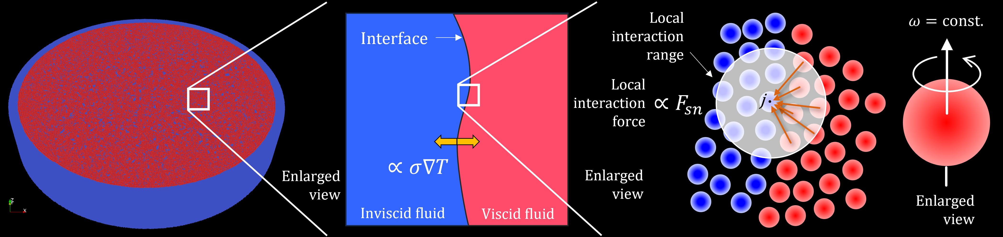
Figure 1: Schematic of our methodology: a classical mechanical interpretation of bulk liquid helium-4

In our two-fluid model, we introduce the properties of multiparticle systems as a microscopic correction as follows. First, we assume that the ratio of the number of virtual fluid particles in the inviscid and viscous components is equal to that of the quantum mechanical superfluid and normal fluid components calculated using the BEC theory at this temperature. In other words, the ratio of the number of virtual fluid particles in the inviscid and viscous components can be described as $N_{s}/N$ and $N_{n}/N$, where $N_{s}$ and $N_{n}$ are the numbers of helium atoms in the superfluid and normal flow components, respectively, and $N$ is the total number of atoms that satisfy $N_{s}+N_{n}=N$. The respective density ratios were assumed to follow BEC theory. In other words, the densities of the inviscid and viscous fluids normalized by the total density $\rho$ are $\rho_{s}/\rho$ and $\rho_{n}/\rho$, respectively, and they satisfy the relations $\rho_{s}/\rho=N_{s}/N$ and $\rho_{n}/\rho=N_{n}/N$. Thus, $\rho_{s}+\rho_{n}=\rho$. In our model, the virtual fluid particles have the same volume $V_{p}$ regardless of their particle type. Therefore, the density and mass of the fluid particles are proportional and can be expressed as $\rho_{s}=m_{s}/V_{p}$ or $\rho_{n}=m_{n}/V_{p}$, where $m_{s}$ and $m_{n}$ are the masses of the fluid particles in the inviscid and viscous fluid components, respectively. Under this physical interpretation, the total density of liquid helium remains at $\rho$ because the total mass $M$ of the fluid remains constant at any temperature and the total volume $V$ is also constant. Thus, it is reasonable to solve the system of equations for an incompressible fluid (although the use of explicit SPH also reproduces weak compressibility, as described above). The key points of our model are as follows. Let the mass of the total fluid be $M$, the density $\rho$, and the volume $V$; $\rho=M/V$. Let $\rho_{s}$ be the density of the inviscid component and $\rho_{n}$ be the density of the viscous component. Let $M_{s}$ be the total mass of the inviscid component, and $M_{n}$ be the total mass of the viscous component of the entire fluid. The relationship $\rho_{s}=M_{s}/V$ or $\rho_{n}=M_{n}/V$ holds for the entire fluid. From the relation $\rho=\rho_{s}+\rho_{n}$ $=$ $(M_{s}+M_{n})/V$ $=$ $M/V$, $M_{s}+M_{n}=M$. Accordingly, the mass $M$ is conserved throughout the system, and its component ratio is determined by the temperature $T$. The volume of the fluid is also always $V$ since the total density $\rho$ is always constant. Even if we correspond the composition ratio of the fluid particles to that of the actual microparticles, the continuum nature of the fluid is not lost.

Figure 1 presents a schematic of the proposed method. Although the two components may exhibit particle properties as described above, in principle, they are “fluid components,” and therefore, an interface between the two components is considered to exist under certain conditions. Even if the temperature of the fluid is constant, the density difference causes a temperature gradient between the two fluid particles near the interface, which acts as interfacial tension. In summary, an interfacial tension proportional to the temperature gradient is generated in the opposite direction between the two fluid components, as shown in the center of Fig.  1. In summary, the inviscid component follows the Euler equation with a temperature gradient term, whereas the viscous component follows the incompressible Navier–Stokes equation with a temperature gradient term in the opposite direction. At this stage, only the temperature gradient force contributes to the interfacial tension between the two components. Temperature is a macroscopic state quantity. In other words, only the macroscopic physical properties contribute to interfacial tension. However, as the temperature approaches absolute zero, more local interactions between the two components are expected to contribute to interfacial tension. In other words, local properties have emerged as multiparticle systems. Therefore, in addition to the macroscopic temperature gradient force, the local interaction force $\bm{\mathbf{F}}_{sn}$ between two fluid particles is explicitly described as part of the interfacial tension. In classical fluid mechanics, each phase is subjected to an action proportional to the local velocity difference between the different phases at the interface of a two-phase flow. In the Lagrangian picture, the action force between two different fluid particles is proportional to the local velocity difference between the two components. More specifically, as shown on the left-hand side of Fig. 1, the $j$th fluid particle is subjected to a force proportional to the velocity difference between its own velocity and the average of the velocities of different types of fluid particles, and its reaction force is reflected in the different types of fluid particles. Because we use the explicit SPH method described above, the interface model of the two-layer flow of the explicit SPH method can be used as is. We examined the conditions under which the interface between the two phases should be considered. First, the “interface” between the two phases is a fundamental concept in hydrodynamics. Therefore, the interface effect becomes non-negligible when the two components exhibit hydrodynamic rather than many-body properties. Liquid helium-4 is expected to behave as a uniform inviscid when no external force is applied. However, the assumption of a single-phase flow of an inviscid fluid is broken by a strong external shock or heat, and an interface effect between the two components appears. As this situation simultaneously reveals the multi-particle nature of the fluid, the interfacial effect operates only in the direction of the applied impact force, and the force does not propagate in other directions as in a continuum. In the horizontal rotation problem, liquid helium-4 was forced to rotate horizontally; therefore, fluidity with weak compressibility may manifest strongly in the horizontal direction. Accordingly, the driving force due to the temperature gradient force was assumed to act in the horizontal direction. Interface effects in this direction were not considered in our model because no external forces acted in the vertical direction.

The above can be summarized as follows. Our two-fluid model assumes mixing of inviscid and viscous fluid components. The inviscid component follows the Euler equation with a temperature gradient term, whereas the viscous component follows the incompressible Navier-Stokes equation with a temperature gradient term in the opposite direction. The interface effect between the two components owing to a temperature gradient acts in the induced direction only when classical fluidity is induced between the two components by excitation or external forces. We consider the local interaction force $\bm{\mathbf{F}}_{sn}$ acting between two different types of fluid particles that is proportional to the velocity difference between the different types of fluid particles. In addition, the viscous term was reformulated to conserve the angular momentum of the fluid particles around their axes, that is, the spin angular momentum, as previously described. The resulting system of equations is as follows [6, 7, 8]

$$\rho_{s}\frac{{\rm D}\bm{\mathbf{v}}_{s}}{{\rm D}t} = -\frac{\rho_{s}}{\rho}\nabla P+\rho_{s}\sigma\nabla T-\bm{\mathbf{F}}_{sn},$$ (1)

$$\rho_{n}\frac{{\rm D}\bm{\mathbf{v}}_{n}}{{\rm D}t} = -\frac{\rho_{n}}{\rho}\nabla P-\rho_{s}\sigma\nabla T+(\bar{\eta}+\bar{\eta_{r}})\nabla^{2}\bm{\mathbf{v}}_{n}+\biggl{(}\frac{\bar{\eta}}{3}+\bar{\xi}-\bar{\eta_{r}}\biggr{)}\nabla\nabla\cdot\bm{\mathbf{v}}_{n}+2\bar{\eta_{r}}\nabla\times\bm{\mathbf{\omega}}+\bm{\mathbf{F}}_{sn}.$$ (2)

The mathematical expressions for the three assumptions shown in Fig. 1 can be described in a form similar to that of the conventional two-fluid model derived from the $\rm Schr\ddot{o}dinger$ equation. For clarity, we make the following assumptions. (i) It is a mixture of a viscous and an inviscid fluid. (ii) The ratio of helium atoms in the ground state to the total number of atoms follows quantum statistical mechanics for bosons and thus fluctuates around its statistical average, enabling us to assume that the volume of the fluid fluctuates; in other words, weak compressibility can be assumed. (iii) Local interaction forces are exerted between two different types of fluid particles. Moreover, in another recent two-fluid model, the vortex filament model was solved instead of the inviscid equation, in which the rotation of the vortices can be considered. In contrast, we assume spin angular momentum conservation of fluid particles around their axes; thus, the viscosity term is decomposed into three terms in Eq.  (2).

Let us summarize the physical significance of each parameter in Eqs.  (1) and (2) with reference to the literature [7]. $\rho_{n}$ and $\rho_{s}$ are the mass densities of the normal and inviscid fluid components, respectively, which satisfy the relationship $\rho=\rho_{n}+\rho_{s}$, where $\rho$ is the mass density of the total fluid. $D\{\cdot\}/Dt$ denotes the material derivative. $\bm{\mathbf{v}}_{n}$ and $\bm{\mathbf{v}}_{s}$ are the velocities of normal and inviscid fluid components, respectively. $P$, $T$, and $\sigma$ denote the pressure, temperature, and entropy density, respectively. $\bar{\eta}$, $\bar{\xi}$, and $\bar{\eta_{r}}$ indicate the shear, bulk, and rotational viscosities, respectively, where $\bar{\eta_{r}}$ determines the impact of the rotational forces [10]. The fourth term on the right-hand side of Eq. (2) becomes $\rm 0$ owing to the incompressibility condition $\nabla\cdot\bm{\mathbf{v}}=0$. In this respect, the current model always imposes the incompressibility condition $\nabla\cdot\bm{\mathbf{v}}=0$, and the simulation is slightly weakly compressible by solving using the explicit SPH method. Therefore, at present, the fourth term is meaningless; however, in the future, it may be solved directly under a compressibility condition. Therefore, we describe the system of equations in a generic form as in Eq.  (2). The viscosity term in Eq. (2) is an extended version of the usual expression: the set of the third to fifth terms converges to $\bar{\eta}\nabla^{2}\bm{\mathbf{v}}_{n}$ because $\bar{\eta_{r}}$ converges to $0$ when $\nabla\cdot\bm{\mathbf{v}}=0$. This implies that $\bar{\eta}$ corresponds to the shear viscosity $\eta_{n}$ of the normal fluid. Meanwhile, the local interaction force $\bm{\mathbf{F}}_{sn}$ is expressed as follows. As mentioned earlier, $\bm{\mathbf{F}}_{sn}$ is proportional to the local velocity difference between the two components, and can be expressed as $\bm{\mathbf{F}}_{sn}=C_{l}\bm{\mathbf{v}}_{sn}$, where $C_{l}$ is a coefficient. This form exactly corresponds to the mutual friction forces between the two components in quantum mechanics; in this paper, we estimate $C_{l}$ assuming that $\bm{\mathbf{F}}_{sn}$ corresponds to the mutual friction forces $\bm{\mathbf{F}}^{q}_{sn}$ of the ordinary two-fluid model, where $\bm{\mathbf{F}}^{q}_{sn}$ can be expressed as $\bm{\mathbf{F}}^{q}_{sn}=2/3\rho_{s}\alpha\kappa L\bm{\mathbf{v}}_{sn}$, where $\bm{\mathbf{v}}_{sn}$ is the relative velocity $\bm{\mathbf{v}}_{s}-\bm{\mathbf{v}}_{n}$, $\kappa$ is the quantum of circulation, $\alpha$ is the friction coefficient, and $L$ is the time-dependent vortex line density. Unlike in our previous studies, we use the initial value of $L$ before its decay, $L^{-1}(0)$, where $L$ satisfies Vinen’s equation: $L^{-1}(t)=L^{-1}(0)+\beta_{v}t,$ where $\beta_{v}$ is a coefficient. For further details, refer to [23].

In addition, two auxiliary equations are required to solve the system of equations in Eqs. (1) and (2) such that the number of unknown independent variables equals the number of equations. Specifically, the elementary excitation model [24, 25] establishes a correlation between the entropy $\sigma$ and temperature $T$. Tait’s equation of state describes the barotropic relationship between the pressure $P$ and density $\rho$ for each fluid particle [19]:

$$\sigma \simeq \frac{1}{NM}\Biggl{[}\frac{2\pi^{2}k_{B}^{4}T^{3}}{45\hbar^{3}c^{3}}+\biggl{(}\frac{k_{B}}{2\pi}\biggr{)}^{3/2}\frac{\sqrt{\mu}p_{0}^{2}\Delta}{\hbar^{3}}\frac{e^{-\Delta/T}}{\sqrt{T}}\Biggr{]},$$ (3)

$$P = p_{0}\Biggl{(}\frac{\rho}{\rho_{0}}\Biggr{)}^{\alpha_{P}}-\beta_{P}.$$ (4)

Let us explain the physical significance of each parameter in Eqs.  (3) and (4) with reference to Refs.  [6, 7]. In Eq. (3), $M$ represents the mass of a helium-4 atom, $N$ indicates the total number of helium-4 atoms in the system, $\pi$ represents the circumference of the circle, and $c$ is the speed of sound. $\hbar$ indicates the reduced Planck’s constant and $k_{B}$ represents the Boltzmann constant. The constant values $\mu$, $p_{0}$, and $\Delta$ are given by ${\rm 1.72\times 10^{-24}~{}g}$, ${\rm 2.1\times 10^{-19}~{}gcms^{-1}}$, and ${\rm 8.9~{}K}$, respectively  [25, 26]. Eq. (3) is always true within the scope of this study because it is valid if $T\ll{\rm 93~{}K}$ [25]. In the elementary excitation model, the first term in the parentheses on the right side of Eq. (3) represents the “photon” contribution, and the second term in the same parentheses represents the “roton” contribution; after finding the total pressure from the summation of the photon and roton contributions, the entropy density in Eq. (3) is obtained by the thermodynamic relation, such that the partial derivative of pressure with respect to temperature [6]. Equation (3) represents the relationship between entropy density $\sigma$ and temperature $T$ in a quantum “ideal gas.” To obtain the value of liquid helium-4, we decompose $\sigma$ as $\sigma=C_{e}\sigma_{0}$, where $C_{e}$ indicates the volume ratio of liquid to gaseous helium-4 under an atmospheric pressure of $\rm 1.01325~{}bar$, which is $1.428\times 10^{-3}$ [27]. Under constant temperature, we calculated $\sigma_{0}$ using Eq.  (3) and maintained a constant value for entropy conservation. Meanwhile, in Eq. (4), $\rho_{0}$ and $p_{0}$ represent the fluid density and pressure in the initial state, respectively. $\alpha_{P}$ is the specific heat ratio that affects system incompressibility. $\beta_{P}$ denotes the reference pressure, which typically corresponds to $p_{0}$. Equations (1)–(4) represent the governing equations of the system.

2.2 Multi-GPU computing for large-scale particle simulations

In high-performance computing, an effective parallel computing algorithm for the simulation of many-particle interacting systems should be chosen based on the characteristics of the target problem, computational scheme, and properties of the parallel computing environment. In general, these problems include gravitational many-body problems [28, 29], molecular dynamics (MD) problems [30, 31, 32], Lagrangian fluid analysis using SPH [33, 34], deformation analysis of structures using the mesh-free method [35, 36, 37, 38, 39], and powder problems using the distinct element method (DEM) [40, 41, 42, 43]. The interaction domains and connectivity between particles depend on the target problem. From a computational perspective, gravitational many-body problems and MD problems result in N-body calculations owing to the large interaction range. Consequently, the computational cost of the interaction calculations is $O(N^{2})$. Conversely, DEM calculations for powders require interaction calculations of the repulsion and friction between the contacting particles. Therefore, the memory reference cost is more significant than the computational cost when appropriate techniques such as neighbor particle listing and particle data sorting [44, 45, 46] are implemented to reduce the interaction calculation cost to $O(N)$. In contrast, fluid calculations using particle methods, such as SPH, stand at a middle ground between the N-body and DEM calculations in terms of both memory reference and computational cost, even if we use a technique similar to DEM. In a 3D calculation, each particle interacts with approximately a few hundred particles within the interaction domain, which is called the kernel radius. Moreover, the numerical accuracy of the spatial discretization in SPH is typically equivalent to that of the central difference method in the finite difference method (FDM). In addition, the time discretization accuracy was between the first- and second-order accuracies with respect to the resolution, depending on the time-integration schemes. Accordingly, it is imperative to capture the underlying real physics with the highest possible accuracy using as many analytical particles as possible. This is one of the reasons why the field of large-scale simulation of particle methods frequently appears in the ACM Gordon Bell Prize [47].

In recent years, graphics processing units (GPUs) have been installed in world-class supercomputers as accelerators to improve the computational performance, memory utilization, power efficiency, and other metrics. Multi-GPU computing can speed up simulations and ensure that sufficient memory is available. The development of applications that operate efficiently on GPU supercomputers requires CUDA programming [48]. This also requires making good use of hierarchical memory structures, such as the limited amount of device memory on the GPU board and high-speed shared memory on the chip. The GPU supercomputer consists of many nodes with distributed memory connected by high-speed networks. GPUs are installed on each compute node as computational accelerators. For particle simulations on a memory-distributed system such as a supercomputer, it is efficient to divide the entire computational domain in space and assign a node with accelerators to each divided subdomains. Among particle problems, calculations performed in gravitational many-body and MD are based on long-range interactions. Therefore, the computational cost is dominated by floating-point operations rather than memory accesses, which allows for high execution performance, even on GPU supercomputers with low byte/flops. However, in SPH simulations that compute short-range interactions, most computational time is spent on memory accesses, making it impossible for a low byte/flop supercomputer to achieve sufficient performance.

The computational cost per GPU for particle simulations using SPH depends on the number of particles in the subdomains to which each GPU is assigned. In a parallel computing platform such as a supercomputer, the distribution of particles among nodes changes in both time and space, resulting in a non-uniform distribution of particles per node. At this point, the computational load in regions that are densely populated with particles increases significantly, making large-scale computations impractical. Therefore, it is essential to introduce dynamic load balancing between nodes to achieve sufficient execution performance in simulations of short-range interaction-based particle methods, such as SPH. This involves repartitioning the computational domain according to particle distribution to ensure that the computational load on each node is uniform. However, achieving dynamic load balancing in simulations of short-range interaction-based particle methods on GPU supercomputers is challenging because of hierarchical memory structures. The implementation is further complicated by the need for specialized technologies specific to large-scale parallel computing, such as CUDA programming and the MPI library [49], for the development of the computational code. In addition, when the particle distribution undergoes significant changes and moves in a random direction across nodes, it is essential to efficiently manage the particle data on the GPUs to minimize the communication cost between GPUs across nodes via host CPUs and between GPUs and CPUs within each node. It is critical to consider efficient computation methods for individual GPUs considering their different memory structures, such as the device memory on the GPU and the high-speed shared memory on the chip.

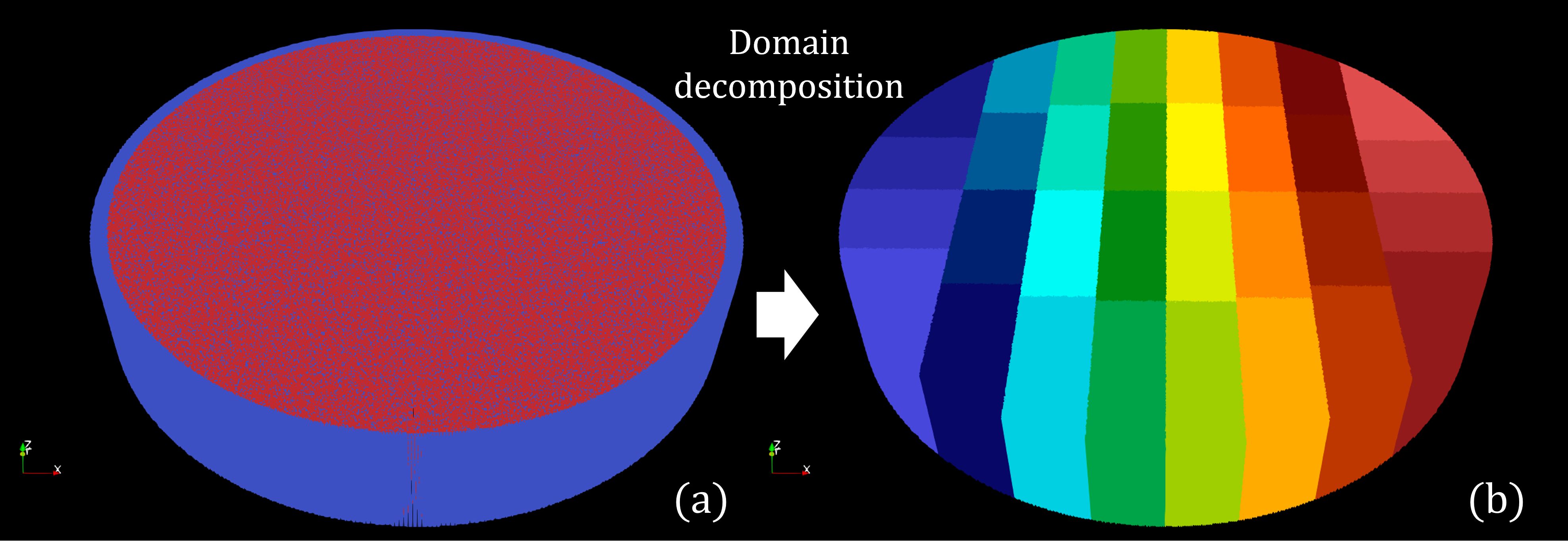
Figure 2: Snapshots of particle distribution (left part) and the domain decomposition in the case where approximately 19.6 million fluid particles were divided into 32 subdomains, each of which was assigned to a single GPU.

It is imperative to develop dynamic load balancing among the GPUs to exploit the high computational efficiency of multiple GPUs. Various load balancing techniques have been proposed in related fields, including the slice-grid method, which moves the domain boundary to a spatially partitioned region; graph theory-based partitioning (such as k-means), as represented by ParMETIS [50, 51] and Zoltan [52, 53]; and the hierarchically structured tree method, which uses a recursive structure of cells to partition a domain, as exemplified by kd-tree decomposition [54], orthogonal recursive bisection (ORB) [55, 56, 57], and domain decomposition using a hierarchically structured grid with space-filling curves [58]. Recently, we conducted a study on optimal dynamic domain decomposition for particle simulations of short-range interactions compatible with low byte/flops supercomputers, such as GPU supercomputers. Subsequently, we developed a multi-GPU computing framework that enables large-scale particle simulations using SPH. The SPH computational framework [46] developed by the author was used in this study. Based on the nature of the target problem, the 2D slice grid method was used as the domain decomposition method. Figure 2 illustrates a snapshot of the domain decomposition in the case where the 19.5 million fluid particles were divided into 32 subdomains, each of which was assigned to a single GPU to speed up the simulations.

Unlike the free surface problem, the particle distribution in the rotating liquid helium-4 simulation was not excessively biased. Therefore, to prevent the computational load from being excessively biased, we divided the domain at regular intervals, such as every several hundred steps, so that the overhead of domain re-segmentation was negligible, and the load was balanced. A workflow diagram of the calculations is presented in Algorithm 1. The SPH calculation process for the 3D simulation of liquid helium-4 using our two-fluid model was, in principle, the same as that for the 2D case reported in our previous study. The velocity Verlet method [59, 60] was used as the time integration method, and a nonslip condition was imposed on the lateral wall boundaries. As this is a three-dimensional calculation, a slip condition is imposed on the top and bottom surfaces, assuming that the inviscid fluid continues. After the particle density was calculated, the particle pressure was determined using the Tait’s equation of state. After applying the pressure filter [61], the updated particle density and particle pressure were used to calculate the pressure and temperature gradient forces. The viscosity term was separately calculated for the rotational and shear viscosities of the particles. The collision model [62] computed in line 17 is a correction model that preserves the volume effect of the fluid particles. The local interaction forces between the viscous and inviscid fluid particles were then computed alternately, the boundary conditions were calculated, and the physical quantities of the particles were updated according to the velocity Verlet algorithm. For the detailed description of the computational model using SPH, please refer to Refs. [6, 7].

Algorithm 1 Computational workflow for simulations using our SPH model on a multi-GPU platform

1:for ${\tt j}$ = 0 $\to$ ${\tt N_{step}}$ do

2:    Re-decompose the domain using the 2D slice-grid method (at a fixed interval).

3:    Construct Neighbor Particle Lists (NPLs) in each subdomain.

4:    for ${\tt k}$ = 0 $\to$ ${\tt N_{velver}}$ do

5:         Communicate the halo particles (all particles in the halo).

6:         Register particles in the NPLs.

7:         if k $=$ second step then

8:             Compute the particle densities.

9:             Compute the particle pressures.

10:             Communicate the halo particles (only updated particles in the halo).

11:             Compute the pressure filter.

12:         end if

13:         Communicate the halo particles (only updated particles in the halo).

14:         Compute the pressure gradient forces.

15:         Compute the temperature gradient forces.

16:         Compute the viscosity forces.

17:         Compute collisions.

18:         Compute local interaction forces (from viscid to inviscid).

19:         Communicate the halo particles (only updated particles in the halo).

20:         Compute local interaction forces (from inviscid to viscid).

21:         Calculate boundary conditions (from fluid to wall particles).

22:         Communicate the halo particles (only updated particles in the halo).

23:         Calculate boundary conditions (from wall to fluid particles).

24:         Calculate time integration (update using Velocity Verlet method).

25:         Communicate out-of-domain particles.

26:    end for

27:    Defragment GPU memory (at a fixed interval).

28:end for

Given the significant increase in the computational cost associated with 3D calculations, it is imperative to run simulations on a multi-GPU platform. As previously mentioned, dividing the computational domain into subdomains and assigning a GPU to each subdomain is a highly efficient approach. To ensure the connectivity of the domains between subdomains, it is necessary to copy the updated particle data to the neighboring subdomains each time the particles are in the halo region, which is between the boundaries with the neighboring domain and the interior of the domain by the interaction length (in our implementation, twice the kernel radius), update their properties. As shown in Algorithm 1, five communications of particle data within the halo domain were required. In addition, the particle positions are updated after all computations in a single step were completed. Each GPU then transfers the out-of-domain particles that have left the subdomain to the target neighboring subdomain. Consequently, communication between neighboring GPUs was required six times. Frequent repetition of communication fragments the particle array and reduces the performance; therefore, periodic reordering of particle data is performed. This process enables efficient multi-GPU computation using SPH.

3 Large-scale simulations of horizontally rotating 3D liquid helium-4

Let us set the outer diameter of a cylindrical container in the horizontal direction to 0.2 cm with a thickness of 0.04 in the vertical direction (z-direction). The resolutions of $(N_{x},N_{y},N_{z})$ are given by (500, 500, 100), where $N_{a}$ $(a=x,y,z)$ indicates the number of particles in the direction in a rectangular domain that covers the cylindrical container. We set the rotational angular velocity around the cylinder axis (z axis) to 5 rad $\cdot s^{-1}$ counterclockwise. Similar to the two-dimensional cases in our previous work, we set the temperature T to 1.6 K and determined the values of $(\rho_{s}/\rho,\rho_{n}/\rho,\kappa)$ with those at T = 1.6 K listed in Ref. [63]. In addition, $\eta_{n}$ was obtained from the relationship of 0.566 $\kappa\rho_{n}$ with reference to [63]. The shear viscosity $\bar{\eta}$ and rotational viscosity $\bar{\eta_{r}}$ have the value of $\eta_{n}$. We set the parameter $C_{\omega}$, which determines the magnitude of the angular velocity $\omega$ and thereby determines the resulting number of vortices, to be 0.016 to maintain a similar degree of magnitude of the rotational forces as those in 2D cases reported in our previous studies. Normal fluid particles were placed along the inner circumference of the container as walls, and no-slip conditions were imposed on the wall particles as boundary conditions. Conversely, we set slip conditions at the top and bottom of the vessel. In the initial state, superfluid or normal fluid particles were randomly generated in proportion to the density ratio and distributed in the vessel. We set dt to $5.0\times 10^{-6}$ s and computed 180000 time steps, which is 0.9 s in physical time. In the simulation, under the aforementioned conditions, the total number of normal and inviscid fluid particles, including the wall particles, was 19636400. We boosted our simulation using 32 GPUs installed on the Wisteria/BDEC-01 supercomputer at The University of Tokyo, JAPAN. We applied a two-dimensional slice-grid technique to the dynamic domain decomposition in the horizontal direction and decomposed the computational domain into 32 subdomains (four in the horizontal direction and eight in the depth direction), and a single GPU was assigned to each subdomain. Consequently, approximately 5.5 days were required to compute all 180000 time steps of the simulation. For comparison, we performed simulations with a lower resolution using $(N_{x},N_{y},N_{z})$ = (250, 250, 50) to investigate the dependence of the observed phenomena on the computational resolution.

Figure 3 shows snapshots of the rotation simulation with a lower resolution using 2454000 particles from the beginning to 0.79 s in physical time. The fluid particles of the inviscid and viscous components were visualized in color according to the strength of the rotational forces calculated by the fifth term of Eq. (2) using the volume rendering technique. The wall particles were removed for visualization. A video of the simulation is presented in Fig. 3 as integral multimedia in Fig. 4. A preprint version of the video is available at
(https://www.satoritsuzuki.org/video-horizontally-rotated-3d4he-2p4m). A single forced vortex that spans the container is generated in the rotation problem of a single-phase flow in classical fluid mechanics. However, it can be confirmed that the behavior of the fluid is similar to that of a quantum fluid. In other words, we observed that the low-density and viscous components coalesced to form multiple spinning vortices. By contrast, in this simulation, the vortices repeat arbitrary coupling and separation while continuously changing. This is characteristic of classical fluids. It is reasonable that the dynamics of the vortex should be similar to those of classical flow because it does not currently contain artificial rules for vortex recombination, as observed in quantum fluids. In the future, if, for example, K. W. Schwarz’s rule [13, 14] is introduced, it will be possible to get closer to the second image of the quantum vortex. Snapshots from the beginning of the simulation to 0.79 s in physical time in the high-resolution case with approximately 19.6 million particles are shown in Fig. 5. A video of the simulation is presented in Fig. 5 is provided as integral multimedia in Fig. 6. A preprint version of the video is available at (https://www.satoritsuzuki.org/video-horizontally-rotated-3d4he-19m). Low-density and viscous components agglomerate to form multiple spinning vortices, which is common in the low-resolution case. This is also the same as in the low-resolution case in that the vortices experience arbitrary connection and separation with continuous change. However, unlike in the low-resolution case, the individual vortices are thinner and the number of vortices is larger, even though the computational conditions are the same.

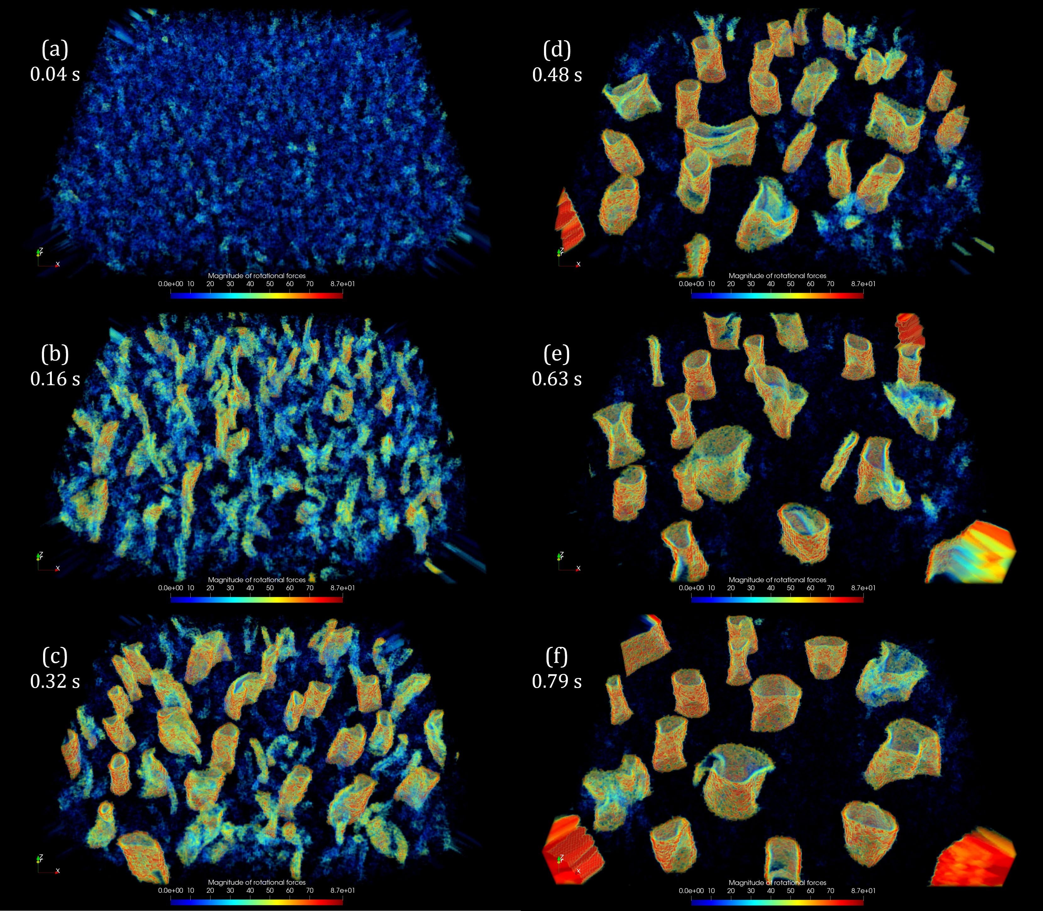
Figure 3: Snapshots of the rotation simulation with the lower resolution using 2454000 particles from the beginning to 0.79 s in physical time.

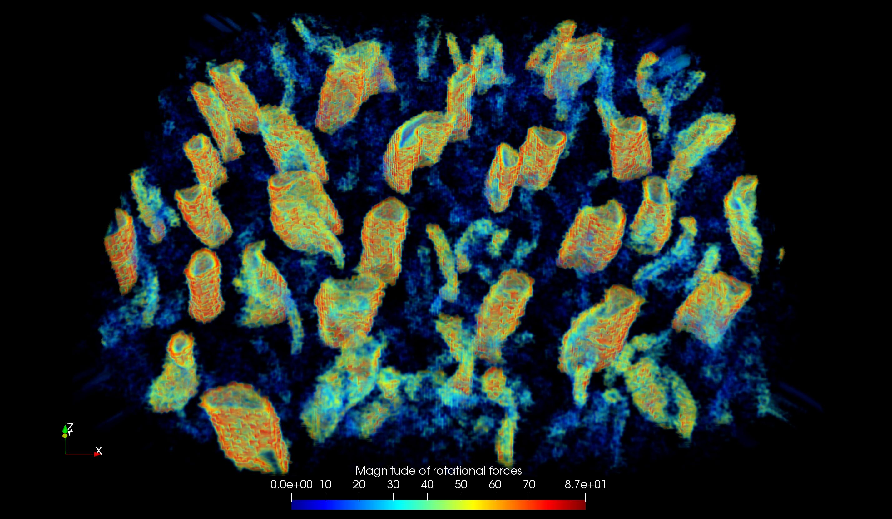
Figure 4: A video of the snapshots in Fig. 3 (Multimedia view)

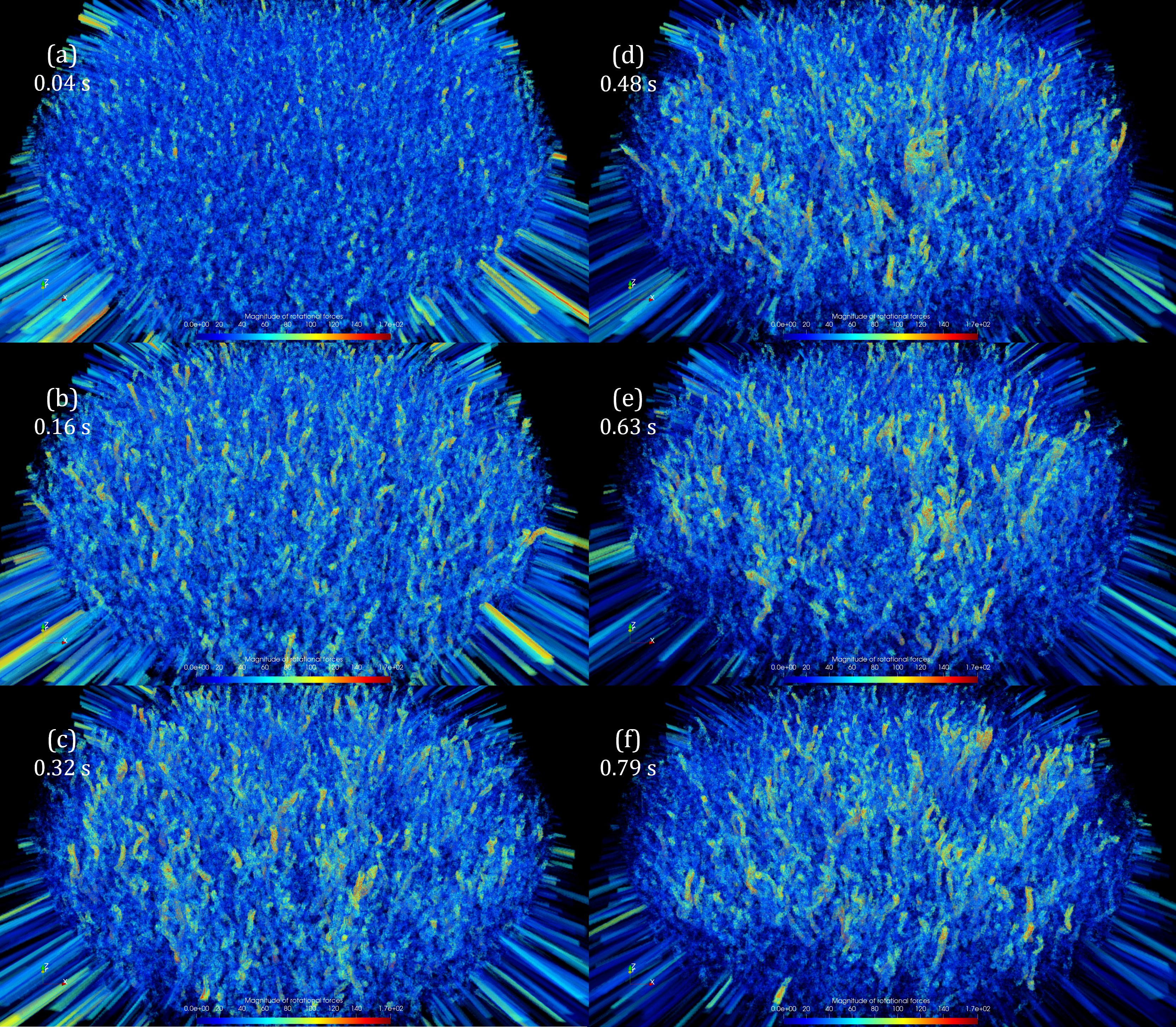
Figure 5: Snapshots of the rotation simulation with the higher resolution using 19636400 particles from the beginning to 0.79 s in physical time.

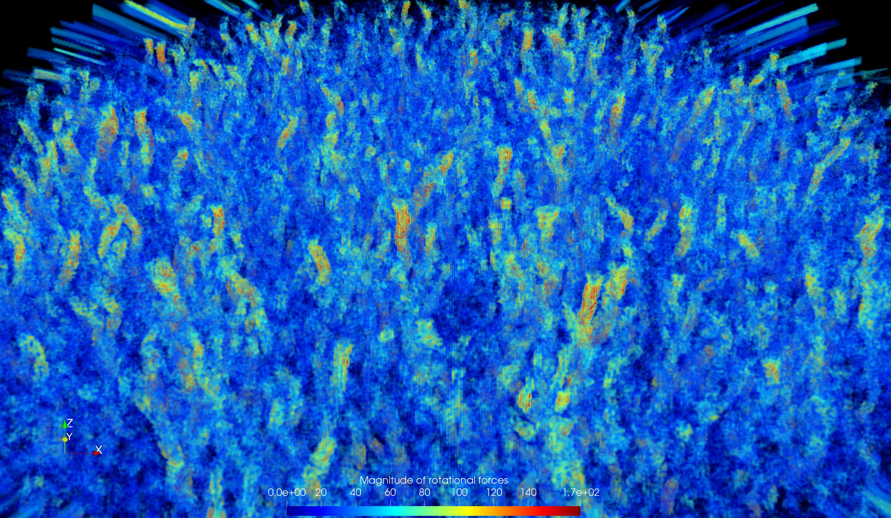
Figure 6: A video of the snapshots in Fig. 5 (Multimedia view)

4 Discussion

A description of the dynamics of liquid helium-4 at cryogenic temperatures based on classical fluid dynamics yields Eqs.  (1) and (2), which are similar to the conventional two-fluid model derived by combining the nonlinear $\rm Schr\ddot{o}dinger$ equation for bosons, that is, the Gross-Pitaevskii equation, with the thermodynamic relation Gibbs-Duhem equation. In addition, our two-fluid model includes a conservation term for angular momentum related to the rotation of classical fluid particles. The fact that we could reproduce multiple spinning vortices, such as quantum vortices, using a method based on classical fluid mechanics would be groundbreaking because multiple spinning vortices and their lattice phenomena in liquid helium-4 were thought to originate purely from quantum mechanics. The simulation results showed that the individual vortices were thinner and that there were more vortices in the high-resolution simulation than in the low-resolution simulation. This is reasonable because if we focus on the cross section at z = 0, the number of vortices observed on the cross section should be a few hundred according to Feynman’s law in two-dimensional cases [7]. In addition, the vortex centers of quantum vortices are essentially of the order of angstroms (although quantum vortices are thought to interact even at large distances). Therefore, the results of the high-resolution simulation were closer to the theoretical solution.

As mentioned previously, the usual two-fluid model and our fluid model have the same form of equations, but their interpretations differ. Usually, the two components–superfluid and normal flow–overlap, and the interaction between them is interpreted as occurring only through the mutual friction term. In other words, these two components coexist in a single region. This is a quantum mechanical picture. However, our model considers liquid helium as an inviscid fluid in a continuum, with a viscous component remaining at finite temperatures. The two components interact as a multiphase flow under certain conditions; however, the nature of a multiparticle system appears locally. In this case, the temperature gradient along the horizontal direction was considered. In addition, a local interaction force proportional to the velocity difference, which is often used in particle-fluid coupling, acts between the two-fluid particles (we also call this the mutual friction force because it has the same form as the quantum mechanical mutual friction force). Thus, multiphase flow and particle-fluid coupling are often modeled according to classical fluid mechanics. Because the fluid particles are only fragments of continuum mechanics, they do not overlap and exhibit an excluded volume effect on each other. In summary, unlike the typical two-fluid model, our two-fluid model, which is based on classical fluid mechanics, is a one-fluid system. In this sense, it makes sense that high-resolution simulations approach the quantum mechanical picture more closely than low-resolution simulations. In multiparticle simulations, the computational resolution is determined by the diameter of the fluid particles. As the computation increases in resolution, the fluid particles decrease in size. Simultaneously, the excluded volume effect of the fluid particles also decreased; therefore, the particles were more likely to slip through and overlap with each other. Consequently, our method describes a one-fluid system at a low resolution, in which the two components are separated to describe a single fluid. However, as the resolution increases, the system is expected to become a two-fluid system. In other words, we can expect our two-fluid model to be smoothly connected and equal to the two-fluid model. That is, in this problem, the convergence of the calculations coincides with the convergence of the physical phenomena.

In our model, the fluid particles were subjected to pressure gradient forces, temperature gradient forces, shear viscosity, rotational viscosity, and mutual friction forces. The shear and rotational viscous forces act only between the components of the viscous fluid. In a typical case, the distribution of these forces acting on the fluid particles was approximately 72.9 % pressure gradient force, 8.28 % temperature gradient force, 18.07 % shear viscous force, and approximately 0.71 % rotational viscous force. The mutual friction force was approximately 0.01 %–0.04 % that of the rest. Although the rotational viscous force is less than 1 % of the force applied to the fluid particles, it is understandable that it causes an independently spinning vortex. The mutual frictional force is negligible but may act as a disturbance, and which force induces which physical phenomena should be investigated in future studies.

5 Conclusion

In this paper, we report a 3D simulation of the rotating liquid helium-4 using a two-fluid model with spin-angular momentum conservation using SPH. The conventional two-fluid model was derived by combining the nonlinear Schrodinger equation for bosons with the thermodynamic Gibbs-Duhem equation. In short, the usual two-fluid model is obtained by making macro-corrections to the microscopic relational equations. In contrast, our model is derived from the particle approximation of an inviscid fluid with residual viscosity in part. Despite the fully classical mechanical picture, the resulting system equations were consistent with those of the conventional two-fluid model. Specifically, we consider the bulk liquid helium-4 to be an inviscid fluid, assuming that the viscous fluid component remains at finite temperatures. As the temperature decreased, the amount of the viscous fluid component decreased, ultimately becoming a fully inviscid fluid at absolute zero. Weak compressibility is assumed to express the volume change because some helium atoms do not render fluid owing to BECs or change states owing to local thermal excitation. Using explicit SPH (smoothed particle hydrodynamics), one can solve the governing equations for an incompressible fluid, simultaneously reproducing density fluctuations and describing the fluid in a many-particle system. We assume the following fluid-particle duality: a hydrodynamic interfacial tension between the inviscid and viscous components or a local interaction force between two types of fluid particles. The former can be induced in the horizontal direction when non-negligible non-uniformity of the particles occurs during forced 2D rotation, and the latter is non-negligible when the former is negligible. We performed a large-scale simulation of 3D liquid helium forced to rotate horizontally using 32 GPUs. Compared with the low-resolution calculation using 2.4 million particles, the high-resolution calculation using 19.6 million particles showed spinning vortices close to those of the theoretical solution. In the future, the introduction of quantum mechanical recombination among vortices will capture the behavior of quantum fluids. We obtained a promising venue to establish a practical simulation method for bulk liquid helium-4.

References

- [1] V. M. Arzhavitin, Diffusion mechanism of internal friction in a niobium–titanium alloy, Russian Metallurgy (Metally) 2016, 431 (2016).
- [2] N. Banno, Low-temperature superconductors: Nb3sn, nb3al, and nbti, Superconductivity 6, 100047 (2023).
- [3] A. T. Jones, R. B. E. Down, C. R. Lawson, D. Keeping, and O. Kirichek, Carbon footprint of helium recovery systems, Low Temperature Physics 49, 967 (2023), https://pubs.aip.org/aip/ltp/article-pdf/49/8/967/18070432/967_1_10.0020164.pdf.
- [4] L. H. Wilson, The Viscosity of Gases, PhD thesis, 1950.
- [5] I. L. FabelinskiÄ, Macroscopic and molecular shear viscosity, Physics-Uspekhi 40, 689 (1997).
- [6] S. Tsuzuki, Particle approximation of the two-fluid model for superfluid 4he using smoothed particle hydrodynamics, Journal of Physics Communications 5, 035001 (2021).
- [7] S. Tsuzuki, Reproduction of vortex lattices in the simulations of rotating liquid helium-4 by numerically solving the two-fluid model using smoothed-particle hydrodynamics incorporating vortex dynamics, Physics of Fluids 33, 087117 (2021), https://doi.org/10.1063/5.0060605.
- [8] S. Tsuzuki, Theoretical framework bridging classical and quantum mechanics for the dynamics of cryogenic liquid helium-4 using smoothed-particle hydrodynamics, Physics of Fluids 34, 127116 (2022), https://doi.org/10.1063/5.0122247.
- [9] D. W. Condiff and J. S. Dahler, Fluid mechanical aspects of antisymmetric stress, The Physics of Fluids 7, 842 (1964).
- [10] K. Müller, D. A. Fedosov, and G. Gompper, Smoothed dissipative particle dynamics with angular momentum conservation, Journal of Computational Physics 281, 301 (2015).
- [11] R. A. Gingold and J. J. Monaghan, Smoothed particle hydrodynamics: theory and application to non-spherical stars, Monthly notices of the royal astronomical society 181, 375 (1977).
- [12] J. J. Monaghan, Smoothed particle hydrodynamics, Annual review of astronomy and astrophysics 30, 543 (1992).
- [13] K. W. Schwarz, Three-dimensional vortex dynamics in superfluid : Line-line and line-boundary interactions, Phys. Rev. B 31, 5782 (1985).
- [14] K. W. Schwarz, Three-dimensional vortex dynamics in superfluid : Homogeneous superfluid turbulence, Phys. Rev. B 38, 2398 (1988).
- [15] L. TISZA, Transport phenomena in helium ii, Nature 141, 913 (1938).
- [16] L. Landau, Theory of the superfluidity of helium ii, Phys. Rev. 60, 356 (1941).
- [17] C. Gorter and J. Mellink, On the irreversible processes in liquid helium ii, Physica 15, 285 (1949).
- [18] V. F. Sears, E. C. Svensson, P. Martel, and A. D. B. Woods, Neutron-scattering determination of the momentum distribution and the condensate fraction in liquid , Phys. Rev. Lett. 49, 279 (1982).
- [19] J. J. Monaghan, Smoothed particle hydrodynamics, Reports on Progress in Physics 68, 1703 (2005).
- [20] M. Becker and M. Teschner, Weakly compressible sph for free surface flows, in Proceedings of the Eurographics symposium on Computer animation, pp. 209–217, Eurographics Association, 2007.
- [21] J. Monaghan, Simulating free surface flows with sph, Journal of Computational Physics 110, 399 (1994).
- [22] Nomeritae, E. Daly, S. Grimaldi, and H. H. Bui, Explicit incompressible sph algorithm for free-surface flow modelling: A comparison with weakly compressible schemes, Advances in Water Resources 97, 156 (2016).
- [23] S. K. Nemirovskii, Quantum turbulence: Theoretical and numerical problems, Physics Reports 524, 85 (2013), Quantum Turbulence: Theoretical and Numerical Problems.
- [24] I. N. Adamenko, K. E. Nemchenko, I. V. Tanatarov, and A. F. G. Wyatt, Pressure of thermal excitations in superfluid helium, Journal of Physics: Condensed Matter 20, 245103 (2008).
- [25] A. Schmitt, Introduction to superfluidity, Lect. Notes Phys 888 (2015).
- [26] K.-H. Bennemann and J. B. Ketterson, Novel superfluidsvolume 1 (OUP Oxford, 2013).
- [27] C. Hammond, The elements, Handbook of chemistry and physics 81 (2000).
- [28] T. Ishiyama, K. Nitadori, and J. Makino, 4.45 pflops astrophysical n-body simulation on k computer: the gravitational trillion-body problem, in Proceedings of the International Conference on High Performance Computing, Networking, Storage and Analysis, SC ’12, Washington, DC, USA, 2012, IEEE Computer Society Press.
- [29] D. Sugimoto et al., A special-purpose computer for gravitational many-body problems, Nature 345, 33 (1990).
- [30] J. C. Phillips et al., Scalable molecular dynamics with namd, Journal of Computational Chemistry 26, 1781 (2005).
- [31] M. Valiev et al., Nwchem: A comprehensive and scalable open-source solution for large scale molecular simulations, Computer Physics Communications 181, 1477 (2010).
- [32] A. Heinecke, W. Eckhardt, M. Horsch, and H.-J. Bungartz, Parallelization of MD Algorithms and Load Balancing (Springer International Publishing, Cham, 2015), pp. 31–44.
- [33] Z. Zhang et al., Swsph: A massively parallel sph implementation for hundred-billion-particle simulation on new sunway supercomputer, in Euro-Par 2023: Parallel Processing, edited by J. Cano, M. D. Dikaiakos, G. A. Papadopoulos, M. Pericàs, and R. Sakellariou, pp. 564–577, Cham, 2023, Springer Nature Switzerland.
- [34] G. Oger et al., On distributed memory mpi-based parallelization of sph codes in massive hpc context, Computer Physics Communications 200, 1 (2016).
- [35] J.-S. Chen, C. Pan, C.-T. Wu, and W. K. Liu, Reproducing kernel particle methods for large deformation analysis of non-linear structures, Computer Methods in Applied Mechanics and Engineering 139, 195 (1996).
- [36] B. Nayroles, G. Touzot, and P. Villon, Generalizing the finite element method: Diffuse approximation and diffuse elements, Computational Mechanics 10, 307 (1992).
- [37] T. Belytschko, Y. Y. Lu, and L. Gu, Element-free galerkin methods, International Journal for Numerical Methods in Engineering 37, 229 (1994).
- [38] Z. Lin, D. Wang, D. Qi, and L. Deng, A petrov-galerkin finite element-meshfree formulation for multi-dimensional fractional diffusion equations, Computational Mechanics 66, 323 (2020).
- [39] M. Sakai, Y. Mori, X. Sun, and K. Takabatake, Recent progress on mesh-free particle methods for simulations of multi-phase flows: A review, KONA Powder and Particle Journal 37, 132 (2020).
- [40] P. A. Cundall and O. D. L. Strack, A discrete numerical model for granular assemblies, Géotechnique 29, 47 (1979).
- [41] E. H. Park, V. Kindratenko, and Y. M. Hashash, Shared memory parallelization for high-fidelity large-scale 3d polyhedral particle simulations, Computers and Geotechnics 137, 104008 (2021).
- [42] B. Yan and R. A. Regueiro, A comprehensive study of mpi parallelism in three-dimensional discrete element method (dem) simulation of complex-shaped granular particles, Computational Particle Mechanics 5, 553 (2018).
- [43] J. Gan, T. Evans, and A. Yu, Application of gpu-dem simulation on large-scale granular handling and processing in ironmaking related industries, Powder Technology 361, 258 (2020).
- [44] G. S. Grest, B. Dünweg, and K. Kremer, Vectorized link cell fortran code for molecular dynamics simulations for a large number of particles, Computer Physics Communications 55, 269 (1989).
- [45] M. Gomez-Gesteira et al., Sphysics - development of a free-surface fluid solver - part 2: Efficiency and test cases, Comput. Geosci. 48, 300â307 (2012).
- [46] S. Tsuzuki and T. Aoki, Effective dynamic load balance using space-filling curves for large-scale sph simulations on gpu-rich supercomputers, in Proceedings of the 7th Workshop on Latest Advances in Scalable Algorithms for Large-Scale Systems, ScalA ’16, pp. 1–8, Piscataway, NJ, USA, 2016, IEEE Press.
- [47] G. Bell, D. H. Bailey, J. Dongarra, A. H. Karp, and K. Walsh, A look back on 30 years of the gordon bell prize, The International Journal of High Performance Computing Applications 31, 469 (2017).
- [48] D. Luebke, Cuda: Scalable parallel programming for high-performance scientific computing, in 2008 5th IEEE International Symposium on Biomedical Imaging: From Nano to Macro, pp. 836–838, 2008.
- [49] Message Passing Interface Forum, MPI: A Message-Passing Interface Standard Version 4.1, 2023.
- [50] G. Karypis and V. Kumar, A fast and high quality multilevel scheme for partitioning irregular graphs, SIAM Journal on Scientific Computing 20, 359 (1998).
- [51] G. Karypis, METIS and ParMETIS (Springer US, Boston, MA, 2011), pp. 1117–1124.
- [52] K. Devine, E. Boman, L. Riesen, U. Catalyurek, and C. Chevalier, Getting started with zoltan: A short tutorial, in Proc. of 2009 Dagstuhl Seminar on Combinatorial Scientific Computing, 2009, Also available as Sandia National Labs Tech Report SAND2009-0578C.
- [53] K. Devine, E. Boman, R. Heapby, B. Hendrickson, and C. Vaughan, Zoltan data management service for parallel dynamic applications, Computing in Science and Engg. 4, 90â97 (2002).
- [54] R. Trobec and M. Depolli, A k-d tree based partitioning of computational domains for efficient parallel computing, in 2021 44th International Convention on Information, Communication and Electronic Technology (MIPRO), pp. 284–290, 2021.
- [55] J. Dubinski, A parallel tree code, New Astronomy 1, 133 (1996).
- [56] P. Liu and S. Bhatt, Experiences with parallel n-body simulation, Parallel and Distributed Systems, IEEE Transactions on 11, 1306 (2001).
- [57] M. Reumann et al., Orthogonal recursive bisection data decomposition for high performance computing in cardiac model simulations: Dependence on anatomical geometry, in 2009 Annual International Conference of the IEEE Engineering in Medicine and Biology Society, pp. 2799–2802, 2009.
- [58] S. Aluru and F. E. Sevilgen, Parallel domain decomposition and load balancing using space-filling curves, in Proceedings Fourth International Conference on High-Performance Computing, pp. 230–235, IEEE, 1997.
- [59] L. Verlet, Computer ”experiments” on classical fluids. i. thermodynamical properties of lennard-jones molecules, Phys. Rev. 159, 98 (1967).
- [60] M. P. Allen and D. J. Tildesley, Computer Simulation of Liquids (Clarendon Press, USA, 1989).
- [61] Y. Imoto, S. Tsuzuki, and D. Nishiura, Convergence study and optimal weight functions of an explicit particle method for the incompressible navier–stokes equations, Computational Particle Mechanics 6, 671 (2019).
- [62] A. Shakibaeinia and Y.-C. Jin, Mps mesh-free particle method for multiphase flows, Computer Methods in Applied Mechanics and Engineering 229-232, 13 (2012).
- [63] W. F. Vinen and J. J. Niemela, Quantum turbulence, Journal of Low Temperature Physics 128, 167 (2002).