aainstitutetext: Department of Physics “Giuseppe Occhialini”, University of Milano-Bicocca,
Piazza della Scienza 3, I-20126 Milano, Italy
bbinstitutetext: INFN Milano–Bicocca,
Piazza della Scienza 3, I-20126 Milano, Italy
ccinstitutetext: AEC, Institute for Theoretical Physics, University of Bern,
Sidlerstrasse 5, CH-3012 Bern, Switzerland

Baryonic thermal screening mass at NLO

Leonardo Giusti leonardo.giusti@unimib.it c    M. Laine laine@itp.unibe.ch a,b    Davide Laudicina d.laudicina1@campus.unimib.it b    Michele Pepe michele.pepe@mib.infn.it a,b    Pietro Rescigno p.rescigno1@campus.unimib.it
Abstract

We determine the resummed 1-loop correction to a baryonic thermal screening mass. The calculation is carried out in the framework of a dimensionally reduced effective theory, where quarks are heavy fields due to their non-zero Matsubara frequencies. The correction due to interactions is computed at O($g^{2}$) in the coupling constant. In order to solve a 3-body Schrödinger equation, we exploit a two-dimensional generalization of the hyperspherical harmonics method. At electroweak scale temperatures, the NLO correction represents a $\sim 4.6\%$ increase of the free-theory value $3\pi T$ of the screening mass.

1 Introduction

The dynamics of QCD at high temperatures plays a rôle in a number of physical processes, ranging from the cosmological evolution of the universe a few microseconds after the Big Bang, to the interpretation of empirical data from heavy ion collision experiments. Due to asymptotic freedom, one may hope that at high enough temperatures, the influence of interactions can be incorporated via a weak-coupling expansion. However, QCD effectively behaves as a three-dimensional Yang-Mills theory in this regime Linde:1980ts , which displays confinement. This implies that the coefficients appearing in the weak-coupling expansion need to be solved non-perturbatively, starting from some order. Sometimes, it is possible to go to a high order before non-perturbative coefficients appear, for instance $O(g^{6}T^{4}\ln(1/g))$ for the equation of state Braaten:1995jr ; Kajantie:2002wa . In other cases, such as the Debye screening mass associated with certain gluonic operators, only the level $O(g^{2}T\ln(1/g))$ can be reached perturbatively, before non-perturbative effects are met Rebhan:1993az ; Arnold:1995bh .

Apart from the appearance of non-perturbative coefficients, another issue with thermal perturbation theory is that the convergence of the weak-coupling expansion appears to be slow, up to very high temperatures.

In the present study, we focus on screening masses in the hadronic sector. Screening masses are the inverses of spatial correlation lengths, which describe how the quark-gluon plasma reacts when a state with given quantum numbers is put into the system. For hadronic observables, screening is very efficient, with a large mass of $O(\pi T)$ appearing at leading order. The next-to-leading order (NLO) correction is of $O(g^{2}T)$, without any logarithm. This correction turns out to be perturbative, i.e. infrared (IR) finite, even though individual diagrams do contain IR divergences.

As usual, hadronic operators can be divided into mesonic and baryonic ones. The complete $O(g^{2}T)$ correction to flavour non-singlet mesonic screening masses was determined a long time ago, in the framework of a dimensionally reduced effective theory Laine:2003bd . Recently, lattice calculations of the mesonic masses have reached an unprecedented accuracy over a wide range of temperatures, and allowed for a direct comparison between perturbative and non-perturbative data Bazavov:2019www ; DallaBrida:2021ddx . Lattice data were found to be compatible with the $O(g^{2}T)$ correction, even if fast convergence seems to be limited to temperatures which are well above the electroweak scale.

On the other hand, the baryonic sector has been investigated with less precision, both on the analytical and on the numerical side. The analytical result available in the literature is qualitative Hansson:1994nb , and all the lattice calculations, both in the quenched approximation Detar:1987hib ; Gocksch:1987nt and in the full theory Gottlieb:1987gz ; Gupta:2013vha , are restricted to very low temperatures, at which a direct comparison with analytical results seems difficult. Moreover, no continuum-limit extrapolation has been performed. Nonetheless, the steady progress in lattice measurements at very high temperatures DallaBrida:2021ddx ; Rescigno:2023tkq ; new motivates a quantitative estimate of the NLO correction to baryonic screening masses, and this is the main goal of this paper.

Our presentation is organized as follows. In sec. 2, we define the correlation functions we are interested in, and give the definition of screening masses, which characterize their asymptotic behaviour at large distances. Section 3 introduces the dimensionally reduced effective theory of QCD, as an efficient tool for resummed perturbative computations. In sec. 4, the correlation functions from sec. 2 are re-expressed in the language of the effective theory, and they are shown to satisfy a two-dimensional Schrödinger equation. A numerical solution of the Schrödinger equation is presented in sec. 5, before we turn to conclusions in sec. 6. Further details on the effective theory, on the extraction of a static potential, and on the methods used for the numerical solution of the Schrödinger equation, are reported in four appendices. For QCD, we adopt the notation reported in appendix B of ref. DallaBrida:2020gux and, unless stated otherwise, refer to it for unexplained notation.

2 Preliminaries

We are interested in an interpolating operator which carries the nucleon quantum numbers. Maybe the simplest is (we consider $N_{\rm c}=3$ colours throughout)

$\displaystyle N_{\alpha}=\epsilon^{abc}\bigl{(}u^{a\rm{T}}C\gamma_{5}d^{b}\bigr{)}d_{\alpha}^{c}\,,\qquad\overline{\!N}_{\alpha}=\epsilon^{feg}\bigl{(}\bar{d}^{f}C\gamma_{5}\bar{u}^{g\rm{T}}\bigr{)}\bar{d}_{\alpha}^{e}\,,$ (1)

where $a,b,c$ are colour indices and $C$ is the charge-conjugation operator, defined in appendix A.2. The contraction with the totally anti-symmetric symbol $e^{abc}$ guarantees gauge invariance. The two-point correlation functions considered are

$\displaystyle{\cal C}_{\pm}(x_{3})\;\equiv\;\int_{0}^{1/T}\!{\rm d}x_{0}\,e^{-ik_{0}x_{0}}\int_{\mathbf{r}}\Tr\expectationvalue{N(x_{0},x)\,\overline{\!N}(0)P_{\pm}}\,,\quad x\;\equiv\;(\mathbf{r},x_{3})\,,$ (2)

where $k_{0}=\pi T$ is the lowest positive fermionic Matsubara frequency, arising due to anti-periodic boundary conditions in the temporal direction, $P_{\pm}=\left(1\pm\gamma_{3}\right)/2$ is the $x_{3}$-parity projector, the trace is over Dirac space, and $\int_{\mathbf{r}}\equiv\int\!{\rm d}^{2}\mathbf{r}$ denotes an integration over the transverse spatial directions. The corresponding screening masses, characterizing the long-distance behaviour of eq. (2), are defined as

$\displaystyle m_{\pm}\;\equiv\;-\lim_{x_{3}\to\infty}\frac{{\rm d}}{{\rm d}x_{3}}\ln\left[{\cal C}_{\pm}(x_{3})\right]\,.$ (3)

In vacuum, due to the spontaneous breaking of chiral symmetry, the positive ($N$, ${\cal C}_{+}$) and the negative ($N^{*}$, ${\cal C}_{-}$) parity partners have masses which differ by several hundreds of MeV Workman:2022ynf . On the contrary, at high temperatures, thanks to the effective restoration of chiral symmetry, the screening masses associated with the parity partners are expected to become degenerate (for numerical evidence, see refs. Datta:2012fz ; Rohrhofer:2019yko ; Rescigno:2023tkq ).

3 Low-energy (long-distance) description

3.1 Effective action

In QCD at very high temperatures, adopting the imaginary-time formalism, field fluctuations which depend on the temporal coordinate carry a large “mass”, and should therefore represent weakly coupled short-distance physics. The strongly coupled long-distance degrees of freedom are given by the zero Matsubara modes of the gauge fields. Given that quarks obey antiperiodic boundary conditions over the temporal direction, they are always “heavy”, even if their vacuum mass would vanish.

The gluonic sector of the effective theory contains gauge fields $A_{k}$, with $k=1,2,3$, living in three spatial dimensions, whose dynamics is non-perturbative Linde:1980ts . They are coupled to a massive scalar field $A_{0}$, which transforms under the adjoint representation of the gauge group (cf. appendix A for a more detailed discussion). By taking into account these degrees of freedom, the corresponding effective action, which is usually called Electrostatic QCD (EQCD), reads Ginsparg:1980ef ; Appelquist:1981vg

$\displaystyle S_{\mbox{\tiny\rm{EQCD}}}\,=\,\int\!{\rm d}^{3}x\,\left\{\frac{1}{2}\Tr\left[F_{ij}F_{ij}\right]+\Tr\left[\left(D_{j}A_{0}\right)\left(D_{j}A_{0}\right)\right]+m_{\mbox{\tiny\rm{E}}}^{2}\Tr\left[A_{0}^{2}\right]\right\}\,+\,\dots\,,$ (4)

where the dots stand for higher-dimensional operators Laine:2016hma . Here $i,j=1,2,3$ and $[D_{i},D_{j}]=-ig_{\mbox{\tiny\rm{E}}}F_{ij}$ with the covariant derivative defined as $D_{i}=\partial_{i}-ig_{\mbox{\tiny\rm{E}}}A_{i}$. The matching coefficients $m^{2}_{\mbox{\tiny\rm{E}}}$ and $g^{2}_{\mbox{\tiny\rm{E}}}$ parametrize the Lagrangian mass squared of the scalar field $A_{0}$ and the dimensionful coupling constant of the three-dimensional Yang-Mills theory, respectively. They have been matched to QCD at several orders in perturbation theory, with the leading-order expressions reading Kapusta:1979fh ; Laine:2005ai ; Ghisoiu:2015uza

$$m^{2}_{\mbox{\tiny\rm{E}}}\,=\,g^{2}T^{2}\left(1+\frac{N_{\mbox{\tiny\rm{\sl f}}}}{6}\right)+O(g^{4}T^{2})\,,\qquad g^{2}_{\mbox{\tiny\rm{E}}}\,=\,g^{2}T+O(g^{4}T)\,,$$ (5)

where $g$ is the QCD coupling constant and $N_{\mbox{\scriptsize\sl f}}\,$ is the number of flavours.

On the other hand, at high temperatures quarks are heavy with masses $\sim\pi T$, due to fermionic Matsubara frequencies. The dynamics of such fields is described by three-dimensional non-relativistic QCD (NRQCD) Huang:1995tz ; Caswell:1985ui ; Brambilla:1999xf , see appendix A.2 for a derivation. By taking into account the power-counting rules in table 1 of appendix A.2, which imply that normal rather than covariant derivatives can be used in the transverse directions, the effective action for $N_{\mbox{\scriptsize\sl f}}=3$ massless fermions in the lowest Matsubara sectors reads

$\displaystyle\begin{aligned} S_{\mbox{\tiny\rm{NRQCD}}}=i\sum_{\mbox{\scriptsize\sl f\,=\it u,d,s}}\int\!{\rm d}^{3}x\,\biggl{\{}&\bar{\chi}_{\mbox{\scriptsize\sl f\,}}(x)\left[M-g_{\mbox{\tiny\rm{E}}}A_{0}+D_{3}-\frac{\nabla_{\perp}^{2}}{2\pi T}\right]\chi_{\mbox{\scriptsize\sl f\,}}(x)\\ -&\bar{\phi}_{\mbox{\scriptsize\sl f\,}}(x)\left[M+g_{\mbox{\tiny\rm{E}}}A_{0}+D_{3}-\frac{\nabla_{\perp}^{2}}{2\pi T}\right]\phi_{\mbox{\scriptsize\sl f\,}}(x)\biggr{\}}\,+O\left(\frac{g_{\mbox{\tiny\rm{E}}}^{2}}{\pi T}\right),\end{aligned}$ (6)

where $\chi$ and $\phi$ are two-component spinors defined in eq. (50),111While $\bar{\chi}_{\mbox{\scriptsize\sl f}}$ and $\chi_{\mbox{\scriptsize\sl f}}$ are independent variables in the path-integral formulation, in the canonical formulation they are related through $\bar{\chi}_{\mbox{\scriptsize\sl f}}=\chi_{\mbox{\scriptsize\sl f}}^{\dagger}\,$, and similarly for $\phi_{\mbox{\scriptsize\sl f}}\,$. f  is a flavour index, and

$\displaystyle M\,=\,\pi T\left(1+\frac{g^{2}}{6\pi^{2}}\right)+O(g^{4}T)$ (7)

is a matching coefficient that was computed at 1-loop order in ref. Laine:2003bd . In eq. (6), according to the power-counting rules, we neglected higher-dimensional operators, see ref. Huang:1995tz for some of them. Note that the action in eq. (6) displays more symmetries than the full theory, with e.g. $\chi_{\mbox{\scriptsize\sl f\,}}$ and $\phi_{\mbox{\scriptsize\sl f\,}}$ being independent of each other at this order. The QCD dynamics at high temperature is now described by $S_{{\mbox{\tiny\rm{QCD}}}_{3}}=S_{\mbox{\tiny\rm{EQCD}}}+S_{\mbox{\tiny\rm{NRQCD}}}$.

3.2 Equations of motion

From the effective action in eq. (6) and an infinitesimal transformation of path-integration variables, it is straightforward to see that the three-dimensional fields $\chi$ and $\phi$ for each flavour 222The flavour index is omitted unless it is necessary for the clarity of presentation. satisfy for a generic interpolating operator $O(y)$ the equations of motion

$\displaystyle i\expectationvalue{\left[M-g_{\mbox{\tiny\rm{E}}}A_{0}+D_{3}-\frac{\nabla_{\perp}^{2}}{2\pi T}\right]\chi(x)\,O(y)}\;$ $\displaystyle=\;\;\;\expectationvalue{\frac{\delta O(y)}{\delta\bar{\chi}(x)}}\,,$ (8)
$\displaystyle i\expectationvalue{\left[M+g_{\mbox{\tiny\rm{E}}}A_{0}+D_{3}-\frac{\nabla_{\perp}^{2}}{2\pi T}\right]\phi(x)\,O(y)}\;$ $\displaystyle=-\expectationvalue{\frac{\delta O(y)}{\delta\bar{\phi}(x)}}\,,$ (9)

where the derivatives act on the $x$ coordinates. Analogous equations hold for $\bar{\chi}$ and $\bar{\phi}$. The propagators of $\chi$ and $\phi$ are defined as

$\displaystyle S_{\chi}(x)\;\equiv\;\expectationvalue{\chi(x)\,\bar{\chi}(0)}_{\rm f}\,,\qquad S_{\phi}(x)\;\equiv\;\expectationvalue{\phi(x)\,\bar{\phi}(0)}_{\rm f}\,,$ (10)

where in eq. (10) the expectation value $\expectationvalue{\cdot}_{\rm f}$ indicates the path integral over fermions only. Then by choosing $O=\bar{\chi}$, $\bar{\phi}$ at $y=0$ in eqs. (8) and (9), respectively, the fermion propagators satisfy the equations

$\displaystyle\expectationvalue{\left[M+\partial_{3}-\frac{\nabla_{\perp}^{2}}{2\pi T}\right]S_{\chi}(x)}=g_{\mbox{\tiny\rm{E}}}\expectationvalue{\Big{[}iA_{3}(x)+A_{0}(x)\Big{]}S_{\chi}(x)}-i\mathbbm{1}\delta^{(3)}(x)\,,$ (11)
$\displaystyle\expectationvalue{\left[M+\partial_{3}-\frac{\nabla_{\perp}^{2}}{2\pi T}\right]S_{\phi}(x)}=g_{\mbox{\tiny\rm{E}}}\expectationvalue{\Big{[}iA_{3}(x)-A_{0}(x)\Big{]}S_{\phi}(x)}+i\mathbbm{1}\delta^{(3)}(x)\,,$ (12)

where $\mathbbm{1}$ stands for the identity in spinor and colour indices. Since the fermions had been integrated out, the expectation values in eqs. (11) and (12) indicate the path integral over the gauge fields. Note that these equations are valid also without integrating over the gauge fields, i.e.  for a fixed gauge field background, and that at this order the fermion propagators are diagonal in flavour and spin.

3.3 Perturbation theory

The free fermion action is obtained by setting $g_{\mbox{\tiny\rm{E}}}=0$ in eq. (6). The corresponding equations of motion are readily worked out from eqs. (11) and (12). The free propagators can be written as (the coordinate-space expression is given in eq. (53))

$\displaystyle S_{\chi}^{(0)}(\mathbf{r},x_{3})$ $\displaystyle=-i\theta(x_{3})\mathbbm{1}\!\!\int_{\textbf{p}}e^{i\textbf{p}\cdot\textbf{r}}\,e^{-x_{3}\bigl{(}M+\frac{\textbf{p}^{2}}{2\pi T}\bigr{)}}\,,$ (13)
$\displaystyle S^{(0)}_{\phi}(\mathbf{r},x_{3})$ $\displaystyle=-\,S^{(0)}_{\chi}(\mathbf{r},x_{3})\,,$ (14)

where $\int_{\mathbf{p}}\equiv\int\!{\rm d}^{2}\mathbf{p}/(2\pi)^{2}$. At next-to-leading order in $g_{\mbox{\tiny\rm{E}}}$, we can define

$$S_{\chi}(\mathbf{r},x_{3})=S_{\chi}^{(0)}(\mathbf{r},x_{3})+g_{\mbox{\tiny\rm{E}}}\,S_{\chi}^{(1)}(\mathbf{r},x_{3})+O(g_{\mbox{\tiny\rm{E}}}^{2})\;,$$ (15)

and analogously for $S_{\phi}(\mathbf{r},x_{3})$. By solving eqs. (11) and (12) and approximating the transverse movement (cf. appendix B), we obtain

$\displaystyle S_{\chi}^{(1)}(\mathbf{r},x_{3})$ $\displaystyle\,\simeq\,\int_{0}^{x_{3}}\!{\rm d}z_{3}\,\big{[}iA_{3}+A_{0}\big{]}\Big{(}\frac{z_{3}}{x_{3}}\textbf{r},z_{3}\Big{)}\,S_{\chi}^{(0)}(\mathbf{r},x_{3})\,,$ (16)
$\displaystyle S_{\phi}^{(1)}(\mathbf{r},x_{3})$ $\displaystyle\,\simeq\,\int_{0}^{x_{3}}\!{\rm d}z_{3}\,\big{[}iA_{3}-A_{0}\big{]}\Big{(}\frac{z_{3}}{x_{3}}\textbf{r},z_{3}\Big{)}\,S_{\phi}^{(0)}(\mathbf{r},x_{3})\,.$ (17)

4 Baryonic correlators in the effective theory

4.1 Contractions

The effective-theory expression for the baryonic interpolating operator from eq. (1) is readily obtained by using the definitions in appendix A.2. After taking the Fourier transform in the time direction, we may restrict to the contributions that involve the lowest Matsubara modes propagating in the positive $x_{3}$-direction. This implies that $N$ is represented by two $\chi$ fields and one $\phi$ field. Furthermore, by displacing the fundamental fields in the transverse direction, i.e.  by introducing a point-splitting, the Fourier transform in the compact direction of the baryonic interpolating operator leads to

$\displaystyle N(\mathbf{r}_{1},\mathbf{r}_{2},\mathbf{r}_{3};x_{3})$ $\displaystyle\to$ $\displaystyle\epsilon^{abc}\,\big{[}\,\chi^{aT}_{u}(\mathbf{r}_{1},x_{3})\,\sigma_{2}\,\phi_{d}^{b}(\mathbf{r}_{2},x_{3})+\phi^{aT}_{u}(\mathbf{r}_{1},x_{3})\,\sigma_{2}\,\chi_{d}^{b}(\mathbf{r}_{2},x_{3})\,\big{]}\,\chi^{c}_{d,\alpha}(\mathbf{r}_{3},x_{3})\,,$
$\displaystyle\overline{\!N}(0)$ $\displaystyle\to$ $\displaystyle\epsilon^{feg}\,\big{[}\,\bar{\phi}^{f}_{d}({0})\,\sigma_{2}\,\bar{\chi}_{u}^{gT}({0})+\bar{\chi}^{f}_{d}({0})\,\sigma_{2}\,\bar{\phi}^{gT}_{u}({0})\,\big{]}\,\bar{\chi}^{e}_{d,\alpha}({0})\,,$ (18)

where $\alpha$ is a two-component spinor index. To avoid clutter, we have omitted overall factors $T^{3/2}$ from both operators, originating from eq. (50), however they are restored in eq. (21). The two-point correlators from eq. (2) are defined in the effective theory as

$\displaystyle{\cal C}_{\pm}(x_{3})$ $\displaystyle=$ $\displaystyle\int_{\mathbf{r}}{\cal C}_{\pm}(\textbf{r},\textbf{r},\textbf{r};x_{3})\;,$ (19)
$\displaystyle{\cal C}_{\pm}(\textbf{r}_{1},\textbf{r}_{2},\textbf{r}_{3};x_{3})$ $\displaystyle\equiv$ $\displaystyle\frac{1}{T}\,\Tr\expectationvalue{N(\textbf{r}_{1},\textbf{r}_{2},\textbf{r}_{3};x_{3})\,\overline{\!N}(0)P_{\pm}}\,,$ (20)

where $1/T$ comes from $\int_{0}^{1/T}\!{\rm d}x_{0}$, and P±=(±i/2)𝟙(47)[γ0(𝟙±γ3)/2]11subscript𝑃plus-or-minusplus-or-minus𝑖21superscript(47)subscriptdelimited-[]subscript𝛾0plus-or-minus1subscript𝛾3211P_{\pm}=(\pm i/2)\mathbbm{1}\stackrel{{\scriptstyle{\mbox{\tiny\rm{\eqref{eq:dirac}}}}}}{{\leftrightarrow}}[\gamma_{0}(\mathbbm{1}\pm\gamma_{3})/2]_{11}. We have used the same symbols as in QCD, given that the ambiguity can be resolved from the context.

We remark that, as long as $\mathbf{r}_{i}\neq\mathbf{r}_{j}$, neither the interpolating operator above eq. (18) nor the correlation function in eq. (20) is gauge invariant under gauge transformations involving the transverse coordinates. Gauge invariance could be restored by contracting the point-split operator with transverse Wilson lines. However, such transverse Wilson lines play no rôle in the calculation of the screening masses. Indeed, the final result will be gauge independent even without them, as gauge dependence vanishes in the large-separation limit in the longitudinal direction.333The technical reason is that we need the component $\Delta_{33}$ of the gauge propagator, cf. eq. (60), but the third component of the momentum is zero, cf. eq. (62), so only the transverse part plays a rôle. In order to streamline the presentation, we omit the transverse Wilson lines, and display results only for the Feynman gauge.

By exploiting the antisymmetry of the Levi-Civita symbol, and noting that the propagators are flavour independent, integration over the fermionic fields yields

$\displaystyle{\cal C}_{\pm}(\textbf{r}_{1},\textbf{r}_{2},\textbf{r}_{3};x_{3})=\mp\,T^{2}\,\Big{\langle}\,2W(\textbf{r}_{1},\textbf{r}_{2},\textbf{r}_{3};x_{3})+3W(\textbf{r}_{2},\textbf{r}_{1},\textbf{r}_{3};x_{3})\,\Big{\rangle}\,,$ (21)

where the Wick contraction is defined as

$\displaystyle W(\textbf{r}_{1},\textbf{r}_{2},\textbf{r}_{3};x_{3})\;\equiv\;-i\,\epsilon^{abc}\epsilon^{gfe}\,S^{ag}_{\chi}(\mathbf{r}_{1},x_{3})\,S^{bf}_{\phi}(\mathbf{r}_{2},x_{3})S^{ce}_{\chi}(\mathbf{r}_{3},x_{3})\;.$ (22)

Equation (21) implies that our ${\cal C}_{\pm}$ is a sum of two independent correlation functions. This is a consequence of the fact that the action in (6) displays “emergent” global symmetries, with the numbers of $\chi$ and $\phi$-particles separately conserved. Given that the two correlators in (21) differ just by a permutation of coordinates, and that in the end all coordinates are set equal (cf. eq. (19)), the two correlators yield the same baryonic screening mass. This degeneracy could be broken by higher-dimensional operators in the effective theory Huang:1995tz , leading to a “fine structure” of the screening spectrum, but this is an effect of higher order than our $O(g^{2}T)$.

4.2 Free limit

By inserting the free propagators from eqs. (13) and (14) into eq. (22), we see that

$\displaystyle W^{(0)}(\textbf{r}_{1},\textbf{r}_{2},\textbf{r}_{3};x_{3})=-6\,\theta(x_{3})\int_{\textbf{p}_{1},\textbf{p}_{2},\textbf{p}_{3}}e^{i(\textbf{p}_{1}\cdot\textbf{r}_{1}+\textbf{p}_{2}\cdot\textbf{r}_{2}+\textbf{p}_{3}\cdot\textbf{r}_{3})}e^{-x_{3}\big{(}3M+\frac{\textbf{p}^{2}_{1}}{2\pi T}+\frac{\textbf{p}^{2}_{2}}{2\pi T}+\frac{\textbf{p}^{2}_{3}}{2\pi T}\big{)}}\,.$ (23)

From here it follows that $W^{(0)}$ satisfies a (2+1)-dimensional Schrödinger equation,

$\displaystyle\left[3M+\partial_{3}-\sum_{i=1}^{3}\frac{\nabla^{2}_{\mathbf{r_{i}}}}{2\pi T}\right]W^{(0)}(\textbf{r}_{1},\textbf{r}_{2},\textbf{r}_{3};x_{3})\,\stackrel{{\scriptstyle x_{3}>0}}{{=}}\,0\,.$ (24)

Thus, if quarks have small transverse momentum (indeed we will see that parametrically $\nabla^{2}_{\mathbf{r_{i}}}\sim m_{\mbox{\tiny\rm{E}}}^{2}\sim g^{2}T^{2}$), the exponential falloff is dominated by $3M=3\pi T+O(g^{2})$, which then represents the leading contribution to the baryonic screening masses $m_{\pm}$.

4.3 Next-to-leading order

To date, the only estimate of $O(g^{2})$ corrections to a baryonic screening mass in the high temperature regime of QCD is qualitative Hansson:1994nb . Here the full $O(g^{2})$ correction is derived in the same way as for the mesonic case Laine:2003bd , demonstrating in particular its IR finiteness up to this order in the weak-coupling expansion.

The equation of motion for $W$ in the interacting case is readily worked out from eqs. (11) and (12), and it reads

$\displaystyle\biggl{[}3M+\partial_{3}\!-\!\sum_{i=1}^{3}\frac{\nabla^{2}_{\mathbf{r_{i}}}}{2\pi T}\biggr{]}\!\big{\langle}W(r_{1},r_{2},r_{3})\big{\rangle}\stackrel{{\scriptstyle x_{3}>0}}{{=}}-ig_{\mbox{\tiny\rm{E}}}\epsilon^{abc}\epsilon^{gfe}\bigg{\langle}\Big{[}(iA_{3}\!+\!A_{0})S_{\chi}\Big{]}^{ag}\!\!(r_{1})S^{bf}_{\phi}(r_{2})S^{ce}_{\chi}(r_{3})$
$\displaystyle+S_{\chi}^{ag}(r_{1})\Big{[}(iA_{3}\!-\!A_{0})S_{\phi}\Big{]}^{bf}\!\!(r_{2})S^{ce}_{\chi}(r_{3})+S_{\chi}^{ag}(r_{1})S^{bf}_{\phi}(r_{2})\Big{[}(iA_{3}\!+\!A_{0})S_{\chi}\Big{]}^{ce}\!\!(r_{3})\bigg{\rangle}\,,$ (25)

where we have introduced $r_{i}\equiv(\textbf{r}_{i},x_{3})$ to simplify the notation. Inserting $S_{\chi}$ and $S_{\phi}$ from eqs. (16) and (17), respectively, and performing the gluon contractions (cf. appendix C for the gluon propagator and further details on intermediate steps), we get

$\displaystyle\biggl{[}3M+\partial_{3}\!-\!\sum_{i=1}^{3}\frac{\nabla^{2}_{\mathbf{r_{i}}}}{2\pi T}\biggr{]}\big{\langle}W(r_{1},r_{2},r_{3})\big{\rangle}\stackrel{{\scriptstyle x_{3}>0}}{{=}}-\,{\cal U}(r_{1},r_{2},r_{3})\,W^{(0)}(r_{1},r_{2},r_{3})+O(g_{\mbox{\tiny\rm{E}}}^{3})\,.$ (26)

Here, with the notation from eq. (60),

$\displaystyle\vspace*{-1.5cm}{\cal U}(r_{1},r_{2},r_{3})=\frac{4g_{\mbox{\tiny\rm{E}}}^{2}}{3}\bigg{\{}\,\frac{{\cal V}^{-}(\textbf{r}_{1},\textbf{r}_{2},x_{3})+{\cal V}^{-}(\textbf{r}_{2},\textbf{r}_{1},x_{3})}{2}+\frac{{\cal V}^{+}(\textbf{r}_{1},\textbf{r}_{3},x_{3})+{\cal V}^{+}(\textbf{r}_{3},\textbf{r}_{1},x_{3})}{2}$
$\displaystyle+\,\frac{{\cal V}^{-}(\textbf{r}_{2},\textbf{r}_{3},x_{3})+{\cal V}^{-}(\textbf{r}_{3},\textbf{r}_{2},x_{3})}{2}-{\cal V}^{+}(\textbf{r}_{1},\textbf{r}_{1},x_{3})-{\cal V}^{+}(\textbf{r}_{2},\textbf{r}_{2},x_{3})-{\cal V}^{+}(\textbf{r}_{3},\textbf{r}_{3},x_{3})\,\bigg{\}}\,.$
(27)

To extract the screening masses, we take the limit $x_{3}\rightarrow\infty$, which leads to

$\displaystyle U(\textbf{r}_{1},\textbf{r}_{2},\textbf{r}_{3})\;\equiv\;\lim_{x_{3}\rightarrow\infty}{\cal U}(r_{1},r_{2},r_{3})=\frac{1}{2}\Big{[}\,V^{-}(r_{12})+V^{+}(r_{13})+V^{-}(r_{23})\,\Big{]}\,,$ (28)

where $r_{ij}\equiv|\textbf{r}_{i}-\textbf{r}_{j}|$, and $V^{\pm}$ are the static potentials defined in ref. Brandt:2014uda ,

$\displaystyle V^{\pm}(r)\;$ 43gE22π[ln(mEr2)+γE±K0(mEr)],\displaystyle\equiv\;\frac{4}{3}\frac{g_{\mbox{\tiny\rm{E}}}^{2}}{2\pi}\biggl{[}\ln\Bigl({\frac{m_{\mbox{\tiny\rm{E}}}r}{2}\Bigr{}}\Bigl{)})\biggr{]}\,, (29)

where $\gamma_{\mbox{\tiny\rm{E}}}$ is the Euler-Mascheroni constant and $K_{0}$ is a modified Bessel function. It is appropriate to stress that according to eq. (28), the three-body potential receives contributions from two-body interactions only.

Finally, by replacing $W^{(0)}\rightarrow\langle W\rangle$ on the right-hand side of eq. (26), which is justified at $O(g_{\mbox{\tiny\rm{E}}}^{2})$ and implements a resummation of potential-like interactions, and taking the already-mentioned limit $x_{3}\rightarrow\infty$, the equation of motion for the correlator reads

$\displaystyle\left[\partial_{3}-\sum_{i=1}^{3}\frac{\nabla^{2}_{\mathbf{r_{i}}}}{2\pi T}+V(\textbf{r}_{1},\textbf{r}_{2},\textbf{r}_{3})\right]\big{\langle}\,W(\textbf{r}_{1},\textbf{r}_{2},\textbf{r}_{3};x_{3})\,\big{\rangle}\;\stackrel{{\scriptstyle}}{{=}}\;0+O(g_{\mbox{\tiny\rm{E}}}^{3})\,,$ (30)

where

$\displaystyle V(\textbf{r}_{1},\textbf{r}_{2},\textbf{r}_{3})\;\equiv\;3M+U(\textbf{r}_{1},\textbf{r}_{2},\textbf{r}_{3})\,.$ (31)

The two contributions in eq. (21) satisfy the same equation, just with a permutation of coordinates (which in the end are set the same, cf. eq. (19)). Therefore, the solutions of both equations yield the same screening mass, which is then also the screening mass extracted from ${\cal C}_{\pm}(x_{3})$ at $O(g_{\mbox{\tiny\rm{E}}}^{2})$.

We end this section by remarking that the potential $U(\textbf{r}_{1},\textbf{r}_{2},\textbf{r}_{3})$ from eq. (28) is symmetric in the exchange of its first and last coordinate. For the first contribution from eq. (21), this corresponds to $\textbf{r}_{1}\leftrightarrow\textbf{r}_{3}$, which in terms of eq. (18) is due to an accidental symmetry in the action from the exchange $\chi_{u}\leftrightarrow\chi_{d}$. In contrast, for the second contribution from eq. (21), this corresponds to $\textbf{r}_{2}\leftrightarrow\textbf{r}_{3}$, the exchange of two identical $\chi_{d}$ particles.

5 Schrödinger equation for baryonic correlators

5.1 Center-of-mass coordinates

From the discussion in sec. 4.3, for large separations in the longitudinal direction, the equation of motion for a generic two-point correlation function related to baryonic interpolating operators (in both parity channels) implies the Schrödinger equation

$\displaystyle\bigg{[}\,-\frac{\nabla_{\mathbf{r}_{1}}^{2}+\nabla_{\mathbf{r}_{2}}^{2}+\nabla_{\mathbf{r}_{3}}^{2}}{2\pi T}+V(\textbf{r}_{1},\textbf{r}_{2},\textbf{r}_{3})\,\bigg{]}\,\psi\left(\mathbf{r}_{1},\mathbf{r}_{2},\mathbf{r}_{3}\right)\,=E\,\psi\left(\mathbf{r}_{1},\mathbf{r}_{2},\mathbf{r}_{3}\right)\,,$ (32)

where the potential is given by eq. (31). The energy eigenvalue of the ground state yields our screening masses, i.e. $m_{\pm}=\min\{E\}+O(g^{3}T)$.

In order to solve the three-body Schrödinger equation, we employ the Jacobi coordinates

$\displaystyle\begin{aligned} \mathbf{R}\;&\equiv\;\frac{\mathbf{r}_{1}+\mathbf{r}_{2}+\mathbf{r}_{3}}{3}\,,\\ {\bm{\xi}}_{1}\;&\equiv\;\mathbf{r}_{3}-\mathbf{r}_{1}\,,\\ {\bm{\xi}}_{2}\;&\equiv\;\frac{2}{\sqrt{3}}\left(\mathbf{r}_{2}-\frac{\mathbf{r}_{1}+\mathbf{r}_{3}}{2}\right)\,=\,\sqrt{3}\left(\mathbf{r}_{2}-\mathbf{R}\right)\,,\end{aligned}$ (33)

where R is the position of the center-of-mass in the transverse plane, ${\bm{\xi}}_{1}$ is the relative separation between two quarks located at $\mathbf{r}_{1}$ and $\mathbf{r}_{3}$, while ${\bm{\xi}}_{2}$ describes, up to some numerical factor, the relative separation between the quark in $\mathbf{r}_{2}$ and the center-of-mass of the other pair. In this sense the set of coordinates $\left({\bm{\xi}}_{1},{\bm{\xi}}_{2}\right)$ describes the relative separations of the underlying two-body problems. With this change of variables the potential only depends on ${\bm{\xi}}_{1}$ and ${\bm{\xi}}_{2}$, given that

$\displaystyle\begin{aligned} \mathbf{r}_{2}-\mathbf{r}_{1}&=\frac{{\bm{\xi}}_{1}+\sqrt{3}{\bm{\xi}}_{2}}{2}\,,\\ \mathbf{r}_{3}-\mathbf{r}_{2}&=\frac{{\bm{\xi}}_{1}-\sqrt{3}{\bm{\xi}}_{2}}{2}\,.\end{aligned}$ (34)

In this way, the Laplace operator can be separated into the center-of-mass and relative motions. The Schrödinger equation for the relative motion can be written as (cf. eq. (67))

$\displaystyle\left[-\frac{1}{\pi T}\left(\nabla_{{\bm{\xi}}_{1}}^{2}+\nabla_{{\bm{\xi}}_{2}}^{2}\right)\,+\,V\left({\bm{\xi}}_{1},{\bm{\xi}}_{2}\right)\right]\psi\left({\bm{\xi}}_{1},{\bm{\xi}}_{2}\right)\,=\,E\,\psi({\bm{\xi}}_{1},{\bm{\xi}}_{2})\,,$ (35)

where it is understood that the static potential and the wave function are expressed in terms of the new coordinates ${\bm{\xi}}_{1}$ and ${\bm{\xi}}_{2}$.

5.2 Numerical solution

In order to find a numerical solution to eq. (35), it is convenient to define the dimensionless transverse coordinates

$\displaystyle\hat{{\bm{\xi}}}_{1}\,\equiv\,m_{\mbox{\tiny\rm{E}}}\,{\bm{\xi}}_{1}\,,\quad\hat{{\bm{\xi}}}_{2}\,\equiv m_{\mbox{\tiny\rm{E}}}\,{\bm{\xi}}_{2}\,.$ (36)

Moreover, we express $E$ in terms of a dimensionless eigenvalue $\hat{E}$, by writing

E= 3M+43g2T2πE^+O(g3T)=(7) 3πT+g2T2π(1+4E^3)+O(g3T).𝐸3𝑀43superscript𝑔2𝑇2𝜋^𝐸𝑂superscript𝑔3𝑇superscript(7)3𝜋𝑇superscript𝑔2𝑇2𝜋14^𝐸3𝑂superscript𝑔3𝑇\displaystyle E\;=\;3M+\frac{4}{3}\frac{g^{2}T}{2\pi}\hat{E}+O(g^{3}T)\;\stackrel{{\scriptstyle{\mbox{\tiny\rm{\eqref{eq:M}}}}}}{{=}}\;3\pi T+\frac{g^{2}T}{2\pi}\biggl{(}1+\frac{4\hat{E}}{3}\biggr{)}+O(g^{3}T)\,. (37)

This leads to a Schrödinger equation in terms of dimensionless variables,

$\displaystyle\left[-\frac{1}{\rho}\left({\nabla^{2}_{\hat{{\bm{\xi}}}_{1}}}+{\nabla^{2}_{\hat{{\bm{\xi}}}_{2}}}\right)+\hat{V}(\hat{{\bm{\xi}}}_{1},\hat{{\bm{\xi}}}_{2})-\hat{E}\right]\,\psi(\hat{{\bm{\xi}}}_{1},\hat{{\bm{\xi}}}_{2})\,=\,0\,,$ (38)

where $\hat{V}$ is a rescaled static potential from eqs. (28) and (29),

$\displaystyle\hat{V}\;\equiv\;\frac{\hat{V}^{-}(\hat{r}_{12})+\hat{V}^{+}(\hat{r}_{13})+\hat{V}^{-}(\hat{r}_{23})}{2}\;,\quad\hat{V}^{\pm}(\hat{r})\;\equiv\;\ln\frac{\hat{r}}{2}+\gamma_{\mbox{\tiny\rm{E}}}\pm K_{0}(\hat{r})\,,$ (39)

and $\rho$ is a re-parametrization of the dimensionful quantities of the problem Laine:2003bd ,

$\displaystyle\rho\,\equiv\,\frac{4}{3}\frac{g^{2}T}{2\pi}\frac{\pi T}{m_{\mbox{\tiny\rm{E}}}^{2}}\,\overset{N_{\mbox{\tiny\rm{\sl f}}}\,=\,3}{=}\,\frac{4}{9}+O(g^{2})\,.$ (40)

Equation (38) can be solved numerically by exploiting a two-dimensional generalization of the so-called hyperspherical harmonics method. It is usually employed for three-dimensional quantum many-body problems, see ref. das2015hyperspherical for an introduction and appendix D for the two-dimensional generalization. The idea is to reduce the eigenvalue problem in eq. (38), which depends on four independent radial variables, to a set of coupled differential equations, which depend on one radial and three angular variables. This leads to

$\displaystyle\begin{aligned} \Bigg{\{}-\frac{1}{\rho}\left[\frac{\partial^{2}}{\partial\xi^{2}}-\frac{3}{4\xi^{2}}-\frac{L\left(L+2\right)}{\xi^{2}}\right]-\hat{E}\Bigg{\}}\,u_{\{L\}}\left(\xi\right)+\sum_{\{L^{\prime}\}}\mathcal{V}_{\{L,L^{\prime}\}}\left(\xi\right)\,u_{\{L^{\prime}\}}\left(\xi\right)=0\,,\end{aligned}$ (41)

where $\xi$, defined in eq. (73), is the radial variable, and $L$ is a non-negative integer number.

The matrix elements $\mathcal{V}_{\{L,L^{\prime}\}}$ are defined in eq. (89). They are computed in the basis provided by the eigenvectors of the hyperangular momentum operator, defined in eq. (75). Let us stress that those eigenvectors are known analytically, see eq. (77), and therefore the matrix elements $\mathcal{V}_{\{L,L^{\prime}\}}$ can be determined numerically with a moderate computational effort. Since we are looking for the ground state of the system, it is natural to restrict ourselves to the case of zero total angular momentum (cf. the discussion above eq. (90)). This reduces the calculation of the matrix elements to states associated with even values of $L$ only.

For the numerical evaluation, we do need to restrict to a finite number of eigenstates of the hyperangular momentum, i.e.  truncate the basis up to a maximal value $L_{\rm max}$. The choice of $L_{\rm max}$ is critical and there is no general prescription for this choice, which may be, in general, potential-dependent.

Refer to caption
Figure 1: Dependence of the ground-state eigenvalue $\hat{E}$ (open blue circles) on the basis size $L_{\rm max}$. The calculation is restricted to even values of $L$, in order to take into account eigenstates with zero total angular momentum. The dashed red line represents the infinite-$L_{\rm max}$ extrapolation.

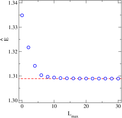
In fig. 1, we show the ground-state eigenvalue as a function of $L_{\text{max}}$. As expected, by increasing the number of states, the result becomes increasingly stable. The relative difference between the lowest eigenvalue extracted with $L_{\rm max}=28$ and with $L_{\rm max}=30$ is $\sim 10^{-6}$. The final estimate for the ground-state eigenvalue for $N_{\mbox{\scriptsize\sl f}}=3$, is therefore

$\displaystyle\hat{E}\,\overset{N_{\mbox{\tiny\rm{\sl f}}}\,=\,3}{=}\,1.309\,.$ (42)

As a further cross-check, we have discretized the Hamiltonian on a mesh grid. The two relative positions from eq. (36) live in Cartesian dimensions of extent $Na$ each, where $a$ is a lattice spacing (in units of $m_{\mbox{\tiny\rm{E}}}^{-1}$). The wave functions are then $N^{4}$-component vectors, and the Hamiltonian is an $N^{4}\times N^{4}$-matrix. For the Laplacian a 5th order discretization is adopted. We extrapolate separately $a\to 0$ with $Na$ fixed (continuum limit), and $Na\to\infty$ (infinite-volume limit), checking that the end result is independent of the ordering of these limits. Including values in the ranges $N=20...64$ and $am_{\mbox{\tiny\rm{E}}}=0.16...0.75$, we find that the results are consistent with an approximately quadratic dependence on $a$. The continuum limit yields a result compatible with eq. (42), up to all digits shown.

Inserting eq. (42) into eq. (37), leads to our NLO estimate of the baryonic screening masses,

$\displaystyle\min\{E\}\;\overset{N_{\mbox{\tiny\rm{\sl f}}}\,=\,3}{=}\;3\pi T\,\bigg{[}\,1+\bigg{(}\,\frac{1}{6\pi^{2}}+\frac{2\hat{E}}{9\pi^{2}}\,\biggr{)}g^{2}+O(g^{3})\,\bigg{]}\;\approx\;3\pi T\,\bigl{[}\,1+0.046\,g^{2}+O(g^{3})\,\bigr{]}\,.$ (43)

The NLO term represents a $\sim 4.6\%$ positive correction to the free-theory result $3\pi T$ at the electroweak scale, i.e.  $g^{2}\approx 1$ Laine:2005ai .

6 Conclusions

We have computed the NLO correction to a baryonic screening mass in thermal QCD. The computation was carried out in the framework of a dimensionally reduced effective theory, where the lowest Matsubara modes of massless quarks appear as non-relativistic fields, interacting with zero Matsubara mode gluons.

The NLO correction in eq. (43) amounts to a $\sim 4.6\%$ increase of the free-theory value $3\pi T$ at $g^{2}\approx 1$. For comparison, we note that an analogous computation for the mesonic screening masses yields a $\sim 3\%$ positive correction in the static sector Laine:2003bd , while in the non-static sector the effect is $\sim 5\%$ Brandt:2014uda . The reason for the difference lies in the form of the static potential in the corresponding Schrödinger equation. The larger correction in the baryonic and non-static mesonic sectors can be traced back to the appearance of the potential $V^{+}$ in eq. (31), which is more energetic than $V^{-}$ at short distances.

The computation of our paper was motivated by, and in turn provides motivation for, a non-perturbative determination of baryonic screening masses on the lattice Rescigno:2023tkq ; new . By comparing the two results, we can attempt to estimate the domain in which NLO computations can function as a quantitative tool for understanding the underlying physics. As discussed in more detail in ref. new , the upshot is that, assuming that the coefficients of the higher-order corrections are small, the $O(g^{2})$ term can account for $\sim 90\%$ of the difference between the non-perturbative result and the free-theory value $3\pi T$ down to temperatures of a few GeV. This suggests that baryonic observables could be more perturbative than most other quantities that have been studied so far. Of course, to consolidate this picture, it would be valuable to explicitly determine the coefficients of some higher-order corrections.

Acknowledgements

D.L. thanks the Institute for Theoretical Physics of the University of Bern for hospitality during initial stages of this work. This work was (partially) supported by ICSC – Centro Nazionale di Ricerca in High Performance Computing, Big Data and Quantum Computing, funded by European Union – NextGenerationEU. We thank CINECA for providing us with computing time on Marconi (CINECA-INFN, CINECA-Bicocca agreements).

Appendix A Dimensionally reduced effective theory

A.1 Bosonic sector

For QCD in four dimensions we adopt the conventions in appendix B of ref. DallaBrida:2020gux . At finite temperature, the gauge field can be written as

$\displaystyle A_{\mu}(x_{0},x)=g_{\mbox{\tiny\rm{E}}}\sum_{n}e^{iw_{n}x_{0}}A_{\mu,n}(x)\,,\quad x=(\mathbf{r},x_{3})\,,$ (44)

where $A_{\mu,n}(x)$ are its Matsubara modes, with $w_{n}=2\pi Tn$ and $n\in\mathbb{Z}$. The prefactor $g_{\mbox{\tiny\rm{E}}}$ on the right-hand side of eq. (44) has been chosen so as to recover the conventional perturbative normalization.

The Matsubara modes effectively acquire a mass proportional to $|w_{n}|$, and therefore the lightest degrees of freedom in the theory are the Matsubara zero modes $A_{\mu,0}(x)$. The latter are the building blocks of the dimensionally reduced effective theory. For simplicity, we denote the Matsubara zero modes by $A_{\mu}(x)$. Note that the three-dimensional field has the mass dimension $[A_{\mu}]=1/2$.

Restricting to the set of Matsubara zero modes, the gauge transformations are taken constant in $x_{0}$. In other words, the effective action has to respect three-dimensional gauge invariance. If $\Omega(x)$ is a time-independent SU(3) element, the gauge fields transform as

$\displaystyle A^{\Omega}_{i}(x)$ $\displaystyle=\Omega(x)A_{i}(x)\Omega^{\dagger}(x)+\frac{i}{g_{\mbox{\tiny\rm{E}}}}\Omega(x)\partial_{i}\Omega^{\dagger}(x)\;,$ (45)
$\displaystyle A^{\Omega}_{0}(x)$ $\displaystyle=\Omega(x)A_{0}(x)\Omega^{\dagger}(x)\,.$ (46)

The 00-component transforms in the adjoint representation of the group, and gauge invariance does not protect it from obtaining a mass term.

Given this field content, the effective action in eq. (4) is readily obtained. A discussion of higher-dimensional operators can be found in ref. Laine:2016hma .

A.2 Fermionic sector

In order to derive the effective action in eq. (6), it is useful to employ a special representation of the (Euclidean) Dirac matrices,

$\displaystyle\gamma_{0}\,=\,\begin{pmatrix}0&\mathbbm{1}\\ \mathbbm{1}&0\end{pmatrix}\,,\quad\gamma_{1}\,=\,\begin{pmatrix}\sigma_{2}&0\\ 0&-\sigma_{2}\end{pmatrix}\,,\quad\gamma_{2}\,=\,\begin{pmatrix}-\sigma_{1}&0\\ 0&\sigma_{1}\end{pmatrix}\,,\quad\gamma_{3}\,=\,\begin{pmatrix}0&-i\mathbbm{1}\\ i\mathbbm{1}&0\end{pmatrix}\,,$ (47)

where $\sigma_{i}$ are the $2\times 2$ Pauli matrices. These imply

$\displaystyle\gamma_{5}\,=\,\begin{pmatrix}-\sigma_{3}&0\\ 0&\sigma_{3}\end{pmatrix}\,,\quad C\,=i\gamma_{0}\gamma_{2}\,=\,\begin{pmatrix}0&i\sigma_{1}\\ -i\sigma_{1}&0\end{pmatrix}\quad\text{and}\quad C\gamma_{5}\,=\,\begin{pmatrix}0&\sigma_{2}\\ \sigma_{2}&0\end{pmatrix}\,,$ (48)

and where $C$ is a hermitean charge conjugation. With this representation the Dirac operator becomes

$\displaystyle\gamma_{0}\not{D}\,=\,\begin{pmatrix}D_{0}+iD_{3}\;&\;-\epsilon_{kl}D_{k}\sigma_{l}\\ \epsilon_{kl}D_{k}\sigma_{l}\;&\;D_{0}-iD_{3}\end{pmatrix}\,,$ (49)

where $k,l=1,2$ and $\epsilon_{kl}$ is the antisymmetric Levi-Civita symbol with $\epsilon_{12}=1$. Similarly to eq. (44), by using the notation of ref. Laine:2003bd , we introduce the three-dimensional two-components fields $\psi^{\uparrow}_{n}$ and $\psi^{\downarrow}_{n}$, which are eigenstates of $\gamma_{0}\gamma_{3}$. In the chosen basis, they are related to the usual four-dimensional fermionic field $\psi$ by

$\displaystyle\psi(x_{0},x)=\sqrt{T}\,\sum_{n}e^{ik_{n}x_{0}}\begin{pmatrix}\psi^{\uparrow}_{n}(x)\\ \psi^{\downarrow}_{n}(x)\end{pmatrix}\,,$ (50)

where $n$ labels the fermionic Matsubara frequencies, $k_{n}=\pi T(2n+1)$ with $n\in\mathbb{Z}$. Inserting into the action of a single massless fermion, $S_{\psi}$, we obtain 444For the notation we recall footnote 1.

$\displaystyle\begin{aligned} S_{\psi}\,=i\sum_{n}\int\!{\rm d}^{3}x\,\Big{\{}\bar{\psi}^{\uparrow}_{n}\left[k_{n}-g_{\mbox{\tiny\rm{E}}}A_{0}+D_{3}\right]&\psi^{\uparrow}_{n}+\bar{\psi}^{\downarrow}_{n}\left[k_{n}-g_{\mbox{\tiny\rm{E}}}A_{0}-D_{3}\right]\psi^{\downarrow}_{n}\\ &-i\bar{\psi}^{\downarrow}_{n}\epsilon_{kl}D_{k}\sigma_{l}\psi^{\uparrow}_{n}+i\bar{\psi}^{\uparrow}_{n}\epsilon_{kl}D_{k}\sigma_{l}\psi^{\downarrow}_{n}\Big{\}}\,.\end{aligned}$ (51)

For a generic interpolating operator $O(y)$, the corresponding equations of motion are

$\displaystyle\begin{aligned} i&\expectationvalue{\Bigl{\{}\,\left[k_{n}-g_{\mbox{\tiny\rm{E}}}A_{0}+D_{3}\right]\psi^{\uparrow}_{n}+i\epsilon_{kl}D_{k}\sigma_{l}\psi^{\downarrow}_{n}\,\Bigr{\}}(x)\,O(y)}=\expectationvalue{\frac{\delta O(y)}{\delta\bar{\psi}^{\uparrow}_{n}(x)}}\,,\\[7.11317pt] i&\expectationvalue{\Bigl{\{}\,\left[k_{n}-g_{\mbox{\tiny\rm{E}}}A_{0}-D_{3}\right]\psi^{\downarrow}_{n}-i\epsilon_{kl}D_{k}\sigma_{l}\psi^{\uparrow}_{n}\,\Bigr{\}}(x)\,O(y)}=\expectationvalue{\frac{\delta O(y)}{\delta\bar{\psi}^{\downarrow}_{n}(x)}}\,,\end{aligned}$ (52)

and analogously if we vary with respect to ${\psi}^{\uparrow}_{n}$ and ${\psi}^{\downarrow}_{n}$.

By inspecting the free limit, it is clear that for each Matsubara mode there is a mass term equal to $k_{n}$. As a consequence, the lightest modes are in the sectors $n=0$ and $n=-1$. Considering propagation in the positive-$x_{3}$ direction and looking at the relative sign between the mass term and the kinetic term, the light modes are $\psi^{\uparrow}_{0}$ and $\psi^{\downarrow}_{-1}$. By solving the equations of motion for $\psi^{\uparrow}_{0}$ and $\psi^{\downarrow}_{-1}$ at $O(g_{\mbox{\tiny\rm{E}}}^{2})$, we obtain the equations of motion in eqs. (8) and (9), where we have dubbed $\chi=\psi^{\uparrow}_{0}$ and $\phi=\psi^{\downarrow}_{-1}$, respectively.

field/operator power counting
$\chi,\phi$ $m_{\mbox{\tiny\rm{E}}}$
$\partial_{3}\sim\Delta E$ $g^{2}_{\mbox{\tiny\rm{E}}}$
$\nabla_{\mathbf{r}}^{2}=\nabla_{\perp}^{2}\sim\mathbf{p}^{2}$ $m_{\mbox{\tiny\rm{E}}}^{2}$
${\rm d}^{3}x$ $g_{\mbox{\tiny\rm{E}}}^{-2}m_{\mbox{\tiny\rm{E}}}^{-2}$
Table 1: Power counting for the fermionic fields in eq. (6) and for their variation in longitudinal ($x_{3}$) and transverse ($\mathbf{r}=x_{\perp}$) directions.

In order to determine NLO corrections to hadronic correlation functions, it is helpful to establish the power counting deriving from the three-dimensional action. The relevant scales of the system are $m_{\mbox{\tiny\rm{E}}}$, $g_{\mbox{\tiny\rm{E}}}^{2}$ and the thermal quark mass $k_{0}\approx M$, originating from the lowest fermionic Matsubara frequency. The power-counting rules are given in table 1. As a consequence, the action in eq. (6) is obtained by taking into account spinor fields in the lowest Matsubara sector, including terms up to $O(g_{\mbox{\tiny\rm{E}}}^{0})$, and labelling, at variance with appendix B of ref. DallaBrida:2020gux , the $N_{\mbox{\scriptsize\sl f}}=3$ flavours as f$\;=u,d,s$.

Appendix B Fermionic propagators in the effective theory

In coordinate space, by making explicit the source and the sink locations, the propagator from eq. (13) becomes

$\displaystyle S^{(0)}_{\chi}(\mathbf{x},x_{3};\mathbf{y},y_{3})=\frac{-i\theta(x_{3}-y_{3})T\mathbbm{1}}{2(x_{3}-y_{3})}\exp\left[-M(x_{3}-y_{3})-\frac{\pi T\left(\mathbf{x}-\mathbf{y}\right)^{2}}{2\left(x_{3}-y_{3}\right)}\right]\,,$ (53)

and similarly but with opposite sign for $\phi$. At the next order, from eq. (11), the propagator for $\chi$ reads

$\displaystyle\begin{aligned} S^{(1)}_{\chi}(\mathbf{x},x_{3};\mathbf{y},y_{3})\;=\;i\int\!{\rm d}z_{3}\!\int\!{\rm d}^{2}\mathbf{z}\,S^{(0)}_{\chi}&(\mathbf{x},x_{3};\mathbf{z},z_{3})\left[iA_{3}+A_{0}\right](\mathbf{z},z_{3})S^{(0)}_{\chi}(\mathbf{z},z_{3};\mathbf{y},y_{3})\,,\end{aligned}$ (54)

implying that $\chi$ propagates freely from the source to the position $(\mathbf{z},z_{3})$, where it emits a gluon, and then again freely propagates up to the sink position. By inserting eq. (53) into eq. (54) and taking $(\mathbf{y},y_{3})=(\mathbf{0},0)$, the result can be rewritten as

$\displaystyle\begin{aligned} S^{(1)}_{\chi}(\mathbf{x},x_{3};\mathbf{0},0)\;&=\;S^{(0)}_{\chi}(\mathbf{x},x_{3};\mathbf{0},0)\int_{0}^{x_{3}}\!{\rm d}z_{3}\,\int\!{\rm d}^{2}\mathbf{z}\,\frac{x_{3}T}{2(x_{3}-z_{3})z_{3}}\\[3.55658pt] &\times\exp\left[-\frac{1}{2}\frac{\pi T}{\left(x_{3}-z_{3}\right)}\frac{x_{3}}{z_{3}}\left(\mathbf{z}-\frac{z_{3}}{x_{3}}\mathbf{x}\right)^{2}\right]\left[iA_{3}+A_{0}\right](\mathbf{z},z_{3})\,.\end{aligned}$ (55)

From table 1 we see that the prefactor of the quadratic dependence is parametrically of order $\pi Tx_{3}/[(x_{3}-z_{3})z_{3}]\sim\pi Tg_{\mbox{\tiny\rm{E}}}^{2}$, implying that fermions probe the variation of gauge fields at distances $|\mathbf{z}-z_{3}\mathbf{x}/x_{3}|\sim 1/(gT)\sim 1/m_{\mbox{\tiny\rm{E}}}$. For the static potential, we need the $x_{3}\to\infty$ limit, and then only the position of the gauge field at $z_{3}\sim x_{3}$ matters. Then the prefactor is large, and we may evaluate the integral in the saddle point approximation, yielding

$\displaystyle\begin{aligned} S^{(1)}_{\chi}(\mathbf{x},x_{3};\mathbf{0},0)\;\simeq\;S^{(0)}_{\chi}(\mathbf{x},x_{3};\mathbf{0},0)\,\int_{0}^{x_{3}}\!{\rm d}z_{3}\,\left[iA_{3}+A_{0}\right]\left(\frac{z_{3}}{x_{3}}\mathbf{x},z_{3}\right)\,,\end{aligned}$ (56)

justifying eq. (16).

Appendix C Evaluation of the static potential

We show here details for the manipulation of eq. (4.3). The free-theory gauge field propagator reads

$\displaystyle\bigl{\langle}\,A^{a}_{\mu}(x)A^{b}_{\nu}(0)\,\bigr{\rangle}_{0}=\delta^{ab}\Delta_{\mu\nu}(x)\,,$ (57)

where $\mu,\nu=0,\dots,3$, $a,b=1,\dots,8$ and, in Feynman gauge,

$$\Delta_{\mu\nu}(x)\;=\;\int\!\frac{{\rm d}^{3}p}{(2\pi)^{3}}\,e^{ip\cdot x}\,\biggl{[}\,\frac{\delta_{\mu 0}\delta_{\nu 0}}{p^{2}+m_{\mbox{\tiny\rm{E}}}^{2}}\,+\,\frac{\delta_{\mu i}\delta_{\nu i}}{p^{2}+\lambda^{2}}\,\biggr{]}\;,\quad p=(\mathbf{p},p_{3})\,.$$ (58)

The Debye mass $m_{\mbox{\tiny\rm{E}}}$ is given in eq. (5), and $\lambda$ is an auxiliary mass parameter, used as an IR regulator. The Wick contractions following from eq. (4.3) lead to the colour algebra

$$\epsilon^{abc}\epsilon^{gfe}(T^{d}T^{d})^{ag}\delta^{bf}\delta^{ce}=8\;,\quad\epsilon^{abc}\epsilon^{gfe}(T^{d})^{ag}(T^{d})^{bf}\delta^{ce}=-4\,,$$ (59)

where $T^{d}$ are Hermitean generators of SU(3), normalized as $\tr(T^{c}T^{d})=\delta^{cd}/2$. Subsequently, we are left over with the time-integrals

$\displaystyle{\cal V}^{\pm}(\textbf{r}_{1},\textbf{r}_{2},x_{3})\equiv-\int_{0}^{x_{3}}\!{\rm d}z_{3}\,\Big{[}\Delta_{33}\Bigl{(}\,\textbf{r}_{1}-\textbf{r}_{2}+\frac{z_{3}}{x_{3}}\textbf{r}_{2},z_{3}\,\Bigr{)}\mp\Delta_{00}\Bigl{(}\,\textbf{r}_{1}-\textbf{r}_{2}+\frac{z_{3}}{x_{3}}\textbf{r}_{2},z_{3}\,\Bigr{)}\Big{]}\,.$ (60)

The propagators are written in a Fourier representation, like in eq. (58). In the limit $x_{3}\rightarrow\infty$, noting that

$$\lim_{\delta\to 0^{+}}\lim_{x_{3}\to\infty}\int_{0}^{x_{3}}\!{\rm d}z_{3}\,e^{\bigl{[}i(\frac{\textbf{p}\cdot\textbf{r}}{x_{3}}+p_{3})-\delta\bigr{]}z_{3}}\;=\;\lim_{\delta\to 0^{+}}\lim_{x_{3}\to\infty}\frac{i}{\frac{\textbf{p}\cdot\textbf{r}}{x_{3}}+p_{3}+i\delta}\;=\;\mathbbm{P}\biggl{(}\frac{i}{p_{3}}\biggr{)}+\pi\delta(p_{3})\;,$$ (61)

where $\mathbbm{P}$ denotes a principal value, and pulling the time integral inside the Fourier representation, the Fourier transform becomes

$$\int_{\textbf{p}}\int_{-\infty}^{\infty}\!\frac{{\rm d}p_{3}}{2\pi}\int_{0}^{x_{3}}\!{\rm d}z_{3}\,\frac{e^{i\textbf{p}\cdot(\textbf{r}_{1}-\textbf{r}_{2}+\frac{z_{3}}{x_{3}}\textbf{r}_{2})+ip_{3}z_{3}}}{f(\textbf{p}^{2},p_{3}^{2})}\stackrel{{\scriptstyle x_{3}\to\infty}}{{\longrightarrow}}\frac{1}{2}\int_{\textbf{p}}\frac{e^{i\textbf{p}\cdot(\textbf{r}_{1}-\textbf{r}_{2})}}{f(\textbf{p}^{2},0)}\;.$$ (62)

Carrying out the two-dimensional momentum integral, the potential reads

$\displaystyle\lim_{x_{3}\rightarrow\infty}{\cal V}^{\pm}(\textbf{r}_{1},\textbf{r}_{2},x_{3})=\frac{1}{4\pi}\left[\ln\left(\frac{\lambda\,r_{12}}{2}\right)+\gamma_{\mbox{\tiny\rm{E}}}\pm K_{0}(m_{\mbox{\tiny\rm{E}}}r_{12})\right]\,,$ (63)

where $r_{12}\equiv|\textbf{r}_{1}-\textbf{r}_{2}|$, $\gamma_{\mbox{\tiny\rm{E}}}$ is the Euler-Mascheroni constant, and $K_{0}$ a modified Bessel function. The combinations that appear in eq. (27) are defined as

$\displaystyle V^{\pm}(r_{12})\;\equiv\;\frac{4g^{2}_{\mbox{\tiny\rm{E}}}}{3}\lim_{\lambda\rightarrow 0}\lim_{x_{3}\rightarrow\infty}\bigl{[}{\cal V}^{\pm}(\textbf{r}_{1},\textbf{r}_{2},x_{3})+{\cal V}^{\pm}(\textbf{r}_{2},\textbf{r}_{1},x_{3})-{\cal V}^{+}(\textbf{r}_{1},\textbf{r}_{1},x_{3})-{\cal V}^{+}(\textbf{r}_{2},\textbf{r}_{2},x_{3})\bigr{]}\,.$ (64)

By using the expansion of $K_{0}(x)$ for small $x$, it is straightforward to show that

$$\lim_{x_{3}\rightarrow\infty}{\cal V}^{+}(\textbf{r}_{1},\textbf{r}_{1},x_{3})=\frac{1}{4\pi}\ln\left(\frac{\lambda}{m_{\mbox{\tiny\rm{E}}}}\right)\,.$$ (65)

This then leads to the explicit expressions for $V^{\pm}(r)$ reported in eq. (29).

Appendix D Two-dimensional hyperspherical harmonics

Let us consider a system of three particles of mass $m$ which are constrained to move in a two-dimensional plane. We assume those particles to interact through mutual two-body potentials which depend only on relative separations. The Schrödinger equation for such a system is

$\displaystyle\left[-\frac{1}{2m}\sum_{i=1}^{3}\nabla_{\mathbf{r}_{i}}^{2}+\sum_{j>i}^{3}V(r_{ij})\right]\psi(\mathbf{r}_{1},\mathbf{r}_{2},\mathbf{r}_{3})\,=\,E\,\psi(\mathbf{r}_{1},\mathbf{r}_{2},\mathbf{r}_{3})\,,$ (66)

where $r_{ij}\equiv|\mathbf{r}_{i}-\mathbf{r}_{j}|$. By performing the change of variables in eq. (33), the Laplace operator can be written as

$\displaystyle\frac{1}{2}\Bigl{[}\nabla_{{\mathbf{r}}_{1}}^{2}+\nabla_{{\mathbf{r}}_{2}}^{2}+\nabla_{{\mathbf{r}}_{3}}^{2}\Bigr{]}\,=\,\frac{\nabla_{{\mathbf{R}}}^{2}}{6}+\nabla_{{{\bm{\xi}}}_{1}}^{2}+\nabla_{{{\bm{\xi}}}_{2}}^{2}\,,$ (67)

where ${\mathbf{R}}$ is the center-of-mass coordinate. In such a way, the kinetic energy can be separated into center-of-mass and relative motions. The Schrödinger equation for the relative motion can be written in terms of the new coordinates as

$\displaystyle\left\{-\frac{1}{m}\left(\nabla_{{{\bm{\xi}}_{1}}}^{2}+\nabla_{{{\bm{\xi}}}_{2}}^{2}\right)+{V}\left({{\bm{\xi}}_{1}},{{\bm{\xi}}_{2}}\right)\right\}{\Psi}\left({{\bm{\xi}}_{1}},{{\bm{\xi}}_{2}}\right)\,=\,E\,\Psi\left({{\bm{\xi}}_{1}},{{\bm{\xi}}_{2}}\right)\,.$ (68)

By going to polar coordinates, i.e.

$\displaystyle\begin{cases}{\xi}_{1}^{(1)}\,=\,{\xi}_{1}\cos\theta_{1}\\ {\xi}_{1}^{(2)}\,=\,{\xi}_{1}\sin\theta_{1}\end{cases}\qquad\begin{cases}{\xi}_{2}^{(1)}\,=\,{\xi}_{2}\cos\theta_{2}\\ {\xi}_{2}^{(2)}\,=\,{\xi}_{2}\sin\theta_{2}\end{cases}\,,$ (69)

where ${\xi}_{i}$ refers to the absolute value of the 2-vector ${{\bm{\xi}}}_{i}$ and the superscript $(j)$ refers to the components in the two-dimensional plane, the Laplace operator can be expressed as

$\displaystyle\nabla^{2}_{{{\bm{\xi}}}_{1}}+\nabla^{2}_{{{\bm{\xi}}}_{2}}\,=\,\frac{\partial^{2}}{\partial{\xi}_{1}^{2}}+\frac{1}{{\xi}_{1}}\frac{\partial}{\partial{\xi}_{1}}+\frac{1}{{\xi}_{1}^{2}}\frac{\partial^{2}}{\partial\theta_{1}^{2}}\,+\,\frac{\partial^{2}}{\partial{\xi}_{2}^{2}}+\frac{1}{{\xi}_{2}}\frac{\partial}{\partial{\xi}_{2}}+\frac{1}{{\xi}_{2}^{2}}\frac{\partial^{2}}{\partial\theta_{2}^{2}}\,.$ (70)

Both for ${\xi}_{1}$ and ${\xi}_{2}$ the angular differential operator corresponds to the square of the two-dimensional quantum-mechanical angular momentum operator,

$\displaystyle\mathbf{L}_{i}\,\equiv\,(-i)\frac{\partial}{\partial\theta_{i}}\qquad\textrm{for}\quad i=1,2\,.$ (71)

We also note that the scalar products following from eqs. (33) and  (34) read

$$r_{12}=\frac{\sqrt{\xi_{1}^{2}+3\xi_{2}^{2}+2\sqrt{3}{{\bm{\xi}}}_{1}\cdot{{\bm{\xi}}}_{2}}}{2}\;,\quad r_{13}=\xi_{1}\;,\quad r_{23}=\frac{\sqrt{\xi_{1}^{2}+3\xi_{2}^{2}-2\sqrt{3}{{\bm{\xi}}}_{1}\cdot{{\bm{\xi}}}_{2}}}{2}\,,$$ (72)

where ${{\bm{\xi}}}_{1}\cdot{{\bm{\xi}}}_{2}=\xi_{1}\xi_{2}\cos(\theta_{1}-\theta_{2})$.

So far, our coordinates comprise two radial extension ${\xi}_{i}$ and two angles $\theta_{i}$. The idea underlying the hyperspherical harmonics method is to write the system, by a suitable change of variables, in terms of one radial and three angular variables. This is achieved by going to the so-called hyperspherical coordinates,

$\displaystyle\begin{cases}{\xi}_{1}\,=\,\xi\sin\phi\\ {\xi}_{2}\,=\,\xi\cos\phi\end{cases}\,,$ (73)

where $\xi$ is called the hyper-radius and the angular variable $\phi$ describes the relative length between the two vectors ${{\bm{\xi}}}_{1}$ and ${{\bm{\xi}}}_{2}$, i.e.  $\phi\in[0,\pi/2]$. Together with $\theta_{1}$ and $\theta_{2}$, $\phi$ forms a set of so-called hyper-angles $\Omega_{4}\equiv\left\{\theta_{1},\theta_{2},\phi\right\}$. With this change of variables, the Laplace operator in eq. (70) becomes

$\displaystyle\nabla^{2}_{\xi}\,\equiv\,\nabla^{2}_{{{\bm{\xi}}}_{1}}+\nabla^{2}_{{{\bm{\xi}}}_{2}}\,=\,\frac{\partial^{2}}{\partial\xi^{2}}+\frac{3}{\xi}\frac{\partial}{\partial\xi}-\frac{\mathcal{L}^{2}\left(\Omega_{4}\right)}{\xi^{2}}\,,$ (74)

where we introduced the hyperangular momentum operator

$\displaystyle\mathcal{L}^{2}\left(\Omega_{4}\right)\;\equiv\;-\left[\frac{\partial^{2}}{\partial^{2}\phi}+2\cot{2\phi}\,\frac{\partial}{\partial\phi}-\frac{\mathbf{L}^{2}_{1}}{\sin^{2}\phi}-\frac{\mathbf{L}^{2}_{2}}{\cos^{2}\phi}\right]\,.$ (75)

In complete analogy with the angular momentum operator, we can define the eigenvalues and eigenstates of the hyperangular momentum operator by assuming that $\xi^{L}\mathcal{Y}\left(\Omega_{4}\right)$ is a harmonic function. This leads to

$\displaystyle\mathcal{L}^{2}\left(\Omega_{4}\right)\mathcal{Y}\left(\Omega_{4}\right)\,=\,L\left(L+2\right)\mathcal{Y}\left(\Omega_{4}\right)\,,$ (76)

where $L$, in analogy with the angular momentum quantum number, is called the grand orbital quantum number. Given the form of the operator in eq. (75), the corresponding eigenvectors can be written as

$\displaystyle\mathcal{Y}_{L}\left(\Omega_{4}\right)\,=\,\mathcal{P}_{L}^{l_{1}l_{2}}\left(\phi\right)Y_{l_{1}}\left(\theta_{1}\right)Y_{l_{2}}\left(\theta_{2}\right)\,,$ (77)

where $Y_{l_{i}}(\theta)$ are the eigenvectors of the $\mathbf{L}_{i}$ operators, i.e.

$\displaystyle Y_{l_{i}}\left(\theta_{i}\right)\,=\,\frac{e^{il_{i}\theta_{i}}}{\sqrt{2\pi}}\qquad\text{with}\qquad l_{i}\,\in\,\mathbb{Z}\,.$ (78)

By looking for a solution of the type

$\displaystyle\mathcal{P}_{L}^{l_{1}l_{2}}\left(\phi\right)\,=\,\mathcal{N}^{l_{1}l_{2}}_{L}\left(\sin\phi\right)^{|l_{1}|}\left(\cos\phi\right)^{|l_{2}|}g\left(\cos 2\phi\right)\,,$ (79)

and by performing the change of variables $x=\cos 2\phi$, the differential equation in eq. (76) can be written as

$\displaystyle\left(1-x^{2}\right)\frac{\partial^{2}g}{\partial x^{2}}\,+\,\big{[}|l_{2}|-|l_{1}|$ $\displaystyle-(|l_{1}|+|l_{2}|+2)\,x\,\big{]}\frac{\partial g}{\partial x}+\,\left(n+|l_{1}|+|l_{2}|+1\right)n\,g\,=\,0\,,$ (80)

where $n$ is related to the quantum numbers $l_{1},l_{2}$ and $L$ by

$\displaystyle L\,=\,2n+|l_{1}|+|l_{2}|\qquad\text{with}\qquad n\in\mathbb{N}\,.$ (81)

Equation (80) has analytical solutions in terms of Jacobi polynomials,

$\displaystyle g(x)\,=\,P_{n}^{l_{1}l_{2}}(x)\,=\,\frac{\left(1+|l_{1}|\right)_{n}}{n!}\,\leftidx{{}_{2}}{F}{{}_{1}}\left(-n,n+|l_{1}|+|l_{2}|+1;|l_{1}|+1;\frac{1-x}{2}\right)\,$

where $(\cdot)_{n}$ is the Pochhammer symbol and $\leftidx{{}_{2}}{F}{{}_{1}}$ is the hypergeometric function. These polynomials are orthogonal in the interval $[-1,1]$ with respect to the weight function $\left(1-x\right)^{|l_{1}|}\left(1+x\right)^{|l_{2}|}$, and their normalization constant is given by

$\displaystyle\int_{-1}^{1}\!{\rm d}x\,P_{n}^{l_{1}l_{2}}(x)P_{n^{\prime}}^{l_{1}l_{2}}(x)$ $\displaystyle\left(1-x\right)^{|l_{1}|}\left(1+x\right)^{|l_{2}|}$ (82)
$\displaystyle=\,\frac{\delta_{n,n^{\prime}}\,2^{|l_{1}|+|l_{2}|+1}}{2n+|l_{1}|+|l_{2}|+1}\frac{\Gamma\left(n+|l_{1}|+1\right)\Gamma\left(n+|l_{2}|+1\right)}{\Gamma\left(n+1\right)\Gamma\left(n+|l_{1}|+|l_{2}|+1\right)}\;,$

where $\Gamma$ is the Euler gamma function.

By inserting the solution into eq. (79), and taking into account the volume element for the angular variables, $\mathop{}\!\mathrm{d}\Omega_{4}\,\equiv\,\sin\phi\cos\phi\,\mathop{}\!\mathrm{d}\phi\,\mathop{}\!\mathrm{d}\theta_{1}\,\mathop{}\!\mathrm{d}\theta_{2}$, the normalization of the eigenvectors in eq. (79) is obtained by integrating over the hyperangle $\phi$,

$\displaystyle\bigl{(}\mathcal{N}_{L}^{l_{1}l_{2}}\bigr{)}^{2}\int_{0}^{\frac{\pi}{2}}\!{\rm d}\phi\,\left(\sin\phi\right)^{2|l_{1}|+1}\left(\cos\phi\right)^{2|l_{2}|+1}P_{n}^{l_{1}l_{2}}(\cos 2\phi)P_{n^{\prime}}^{l_{1}l_{2}}(\cos 2\phi)\,=\,\delta_{n,n^{\prime}}\,.$ (83)

This determines the normalization constant,

$\displaystyle\mathcal{N}_{L}^{l_{1}l_{2}}\,=\,\left[\frac{2\left(L+1\right)\Gamma\left(n+1\right)\Gamma\left(L-n+1\right)}{\Gamma\left(n+|l_{1}|+1\right)\Gamma\left(n+|l_{2}|+1\right)}\right]^{\frac{1}{2}}\,.$ (84)

As a consequence, the hyperspherical harmonics ${\cal Y}_{L}$ satisfy the orthonormality relation

$\displaystyle\int\!{\rm d}\Omega_{4}\,\mathcal{Y}_{L}^{*}\left(\Omega_{4}\right)\mathcal{Y}_{L^{\prime}}\left(\Omega_{4}\right)\,=\,\delta_{l_{1},l_{1}^{\prime}}\delta_{l_{2},l_{2}^{\prime}}\delta_{n,n^{\prime}}\,.$ (85)

The hyperspherical harmonics form a complete set on the surface described by the angles $\left\{\phi,\theta_{1},\theta_{2}\right\}$ at fixed $\xi$. As a consequence, the wave functions appearing in eq. (68) can be expanded as

$\displaystyle\Psi\left({{\bm{\xi}}_{1}},{{\bm{\xi}}_{2}}\right)\,=\,\sum_{\{L\}}\Phi_{\{L\}}\left(\xi\right)\mathcal{Y}_{\{L\}}\left(\Omega_{4}\right)\,,$ (86)

where $\{L\}$ refers to any particular combination of quantum numbers which leads to $L=2n+|l_{1}|+|l_{2}|$, and the expansion coefficients $\Phi_{\{L\}}$ encode the hyper-radial dependence of the wave function. We can get rid of the first derivative appearing in eq. (74) by writing the expansion coefficient as $\Phi_{\{L\}}\left(\xi\right)=u_{\{L\}}\left(\xi\right)/\xi^{3/2}$. Therefore, by using eq. (76), the Schrödinger equation can be written as

$\displaystyle\sum_{\{L^{\prime}\}}\left\{-\frac{1}{m}\left[\frac{\partial^{2}}{\partial\xi^{2}}-\frac{3}{4\xi^{2}}-\frac{L^{\prime}\left(L^{\prime}+2\right)}{\xi^{2}}\right]+V\left(\xi,\Omega_{4}\right)-E\right\}u_{\{L^{\prime}\}}\left(\xi\right)\mathcal{Y}_{\{L^{\prime}\}}\left(\Omega_{4}\right)\,=\,0\,.$ (87)

By multiplying on the left by $\mathcal{Y}^{*}_{\{L\}}\left(\Omega_{4}\right)$ and integrating over $\Omega_{4}$, the orthogonality relation for the hyperspherical harmonics, eq. (85), leads to the final form

$\displaystyle\left\{-\frac{1}{m}\left[\frac{\partial^{2}}{\partial\xi^{2}}-\frac{3}{4\xi^{2}}-\frac{L\left(L+2\right)}{\xi^{2}}\right]\,-\,E\right\}u_{\{L\}}\left(\xi\right)\,+\,\sum_{\{L^{\prime}\}}\mathcal{V}_{\{L,L^{\prime}\}}\left(\xi\right)\,u_{\{L^{\prime}\}}\left(\xi\right)=0\,,$ (88)

where

$\displaystyle\mathcal{V}_{\{L,L^{\prime}\}}\left(\xi\right)\,=\,\int\!{\rm d}\,\Omega_{4}\,\mathcal{Y}_{\{L\}}^{*}\left(\Omega_{4}\right){V}\left(\xi,\Omega_{4}\right)\mathcal{Y}_{\{L^{\prime}\}}(\Omega_{4})$ (89)

are the matrix elements computed in the basis of the hyperspherical harmonics.

In this way, the Schrödinger equation has been reduced to a set of coupled one-dimensional differential equations which are easier to solve numerically. With this procedure, the bulk of the calculation is given by the computation of the matrix elements by properly truncating the basis up to a certain value $L_{\text{max}}$. The number of states to be included can be reduced by scrutinizing the physics of the problem of interest. Given that our potential $V$ only depends on $\theta_{1}-\theta_{2}$ (cf. eq. (72)), the total angular momentum in the transverse plane, with its eigenvalue $l_{1}+l_{2}$, commutes with the Hamiltonian and represents a conserved quantity. In order to extract the energy of the ground state, it is then sufficient to consider the smallest value of the total angular momentum, i.e. set $l_{2}=-l_{1}$ in eq. (81). This implies that the grand orbital quantum number is restricted to even values only,

$\displaystyle L=2\left(n+|l_{1}|\right)\,.$ (90)

Furthermore, given that the potential is invariant under $\theta_{1}\to\theta_{1}+\pi$, we can restrict to wave functions symmetric under this “parity”, and choose $l_{1}$ even. In general, any fixed $L$ describes a set $\{L\}$ of various $n$ and $l_{1}$.

References