Quantum Circuit Optimisation and MBQC Scheduling with a Pauli Tracking Library

Abstract

We present a software library for the commutation of Pauli operators through quantum Clifford circuits, which is called Pauli tracking. Tracking Pauli operators allows one to reduce the number of Pauli gates that must be executed on quantum hardware. This is relevant for measurement-based quantum computing and for error-corrected circuits that are implemented through Clifford circuits. Furthermore, we investigate the problem of qubit scheduling in measurement-based quantum computing and how Pauli tracking can be used to capture the constraints on the order of measurements.

1 Introduction

Realising fault-tolerant quantum gates and qubits is costly in terms of space, time and energy. It is crucial to reduce the number of gates as much as possible. This optimisation can be tackled on multiple levels, e.g., optimising the quantum algorithm on the logical circuit level, similar to how classical compilers optimise classical algorithms, or trying to develop more efficient error correcting codes.

Another problem that appears in the context of measurement-based quantum computation (MBQC) [1, 2], but partially also in quantum error correction (QEC), are dynamic corrections that are induced into the computation because of the nondeterminism of the measurements. For an efficient computation, these corrections have to be actively accounted for, and cannot be ignored through post-selection. They are also an essential piece of information for qubit scheduling, i.e., re-using qubits after they have been measured, as it defines an order on the measurements, which we shall explain in more detail.

In this paper, we shall focus on the classical tracking of Pauli operators through a quantum circuit, called Pauli tracking [3, 4, 5, 6], which deals with the second problem introduced above and (partially) with the first problem. Pauli tracking, we shall explain it below, is an optimisation done on the software level that directly reduces the number of Pauli gates that must be executed on the quantum hardware. Furthermore, it can capture the information of dynamic Pauli correction induced by measurements. Pauli tracking is applicable whenever the quantum circuit comprised of Clifford gates (and arbitrary measurements), as for example, in MBQC, but also in the context of QEC, e.g., the surface code [7, 8]. The QEC codes themselves are often Clifford circuits on the level of the (uncorrected) physical qubit; but also on the logical fault-tolerant level, the non-Clifford gates are usually realised via injection of certain “magic” states or specific measurements with the help of additional ancilla qubits that are entangled using only Clifford gates (cf. Fig. 1) [9, 10, 8]. Therefore, Pauli tracking can be applied on both levels in QEC, i.e., on the physical level and the logical level, which gives it together with MBQC a wide range of applications.

Let us now sketch out what we mean with Pauli tracking and how it works; it is based on the mathematical foundations discussed in [11, 12, 13]. The Clifford group is the normaliser of the Pauli group, meaning that conjugating the Pauli group with Clifford operators preserves the Pauli group. This implies that Pauli operators can be classically efficiently, i.e., without exponential costs, commuted with Clifford operators. A central implication of that characteristic is the Gottesman-Knill theorem [14], which states that circuits consisting only of Clifford gates can be efficiently simulated with a classical computer via a stabiliser simulator, e.g., [15]. For universal quantum computation, however, the Clifford group is not sufficient, i.e., we need additional non-Clifford gates. In this case, stabiliser simulators are not efficient anymore, however, for certain realisations of quantum computers, we can still make use of the fact that the Pauli group is preserved under conjugation of Clifford operators. For example, in MBQC or in the context of QEC, where the circuits only consist of Clifford gates and measurements, it is possible to traverse the Pauli operators through the circuit by commuting them with the Clifford gates until a measurement is reached and then account for the Pauli operators through post-processing or adaption of the of the measurement (cf. Fig. 1 (c)). This effectively reduces the number of Pauli gates that have to be executed on the quantum hardware to the number of qubits or less.

In Sec. 2, we present a library that can be used to perform the Pauli tracking [16]. It is a low-level library, natively written in Rust, with a Python wrapper and a partial C interface. The library is designed to be dynamically used when compiling, or executing quantum circuits and supports various generic data structures for different use cases. See Sec. 5 for how to access the library.

Now when teleporting non-Clifford gates in the context of QEC, or in general any gate as in MBQC, the non-determinism of the according measurements usually introduces Pauli corrections (or in general Clifford corrections) conditioned on the measurement outcomes, as for example, depicted in Fig. 1. These corrections effectively define a strict partial time order for the execution of the circuit, because of their non-determinism in general. The tracking of the Pauli corrections through the circuit directly captures this order (except of the order induced by possible Clifford corrections, however, they can also be deferred with an additional teleportation; cf. Fig. 1 (c)) and reduces it to the measurements. Analysing this information, in connection with entanglement structure of the circuit or graph state, gives knowledge about how the computation can be optimised in space and in time, i.e., what is the minimal number of required qubits (fully space optimised), what is the minimal number of steps of parallel measurements (fully time optimised), or in general, given a fixed number of qubits, how many steps of parallel measurements are required. Furthermore, capturing this time order and the corrections is necessary for certain MBQC compilation strategies and frameworks, e.g., Refs. [17, 18], where a logical circuit is transformed into a logical graph state (using teleportation techniques and stabilizer simulations) and the captured time order defines how the graph state is consumed.

In Sec. 3, we shall focus on this problem. More specifically, we define the scheduling problem for MBQC, which may also be applied in the context of QEC circuits locally at the parts where non-Clifford gates are teleported, and tackle it detached from the underlying quantum circuit on the logical level (i.e., we do not consider the quantum hardware). The problem will be defined in a way that is applicable to MBQC protocols like the Raussendorf cluster [1], but also other protocols that involve more complex graph states, e.g., Refs. [17, 18], or in general, whenever the entanglement structure of the circuit can be described with a graph and teleportation techniques are used for non-Clifford gates. However, note that the algorithm for the space-time optimisation that we provide is only scalable to a certain degree due to the hardness of the problem (the problem is related to finding the pathwidth of a graph [19]). This can be resolved if the input can be split into smaller problems (e.g., one might be able to serially split the circuit [18]), but if the goal is to optimise larger inputs, more optimised algorithms may be required. However, as a preview, note that finding a time-optimal solution is independent of the underlining graph, and therefore not restricted to pure MBQC, and can be directly calculated from the Pauli tracking in polynomial time.

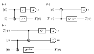
Figure 1: Example of $T$ gate teleportation; these are typical protocols in MBQC but also especially in QEC where the ancilla states, $T\left\lvert+\right\rangle$, are prepared in a distillation process [20]. The input state $\left\lvert\psi\right\rangle$ is teleported to the output state $T\left\lvert\psi\right\rangle$. (a) The $T$ teleportation is achieved with a “magic” measurement $TXT^{\dagger}$. This introduces a Pauli correction $Z$ on the output qubit depending on the measurement result. The correction can be tracked as a Pauli frame through a subsequent Clifford+measurement circuit, unblocking the execution until a measurement is reached for which the Pauli frame defines a non-trivial correction. (b) Implementation of the $T$ teleportation through injection of a “magic” state $T\left\lvert+\right\rangle$. This protocol introduces a potential $S$ (phase gate) correction on the output qubit. Since this correction cannot be tracked through the subsequent circuit, it is blocking, i.e., the execution on the output qubit has to wait until the measurement result $s$ is known. (c) Implementing the $T$ teleportation with a magic state injection, however, without blocking the execution. This circuit is constructed by taking circuit (a) and then implement the $T$ gate there with circuit (b). This way the blocking $S$ correction is removed from the output qubit. The $Z^{m}$ correction on the output qubit can be obtained through Pauli tracking: commute the $X$ correction in circuit (b) through the $S$ correction, turning it into a $ZX\propto Y$ correction; the $X$ part does not matter for the following $X$ measurement and can be completely removed; the $Z$ part, however, flips the measurement result $s$, which can be accounted for by moving the $Z$ correction onto the output qubit as a $Z$ correction (since $s$ induces a $Z$ correction). All of these three operations, commute, remove, and move, are supported in our Pauli tracking library.

2 The Pauli Tracking Library

In Section 1, we already sketched out the basic idea. Here, we shall focus on a mathematical description which directly represents how the library is implemented. Afterwards, we discuss some features of the library.

2.1 Mathematical Formulation

The Pauli operators, $X\mathchar 44\relax Y\mathchar 44\relax Z\in\mathrm{U}\left\lparen\mathbb{C}^{2}\right\rparen$, where $\mathrm{U}$ denotes the unitary group, are defined as

$$X\coloneq\begin{pmatrix}0&1\\ 1&0\end{pmatrix}\quad Y\coloneq\begin{pmatrix}0&-i\\ i&0\end{pmatrix}\quad Z\coloneq\begin{pmatrix}1&0\\ 0&-1\end{pmatrix}\;\mathchar 44\relax$$

and we define the Pauli group as follows:

Definition 1 (Pauli group)

Let $n\in\mathbb{N}$. The Pauli group $\mathcal{P}_{n}\leq\mathrm{U}\left\lparen\mathbb{C}^{2^{n}}\right\rparen$ is defined by its generators via

$$\mathcal{P}_{n}\coloneq{}\left\langle i\mathchar 44\relax X_{1}\mathchar 44\relax Z_{1}\mathchar 44\relax\ldots X_{n}\mathchar 44\relax Z_{n}\right\rangle\;.$$

For later reference, we also define the (Heisenberg-Weyl) group $\mathcal{P}^{\mathrm{H}}_{n}\coloneq{}\left\langle X_{1}\mathchar 44\relax Z_{1}\mathchar 44\relax\ldots X_{n}\mathchar 44\relax Z_{n}\right\rangle$.
The projective groups are $\overline{\mathcal{P}}_{n}=\mathcal{P}_{n}/{}\left\langle i\right\rangle$ and $\overline{\mathcal{P}^{\mathrm{H}}_{n}}=\mathcal{P}^{\mathrm{H}}_{n}/{}\left\langle-1\right\rangle$, respectively.

One can also define the Pauli group differently, e.g., by including phases or arbitrary complex pre-factors, but note that the respective projective groups, which are the groups we are interested in, are all isomorphic, e.g., it is $\overline{\mathcal{P}}_{n}\cong\overline{\mathcal{P}^{\mathrm{H}}_{n}}$.

The Clifford group is now defined as the normaliser of the Pauli group:

Definition 2 (Clifford group)

Let $n\in\mathbb{N}$. The (unitary) Clifford group is defined by

$$\mathcal{C}_{n}\coloneq\left\{U\in\mathrm{U}\left\lparen\mathbb{C}^{2^{n}}\right\rparen\nonscript\>\middle|\allowbreak\nonscript\>\mathopen{}U\mathcal{P}_{n}U^{-1}=\mathcal{P}_{n}\right\}\;.$$

The projective group is given by $\overline{\mathcal{C}}_{n}=\mathcal{C}_{n}/\mathrm{U}(1)$.
Alternatively, the Clifford group can be defined through its generators, e.g. [21],

$$\mathcal{C}_{n}=\left\langle u\mathchar 44\relax H_{i}\mathchar 44\relax S_{i}\mathchar 44\relax\mathrm{CZ}_{ij}\nonscript\>\middle|\allowbreak\nonscript\>\mathopen{}u\in\mathrm{U}(1);\;i\mathchar 44\relax j\in\mathbb{N}_{\leq n};\;i\neq j\right\rangle\;\mathchar 44\relax$$

where $H$ is the Hadamard operator $H=\frac{1}{\sqrt{2}}\left\lparen\begin{smallmatrix}1&1\\ 1&-1\end{smallmatrix}\right\rparen$, $S$ the phase operator $S=\operatorname{diag}\left\lparen 1\mathchar 44\relax i\right\rparen$ and $\mathrm{CZ}$ the controlled-$Z$ operator $\mathrm{CZ}=\operatorname{diag}\left\lparen 1\mathchar 44\relax 1\mathchar 44\relax 1\mathchar 44\relax-1\right\rparen$.

Again, we could have chosen slightly different definitions, but the resulting groups would be either the same or at least the projective groups would be isomorphic.

Now let us assume we have two Pauli operators $p_{1}\mathchar 44\relax p_{2}\in\mathcal{P}_{n}$ and a Clifford operator $c\in\mathcal{C}_{n}$ that form the circuit $p_{1}cp_{2}$. Under Pauli tracking, we understand the process of transforming this circuit into $pc$ for some $p\in\mathcal{P}_{n}$, that is we traverse all Pauli operators to the end of the circuit and collapse them into one Pauli operator. It is clear that this is achieved by setting $p=p_{1}cp_{2}c^{-1}$, i.e., conjugating the second Pauli operator with the Clifford operator. However, we can reduce the problem to a simpler form. Firstly, since we are dealing with quantum circuits, scalar factors do not matter, and we can reduce the Pauli group to its projective group, i.e., set $p_{1}\mathchar 44\relax p_{2}\mathchar 44\relax p\in\overline{\mathcal{P}}_{n}$. Secondly, we also only have to consider the projective Clifford group, i.e., set $c\in\overline{\mathcal{C}}_{n}$, since scalar factors are cancelled when conjugating. Moreover, since conjugating Pauli operators with Pauli operators only introduces a phase (more specifically, the centraliser of $\overline{\mathcal{P}}_{n}$ in $\overline{\mathcal{C}}_{n}$ is $\overline{\mathcal{P}}_{n}$ [12]), we can reduce the Clifford group to the quotient group $\overline{\mathcal{C}}_{n}/\overline{\mathcal{P}}_{n}$. This leads us to the following definition of the Pauli tracking problem:

Definition 3 (Pauli tracking)

Let $m\mathchar 44\relax n\in\mathbb{N}$. Given a sequence $\left\lparen g_{i}\right\rparen_{1\leq i\leq m}\subseteq\overline{\mathcal{P}}_{n}\cup\overline{\mathcal{C}}_{n}/\overline{\mathcal{P}}_{n}$, calculate $\left\lparen p_{i}\right\rparen_{1\leq i\leq m}\subseteq\overline{\mathcal{P}}_{n}$, which is recursively defined by

$$p_{i}=\left\{\begin{array}[]{ll}g_{i}p_{i-1}&\text{, if }g_{i}\in\overline{\mathcal{P}}_{n}\\ g_{i}p_{i-1}g_{i}^{-1}&\text{, if }g_{i}\in\overline{\mathcal{C}}_{n}/\overline{\mathcal{P}}_{n}\end{array}\right.$$ (1)

for $i\in\left\{1\mathchar 44\relax\ldots\mathchar 44\relax m\right\}$, where $p_{0}=\mathds{1}$.
We refer to $\left\lparen p_{i}\right\rparen_{0\leq i\leq m}\subseteq\overline{\mathcal{P}}_{n}$ as the Pauli frame sequence that is tracked through the circuit sequence $\left\lparen g_{i}\right\rparen_{1\leq i\leq m}$.

This is the computational task we want solve with our library, which is essentially achieved by implementing the following two isomorphisms.

Proposition 4

Let $n\in\mathbb{N}$. $\overline{\mathcal{P}}_{n}$ is isomorphic to the abelian group $\overline{\mathrm{H}\lparen\mathbb{Z}_{2}^{n}\rparen}=\left\lparen\mathbb{Z}_{2}^{n}\times\mathbb{Z}_{2}^{n}\mathchar 44\relax+\right\rparen\cong\mathbb{Z}_{2}^{2n}$ with the standard addition via

$$\overline{\tau}:\left\lparen\mathbb{Z}_{2}^{n}\times\mathbb{Z}_{2}^{n}\right\rparen \to\overline{\mathcal{P}}_{n}\mathchar 44\relax\quad(z\mathchar 44\relax x)\mapsto\bigotimes_{j=1}^{n}\overline{Z}_{j}^{z_{j}}\overline{X}_{j}^{x_{j}}\;.$$ (2)

Proposition 5 ([11, 12])

Let $n\in\mathbb{N}$. The projective Clifford group, up to Pauli operators, is isomorphic to the symplectic group, i.e.,

$$\kappa:\overline{\mathcal{C}}_{n}/\overline{\mathcal{P}}_{n}\to\mathrm{Sp}_{2n}\left\lparen\mathbb{Z}_{2}\right\rparen\mathchar 44\relax\quad c\overline{\mathcal{P}}_{n}\mapsto S_{c}=\overline{\tau}^{-1}\circ\mathrm{inn}_{c}\circ\overline{\tau}\;\mathchar 44\relax$$

where $\mathrm{Sp}_{2n}\left\lparen\mathbb{Z}_{2}\right\rparen$ is the symplectic group of the $\mathbb{Z}_{2}^{2n}$ vector space with respect to the standard symplectic form $\left\lparen\begin{smallmatrix}0&\mathds{1}\\ \mathds{1}&0\end{smallmatrix}\right\rparen$, and $\mathrm{inn}_{c}$ is the inner automorphism induced by $c$, i.e., conjugation with $c\in\overline{\mathcal{C}}_{n}$.

The first isomorphism $\overline{\tau}$ in Prop. 4 describes how Pauli operators are represented in our library, i.e., they are simply represented by a pair of boolean values or bits and multiplication is done via the XOR operation. The second isomorphism $\kappa$ in Prop. 5 then says that the according operation of a conjugation with a Clifford element $c\overline{\mathcal{P}}_{n}$ in the binary Pauli representation is given by the symplectic operator $\kappa\left\lparen c\overline{\mathcal{P}}_{n}\right\rparen$. Reference [22] explicitly lists the symplectic operators for some Clifford elements that are implemented in the library.

Note that the process of Pauli tracking is very similar to stabiliser simulations. The group $\mathrm{H}\lparen\mathbb{Z}_{2}^{n}\rparen$ is the Heisenberg group and $\mathcal{P}^{\mathrm{H}}_{n}$ is its isomorphic Weyl representation [11, 12, 13, 23, 24, 25]. In stabiliser simulations, these isomorphisms are adjusted to non-trivial stabiliser subgroups of $\mathcal{P}_{n}$ and the updating of the stabilisers works similar to the Pauli tracking, with the differences that signs have to be accounted for.

The matrix representation of the Clifford conjugations gives us an upper bound for the computation cost of the Pauli tracking per gate, that is, the cost of one conjugation is bounded by $\mathcal{O}\left\lparen n^{2}\right\rparen$. However, in reality, the cost per gate is usually much lower, since the standard Clifford gates used in quantum circuits are usually local to a lower number of qubits $m\in\mathbb{N}$, $m\leq n$, and they can often be implemented in a more efficient way than simple matrix multiplication. For example, a Hadamard gate is often just one memory swap, or a controlled-$Z$ gate can be implement with two XOR operations. If we bound $m$ by a constant, for example, $m=2$, and the circuit consists of $l\in\mathbb{N}$ gates, and we track $k\in\mathbb{N}$ Pauli frames simultaneously, the Pauli tracking can be performed in $\mathcal{O}\left\lparen lk\right\rparen$ time with $\mathcal{O}\left\lparen nk\right\rparen$ memory. In the case of MBQC, under the assumption that each teleportation induces a Pauli correction, that is, a Pauli frame (cf. Fig. 1), it is roughly $l\propto k\propto n$, i.e, both costs, time and space, are of the order $\mathcal{O}\left\lparen n^{2}\right\rparen$.

2.2 Library Features

In Sec. 2.1, we focused on how the Pauli tracking logic is implemented. In this section we shall give a brief overview of how the library can be used. However, we shall not give examples or explicitly discuss the API; for that, please refer to the documentation of the software packages (cf. Sec. 5).

There are essentially two modes in which the library can be used: The first one is for Pauli tracking when all gates are known, for example dynamically during execution of a quantum circuit. In this mode, there is one Pauli frame (cf. Def. 3), that is, one Pauli operator for each qubit, and this frame is updated accordingly to the circuit instructions. The required memory for this is linear in the number of qubits.

The second mode is to perform the Pauli tracking when defining the quantum circuits, or compiling them, that contain gate teleportations, e.g, as in MBQC. In this mode, for each potentially induced Pauli correction (it is usually non-deterministic since it depends on a measurement result), one Pauli frame can be captured, and then tracked through the circuit. These frames can then be used to determine the strict partial time order of the measurements that we discussed in the introduction. During executing, the Pauli corrections before the measurements can then be obtained from the frames. In this mode the required memory is linear in the number of qubits and frames, i.e., induced corrections. For pure MBQC circuits, this means that the memory scales approximately quadratically with the number of vertices in the graph state. The frames are stored in major-qubit-minor-frame order. This way, the conjugations can be performed through vectorised operations and simple memory swaps.

The way the Pauli tracking is performed from the user side, is to initialise a tracking object, and then update it by calling the according methods that correspond to the circuit instructions (cf. library documentation examples). This works, for example, similar to how quantum circuits are constructed in some of the quantum computing libraries, e.g., Circ [26] or Qiskit [27], where one initialises a circuit object and then adds gates to it.

When using the Rust native library, the user can choose among different data structures for the representation of the Pauli frames. This is achieved by designing the library generically (through static dispatch, i.e., monomorphization) in its core data structures. This way, the user can choose the most appropriate data structure for the specific use case. For example, while SIMD bit-vectors (single instruction, multiple data) may allow faster executions of the Clifford conjugations, normal bit-vectors can be more efficient if the user often has to access the Pauli frames. The library directly supports some standard data structures, but the user can also support their own data structure by providing the required methods. For example, to support a data structure as top-level tracking object, the data structure only has to provide methods that implement the $H$, $S$, and $\mathrm{CZ}$ gates since every other Clifford gate can be constructed through default methods according to Def. 2.

When using the Python wrapper, this generic flexibility is not completely given, but provided to a restricted set of data structures.

Finally, we would like to briefly discuss where this library stands in relation to other software tools that do provide similar functionality, for example, Stim [15]. Stim is a stabiliser simulator which internally tracks Pauli operators to simulate error models. A subproject of Stim also provides a graphical application to visualise how Pauli errors propagate through a Clifford circuit. Our library does not try to directly compete with these existing projects, w.r.t. their Pauli tracking functionality. Instead we want to provide flexible, low level functionality, which focuses solely on the Pauli tracking, that can be integrated easily into multiple other projects. The goal is to provide an API that allows for simple integration with minimal overhead.

3 MBQC scheduling

In MBQC [1, 2], the quantum gates are realised through gate teleportation protocols, i.e., entanglement of the qubits with additional qubits and then performing specific measurements which effectively realise the gate. The entangled resource state is usually describe by a graph where the vertices represent the qubits and the edges the entanglement. The graph usually contains a large number of vertices, i.e., qubits, and one critical aspect of MBQC is to reuse qubits after they have been measured. More specifically, it is important to schedule initialisation, entanglement and measurement of the qubits in way that reduces the quantum memory requirement (space cost) and the execution time (time cost). This, of course, depends heavily on the underlying hardware and its architecture, but even without considering that, it is a hard problem.

The scheduling is also restricted by certain constraints. One of the constraints is induced by the non-determinism of the measurements. Since the measurement outcome is not known prior to execution, they introduce Pauli corrections depending on the measurement outcome. If these corrections commute or anticommute with the subsequent measurement, they can be accounted for by post-processing, however, this is not the case in general. Therefore, the corrections define a time order for the measurements. For certain MBQC protocols, like the Raussendorf two-dimensional cluster [1], a correct time order of the measurements is directly included in the protocol and graph state, however, for other protocols, that for example involve certain graph transformations, finding a time order that is not too restrictive may be decoupled from the graph state. This is where the Pauli tracking may be able to help. For example, consider the protocol proposed in [17, 18]: In this protocol, a quantum circuit is first transformed into a larger Clifford circuit that includes gate teleportations, and then a graph state is computed from the Clifford circuit. The graph state is independent of the Pauli corrections, however, they are captured via Pauli tracking during the transformation to the Clifford circuit. From the captured Pauli frames, one can then calculate the measurement time order for the graph, simply by checking for each frame on which qubits it induces potential corrections.

The other constraint on the scheduling is that a qubit can only be measured when all its neighbours have been initialised and entangled with the qubit. This is because the entanglement does not commute with the measurement.

In the following, we formulate a framework that describes the scheduling problem. We shall then describe an attempt to solve this problem up to a certain scale and present some numerical results that give indications about how much can be gained with this optimisation [28].

3.1 Framework

We start by defining a valid measurement schedule that accounts for the constraints described above. The graphs are undirected and simple, i.e., no self-loops or multiple edges between the same two vertices are allowed.

Definition 6 (Measurement schedule)

Let $\left\lparen V\mathchar 44\relax E\mathchar 44\relax\prec\right\rparen$ be a triple where $G=\left\lparen V\mathchar 44\relax E\right\rparen$ is a graph (with vertices $V$ and edges $E$) and $\prec$ is a strict partial order on $V$. A measurement schedule is a sequence $S=\left\lparen M_{i}\mathchar 44\relax I_{i}\right\rparen_{1\leq i\leq n}$, where $M_{i}\mathchar 44\relax I_{i}\subseteq V$ and $n\in\mathbb{N}$, such that for all $1\leq i\leq n$ (negative indexed sets are empty)

1. $M_{i}\cup\mathup{N}\left\lparen M_{i}\right\rparen\subseteq I_{i}$,

2. $\mathrm{PRE}\left\lparen M_{i}\right\rparen\subseteq\bigcup_{1\leq j<i}M_{j}$,

3. $\dot{\bigcup}_{1\leq i\leq n}M_{i}=V$,

4. $I_{i-1}{\setminus}M_{i-1}\subseteq I_{i}\subseteq V{\setminus}\bigcup_{1\leq j<i}M_{j}$,

where $\mathup{N}\left\lparen M_{i}\right\rparen=\left\{\mathup{N}(x)\nonscript\>\middle|\allowbreak\nonscript\>\mathopen{}x\in M_{i}\right\}$ is the set of all neighbours of the vertices in $M_{i}$ and $\mathrm{PRE}\left\lparen M_{i}\right\rparen=\left\{x\in V\nonscript\>\middle|\allowbreak\nonscript\>\mathopen{}\exists y\in M_{i}:x\prec y\right\}$ is the set of all vertices that are smaller than a vertex in $M_{i}$.

The first two Items (a) and (b) describe the constraints under which a vertex can be measured, that is, the vertices itself and all its neighbours have to be initialised (and entangled), and all smaller vertices that induce possible corrections on the to be measured vertices have to be measured before. The last two Items (c) and (d) are just for soundness, i.e., all vertices have to be measured and each vertices is only initialised once and kept initialised (and entangled) until it is measured.

We can now define the space and time cost of a schedule, i.e., how much quantum memory is required and how many steps of parallel measurements are executed:

Definition 7 (Schedule cost)

Let $\left\lparen V\mathchar 44\relax E\mathchar 44\relax\prec\right\rparen$ be a graph with a strict partial order and $S=\left\lparen M_{i}\mathchar 44\relax I_{i}\right\rparen_{1\leq i\leq n}$ a corresponding measurement schedule, $n\in\mathbb{N}$. The space cost, $\mathrm{sc}$, and time cost, $\mathrm{tc}$, of the schedule are defined by

$$\mathrm{sc}\left\lparen S\right\rparen =\max_{1\leq i\leq n}\left\lvert I_{i}\right\rvert\;\mathord{}\mathchar 44\relax$$

$$\mathrm{tc}\left\lparen S\right\rparen =n\;.$$

The optimisation problem, one is now faced with, is to find a schedule $S$ with small space and time cost. For the special case that there is effectively no time order, i.e., there are no $\prec$ relations, it has been shown that finding a space-optimal schedule is equivalent to finding a path decomposition of the graph that realises the pathwidth [19], implying that the pathwidth is a lower bound for the space cost $\mathrm{sc}\left\lparen S\right\rparen$. Just approximating the pathwidth is already NP-hard [19].

Given a graph and a time order, there are many possible schedules, e.g., given a sequence $\left\lparen M_{i}\right\rparen_{i}$ there are many possible $\left\lparen I_{i}\right\rparen_{i}$, such that $S=\left\lparen M_{i}\mathchar 44\relax I_{i}\right\rparen_{i}$ is a valid measurement schedule. However, we are only interested in minimal $\left\lparen I_{i}\right\rparen_{i}$ w.r.t. a measurement pattern $\left\lparen M_{i}\right\rparen_{i}$:

Definition 8 (Measurement pattern)

Let $\left\lparen V\mathchar 44\relax\prec\right\rparen$ be a tuple of a set of vertices $V$ with a strict partial order $\prec$. A measurement pattern is a sequence $P=\left\lparen M_{i}\right\rparen_{1\leq i\leq n}$, where $M_{i}\subseteq V$ and $n\in\mathbb{N}$, such that for all $1\leq i\leq n$

1. $\mathrm{PRE}\left\lparen M_{i}\right\rparen\subseteq\bigcup_{1\leq j<i}M_{j}$,

2. $\dot{\bigcup}_{1\leq i\leq n}M_{i}=V$.

In contrast to a measurement schedule, a measurement pattern depends only on the time order but not on the spatial structure of the graph. However, we can construct a unique minimal schedule with respect to the pattern:

Proposition 9

Let $\left\lparen V\mathchar 44\relax E\mathchar 44\relax\prec\right\rparen$ be a graph with a strict partial order and $P=\left\lparen M_{i}\right\rparen_{1\leq i\leq n}$ a measurement pattern of $\left\lparen V\mathchar 44\relax\prec\right\rparen$, $n\in\mathbb{N}$. Then the schedule $S=\left\lparen M_{i}\mathchar 44\relax I_{i}\right\rparen_{1\leq i\leq n}$ with

$$I_{i}=M_{i}\cup\mathup{N}\left\lparen M_{i}\right\rparen\cup\left\lparen I_{i-1}{\setminus}M_{i-1}\right\rparen$$ (3)

for all $1\leq i\leq n$ (negative indexed sets are empty) is space optimal w.r.t. $P$ in the sense that the measurement sets $M_{i}$, $1\leq i\leq n$, are the same for $P$ and $S$, and the space cost is minimal.

• First, we need to show that $S$ is a valid schedule. The only non-trivial condition is $I_{i}\subseteq V{\setminus}\bigcup_{1\leq j<i}M_{j}$, for all $1\leq i\leq n$, but this follows easily by induction.

  The relative space optimality now simply follows from the fact that $I_{i}$ is obviously the minimum set that satisfies Items (a) and (d) for all $1\leq i\leq n$. ∎

3.2 Algorithm

Our algorithm chooses different measurement patterns $P$, i.e., a sequence of parallel measurement steps that are allowed by the time order, and then creates a measurement schedule $S$ according to Prop. 9. For this schedule it calculates then the space and time costs. The hardness of the problem lies in the sheer number of possible choices for $P$. Again, considering the extreme case that there is no time order, the possible choices for $P$ are the ordered partitions of the set $V$, and the number of those partitions is given by the ordered Bell number, which is approximately $\left\lvert V\right\rvert!/\left\lparen 2(\log 2)^{\left\lvert V\right\rvert+1}\right\rparen$, asymptotically in $\left\lvert V\right\rvert$ [29].

However, not all patterns have to be considered necessarily. In our algorithm, the measurement patterns are dynamically created, sketched out in the following (for more details, please refer to the source code; it is essentially a depth-first-search): Let us assume we already calculated the space and time costs for some schedules. Now when choosing a new pattern, we first choose a first measurement set $M_{1}$. For this set, we construct $I_{1}$ and the calculate the space and time costs so far (i.e., $\left\lvert I_{1}\right\rvert$ and $1$, respectively). If these costs are worse than the costs for the best schedules we found so far, we directly discard the pattern and try a new set $M^{\prime}_{1}$. If the costs are better, we continue and choose a second set $M_{2}$. Again, we calculate the costs so far and either discard the second set or continue. We do this until we finally have a complete pattern and then repeat the process for a new pattern (in reality, we are not actually always starting with a first set $M_{1}$, but rather go a few steps back and then forward again with different measurement sets). This technique allows us to potentially skip many possible patterns, however, it highly depends on the structure of the graph and the time order. The scaling is in general still expensive though. We tried to calculate the complexity of this implementation, but failed to derive a simple expression; Fig. 4 shows the run-times for some calculations, however, note that this is not a benchmark but only qualitative information.

The algorithm described so far, covers only an exact optimisation, i.e., finding the minimum costs, however, often approximations are sufficient. We implement an approximative version of the algorithm by putting a probabilistic condition on the acceptance of a next measurement set for a pattern, that is, if we choose some set $M_{i}$ and the costs are better than the best costs so far, the set is still only accepted with a certain probability. The probability function depends on appropriate parameters and can be specified by the user. This allows us to reduce the run-time, however, the final results are not guaranteed to be optimal, but only approximate the minimum costs, since some optimal patterns might be discarded (and depending on how aggressively measurement sets are discarded it might still not be scalable).

To get a time-optimal measurement schedule, however, is trivial, given a time order. For the next measurement set, one simply chooses all vertices that are allowed to be measured. Given some Pauli frames, the Pauli tracking library provides a method to calculate the according time order in $\mathcal{O}\left\lparen\left\lvert V\right\rvert^{3}\right\rparen$ time, representing it as a reduced directed acyclic graph. In this graph, the qubits are sorted into layers $\left\lparen M_{i}\right\rparen_{i}$ that describe when they can be measured the earliest, i.e., the layers define the measurement pattern $P=\left\lparen M_{i}\right\rparen_{i}$ for the trivial time-optimal schedule (cf. Def. 8). Obtaining the Pauli frames via Pauli tracking from the MBQC circuit is bounded by $\mathcal{O}\left\lparen\left\lvert V\right\rvert^{2}\right\rparen$, i.e., the schedule is obtained in $\mathcal{O}\left\lparen\left\lvert V\right\rvert^{3}\right\rparen$ time during compilation.

3.3 Numerical Results

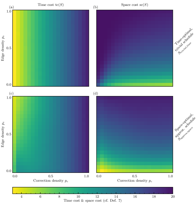
Figure 2: Time and space costs (cf. Def. 7) for the trivial time-optimal schedule and the approximated space-optimal schedule, for $\left\lvert V\right\rvert=20$ vertices. (a) shows the time cost $\mathrm{tc}$ for the time-optimal schedule $S_{\text{trivial,time}}$ directly obtained from the time order induced by the Pauli frames. Up to numerical errors, the time cost is independent of the edge density $p_{e}$ and increases with the correction density $p_{c}$. (b) shows the space cost $\mathrm{sc}$ for the same schedule $S_{\text{trivial,time}}$. (c) and (d) show the according costs for the approximated space-optimal schedules $S_{\text{approx,space}}$, respectively. For details about the probabilistic approximated search , look at App. A.

In Figs. 2 and 3 we show some numerical results of the space and time costs for random graphs and time orders. The results are not directly based on quantum circuits but rather on random graphs and random time orders. The graphs are randomly generated by uniformly creating edges with a certain density $p_{e}$. Instead of directly drawing a random time order, we draw random Pauli frames and then calculate the time order from them using the Pauli tracking library. We do this, to create a closer connection to the underlying MBQC scheduling problem: First, we randomly pick one vertex, which represents a vertex/qubit in a teleportation protocol that is going to be “measured” (cf. Fig. 1). Then, we randomly induce Pauli corrections on the other vertices (which have not been “measured” yet), dependent on the picked vertex, with a certain probability $p_{c}$. These corrections form a random Pauli frame that represents the correction induced by the picked vertex, which would have been tracked through a hypothetical circuit. This way, one might argue that the correction density $p_{c}$ resembles the spreading of the induced Pauli corrections because of entanglement.

Alternatively, to have a closer relation to quantum algorithms, we could have directly drawn random circuits, or maybe specific circuits, and then use different MBQC protocols to transform them into graphs and time orders. However, this compilation is not trivial to implement and not part of this project.

Keeping this in mind, the shown results should be viewed as qualitative indications whether it might be worth to invest in this optimisation technique. They are definitely not benchmarks, since sampling enough data in a stable environment would require extremely long calculations due to the hardness of the problem. Furthermore, in an application, it will also heavily depend on the specific quantum algorithm, the MBQC protocol, and the underlying hardware which puts additional constraints on the scheduling.

Figure 2 shows the time cost for the trivial time-optimal schedule and the space cost for an approximated space-optimal schedule, for a fixed number of vertices, $\left\lvert V\right\rvert=20$, but different edge densities $p_{e}$ and correction densities $p_{c}$. The time cost for the time-optimal path (Fig. 2 (a)) is completely independent of the edge density $p_{e}$; this is clear, since it is directly calculated from the time order, without any reference to the graph. The lower the correction density $p_{c}$ is, the lower is the time cost. This is because the time order has less order relations, implying less layers in the directed time order graph, on average. Regarding the space cost for the approximated space-optimal schedule, (Fig. 2 (d)) we see that it increases rather fast with the edge density $p_{e}$. The reason for that is that more vertices have to be initialised when we want to measure a vertex, according to Def. 6 (a), since the vertex has more neighbours. With increasing correction density $p_{c}$, there are less choices to measure first a vertex with less neighbours (Def. 6 (b)), and therefore the cost increases. The other two plots, Fig. 2 (b) and (c), show mainly artefacts of how the algorithm is implemented: For low correction densities the space cost of the trivial time-optimal schedule is high because this schedule greedily measures as many vertices as possible. The time cost for the approximated space-optimal schedule decreases with the correction density, because the algorithm always first tries the more time-optimal schedules.

While these plots are not based on real quantum circuits, they confirm the expected behaviour of the costs and maybe provide some qualitative intuition for when it is worth to search for a more space-optimal schedule, if this is wanted. For example, if the edge density is relatively high, e.g., $p_{e}>0.8$, and the correction density is not too low, e.g., $p_{c}>0.6$, it might not be worth searching for a space-optimal schedule because the space cost probably cannot be reduced significantly. On the other hand, if the edge density is low, the space cost can probably be significantly reduced.

In Fig. 3 we can see analogue costs, but now for a varying number of vertices $\left\lvert V\right\rvert$. The edge and correction densities scale via $p_{e}\left\lparen\left\lvert V\right\rvert\right\rparen=p_{c}\left\lparen\left\lvert V\right\rvert\right\rparen=0.5/\sqrt{\left\lvert V\right\rvert-1}$. This is equivalent to the vertex degree scaling with $\sqrt{\left\lvert V\right\rvert-1}$. Importantly, in the asymptotic limit $\left\lvert V\right\rvert\to\infty$, it is $p_{e}\left\lparen\left\lvert V\right\rvert\right\rparen>\ln\left\lparen\left\lvert V\right\rvert\right\rparen/\left\lvert V\right\rvert$, which ensures that the graph is connected almost surely (cf., e.g., [30], more specifically see ). Notably, we see that the space costs for the approximated space-optimal schedule are close to the exact space-optimal schedule, at least up to the number of vertices for which we performed the exact optimisation (with much faster run-times, cf. Fig. 4). For larger graphs, however, this deviation would of course increase. Furthermore, the space cost of the time-optimal schedule obtained from the exact optimisation is lower than the space cost of the trivial time-optimal schedule. This is because the trivial time-optimal schedule does not try to measure first vertices with less neighbours.

For additional information about the numerical data, e.g., which probabilistic acceptance function is chosen or for recorded run-times, see App. A.

In general, the results show that appropriate scheduling of qubit initialisation and measurement can potentially greatly reduce the space and time cost, depending on the system parameters (especially compared to just naively initialising the whole graph). Finding optimal schedules, however, is a hard problem, and will require optimised algorithms for larger scales. The trivial time-optimal schedule, however, can be obtained in polynomial time from appropriately tracked Pauli frames. In an application, one can imagine starting with the trivial order and then trying to optimise it with respect to space, until a certain space cost is reached or stop the optimisation after a certain timeout.

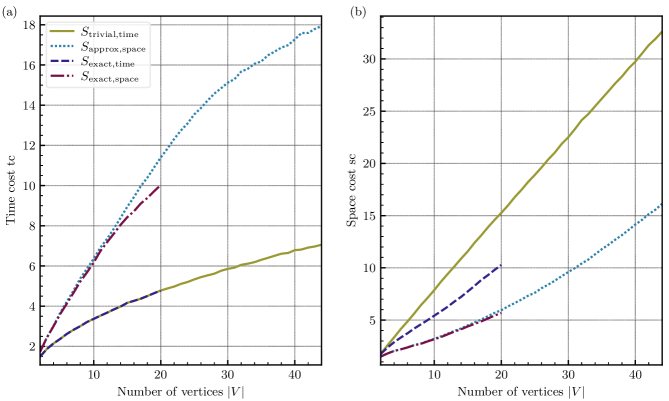
Figure 3: The time and space costs depending on the number of vertices $\left\lvert V\right\rvert$. The edge and correction densities scale with $\left\lvert V\right\rvert$: $p_{e}=p_{c}=0.5/\sqrt{\left\lvert V\right\rvert-1}$. (a) shows the time cost $\mathrm{tc}$ and (b) the space cost $\mathrm{sc}$ for different schedules. $S_{\text{trivial,time}}$ and $S_{\text{approx,space}}$ are the trivial time-optimal schedule and approximated space-optimal schedule as in Fig. 2. $S_{\text{exact,time}}$ and $S_{\text{exact,space}}$ are the according data of a full search for exact optimality, that is, $S_{\text{exact,time}}$ is a time-optimal schedule with the lowest possible space cost and $S_{\text{exact,space}}$ is a space-optimal schedule with the lowest possible time cost. These exact data points are only calculated for $\left\lvert V\right\rvert\leq 20$ since the run-time becomes very long. It is $\mathrm{tc}\left\lparen S_{\text{exact,time}}\right\rparen=\mathrm{tc}\left\lparen S_{\text{trivial,time}}\right\rparen$ and the costs for $S_{\text{approx,space}}$ are close to the costs of $S_{\text{exact,space}}$, however, $\mathrm{sc}\left\lparen S_{\text{exact,time}}\right\rparen$ is fairly lower than $\mathrm{sc}\left\lparen S_{\text{trivial,time}}\right\rparen$.

4 Conclusion

We presented a software library that provides the functionality to track Pauli gates through a (Clifford) quantum circuit. The library is designed to be low level and generic, allowing easy integration into other projects. The library is based on the isomorphism between the Clifford group and the symplectic group. Tracking Pauli gates allows to reduce the number of Pauli gates to the number of qubits or less. Furthermore, when tracking Pauli corrections in MBQC, the information can be used to calculate the strict partial (time) order of the measurements. This allows us to perform scheduling optimisations, which we tackled in the second part of the paper. We presented a framework that covers the scheduling problem on an abstract level reduced to the underlying graph and the time order. The numerical results we showed give indications on how much can be gained with this optimisation technique, however, one has to keep in mind that the optimisation is a computational hard problem, which is how we calculated the data for the approximated space-optimal schedules.

5 Software Availability

The source code of the Pauli tracking library can be found in the taeruh/pauli_tracker repository on GitHub [16]. The Rust library is published on crates.io and the Python wrapper on pypi.org where you can also find links to the documentation. For the source code of the MBQC scheduling project, see taeruh/mbqc_scheduling [28].

Appendix A More on the numerical results

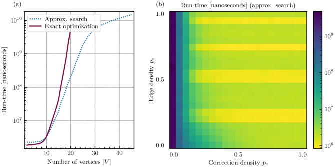
Figure 4: Recorded run-times of the calculations. This is not a benchmark. In both plots the run-time is the average time it took to perform the optimisation, given a graph and a time order. (a) shows how the approximate algorithm performs compared to the exact algorithm, w.r.t. the number of vertices $\left\lvert V\right\rvert$. Considering the logarithmic scale, it is magnitudes faster. Starting at approximately $30$ vertices, the timeout that scales quadratically with the number of vertices is reached, and the search returns early. (b) shows how the run-time depends on the edge density $p_{e}$ and the correction density $p_{c}$. It drastically increases for low correction densities. Vertically, for different edge densities, there are discontinuities. This is because for each selected edge density, the according data points, w.r.t. the correction density, were calculated on a different cluster node which were under different load (running the simulations on smaller grids locally on a single laptop does not show these discontinuities).

The code for the data generation and the numerical data can be found at the commits 6aaa4d8 and 040e289 in taeruh/mbqc_scheduling/results [28], respectively. The data capture all the information that is needed to reproduce the data. However, an exact reproduction for the approximated results is impossible. This is because the algorithm is multi-threaded and the tasks that are sent to the threads communicate intermediate results between each other, which change how the tasks continue their execution. While this is in theory deterministic, in practice it depends on how the operating system schedules the threads and what the CPU is doing.

The probabilistic acceptance function that we used for the approximated space-optimal schedules is given by

$$p_{\mathrm{accept}}\left\lparen\Delta\mathchar 44\relax V\mathchar 44\relax M\right\rparen=\Theta\left\lparen\left\lvert\Delta\right\rvert\right\rparen\left\lvert V\right\rvert^{2}\mathrm{e}^{-\frac{\left\lvert V\right\rvert\left\lvert V{\setminus}M\right\rvert}{\left\lvert\Delta\right\rvert^{3}\left\lparen\left\lvert M\right\rvert\right\rparen}}$$ (4)

where $V$ are the vertices in the graph, $M$ are the vertices that have been measured so far (including the ones in the currently picked measurement set), $\Delta$ the difference between the best memory and the required memory so far, and $\Theta$ is the Heaviside step function (being $1$ for positive elements). The step function ensures that we only focus on space-optimal schedules. For finding schedules somewhere between space optimal and time optimal, i.e., a full space-time optimisation, one can choose a smoother function. The exponential decay ensures that the run-time is sufficiently small for our experiments, focusing on schedules with a rather large space improvement. In a real application, e.g., a real quantum compiler toolchain, one may choose a more optimised function, fitting to the required needs, and optimise its parameters.

The probabilistic searches have a timeout which increases quadratically with the number of qubits, i.e., we stop the search after $\mathcal{O}\left\lparen\left\lvert V\right\rvert^{2}\right\rparen$ time and return the best results that have been found so far. The effect of that can be seen in Fig. 4 (b), where the run-time drops down onto a quadratic curve for larger number of qubits, however, note that the behaviour of the according curves in Fig. 3 indicate that the implied penalty on the costs is not too high.

The standard deviations, which we do not show for simplicity, on the plotted results are relatively high. This is an artefact of combinatorics: For small number of vertices, the standard deviation is just relatively high, and for larger number of vertices it becomes a sampling issue. Because of that, we emphasise again that the results are rather qualitative indications than quantitative benchmarks.

In Fig. 4 we see the average run-time for the calculations. This is not a benchmark, but only shows the recorded run-times for our calculations. The calculations were performed on a cluster where the vertices were under different loads; therefore, these plots are only qualitative indications. We see that the approximate optimisation runs much faster than the exact search for larger graphs. In general, the run-time heavily depends on the chosen acceptance function Eq. 4. For small correction densities, the run-time drastically increases, because the number of possible measurement steps, per step, scales according to the ordered Bell numbers.

References

- [1] Robert Raussendorf and Hans J. Briegel. “A one-way quantum computer”. Phys. Rev. Lett. 86, 5188–5191 (2001).
- [2] Vincent Danos, Elham Kashefi, and Prakash Panangaden. “The measurement calculus”. J. ACM 54, 8–es (2007). arXiv:0704.1263.
- [3] E. Knill. “Quantum computing with realistically noisy devices”. Nature 434, 39–44 (2005). arXiv:quant-ph/0410199.
- [4] Alexandru Paler, Simon Devitt, Kae Nemoto, and Ilia Polian. “Software-based Pauli tracking in fault-tolerant quantum circuits”. Design, Automation & Test in Europe Conference & ExhibitionPages 1–4 (2014). arXiv:1401.5872.
- [5] L. Riesebos, X. Fu, S. Varsamopoulos, C. G. Almudever, and K. Bertels. “Pauli frames for quantum computer architectures”. Proceedings of the 54th Annual Design Automation Conference 76, 1–6 (2017).
- [6] Jin-Ho On, Chei-Yol Kim, Soo-Cheol Oh, Sang-Min Lee, and Gyu-Il Cha. “A multilayered Pauli tracking architecture for lattice surgery-based logical qubits”. ETRI Journal 45, 462–478 (2023).
- [7] S. B. Bravyi and A. Yu. Kitaev. “Quantum codes on a lattice with boundary” (1998).
- [8] Austin G. Fowler, Matteo Mariantoni, John M. Martinis, and Andrew N. Cleland. “Surface codes: Towards practical large-scale quantum computation”. Physical Review A 86, 032324 (2012). arXiv:1208.0928.
- [9] Daniel Gottesman and Isaac L. Chuang. “Demonstrating the viability of universal quantum computation using teleportation and single-qubit operations”. Nature 402, 390–393 (1999). arXiv:quant-ph/9908010.
- [10] Xinlan Zhou, Debbie W. Leung, and Isaac L. Chuang. “Methodology for quantum logic gate construction”. Phys. Rev. A 62, 052316 (2000). arXiv:quant-ph/0002039.
- [11] Beverley Bolt, T. G. Room, and G. E. Wall. “On the Clifford collineation, transform and similarity groups. i.”. Journal of the Australian Mathematical Society 2, 60–79 (1961).
- [12] Beverley Bolt, T. G. Room, and G. E. Wall. “On the Clifford collineation, transform and similarity groups. ii.”. Journal of the Australian Mathematical Society 2, 80–96 (1961).
- [13] Beverley Bolt. “On the Clifford collineation, transform and similarity groups. (iii) generators and involutions”. Journal of the Australian Mathematical Society 2, 334–344 (1962).
- [14] Daniel Gottesman. “The Heisenberg representation of quantum computers” (1998).
- [15] Craig Gidney. “Stim: a fast stabilizer circuit simulator”. Quantum 5, 497 (2021). arXiv:2103.02202.
- [16] Pauli-Tracker contributors. “Pauli tracker: A library to track Pauli gates through Clifford circuits” (2024). avalaible at https://github.com/taeruh/pauli_tracker.
- [17] Madhav Krishnan Vijayan, Alexandru Paler, Jason Gavriel, Casey R Myers, Peter P Rohde, and Simon J Devitt. “Compilation of algorithm-specific graph states for quantum circuits”. Quantum Science and Technology 9, 025005 (2024). arXiv:2209.07345.
- [18] T. Le et al. “BenchQ project” (2024). In preparation.
- [19] Samuel J. Elman, Jason Gavriel, and Ryan L. Mann. “Optimal scheduling of graph states via path decompositions” (2024). arXiv:2403.04126.
- [20] Earl T. Campbell and Mark Howard. “Unified framework for magic state distillation and multiqubit gate synthesis with reduced resource cost”. Phys. Rev. A 95, 022316 (2017).
- [21] Peter Selinger. “Generators and relations for n-qubit Clifford operators”. Logical Methods in Computer Science 11, 2 (2015). arXiv:1310.6813.
- [22] Pauli-Tracker contributors. “Supported Clifford gates in the library at the time of writing” (2024). taeruh/pauli_tracker/docs/conjugation_rules.
- [23] D. Gross. “Hudson’s theorem for finite-dimensional quantum systems”. Journal of Mathematical Physics47 (2006). arXiv:quant-ph/0602001.
- [24] Maurice R Kibler. “Variations on a theme of Heisenberg, Pauli and Weyl”. Journal of Physics A: Mathematical and Theoretical 41, 375302 (2008). arXiv:0807.2837.
- [25] J Tolar. “On Clifford groups in quantum computing”. Journal of Physics: Conference Series 1071, 012022 (2018). arXiv:1810.10259.
- [26] Circ contributors. “Circ: An open source framework for programming quantum computers” (2023).
- [27] Qiskit contributors. “Qiskit: An open-source framework for quantum computing” (2023).
- [28] MBQC-Scheduling contributors. “MBQC scheduling: Scheduling in measurement-based quantum computing” (2024). available at https://github.com/taeruh/mbqc_scheduling.
- [29] Ralph W. Bailey. “The number of weak orderings of a finite set”. Social Choice and Welfare 15, 559–562 (1998).
- [30] Joel Spencer. “Ten lectures on the probabilistic method”. Society for Industrial and Applied Mathematics. (1994). 2nd edition edition.
- MBQC
- measurement-based quantum computation
- NISQ
- noisy intermediate-scale quantum (computing)
- QEC
- quantum error correction
- SIMD
- single instruction, multiple data (CPU instruction)