Charged lepton-flavor violating constraints to non-unitarity in the Linear Seesaw scheme

Abstract

We analyze the non-unitary effects in the linear seesaw mechanism using the current constraints and future sensitivity of the charged Lepton Flavor Violation (cLFV) processes. We perform a random scan confronting the non-unitary parameters with the limits to the cLFV processes. We show our results for the normal and inverted ordering of the oscillation data. We also discuss the equivalence of different parametrizations of the non-unitary mixing matrix and show our results in terms of the different parameterizations. We found that the stronger restrictions in the non-unitary parameter space come from rare muon decay searches.

I Introduction

Just after the proposal of the Standard Model (SM), the efforts for a new physics model that explains the observed nature of elementary particles as minimal as possible have been constantly growing. The confirmation of neutrino oscillations, which implies that neutrinos have a mass different from zero, boosted the search for new physics in the neutrino sector. Of particular interest are the seesaw mechanisms [1, 2, 3, 4, 5, 6] that aim precisely to explain the smallness of the neutrino masses involved in oscillations, adding right-handed heavy neutral states. These heavy right-handed neutrinos are singlets under the SM gauge symmetry and generate the suppression relation between the light and heavy neutrino mass. Moreover, low-scale seesaw mechanisms like the inverse [7] and linear [8, 9] seesaw have the extra characteristic that they could be realized at a relatively lower mass scales, making them more attractive, as they can be tested in the near future accelerators [10]. Besides, there are also searches for indirect evidence of the Heavy Neutral Leptons (HNL) due to the non-unitary of the $3\times 3$ lepton mixing matrix [11, 12].

Besides the different searches for signatures of neutral heavy leptons in accelerators through direct production, it is also expected that HNL may induce lepton flavor violation. This work will focus on charged lepton flavor violation (cLFV) observables, studying current constraints on the branching ratios and future expected sensitivities. For cLFV observables, the predicted branching ratio will depend on the neutral mass eigenstates and on the new mixing matrix parameters. Given a neutrino mass pattern, we can compute the branching ratio in terms of the light mixing sector, allowing for constraints on the non-unitary parameters. We will study this phenomenology in the context of the linear seesaw mechanism. Previous works in a similar direction exist in the literature [10, 13]. For example, the case of the inverse seesaw was already studied [14], and thorough studies with previous data have also been carried out [15].

This work is organized as follows: section II describes the general seesaw mechanism, the low-scale (linear) mechanism and the nonunitary effects in both schemes. The section III describes the flavor violation processes and contains all the numerical aspects of our analysis and all the parametrizations that we follow. Section IV presents the sensitivity of the nonunitary parameters and the phase space of the linear seesaw in these flavor violation processes and shows our conclusions.

II seesaw mechanism

A simple and natural way to explain the neutrino tiny masses is the well-known seesaw type-I mechanism [2, 1, 4, 3]. In this model, the mass matrix has the following form:

$$M_{n\times n}=\begin{pmatrix}0&M_{D}\\ M^{T}_{D}&M_{R}\end{pmatrix}.$$ (1)

There is no limit for the number of singlets that can be added in the theory. The physical neutrino masses are obtained by diagonalizing Eq. (1)

$$U^{T}M_{n\times n}U=M_{diag}.$$ (2)

There are different ways to compute the matrix U. Let’s consider that, at leading order, it takes the form [16, 17]

$$U=\text{\~{U}}\cdot V,$$ (3)

where Ũ=$e^{iH}$, with

$$H=\begin{pmatrix}0&S\\ S^{\dagger}&0\end{pmatrix},\quad V=\begin{pmatrix}V_{1_{3\times 3}}&0\\ 0&V_{2_{m\times m}}\end{pmatrix}.$$ (4)

We assume that the main contribution for diagonalizing the neutrinos mass matrix comes from $V_{1_{3\times 3}}$ and $V_{2_{m\times m}}$ while $S$ should give play a sub-leading role in this diagonalization process. After expanding in series we can get

$$\text{\~{U}}\simeq\begin{pmatrix}(\mathbb{I}-\frac{1}{2}SS^{\dagger})_{3\times 3}&iS_{3\times m}\\ iS^{\dagger}_{m\times 3}&(\mathbb{I}-\frac{1}{2}S^{\dagger}S)_{m\times m}\end{pmatrix},$$ (5)

with $m=n-3$. Considering that we must fulfill Eq. (2) we can express Ũ as [15, 14]

$$\text{\~{U}}=\begin{pmatrix}\mathbb{I}_{3\times 3}-\frac{1}{2}(M_{D}^{*}(M^{*}_{R})^{-1}M^{-1}_{R}M^{T}_{D})_{3\times 3}&(M^{*}_{D}(M_{R}^{*})^{-1})_{3\times m}\\ (M_{R}^{-1}M^{T}_{D})_{m\times 3}&\mathbb{I}_{3\times 3}-\frac{1}{2}(M^{-1}_{R}M^{T}_{D}M_{D}^{*}(M^{*}_{R})^{-1})_{m\times m}\end{pmatrix}.$$ (6)

Using Eqs. (2) and (6), we get:

$$m_{diag}= (V_{1}^{T}m_{\nu}V_{1})_{3\times 3}$$ (7)

$$M^{diag}_{N}= (V_{2}^{T}M_{N}V_{2})_{m\times m}.$$ (8)

We can observe that $V_{1}$ and $V_{2}$ are unitary matrices and diagonalize the light and heavy sectors respectively. At leading order, $m_{\nu}$ and $m_{N}$ are given by:

$$m_{\nu}\simeq -(M_{D}M^{-1}_{R}M^{T}_{D})_{3\times 3}$$ (9)

$$M_{N}\simeq M_{R}$$ (10)

Nonunitarity effects

The new extra heavy neutrino massive states induce effects in the light sector. We can observe that the light sector is no longer unitarity, unlike the standard oscillation paradigm. Nonunitary signals have been searched for in the literature since it will be a clear probe of physics beyond the Standard Model [18, 19, 20, 21, 22, 23, 24, 25, 26]. To study the nonunitary effects, we can use the rectangular matrix $K_{ij}$ that characterizes the charge current interaction for leptons. It can be seen in the following lagrangian:

$$\mathcal{L}=-\frac{g}{\sqrt{2}}W^{-}_{\mu}\sum^{3}_{i=1}\sum^{n}_{j=1}K_{ij}\bar{l}_{i}\gamma^{\mu}P_{L}\nu_{j}+h.c.,$$ (11)

where

$$K_{ij}=\sum^{3}_{c=1}\Omega^{*}_{ci}U_{cj}.$$ (12)

and the subscript $j$ runs along all the neutrino states, including the heavy ones. The $\Omega_{ci}$ is the charged lepton mixing matrix; in this work, we assume it is diagonal ($\Omega_{ci}=\delta_{ci}$), so the matrix K depends totally on the neutrino mixing matrix. It is useful to describe the matrix K as block matrices:

$$K=(N,S),$$ (13)

where N describes the mixing with the light sector, and S with the heavy one. Using Eqs. (3) and (6), we get

$$N= \mathbb{I}_{3\times 3}-\frac{1}{2}(M_{D}^{*}(M^{*}_{R})^{-1}M^{-1}_{R}M^{T}_{D})_{3\times 3}V_{1},$$ (14)

$$S= (M^{*}_{D}(M_{R}^{*})^{-1})_{3\times m}V_{2}.$$ (15)

The nonunitary effects are related to the light sector, in other words with the N block matrix. We can parametrize the nonunitary deviation as:

$$N=(\mathbb{I}-\eta)V_{1},$$ (16)

where $\eta$ describes the nonunitary effects in terms of the $M_{D}$ and $M_{R}$,

$$\eta=\frac{1}{2}(M_{D}^{*}(M^{*}_{R})^{-1}M^{-1}_{R}M^{T}_{D})_{3\times 3}.$$ (17)

Originally, this type-I seesaw model was motivated by Grand Unification Theories. Therefore, in that case, the NHL masses were expected at high energy scales, of the order of the GUT scale. Currently, well-motivated low-energy realizations of the seesaw mechanism are being considered since the expected mass scales might be close to the energy range of near future accelerator experiments. This is the case of the Linear seesaw mechanism that we consider in this work.

Linear seesaw mechanism

In several low-scale realizations of the type-I seesaw mechanism, such as the linear seesaw, instead of adding only three singlets under $SU(2)$, the number of additional NHL is extended to be six. The mass matrix in the linear seesaw has the form [9]:

$$M_{\nu}=\begin{pmatrix}0&M_{D}&M_{L}\\ M^{T}_{D}&0&M\\ M^{T}_{L}&M^{T}&0\end{pmatrix}.$$ (18)

All the components in this matrix are $3\times 3$ block matrices. Our purpose is to analyze the lepton flavor violation phenomenology of this well motivated scheme. The most important requirement in our analysis is to respect the hierarchy $M_{L}<<M_{D}<<M$.

To diagonalize Eq. (18), it is usual to define the following matrices:

$$M_{DL}= (M_{D},M_{L})_{3\times 6}\quad M^{T}_{DL}=\begin{pmatrix}M^{T}_{D}\\ M^{T}_{L}\end{pmatrix}_{6\times 3},$$ (19)

$$M_{R_{6\times 6}}= \begin{pmatrix}0&M\\ M^{T}&0\end{pmatrix}\quad(M_{R_{6\times 6}})^{-1}=\begin{pmatrix}0&(M^{T})^{-1}\\ M^{-1}&0\end{pmatrix}$$ (20)

and diagonalize by blocks to get the light and heavy masses

$$m_{\nu}=M_{D}(M_{L}M^{-1})^{T}+(M_{L}M^{-1})M^{T}_{D},\quad M_{N}=M_{R_{6\times 6}}.$$ (21)

We have that the rectangular matrix, equivalent to Eq. (13), has the form

$$K^{LS}=(N^{LS}_{3\times 3},S^{LS}_{3\times 6}),$$ (22)

where (LS) is for Linear Seesaw. In the limit $M_{L}\longrightarrow 0$, the submatrices take the form

$$N^{LS}=(\mathbb{I}_{3\times 3}-\eta^{LS}_{3\times 3})\cdot V_{1_{3\times 3}},\quad S^{LS}=(0_{3\times 3},(M^{*}_{D}(M^{*T})^{-1})_{3\times 3})\cdot V_{2_{6\times 6}}$$ (23)

and the nonunitary effects are characterized by:

$$\eta^{LS}=\frac{1}{2}(M_{D}^{*}(M^{*})^{-1}M^{-1}M^{T}_{D})_{3\times 3}.$$ (24)

Matching the non-unitary effects in the different parametrizations

The mixing matrix that we see above comes from the type-I seesaw mechanism. However, it is not the only realization of the mixing matrix, an example is the symmetric parametrization. Therefore, we have another way to describe the non-unitary effects in the light sector and we want to match the $\eta$ parameters with the non-unitary parameters on this parametrization. The relevance of the symmetric parametrization lies in the constraints on the non-unitary parameters obtained from oscillation experiments [27, 28, 29]. In this parametrization, each mixing angle has a Majorana phase. For instance,

$$\omega_{13}=\begin{pmatrix}\cos\theta_{13}&0&\sin\theta_{13}e^{-i\phi_{13}}\\ 0&1&0\\ -\sin\theta_{13}e^{i\phi_{13}}&0&\cos\theta_{13}\end{pmatrix}.$$ (25)

The standard $3\times 3$ leptonic mixing matrix is written in this case as $\omega_{23}\omega_{13}\omega_{12}$. We can extend the matrix as many new neutrinos as we want, and the light sector is described as follows [12]:

$$N=N^{\mathrm{NP}}U^{SM}=\begin{pmatrix}\alpha_{11}&0&0\\ \alpha_{21}&\alpha_{22}&0\\ \alpha_{31}&\alpha_{32}&\alpha_{33}\end{pmatrix}U^{SM},$$ (26)

where $N^{NP}$ parametrize the deviation from the unitary in the light sector. This parametrization is important in constraining non-unitary effects in oscillation experiments.

The non-unitary effect in the symmetrical parametrization is a complete description of the light sector and it can be compared with the parametrization in terms of the $\eta$ matrix. We can also obtain an expression in terms of the extra mixing angles when we consider that they are small. For this purpose, we approximate the mixing matrix to quadratic terms in the mixing angle that are related to the active neutrinos and the NHLs. For example, to describe explicitely the mixing matrix in the $3+3$ case we have

$$U^{6x6} = \omega_{56}\omega_{46}\omega_{36}\omega_{26}\omega_{16}\omega_{45}\omega_{35}\omega_{25}\omega_{15}\omega_{34}\omega_{24}\omega_{14}\omega_{23}\omega_{13}\omega_{12},$$ (27)

$$= U^{NP}U^{3x3}$$

where the product of the last three matrices $U^{3x3}=\omega_{23}\omega_{13}\omega_{12}$ describes the mixing of the light neutrino sector with the three standard active neutrinos. On the other hand, the first products describe the mixing of the light and heavy sector with the additional NHLs

$$U^{NP}=\omega_{56}\omega_{46}\omega_{36}\omega_{26}\omega_{16}\omega_{45}\omega_{35}\omega_{25}\omega_{15}\omega_{34}\omega_{24}\omega_{14}.$$ (28)

This particular ordering for the multiplication of the matrices gives rise to the triangular parametrization described by the submatrix $N^{NP}$. We can go a step forward and rearrange this matrix to separate it into two different parts without loosing the triangular property for $N^{NP}$. We first notice that the matrix $\omega_{45}$ conmutes with the product $\omega_{36}\omega_{26}\omega_{16}$ since the mixings acts on different rows and columns. Due to this property, we can rearrange the matrix in Eq. (28), without changing parametrization, as

$$U^{NP}=\omega_{56}\omega_{46}\omega_{45}\omega_{36}\omega_{26}\omega_{16}\omega_{35}\omega_{25}\omega_{15}\omega_{34}\omega_{24}\omega_{14}$$ (29)

Notice that the matrices that mix the heavy sector are now grouped:

$$U^{H}=\omega_{56}\omega_{46}\omega_{45}.$$ (30)

On the other hand, those that mix the additional NHLs with the light neutrino states appears to the right of $U^{NP}$:

$$U^{LH}=\omega_{36}\omega_{26}\omega_{16}\omega_{35}\omega_{25}\omega_{15}\omega_{34}\omega_{24}\omega_{14}.$$ (31)

In this way, we can separate the complete $n\times n$ mixing matrix into the product of three different matrices that contain the information of the purely heavy sector, $U^{H}$, the purely light sector, $U^{3\times 3}$, and the mixing of both sectors, $U^{LH}$, respectively. Notice that this separation can be applied irrespectively of the number of extra NHLs. We restrict here to the $6\times 6$ case but the same method applies in general.

The full mixing matrix in this $6\times 6$ example can then be written as

$$U^{6\times 6}=U^{H}U^{LH}U^{3\times 3}=\begin{pmatrix}I_{3\times 3}&0_{3\times 3}\\ 0_{3\times 3}&H_{3\times 3}\end{pmatrix}U^{LH}\begin{pmatrix}U^{SM}&0_{3\times 3}\\ 0_{3\times 3}&I_{3\times 3}\end{pmatrix}.$$ (32)

Where $U^{SM}$ and $H_{3\times 3}$ are unitary matrices. As we can see the deviation of the unitary in the light sector comes from the $U^{LH}$ matrix. After this rearrangement, it is evident that the submatrix $N^{NP}$ will not have any contribution from the "heavy-heavy” mixing angles and will depend only on angles (and phases) of the form $\theta_{1n},\theta_{2n},\theta_{3n}$, with $n>3$.

Using the approximation where we consider the new mixing angles up to order 2, the light sector of $U^{LH}$ is:

$$\begin{pmatrix}\alpha_{11}&0&0\\ \alpha_{21}&\alpha_{22}&0\\ \alpha_{31}&\alpha_{32}&\alpha_{33}\end{pmatrix}\approx I_{3\times 3}-\begin{pmatrix}\frac{1}{2}(\theta^{2}_{14}+\theta^{2}_{15}+\theta^{2}_{16})&0&0\\ \hat{\theta}_{16}\hat{\theta}^{*}_{26}+\hat{\theta}_{15}\hat{\theta}^{*}_{25}+\hat{\theta}_{14}\hat{\theta}^{*}_{24}&\frac{1}{2}(\theta^{2}_{24}+\theta^{2}_{25}+\theta^{2}_{26})&0\\ \hat{\theta}_{16}\hat{\theta}^{*}_{36}+\hat{\theta}_{15}\hat{\theta}^{*}_{35}+\hat{\theta}_{14}\hat{\theta}^{*}_{34}&\hat{\theta}_{26}\hat{\theta}^{*}_{36}+\hat{\theta}_{25}\hat{\theta}^{*}_{35}+\hat{\theta}_{24}\hat{\theta}^{*}_{34}&\theta^{2}_{14}+\theta^{2}_{15}+\theta^{2}_{16}\end{pmatrix}.$$ (33)

Where $\hat{\theta}_{ij}=\theta_{ij}e^{i\phi_{ij}}$. We can generalize this approximated matrix for the case of an arbitrary number of new neutral heavy leptons:

$$\begin{pmatrix}\sum_{j=4}^{n}\frac{1}{2}(\theta^{2}_{1j})&0&0\\ \sum_{j=4}^{n}\hat{\theta}_{1j}\hat{\theta}^{*}_{2j}&\sum_{j=4}^{n}\frac{1}{2}(\theta^{2}_{2j})&0\\ \sum_{j=4}^{n}\hat{\theta}_{1j}\hat{\theta}^{*}_{3j}&\sum_{j=4}^{n}\hat{\theta}_{2j}\hat{\theta}^{*}_{3j}&\sum_{j=4}^{n}\frac{1}{2}(\theta^{2}_{3j})\end{pmatrix}=\begin{pmatrix}\alpha^{\prime}_{11}&0&0\\ \alpha^{\prime}_{21}&\alpha^{\prime}_{22}&0\\ \alpha^{\prime}_{31}&\alpha^{\prime}_{32}&\alpha^{\prime}_{33}\end{pmatrix}=\alpha^{\prime}_{3\times 3},$$ (34)

where n is the total number of neutrinos.

To find the equivalence between the two different parametrizations, we compute the expression for $NN^{\dagger}$ in both cases:

$$NN^{\dagger} =(\mathbb{I}-\eta)(\mathbb{I}-\eta)^{\dagger}=\mathbb{I}-2\eta+\mathcal{O}(2)$$ (35)

$$NN^{\dagger} =(\mathbb{I}-\alpha^{\prime})(\mathbb{I}-\alpha^{\prime})^{\dagger}=\mathbb{I}-(\alpha^{\prime}+\alpha^{\prime^{\dagger}})+\mathcal{O}(2)$$ (36)

$$\eta =\frac{1}{2}(\alpha^{\prime}+\alpha^{\prime^{\dagger}})=\frac{1}{2}\begin{pmatrix}2\alpha^{\prime}_{11}&\alpha^{\prime^{*}}_{21}&\alpha^{\prime^{*}}_{31}\\ \alpha^{\prime}_{21}&2\alpha^{\prime}_{22}&\alpha^{\prime^{*}}_{32}\\ \alpha^{\prime}_{31}&\alpha^{\prime}_{32}&2\alpha^{\prime}_{33}\end{pmatrix},$$ (37)

in accordance with [30]. Now we have a relation between both parametrization and constraints for $\eta$ elements are constraints to $\alpha$ parameters.

III cLFV and numerical analysis

Heavy neutral leptons within the type I seesaw framework contribute to lepton flavor violation processes due to their mixing with the active SU(2) doublet neutrinos. We will focus on processes of the type $\ell_{i}\longrightarrow\ell_{j}\gamma$, where $\ell_{i}$ could be a $\tau$ or a $\mu$, and $\ell_{j}$ stands for e or $\mu$. In general, these branching ratios are given by [31]

$$Br(\ell_{i}\longrightarrow\ell_{j}\gamma)=\frac{\alpha^{3}_{W}s^{2}_{W}}{256\pi^{2}}\frac{m^{5}_{\ell_{1}}}{M^{4}_{W}}\frac{1}{\Gamma_{\ell_{i}}}|G^{W}_{ij}|^{2},$$ (38)

where

$$G^{W}_{ij}= \sum_{k=1}^{9}K^{*}_{ik}K_{jk}G^{W}_{\gamma}\left(\frac{m^{2}_{i}}{M_{W}^{2}}\right),$$

$$G^{2}_{\gamma}(x)= \frac{1}{12(1-x)^{4}}(10-43x+78x^{2}-49x^{3}+18x^{3}lnx+4x^{4}),$$ (39)

$M_{W}$ is the boson W mass, $m_{i}$ is the physical neutrino mass, and $\alpha_{W}\equiv\alpha/s^{2}_{W}$ with $\alpha=e^{2}/4\pi$ the fine structure constant and $s_{W}$ the Weinberg angle. We will analyze the nonunitary effects using the current constraints and the future sensitivity of these processes, summarized in Table 1, as reported in [14].

Process	Present limit	Future Sensitivity
$\mu\longrightarrow e\gamma$	$4.2\times 10^{-13}$ [32]	$6\times 10^{-14}$ [33]
$\tau\longrightarrow e\gamma$	$3.3\times 10^{-8}$ [34]	$3\times 10^{-9}$[35]
$\tau\longrightarrow\mu\gamma$	$4.2\times 10^{-8}$ [34]	$10^{-9}$ [35]

Table 1: The current limits and expected future sensitivity for the flavor violations processes,

To reduce the number of degrees of freedom of our analysis, we will work in a scheme where $M_{L}$ and $M$ are diagonal and real. We will assume that the flavor violation is only due to the Dirac Yukawa coupling [36]. To write the Dirac mass matrix, we use the Casas-Ibarra parametrization applied to the linear seesaw [15, 37].

$$M_{D}=V^{*}_{1}\sqrt{m^{diag}_{\nu}}A^{T}\sqrt{m^{diag}_{\nu}}V^{*T}_{1}(M^{T}_{L})^{-1}M^{T},$$ (40)

where A takes the form:

$$A=\begin{pmatrix}\frac{1}{2}&-a&-b\\ a&\frac{1}{2}&-c\\ b&c&\frac{1}{2}\end{pmatrix}.$$ (41)

Here a,b, and c are real. In this scheme, $V_{1}$ is the unitary $3\times 3$ leptonic mixing matrix, and $m^{diag}_{\nu}$ is a diagonal matrix of the light physical neutrino masses. We define the matrices $M_{L}$ and M as

$$M= v_{M}diag(1+\epsilon_{M_{11}},1+\epsilon_{M_{22}},1+\epsilon_{M_{33}}),$$ (42)

$$M_{L}= v_{L}diag(1+\epsilon_{L_{11}},1+\epsilon_{L_{22}},1+\epsilon_{L_{33}}),$$ (43)

where $v_{M}$ and $v_{L}$ are the vacuum expectation values (vev). We fix the to $v_{M}=1$ TeV, and for $v_{L}$ we consider values in the range of $[10^{-1}-10^{2}]$ eV.

Parameters	Normal ordering at 3$\sigma$	Inverse ordering at 3$\sigma$
$\Delta m^{2}_{21}$($eV^{2}$)	$(6.94-8.14)\times 10^{-5}$	$(6.94-8.14)\times 10^{-5}$
$\Delta m^{2}_{31}$($eV^{2}$)	$(2.47-2.63)\times 10^{-3}$	$(2.37-2.53)\times 10^{-3}$
$\theta_{12}/^{\circ}$	31.4-37.4	31.4-37.4
$\theta_{23}/^{\circ}$	41.2-51.33	41.16-51.25
$\theta_{13}/^{\circ}$	8.13-8.92	8.17-8.96
$\delta/^{\circ}$	128-359	200-353

Table 2: Allowed parameter range, at $3\sigma$ [38] level, for the mixing angles, CP-violating phase, and neutrino mass differences. We use these range for the scan of the $V_{1}$ matrix.

We perform a random scan of the free parameters involved in the lepton flavor violation processes. For the parameters of the $3\times 3$ leptonic mixing matrix, we use the current values at the $3\sigma$ [38] confidence level, shown in Table 2. For the case of the lightest neutrino mass, we use the current cosmological constraints [38]. Therefore, in this case, $m_{1}\leq 0.04$ eV. The six parameters $\epsilon_{M_{ii}}$ and $\epsilon_{L_{jj}}$, are varied in the range [-0.5,0.5]. Finally, the $a$,$b$, and $c$ parameters are varied in the range $(0-10^{-2}]$. These parameters can not be arbitrarily big due to the perturbativity condition $M_{D}<175$GeV. To constrain the non-unitary effects, we need to compute the branching ratio, Eq. (38), that depends on the mixing matrix $K$. Therefore, we use the parametrization previously discussed for the submatrices $M_{D}$, $M_{L}$, and $M$ to compute the physical neutrino masses and the matrix diagonalizing the heavy sector.

Figure 1: Branching ratio of the $\mu\to e\gamma$ decay versus the flavor violation scale in eV for the normal ordering case. The solid line accounts for the current constraint, while the dashed one represents the future expected sensitivity for this decay.

IV Resulst and Conclusions

Figure 2: Scan of the branching ratio for the processes $\ell_{i}\longrightarrow\ell_{j}\gamma$ versus the nonunitary parameters in the NO case. The solid line accounts for the current constraints, while the dashed ones represent the future expected sensitivity for these decays.

Figure 3: Scan of the branching ratio for the processes $\ell_{i}\longrightarrow\ell_{j}\gamma$ versus the nonunitary parameters in the IO case. The solid line accounts for the current constraints, while the dashed ones represent the future expected sensitivity for these decays.

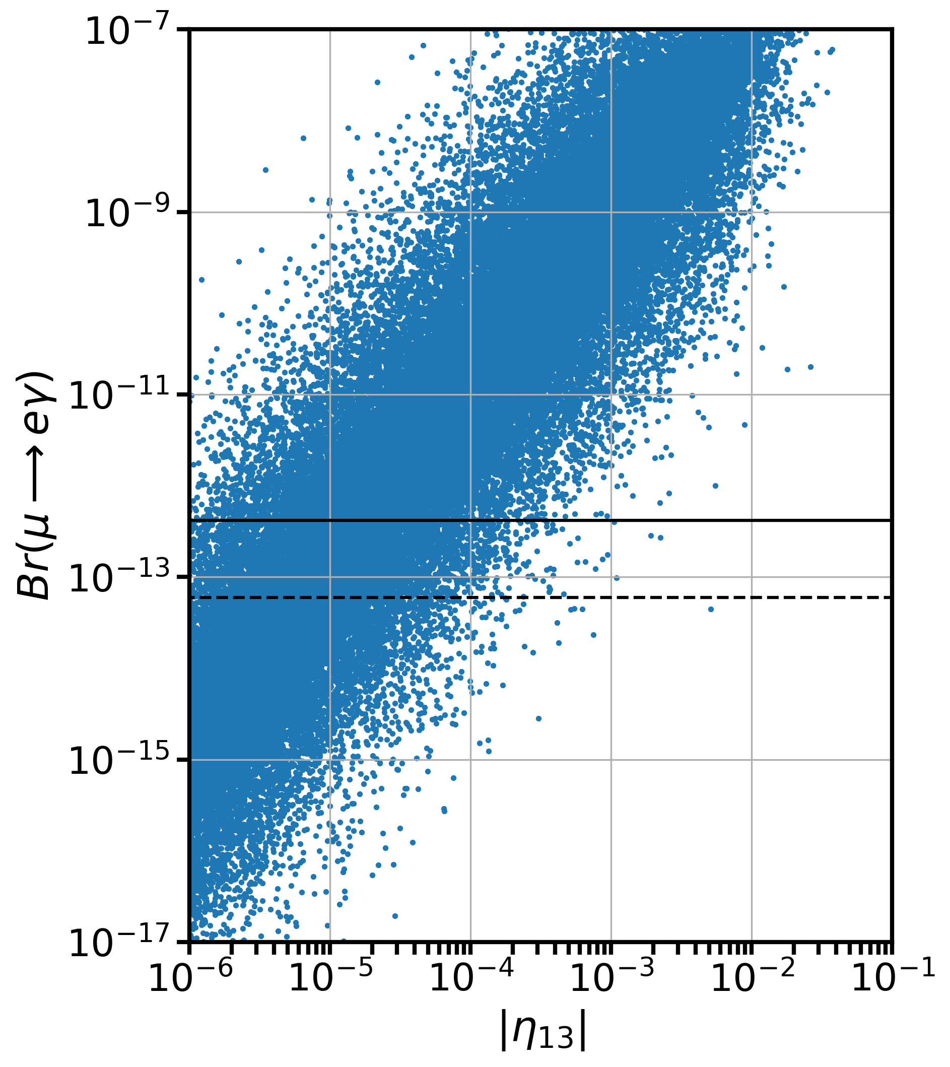
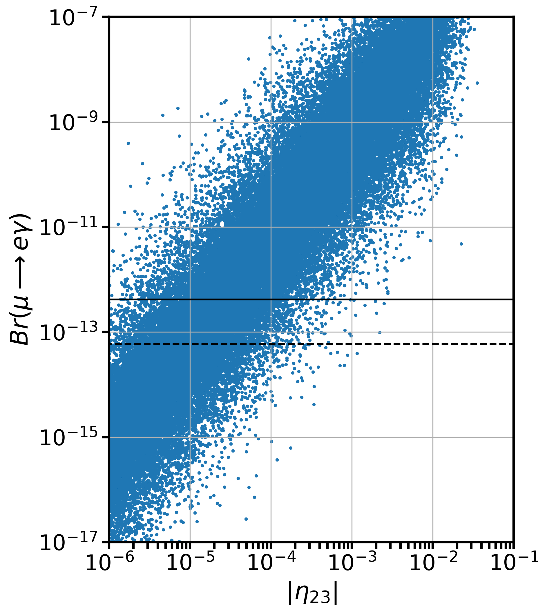
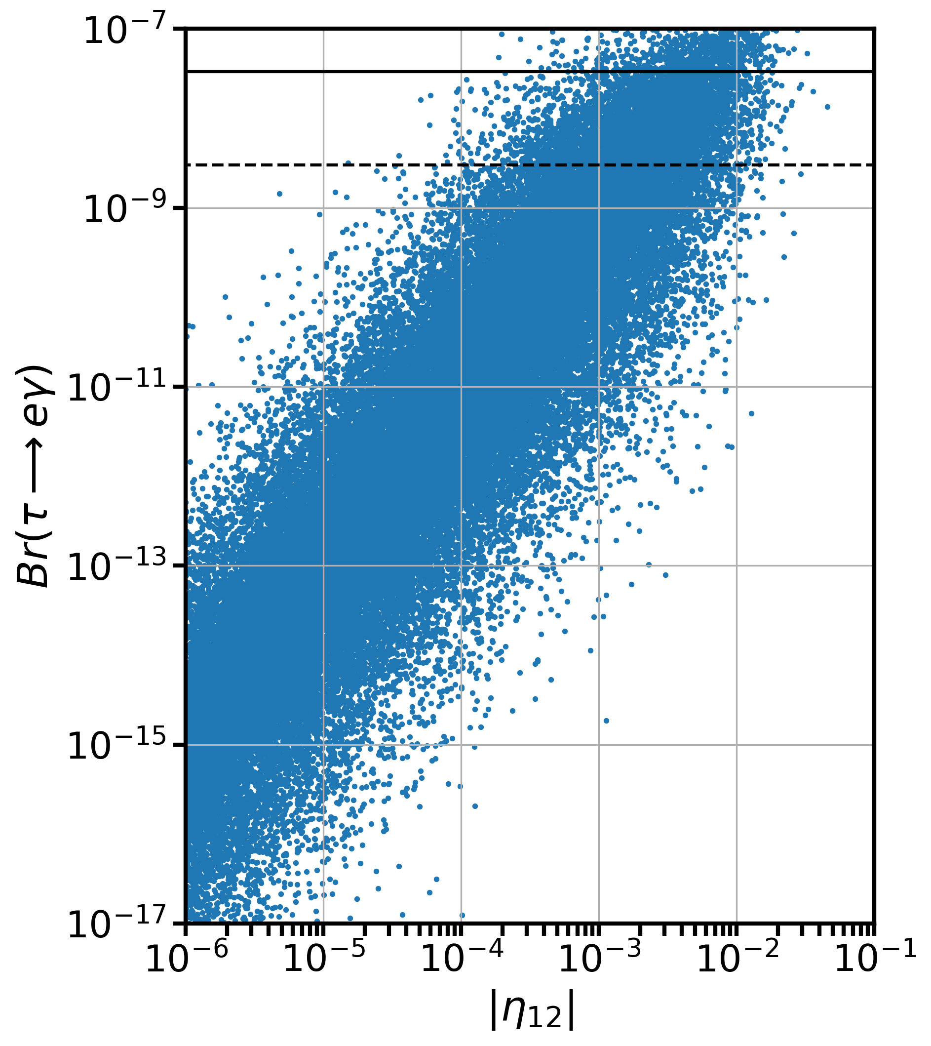
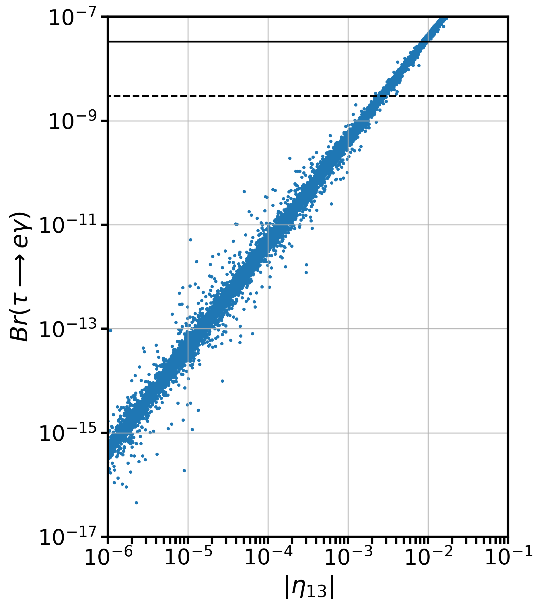
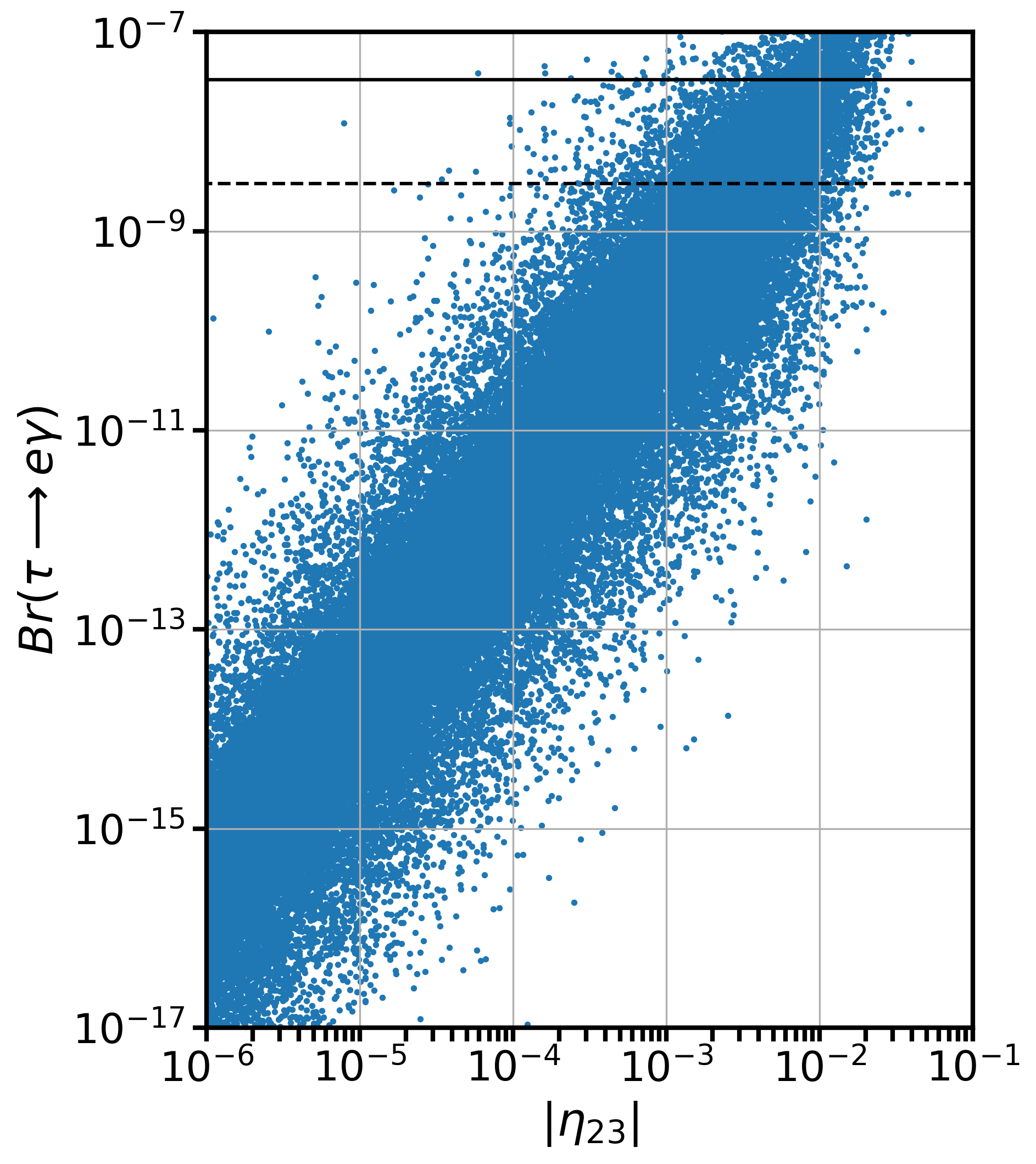
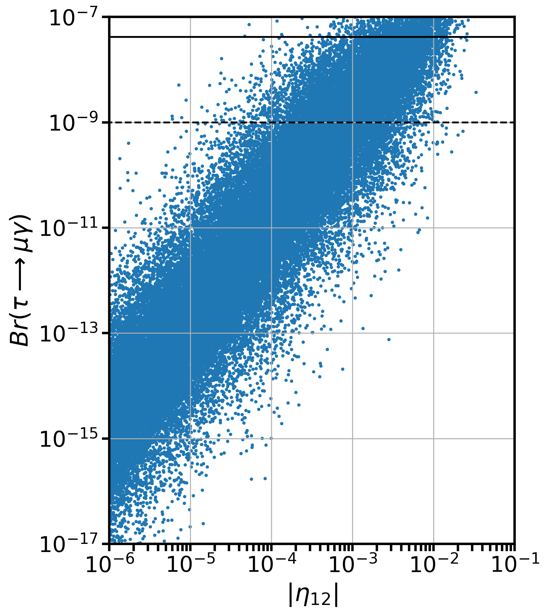
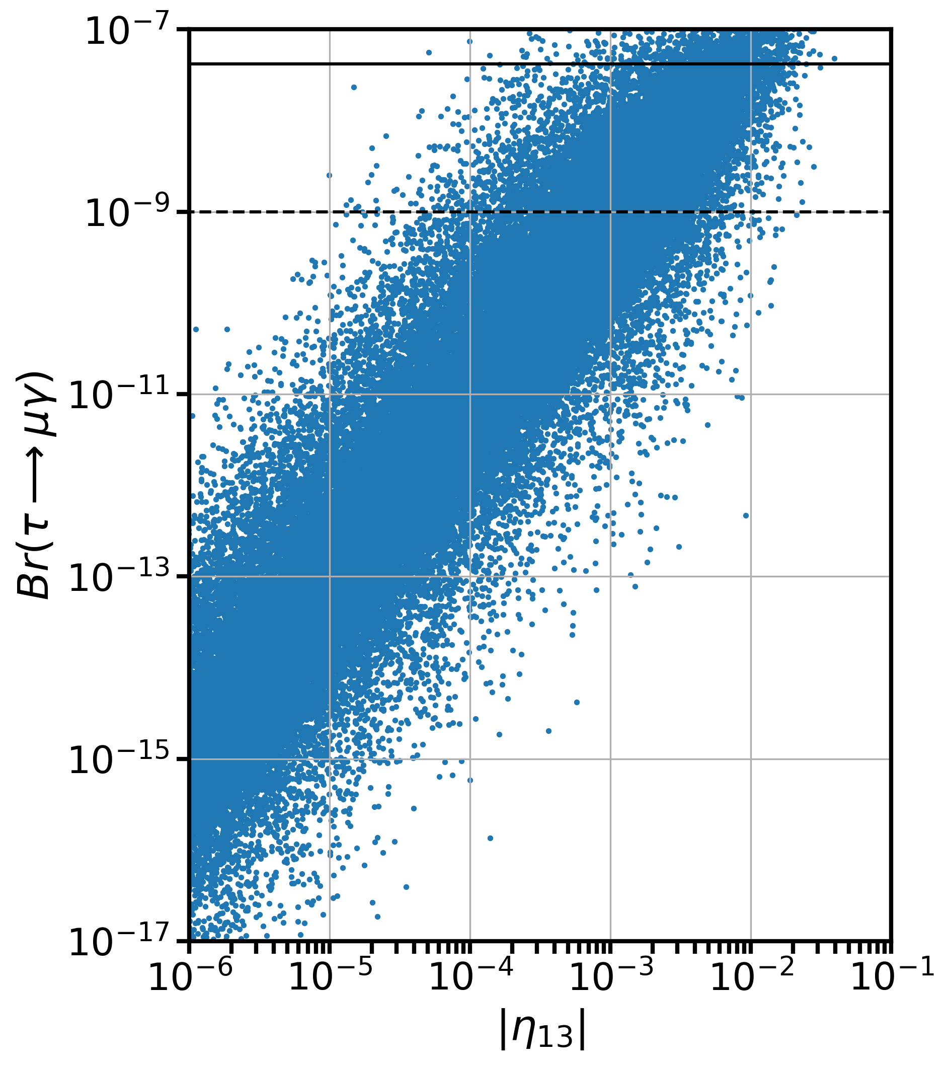
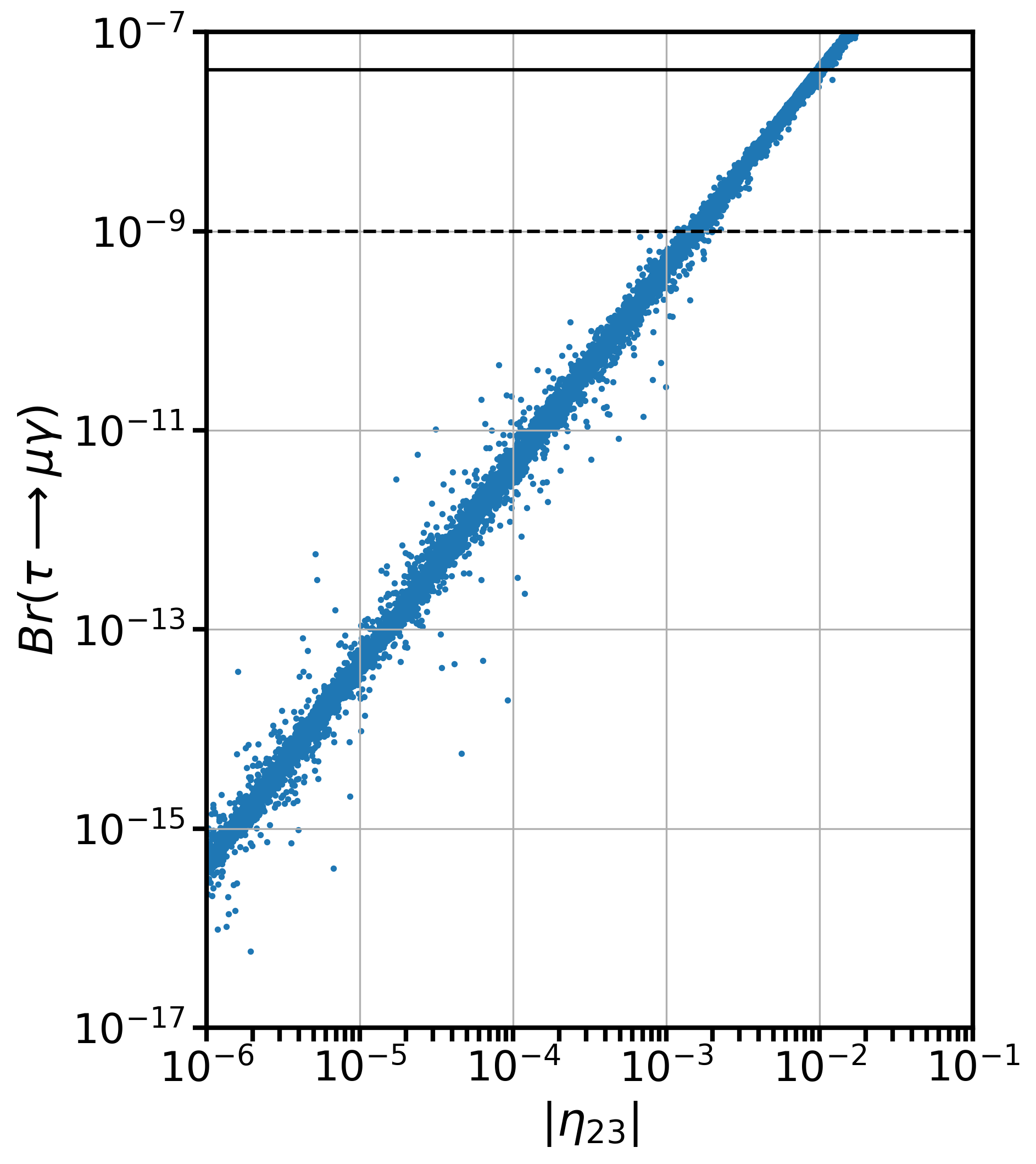
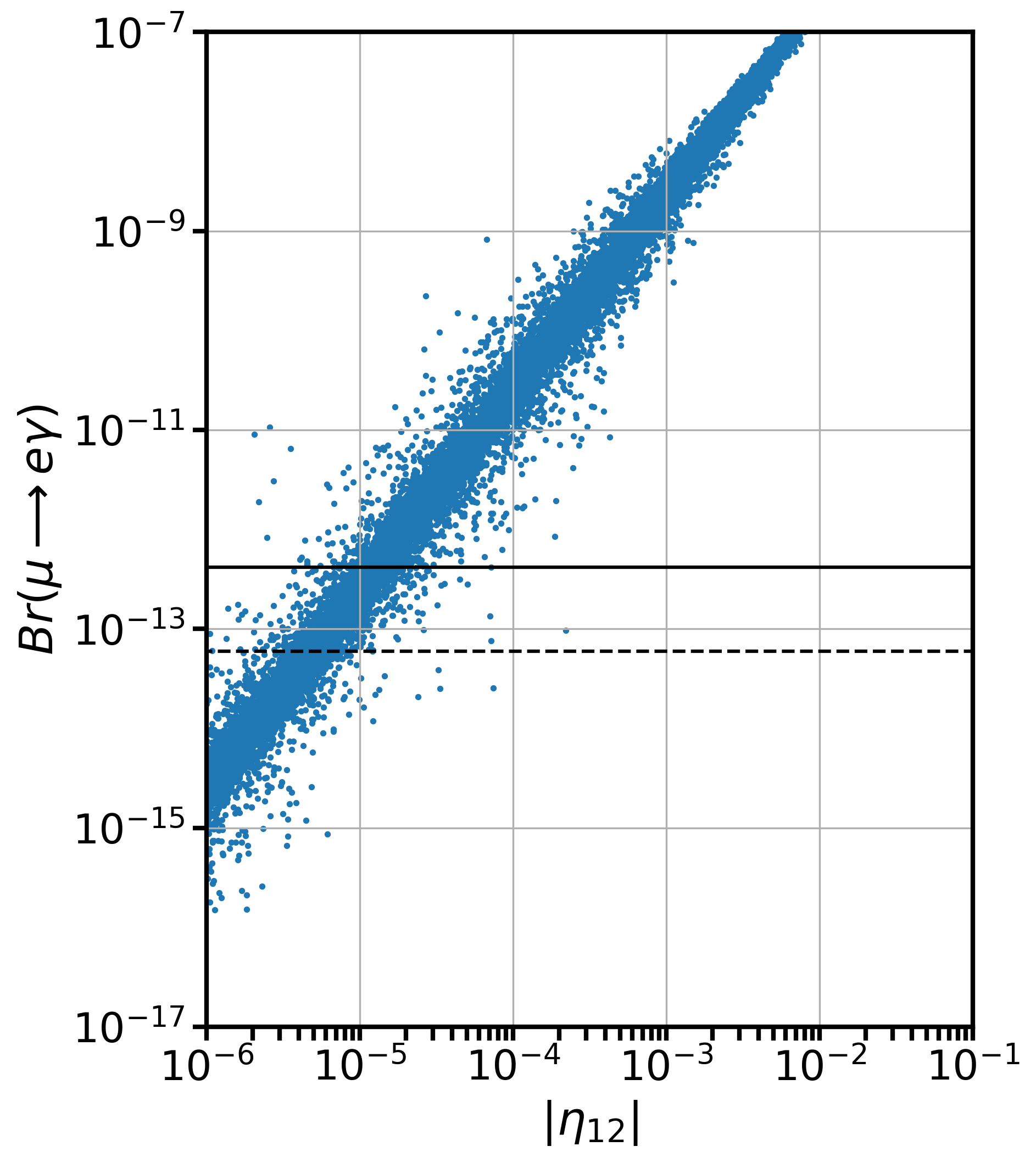
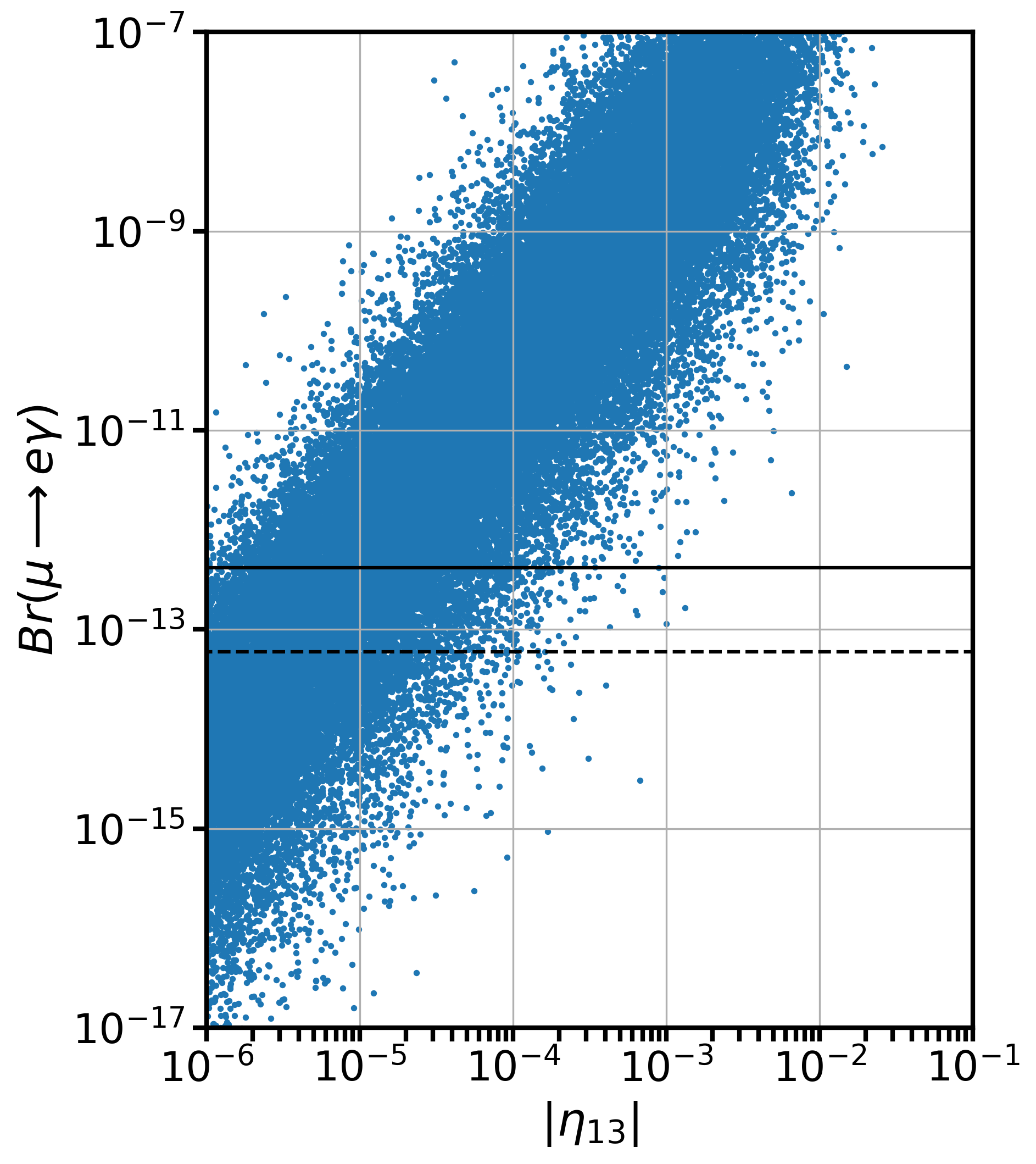
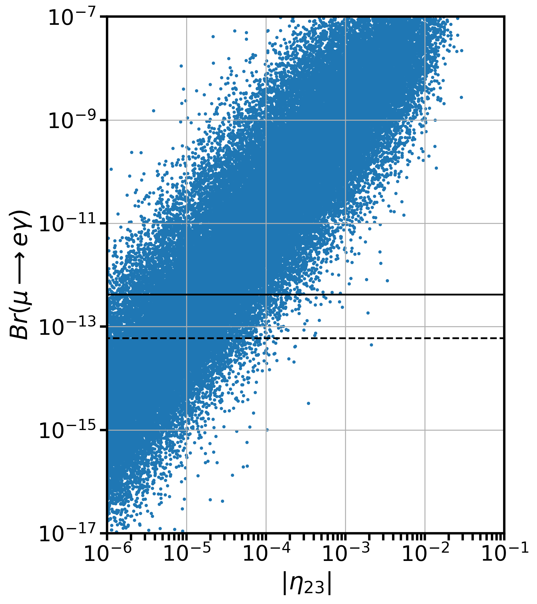
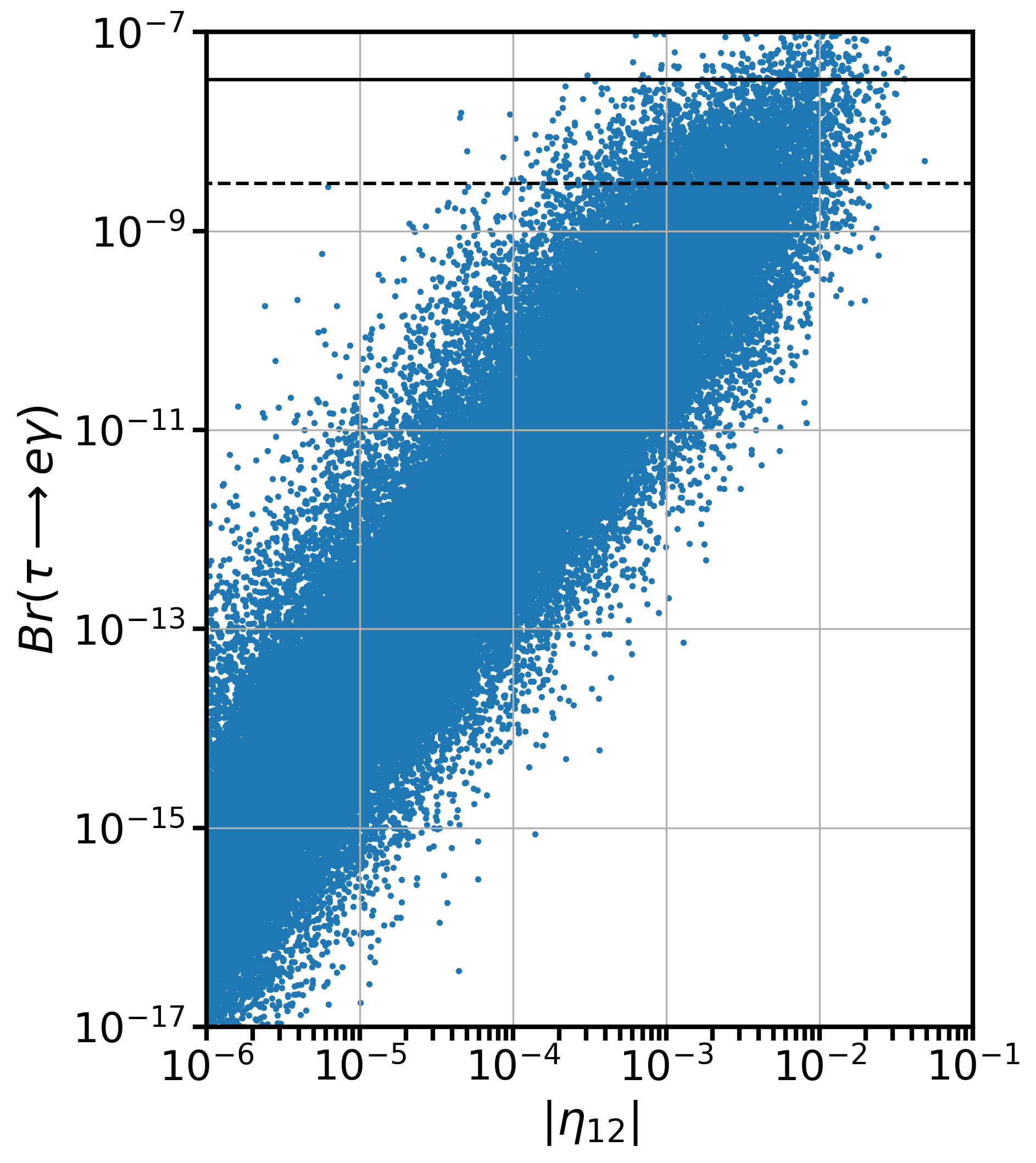
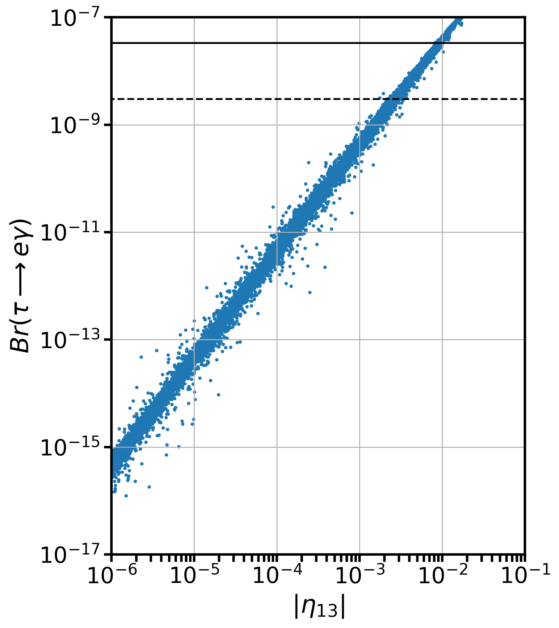
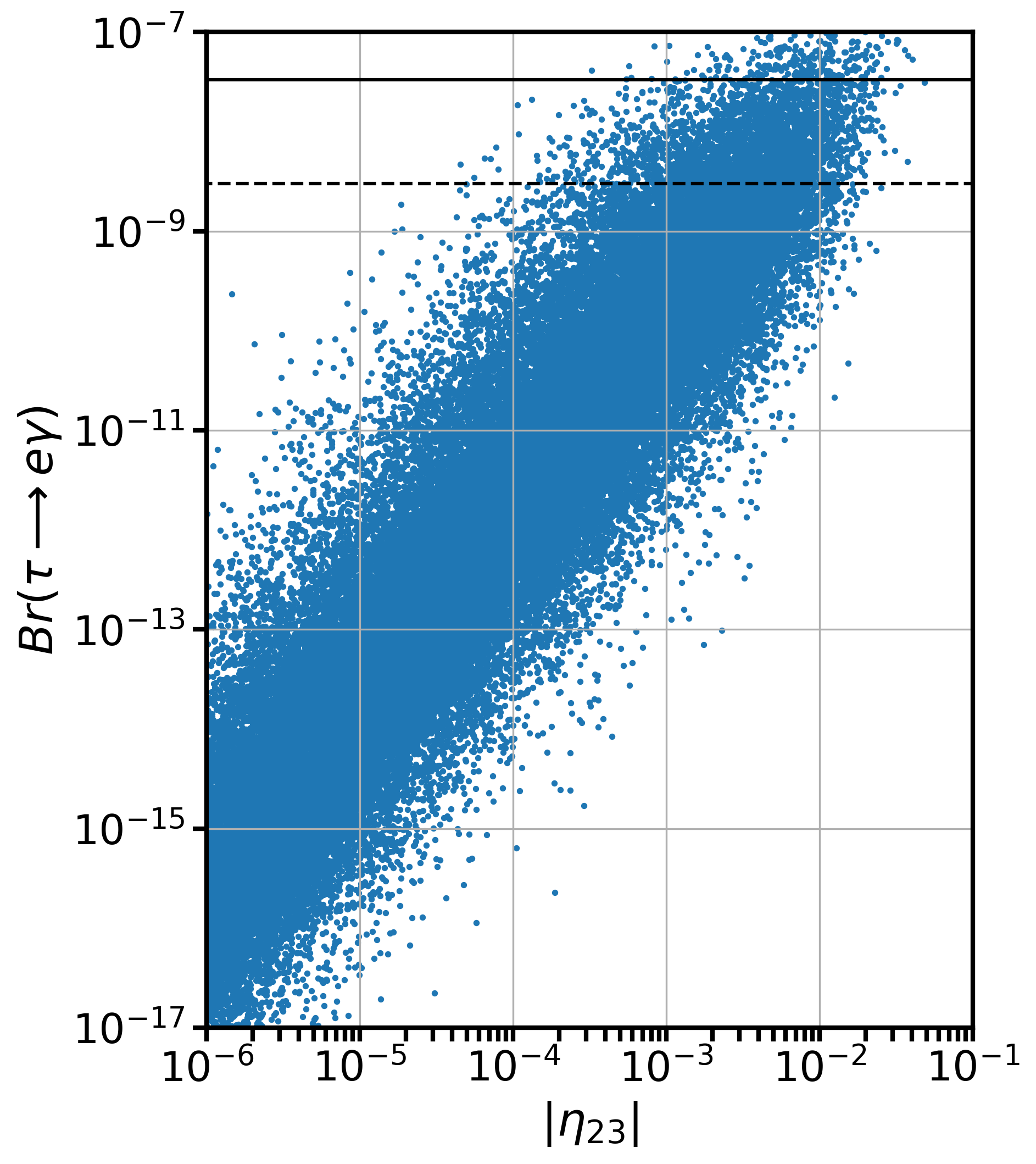
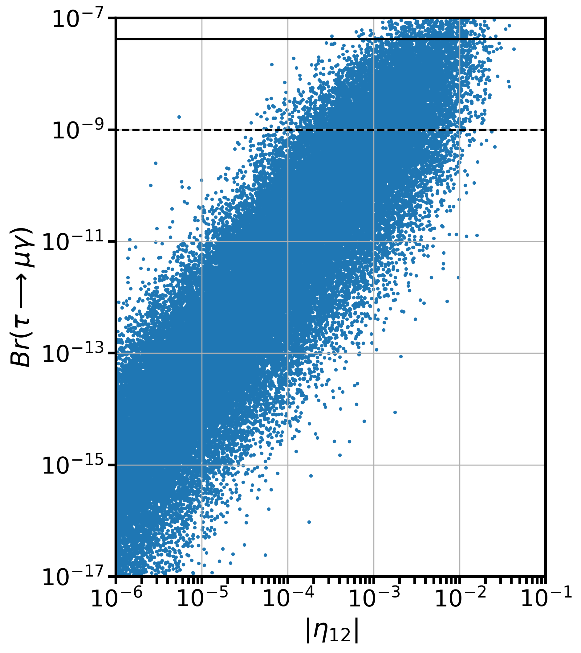
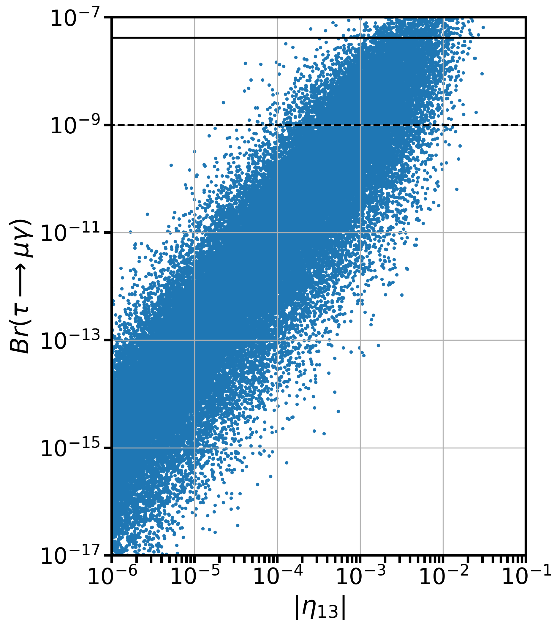
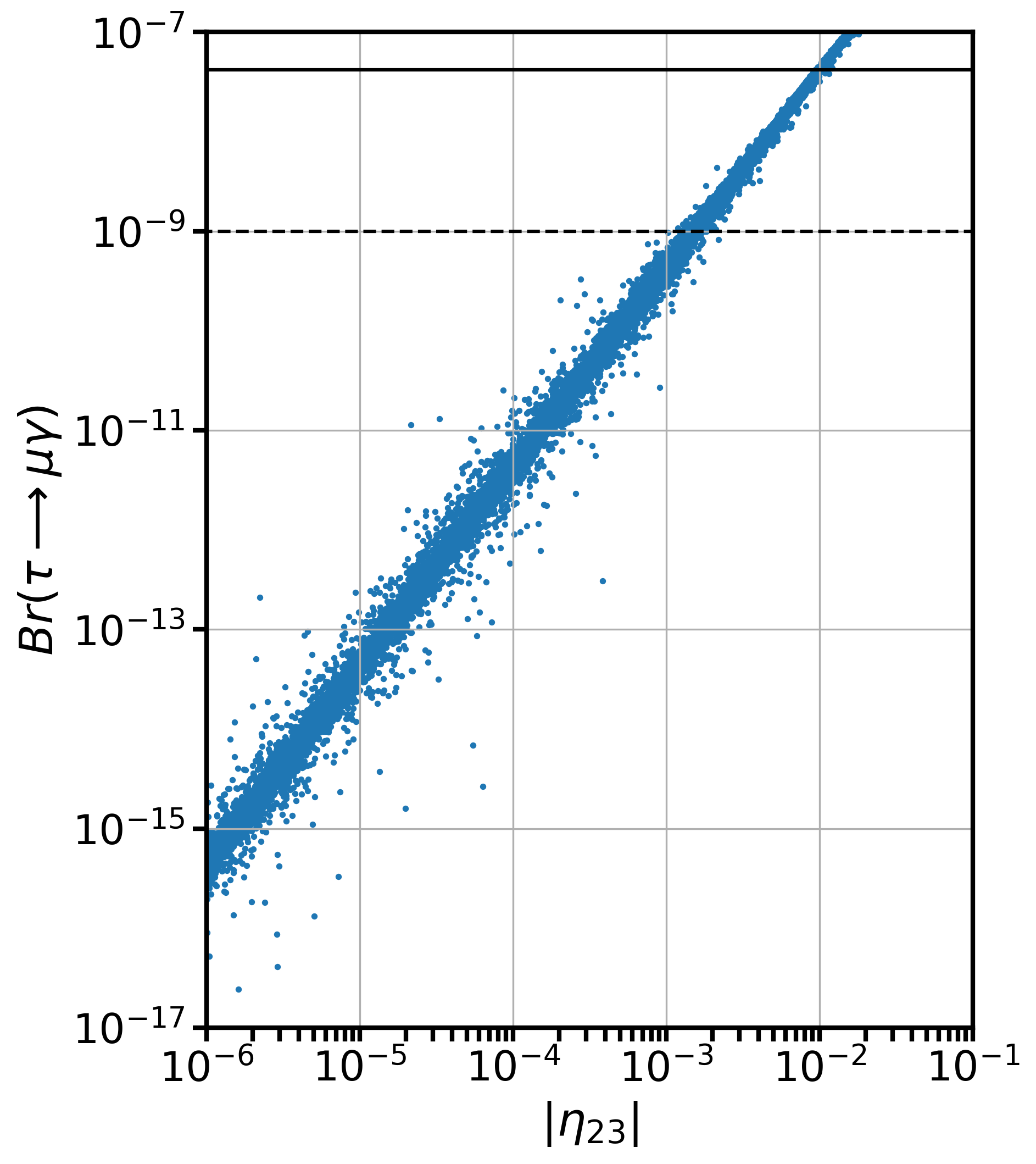
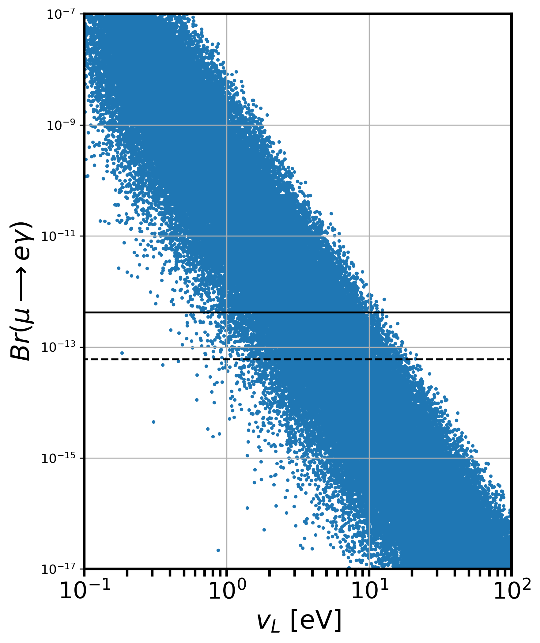
We perform a Monte Carlo analysis to find the current and future sensitivity to non-unitary parameters from cLFV processes. We showed our results in Figs.( 1-3), where we plotted the branching ratios of the cLFV processes versus the relevant parameters for the linear seesaw scheme. In Fig. 1, we ilustrate the constraints on $v_{L}$ using the cLFV process. We can see from this plot that the constraint on the $v_{L}$ parameter, that gives us the scale of the $M_{L}$ matrix, is around 10 eVs. On other hand, we have also computed the Monte Carlo analysis for the cLFV in terms of the non-unitary parameters. In particular, we have computed the branching ratios for the $\mu\to e\gamma$, $\tau\to e\gamma$, and $\tau\to\mu\gamma$ depending on the non-unitary parameters $|\eta_{12}|$, $|\eta_{13}|$, and $|\eta_{23}|$. The results, for normal ordering (NO), are shown in Fig. (2), where we show the current constraint for each process (Refs. [32, 35]) with a solid horizontal line and the future expected constraint [32, 34] with a dashed line. We can see from these plots that the most restrictive constraints come from the $\mu\to e\gamma$ while the other two decays give mild contraints in comparison with the first one. We collect the current and expected future sensitivities for this NO case in Table 3. For the Inverted Ordering case (IO), we show the equivalent results in Fig. (3). Again, we show the current and future expected sensitivities in Table 4. As in the previous case, fot this IO we also find that the $\mu\to e\gamma$ results give the most restrictive current constraints and it is expected that will lead the constraining power in the future. We can notice that the results are similar for both normal and inverted mass ordering, except for the $|\eta_{23}|$ parameter, that is more restricted for the inverted ordering case. Finally, for the sake of completeness and using Eq. (37), we show the non-unitary sensitivity in terms of the $\alpha$ parametrization in Table 5.

In summary, we studied non-unitary signatures of the Linear Seesaw model in charged lepton flavor violation processes. For this analysis, we used the current constraints on the oscillation parameters (for normal and inverted ordering) and on the lightest mass $m_{1}$ given by cosmological constraints. We use the Casas-Ibarra parametrization to compute numerically the $M_{D}$ entrances in terms of the $M$ and $M_{L}$ matrix values. In order to make our results comparable with analysis from different observables, we wrote explicitly the relation between the so-called $\eta$ and $\alpha$ parameterizations that came from Eq. (37) ($\eta_{ij}=\frac{1}{2}\alpha_{ij}$). We can compare the current constraints for the $\alpha$ parameters [24] with the constraints that we acquired from our analysis, which is given in terms of $\eta$ parameters. We found that the constraints coming from the $\mu\longrightarrow e\gamma$ process are more sensitive than the current oscillation experimental constraints and the other two processes give us a competitive sensitivity compared with the current limits.

Parameters	$\mu\longrightarrow e\gamma$		$\tau\longrightarrow e\gamma$		$\tau\longrightarrow\mu\gamma$
	Current	Future	Current	Future	Current	Future
$|\eta_{12}|\lessapprox$	$2\times 10^{-5}$	$10^{-5}$	$2\times 10^{-2}$	$10^{-2}$	$2\times 10^{-2}$	$5\times 10^{-3}$
$|\eta_{13}|\lessapprox$	$2\times 10^{-4}$	$6\times 10^{-5}$	$10^{-2}$	$3\times 10^{-3}$	$2\times 10^{-2}$	$7\times 10^{-3}$
$|\eta_{23}|\lessapprox$	$4\times 10^{-4}$	$2\times 10^{-4}$	$3\times 10^{-2}$	$2\times 10^{-2}$	$10^{-2}$	$2\times 10^{-3}$

Table 3: The current and the future sensitivity for the non-unitary parameters from the different charged flavor violation processes in the normal ordering case.

Parameters	$\mu\longrightarrow e\gamma$		$\tau\longrightarrow e\gamma$		$\tau\longrightarrow\mu\gamma$
	Current	Future	Current	Future	Current	Future
$|\eta_{12}|\lessapprox$	$2\times 10^{-5}$	$10^{-5}$	$2\times 10^{-2}$	$10^{-2}$	$2\times 10^{-2}$	$10^{-2}$
$|\eta_{13}|\lessapprox$	$2\times 10^{-4}$	$6\times 10^{-5}$	$10^{-2}$	$3\times 10^{-3}$	$2\times 10^{-2}$	$7\times 10^{-3}$
$|\eta_{23}|\lessapprox$	$2\times 10^{-4}$	$7\times 10^{-5}$	$3\times 10^{-2}$	$2\times 10^{-2}$	$10^{-2}$	$2\times 10^{-3}$

Table 4: The current and the future sensitivity for the non-unitary parameters from the different charged flavor violation processes in the inverse ordering case.

Parameters	$\mu\longrightarrow e\gamma$		$\tau\longrightarrow e\gamma$		$\tau\longrightarrow\mu\gamma$
	Current	Future	Current	Future	Current	Future
$|\alpha_{12}|\lessapprox$	$4\times 10^{-5}$	$2\times 10^{-5}$	$4\times 10^{-2}$	$2\times 10^{-2}$	$4\times 10^{-2}$	$10^{-2}$
$|\alpha_{13}|\lessapprox$	$4\times 10^{-4}$	$1.2\times 10^{-4}$	$2\times 10^{-2}$	$6\times 10^{-3}$	$4\times 10^{-2}$	$1.4\times 10^{-2}$
$|\alpha_{23}|\lessapprox$	$8\times 10^{-4}$	$4\times 10^{-4}$	$6\times 10^{-2}$	$4\times 10^{-2}$	$2\times 10^{-2}$	$4\times 10^{-3}$

Table 5: The current and the future sensitivity for the $\alpha$ parameters from the different charged flavor violation processes in the normal ordering case.

V Acknowledgements

We thank Gerardo Hernández-Tomé and Eduardo Peinado for useful discussions. This work has been partially supported by CONAHCyT research grant: A1-S-23238. The work of O. G. M. has also been supported by SNII-Mexico.

References

- [1] Peter Minkowski. at a Rate of One Out of Muon Decays? Phys. Lett. B, 67:421–428, 1977.
- [2] Rabindra N. Mohapatra and Goran Senjanovic. Neutrino Mass and Spontaneous Parity Nonconservation. Phys. Rev. Lett., 44:912, 1980.
- [3] Murray Gell-Mann, Pierre Ramond, and Richard Slansky. Complex Spinors and Unified Theories. Conf. Proc. C, 790927:315–321, 1979.
- [4] Tsutomu Yanagida. Horizontal gauge symmetry and masses of neutrinos. Conf. Proc. C, 7902131:95–99, 1979.
- [5] J. Schechter and J. W. F. Valle. Neutrino Masses in SU(2) x U(1) Theories. Phys. Rev. D, 22:2227, 1980.
- [6] Robert Foot, H. Lew, X. G. He, and Girish C. Joshi. Seesaw Neutrino Masses Induced by a Triplet of Leptons. Z. Phys. C, 44:441, 1989.
- [7] R. N. Mohapatra and J. W. F. Valle. Neutrino Mass and Baryon Number Nonconservation in Superstring Models. Phys. Rev. D, 34:1642, 1986.
- [8] Evgeny K. Akhmedov, Manfred Lindner, Erhard Schnapka, and J. W. F. Valle. Dynamical left-right symmetry breaking. Phys. Rev. D, 53:2752–2780, 1996.
- [9] Michal Malinsky, J. C. Romao, and J. W. F. Valle. Novel supersymmetric SO(10) seesaw mechanism. Phys. Rev. Lett., 95:161801, 2005.
- [10] Aditya Batra, Praveen Bharadwaj, Sanjoy Mandal, Rahul Srivastava, and José W. F. Valle. Phenomenology of the simplest linear seesaw mechanism. JHEP, 07:221, 2023.
- [11] O. G. Miranda, D. K. Papoulias, O. Sanders, M. Tórtola, and J. W. F. Valle. Future CEvNS experiments as probes of lepton unitarity and light-sterile neutrinos. Phys. Rev. D, 102:113014, 2020.
- [12] F. J. Escrihuela, D. V. Forero, O. G. Miranda, M. Tortola, and J. W. F. Valle. On the description of nonunitary neutrino mixing. Phys. Rev. D, 92(5):053009, 2015. [Erratum: Phys.Rev.D 93, 119905 (2016)].
- [13] Salvador Centelles Chuliá, Antonio Herrero-Brocal, and Avelino Vicente. The Type-I Seesaw family. 4 2024.
- [14] J. C. Garnica, G. Hernández-Tomé, and E. Peinado. Charged lepton-flavor violating processes and suppression of nonunitary mixing effects in low-scale seesaw models. Phys. Rev. D, 108(3):035033, 2023.
- [15] D. V. Forero, S. Morisi, M. Tortola, and J. W. F. Valle. Lepton flavor violation and non-unitary lepton mixing in low-scale type-I seesaw. JHEP, 09:142, 2011.
- [16] Kazuyuki Kanaya. Neutrino Mixing in the Minimal SO(10) Model. Prog. Theor. Phys., 64:2278, 1980.
- [17] J. Schechter and J. W. F. Valle. Neutrino Decay and Spontaneous Violation of Lepton Number. Phys. Rev. D, 25:774, 1982.
- [18] Michael Gronau, Chung Ngoc Leung, and Jonathan L. Rosner. Extending Limits on Neutral Heavy Leptons. Phys. Rev. D, 29:2539, 1984.
- [19] Enrico Nardi, Esteban Roulet, and Daniele Tommasini. Limits on neutrino mixing with new heavy particles. Phys. Lett. B, 327:319–326, 1994.
- [20] Anupama Atre, Tao Han, Silvia Pascoli, and Bin Zhang. The Search for Heavy Majorana Neutrinos. JHEP, 05:030, 2009.
- [21] F. J. Escrihuela, D. V. Forero, O. G. Miranda, M. Tórtola, and J. W. F. Valle. Probing CP violation with non-unitary mixing in long-baseline neutrino oscillation experiments: DUNE as a case study. New J. Phys., 19(9):093005, 2017.
- [22] Enrique Fernandez-Martinez, Josu Hernandez-Garcia, and Jacobo Lopez-Pavon. Global constraints on heavy neutrino mixing. JHEP, 08:033, 2016.
- [23] Mattias Blennow, Enrique Fernández-Martínez, Josu Hernández-García, Jacobo López-Pavón, Xabier Marcano, and Daniel Naredo-Tuero. Bounds on lepton non-unitarity and heavy neutrino mixing. JHEP, 08:030, 2023.
- [24] D. V. Forero, C. Giunti, C. A. Ternes, and M. Tortola. Nonunitary neutrino mixing in short and long-baseline experiments. Phys. Rev. D, 104(7):075030, 2021.
- [25] Peter B. Denton and Julia Gehrlein. New oscillation and scattering constraints on the tau row matrix elements without assuming unitarity. Journal of High Energy Physics, 2022(6), jun 2022.
- [26] Debajyoti Dutta and Samiran Roy. Non-Unitarity at DUNE and T2HK with Charged and Neutral Current Measurements. J. Phys. G, 48(4):045004, 2021.
- [27] Sabya Sachi Chatterjee, O. G. Miranda, M. Tórtola, and J. W. F. Valle. Nonunitarity of the lepton mixing matrix at the European Spallation Source. Phys. Rev. D, 106(7):075016, 2022.
- [28] Jesús Miguel Celestino-Ramírez, F. J. Escrihuela, L. J. Flores, and O. G. Miranda. Testing the nonunitarity of the leptonic mixing matrix at FASERv and FASERv2. Phys. Rev. D, 109(1):L011705, 2024.
- [29] Salvador Centelles Chuliá, Omar Miranda, and Jose W. F. Valle. Leptonic neutral-current probes in a short-distance DUNE-like setup. 1 2024.
- [30] Mattias Blennow, Pilar Coloma, Enrique Fernandez-Martinez, Josu Hernandez-Garcia, and Jacobo Lopez-Pavon. Non-Unitarity, sterile neutrinos, and Non-Standard neutrino Interactions. JHEP, 04:153, 2017.
- [31] Bo He, T. P. Cheng, and Ling-Fong Li. A Less suppressed mu — e gamma loop amplitude and extra dimension theories. Phys. Lett. B, 553:277–283, 2003.
- [32] J. Adam et al. New constraint on the existence of the decay. Phys. Rev. Lett., 110:201801, 2013.
- [33] A. M. Baldini et al. The design of the MEG II experiment. Eur. Phys. J. C, 78(5):380, 2018.
- [34] Bernard Aubert et al. Searches for Lepton Flavor Violation in the Decays tau+- — e+- gamma and tau+- — mu+- gamma. Phys. Rev. Lett., 104:021802, 2010.
- [35] W. Altmannshofer et al. The Belle II Physics Book. PTEP, 2019(12):123C01, 2019. [Erratum: PTEP 2020, 029201 (2020)].
- [36] G. D’Ambrosio, G. F. Giudice, G. Isidori, and A. Strumia. Minimal flavor violation: An Effective field theory approach. Nucl. Phys. B, 645:155–187, 2002.
- [37] J. A. Casas and A. Ibarra. Oscillating neutrinos and . Nucl. Phys. B, 618:171–204, 2001.
- [38] P. F. de Salas, D. V. Forero, S. Gariazzo, P. Martínez-Miravé, O. Mena, C. A. Ternes, M. Tórtola, and J. W. F. Valle. 2020 global reassessment of the neutrino oscillation picture. JHEP, 02:071, 2021.