Quantum fluctuation theorem in a curved spacetime
Abstract
The interplay between thermodynamics, general relativity and quantum mechanics has long intrigued researchers. Recently, important advances have been obtained in thermodynamics, mainly regarding its application to the quantum domain through fluctuation theorems. In this letter, we apply Fermi normal coordinates to report a fully general relativistic detailed quantum fluctuation theorem based on the two point measurement scheme. We demonstrate how the spacetime curvature can produce entropy in a localized quantum system moving in a general spacetime. The example of a quantum harmonic oscillator living in an expanding universe is presented. This result implies that entropy production is strongly observer dependent and deeply connects the arrow of time with the causal structure of the spacetime.
Introduction. Although the fundamental laws of Nature respect the time-reverse symmetry, irreversible processes are everywhere in the natural world [1]. Irreversibility, marked by the production of thermodynamic entropy [2], establishes the thermodynamic arrow of time, pointing from low to high entropy [3]. A significant step in this research area has been the formulation of fluctuation theorems, which extend the second law of thermodynamics. These theorems assert that the likelihood of observing a negative entropy production, or a reversal of the arrow of time, vanishes exponentially [4, 5, 6, 7, 8]. One implication of these findings is that, on average, a positive entropy production will be typically manifested in any given process.
On the other hand, the intersection of relativity and thermodynamics dates back to over a century ago, with Einstein and Planck delving into how thermodynamic properties, such as temperature, behaves under the change in reference frames [9, 10, 11]. A remarkable advance in this intersection involves the development of black hole thermodynamics [12], which was subsequently used to demonstrate that Einstein’s field equations can be interpreted as a thermodynamic equation of state [13]. This approach has been further applied to investigate the non-equilibrium properties of spacetime [14]. Moreover, attempts for building a statistical mechanical theory of the gravitational field, alongside the suggestion that time may have a thermodynamic origin, was made in Refs. [17, 18, 15, 16]. Lately, there have been advancements in extending thermodynamic relations to Quantum Field Theory (QFT). In particular, the Jarzynski equality was established for QFT within a flat spacetime, employing both direct two-point and indirect measurements [19, 20].
Here, by working in this intersection, we demonstrate how the spacetime curvature can produce entropy in a localized quantum system that moves in a general spacetime. Some developments in this direction have been achieved. In the realm of linear effects, Mottola [21] established a fluctuation-dissipation relation in curved spacetime. Iso et al. [22] explored the non-equilibrium fluctuations of a black hole horizon through the application of the Jarzynski equality [23] along with the generalized second law of thermodynamics [24]. Moreover, a fluctuation theorem for a quantum field in a specific model of an expanding Universe was described in Ref. [25].
Our central result goes beyond these studies, by proving a fully general relativistic quantum fluctuation theorem, based on the two point measurement (TPM) scheme [7], for a localized quantum system, extending the findings of Ref. [26] in two significant ways. Firstly, the Tasaki-Crooks theorem entails the Jarzynski equality when integrated across the probability distribution. Secondly, and most notably, it unveils the complete impact of the gravitational field on irreversible processes by explicitly considering the effect of spacetime curvature. Moreover, our primary finding is illustrated by investigating a quantum mechanical harmonic oscillator living in an expanding universe. The main implications of our result are discussed in the end of this letter.
We use natural units in which the speed of light , Planck’s constant , Newton’s gravitational constant and Boltzmann constant are set to unity. The signature of the metric is with Greek letter running from to , while the Latin letters runs from to with exception for the letters and that runs from to . is the Minkowski metric.
Fermi normal coordinates. We consider the stochastic thermodynamics of a non-relativistic quantum system that is localized around a time-like trajectory in an arbitrary spacetime. In order to define physical quantities, we employ Fermi normal coordinates [27]. This choice is based on the fact that such coordinates properly define rest spaces where the Hilbert space of the quantum system can be constructed and all the relevant quantities can be unambiguously defined. Also, using the Fermi transport, it is possible to follow the evolution of the system from one of the rest space to the others. This will be fundamental for us to define thermodynamic variables and processes.
Our strategy is the following. We first build the Fermi normal coordinates around a time-like trajectory that describes the worldline of our laboratory frame. Then, we consider the Hamiltonian formulation of the dynamics of a localized quantum particle around this time-like trajectory [28, 29, 30]. This will provide the necessary description of a localized quantum system in a curve spacetime, which is the basic ingredient employed in order to prove our main result: the quantum detailed fluctuation theorem on a curved spacetime.
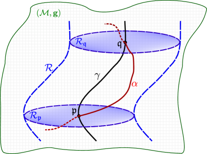
Technically, we consider a four-dimensional spacetime , with being a differentiable manifold while stands for a Lorentzian metric. The world-line of the laboratory frame is a time-like curve , which can be parameterized by its proper time . The frame -velocity fulfils .
The next step is to build the Fermi normal coordinates, which are constructed as follows (see Appendix A for details). First, we define as the time component of such coordinate system. An orthonormal basis is then defined at a point , where labels the four basis vector while is identified with the tangent vector . Thus, at point we have . Now we extend this frame along the trajectory such that the basis remains orthogonal. This is achieved by transporting the vectors via the Fermi-Walker transport [31].
By considering the normal neighbourhood of the point we can construct the space-like Fermi normal coordinates. From this, we define the local rest space of the point as the set of points spanned by all geodesics that start from with tangent vector orthogonal to . Therefore, the coordinates can be assigned to any point . Finally, the local rest space of the curve is defined as which can be seen as a local foliation of the spacetime around the curve such that any point in is described by the Fermi normal coordinates . See Appendix A for more details.
The system Hamiltonian. We need to define the Hamiltonian of our system, which will be constructed around the time-like trajectory employing the Fermi normal coordinates. It is worth mentioning that Ref. [28] provides a formal and elegant description of a localized quantum system in a curved spacetime using the Fermi normal coordinates. However, our construction is also related to the formulation reported in Refs. [29, 30], where a structured quantum system was considered. We present here only an overview of the calculations, while the details are explicitly given in Appendix B.
We consider a particle travelling along the world-line around the trajectory of the laboratory frame, i.e., the time-like curve is contained in the local rest space of the curve , where the Fermi normal coordinates are valid. See the sketch in Fig. 1.
Considering a non-relativistic system (the particle’s internal and kinetic energies are much smaller than its rest energy), we can write the Hamiltonian to the lowest order as
| (1) |
where
| (2) |
is directly related to the time dilation factor between the proper time of the laboratory frame and the proper time of the system (or the comoving observer). Besides, and are the components, in the Fermi normal coordinates, of the -acceleration and the Riemann curvature tensor, respectively, evaluated at point . Finally, is the square of the momentum of the particle. In addition, is the Hamiltonian of the centre-of-mass, which is given by
| (3) |
We can interpret the last two terms of Eq. (3) as perturbations to the (flat space-time) free Hamiltonian .
We now have all the necessary ingredients to present our main result, a detailed fluctuation theorem obeyed by the described system.
Fluctuation theorem. We start by describing the protocol employed to derive the detailed fluctuation theorem under the TPM scheme for a localized quantum system in a curved spacetime, thus going far beyond Ref. [26] in two important ways. First, here we provide a detailed fluctuation theorem, while in Ref. [26] just the integral one is presented. Secondly, and most important, here we uncover the full role played by the gravitational field in irreversible phenomena, by taking into account the effect of spacetime curvature explicitly.
Let us first recall that a spacetime is time-orientable if a continuous designation of future-directed and past-directed for time-like vectors can be made over the entire manifold [32]. In our case, we only assume that at least a portion of the spacetime is time orientable, i.e., that the local rest space of the curve is time-orientable. This can be done since we are assuming that the curve is time-like and describes the world-line of the laboratory frame. Moreover, we assume that the curve is oriented towards the future. In addition, from the curve and its local rest space , it was possible to obtain the Hamiltonian (1) that governs the evolution of our system and therefore defines a notion of time flow in the sense defined by Connes and Rovelli [18]. This demand is necessary for defining local thermal equilibrium states [26, 18, 15, 16].
We define two protocols, one in the forward direction of time and the other one in the backwards direction of time. The distinguishability of these processes will be employed as a measure of irreversibility of the forward process [4]. Both processes consist in preparing the system in an equilibrium state, measuring its energy, letting it evolve under a certain quantum map and measuring its final energy. From the results of these measurements, entropy production can be defined. We define both processes in the sequence.
The forward process is defined as follows. As depicted in Fig. 1, at point , the curves and intersect and the observer (in the laboratory frame) performs the first projective measurement in the energy eigenbasis. To do this, we first suppose that the state of our system is given by , with representing the state of the external degrees of freedom while the internal degrees of freedom are described by the thermal state with and being the initial Hamiltonian of the internal degrees of freedom and the partition function, respectively. is the inverse temperature, which can be properly defined in the present setup [26]. The measurement is performed in the eigenbasis of at point , resulting in the energy eigenvalue with probability . After this measurement, the state of our system is given by . Then, as the quantum system travels along its world line , its evolution, with respect to the laboratory frame, is governed by Hamiltonian (1) and can be written as
where is the time-ordering operator and . The last equality follows from the semiclassical approximation, in which the motion of the quantum particle along its world-line is well-defined. Hence, the internal state evolves accordingly to .
At some latter proper time, when the system intersects again the laboratory frame at the point , as depicted in Fig 1, the last step of the forward process is realized by a projective measurement with respect to the internal Hamiltonian , with , . Hence, from the definition of work as the stochastic variable , we can construct the work probability distribution density of the forward process as , where is the joint probability of obtaining in the first measurement and in the second one. It follows that
| (4) |
In order to define the reverse process, let us remember that, given a time orientation in a portion of the spacetime as the region , general relativity does not forbid us to define past-directed curves in [32]. For instance, given that the curves and parameterized by in Fig 1 are directed to the future, then we can obtain past-directed curves and by making . Hence, by following Ref. [8], the reverse process is defined as follows. At the point , the curves and intersect and a first projective measurement in the energy eigenbasis is realized in the laboratory frame. To do this, we first suppose that the state of our system is given by , where is the anti-unitary time-reversal operator [33], is the state of the external degrees of freedom, while the internal degrees of freedom are described by the thermal state . The next step of the reverse process consists in a measurement in the eigenbasis of at point , resulting in the energy eigenvalue with probability .
The time-reversal evolution of internal degrees of freedom is then governed by the micro-reversibility principle, i.e., , which holds under the assumption that the Hamiltonian (1) is invariant under time-reversal [8]. When the system intersects the laboratory frame at point , the final step of the reverse process is realized by a projective measurement with respect to the internal Hamiltonian . Hence, we can compute the work probability distribution density of the reverse process as
| (5) |
By using the fact that and where is the difference in the free energy, we obtain
| (6) |
This is the main result of the present paper, the quantum fluctuation theorem in a curved spacetime. It shows that a positive entropy production will be observed, on average, every time we are able to distinguish between the process and its time reversal.
Moreover, by integrating Eq. (6) over the probability distributions, we obtain the integral fluctuation theorem
| (7) |
which consists in the relativistic version of the Jarzynski equality. The subscript in the average above remembers us that the joint probability distribution depends on the path the system follows on the spacetime, while the subscript remember us that depends on the acceleration of the curve and the components of the curvature tensor evaluated at the curve . Another point is that the final temperature remains identical to the initial one, since it serves merely as a reference state established by the observer at the onset of the process. Therefore, our inquiry revolves around the extent to which the system deviates from this initial equilibrium state during its travel along its path in a curved spacetime. The answer to this question is precisely Eq. (7).
Some comments about particular realizations of our result are needed. First, if depends on , the results given by Eqs. (6) and (7) remains valid with the difference that we also have the contribution of the driven part of the Hamiltonian, thus modifying the entropy production rate. Second, disregarding the internal degrees of freedom, we can also derive Eq. (7) for the centre-of-mass degrees of freedom by considering localized quantum system within the local rest space of the curve . This is the case of the example discussed in the following. The total Hamiltonian is given by where is the non-perturbative Hamiltonian (or the Hamiltonian in flat space-time) with being the potential energy operator. Therefore, the terms and can be treated in the context of quantum mechanical perturbation theory with the spatial Fermi normal coordinates being position operators and the projective energy measurements are realized with regard to the Hamiltonian .
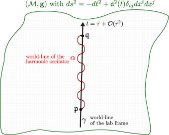
The expanding Universe. We illustrate our results considering a quantum mechanical harmonic oscillator (QHO) in an expanding universe described by the Friedmann-Robertson-Walker (FRW) metric [32]. The detailed calculations and a more in depth discussion can be found in Appendix C.
By taking the worldline of our laboratory frame as the one of the comoving observers —with the expansion of the universe— the FRW metric takes, in the Fermi normal coordinate system, the form
| (8) | |||||
with being the scale factor.
The system is initially prepared in a thermal state with inverse temperature and associated with the initial Hamiltonian whose spectrum is , with being a non-negative integer. After the first energy measurement, the system is let to evolve under the Hamiltonian
| (9) |
where the last term of Eq. (9) plays the role of a time-dependent external potential. Hence, we can interpret the non-stationary spacetime as the external force driving the quantum system out of equilibrium, which is the origin of the entropy production due to the dynamic nature of the spacetime.
In particular, let us restrict ourselves to the de-Sitter solution with the universe dominated only by a positive cosmological constant , which is a model both for the primordial inflationary phase and the current exponential expansion of our universe, i.e., the matter-energy content of the universe is described by a vacuum with positive energy density which is constant in space and time. In this case we have where is the Hubble parameter, and the transition probability (for ) takes the simple form
| (10) |
Since this is, in general, different from zero, we conclude that entropy will be produced by the dynamics unless the Hubble constant is zero. We can interpret this result as a sort of internal friction, that takes information out of the system due to the coupling with the gravitational field (spacetime). For instance, if we consider initially the system in its ground state, the only transition allowed is for the second excited state and a direct calculation shows that Eq. (10) give us . Given that , where is the Planck time, and () for typical molecular vibrational modes, therefore the ratio is of order , which implies that the transition probability is very small, nevertheless it does not vanish. The explicit form of the entropy production is given in Appendix C with .
Discussion. By considering a localized quantum system living on a general spacetime, we proved detailed fluctuation theorem quantum system living in a general curved spacetime. As for the implications of this result, we can see that entropy production is observer dependent, once it depends on the world-line of the laboratory in an arbitrary spacetime. This is a very strong result that goes in the same direction presented in Refs. [34, 35] regarding the subtleties of defining entropy in a curved spacetime. More specifically, two different families of observers will not agree on the entropy production in general. However, for two different observers in the same family, as for the family of comoving ones with the expansion of the universe, the entropy production will be the same. It is worth remembering that, for comparison, each observer (or each family of observers) has to realize the same protocol, since the measurements in the energy basis are locally performed.
More importantly, our result connects the time-orientability of the world-line of the laboratory frame —and its local rest space , which is needed in order to obtain the Hamiltonian (1) that governs the evolution of the quantum system and therefore defines a notion of time flow and thermal equilibrium reference states— with the production of entropy and, therefore, with the thermodynamic arrow of time.
In addition, in order to better understand the role of entropy production due to the curvature of spacetime, let us resort to the gravito-electromagnetic analogy discussed, for instance, in Refs. [36, 37] and define the gravito-electric potential as such that the gravito-electric field (up to linear order in ) is given by . The contribution of the gravito-magnetic potential in the gravito-electric field is second order and therefore will not be considered in our analysis. Thus, we can describe the term that appears in Eq. (3) as , while the term that appears in can be written as . It is noteworthy the similarity of this two terms with the electric dipole interaction with both and playing the role of the charge of the gravitational field, which is reasonable since (internal) energy also gravitates in general relativity. Therefore, we can interpret the terms and as the gravitational analogous of a charged quantum system interacting with a time dependent electric field.
Finally, an interesting avenue that it is worth pursuing is the extension to this protocol for a quantum field in curved spacetime. For instance, in [28] the author also discusses the consequences of the acceleration and curvature dynamics for the Unruh de-Witt particle detector model and shows that term can also lead to transition probabilities in the particle detector, which can be attribute to the effect of the acceleration of the detector and the curvature of spacetime. From the perspective of our work, the transition probabilities implies the production of entropy due to the acceleration of the detector and the curvature of spacetime in these scenarios.
Acknowledgements.
Acknowledgments. This work was supported by the São Paulo Research Foundation (FAPESP), Grant No. 2022/09496-8, by the National Institute for the Science and Technology of Quantum Information (INCT-IQ), Grant No. 465469/2014-0, and by the National Council for Scientific and Technological Development (CNPq), Grants No. 309862/2021-3 and No. 308065/2022-0.Appendix A Fermi normal coordinates
In the main text, we gave only a bird’s eye view of what we call the laboratory coordinate system. For completeness, here provide the details on how to construct the Fermi normal coordinate system. In this way, some overlap with the main text is inevitable in order to keep reading smooth.
Let be a four-dimensional spacetime with being a differential manifold and a Lorentzian metric. Let us also consider a time-like curve parameterized by its proper time . This curve represents the world-line of the laboratory frame whose -velocity fulfils .
To construct the Fermi normal coordinates, we start by defining the proper time of the curve as the time component of such coordinate system. Then we define an orthonormal basis at a point , where labels the four basis vector and is identified with the tangent vector . Thus, at point , we have
| (11) |
where is the Minkowski metric. The next step consists in extending this frame along the trajectory such that the basis remains orthogonal. To do this, let us first note that the parallel transport along the curve does not guarantee that the vectors in the set remain orthogonal to each other, except in the case of being a geodesic. Therefore, in order to extend the orthonormal frame defined by the set such that the set remains orthonormal along the curve , it is necessary to transport the vectors via the Fermi-Walker transport, which is defined by the following set of differential equations [31]:
| (12) |
where is the covariant derivative along the curve , is the -acceleration of the curve while . Therefore, if Eq. (12) holds we say that the vectors are Fermi transported. It is worth noticing that the Fermi-Walker transport obeys the following properties: (i) it reduces to the parallel transport when the curve is a geodesic; (ii) the tangent vector is always Fermi transported along the curve ; (iii) if any two vectors and are Fermi transported along the curve , then the inner product is constant along . This is the laboratory frame employed in the main text.
In order to define the space-like Fermi normal coordinates , it is necessary to consider the normal neighbourhood of the point , which is set of all points that can be connected to by a single geodesic and it is denoted by . Then we can define the local rest space of the point as the set of points spanned by all geodesics that start from with tangent vector orthogonal to . Therefore, we can ascribe the coordinates to any point through the exponential map such that , where is the exponential map at the point , is the tangent space of and . Finally, the local rest space of the curve is defined as , which can be seen as a local foliation of the spacetime around the curve such that any point in is described by the Fermi normal coordinates As a consequence of the definition of the Fermi normal coordinates and the decomposition of the metric along the curve as , the spatial distance of a point to the curve is given by [27].
Finally, the Fermi normal coordinates allow us to express the components of the metric around the curve as
| (13) | |||
where and represent, respectively, the -acceleration and components of Riemann curvature tensor in the Fermi normal coordinates evaluated at the point . If the curve is a geodesic, the Fermi-Walker transport reduces to the parallel transport and the Fermi normal coordinates reduce to the Riemann normal coordinates.
Appendix B Hamiltonian dynamics of a localized quantum system in curved spacetimes
We start by giving the classical description of the Hamiltonian of a particle with some internal structure, which we latter quantize.
Let us consider a particle with some internal structure travelling along its world-line around the trajectory of the laboratory frame, i.e., the time-like curve is contained in the local rest space of the curve , where the Fermi normal coordinates are valid. See the sketch in Fig. 1 of the main text. In this coordinate system, we describe the -momentum of the particle along the world-line as . Whereas, in the particle rest frame, denoted by primed coordinates , it is easy to see that (with labeling only the spatial coordinates), which implies that the total energy, as measured by the comoving observer, is given by (). It comprises not only the energy stemming from the rest mass of the system but also any binding or kinetic energies of the internal degrees of freedom and thus also the particle’s internal Hamiltonian . Therefore
| (14) |
In contrast, describes the dynamics of the particle with respect to the laboratory frame associated with the Fermi normal coordinate system, which includes the energy of both internal and external degrees of freedom. Therefore, it constitutes the total Hamiltonian of the system relative to and will be denoted by . Given that is a coordinate invariant quantity, we have the following relation between and :
| (15) |
Taking the component associated with the comoving observer to be the proper time along the particle’s world line implies that , and therefore
| (16) |
where we notice that is the red-shift factor.
Now, in the non-relativistic limit, we can expand the red-shift factor as
| (17) |
since the main contribution of the red-shift factor stems from the terms and , as discussed in Ref. [28]. It is worth mentioning that, in Ref. [28], the authors only consider the contribution due to the rest mass such that . In this limit, we also have where . Therefore, using Eq. (14), at the lowest order, we have
| (18) |
where is given in Eq. (2) of the main text, while stands for the Hamiltonian of the centre-of-mass (Eq. (3) of the main text).
The quantity is directly related to the time dilation factor between the proper time of the laboratory frame and the proper time of the system of interest (or the comoving observer). To see this, we remember that , where are the Fermi normal coordinates, thus implying
| (19) | |||||
Now, if the system in question is described by quantum mechanics with some internal degree of freedom, we can canonically quantize this classical framework by considering that this system is associated with the Hilbert space , encompassing both the centre-of-mass and internal degrees of freedom. The total Hamiltonian , as defined in Eq. (18), becomes a Hermitian operator acting in this composite Hilbert space. Here, governs the particle’s external dynamics, while the additional term in Eq. (18) addresses its internal dynamics.
With this construction, we can write the Schrödinger’s equation that governs the unitary evolution of our quantum system, whose state is denoted by , where with being the space of square integrable functions in the rest space and is the proper time of the world-line of the laboratory frame which we use here to label a given point of such world-line. Hence, the Schrödinger’s equation reads
| (20) |
with being the Hamiltonian operator given in the main text. From Eq. (20) we can define the global unitary evolution operator by such that (for more details see Ref. [28]).
Moreover, let us notice that, in our case, the Hamiltonian obtained in this procedure is self-adjoint since it is quadratic in the momentum . However, in a more general context, this may not be true and the procedure does not necessarily lead to a self-adjoint Hamiltonian. Therefore, in order to obtain a self-adjoint Hamiltonian, one can postulate a new Hamiltonian via symmetrization as with t.c. being the transpose conjugate and . Then we expand to obtain the first order corrections, as discussed in Ref. [28].
Another point worth mentioning is that the red shift factor is a function of the space-like Fermi coordinates, while the time dilation factor is a function of the space-like Fermi coordinates and the momentum of the centre of mass, as one can see from Eqs. (17) and Eq. (3) of the main text, respectively. This fact implies that the quantization procedure promotes the space dependence of to a function of the position operator and to a function of the position and momentum operators that act on the composite Hilbert space .
Appendix C The expanding Universe
We illustrate our results by considering a quantum mechanical harmonic oscillator (QHO) in an expanding universe as depicted in Fig. 2. This example was chosen to show that our protocol also works for the centre-of-mass degrees of freedom, disregarding the internal degrees of freedom. Alternatively, we could also consider that the QHO can model the vibrational modes of a diatomic molecule, which plays the role of the internal degrees of freedom, whose centre of mass is treated classically and follows the same world-line of the laboratory frame .
More specifically, let us first consider an isotropic and homogeneous expanding universe with zero spatial curvature [32]. In the Friedmann-Robertson-Walker (FRW) coordinates, the metric can be written as
| (21) |
where is the scale factor. The world-line of our laboratory frame will coincide with the world-line of the comoving observers with the expansion of the universe which follows the geodesic given by and , implying that the acceleration of our laboratory frame is zero. In the Fermi normal coordinates , the metric on the curve is the Minskowski metric and the Fermi propagated orthonormal tetrad is given by
| (22) |
which in this case is parallel propagated given that is a geodesic. The transformation from FRW coordinates to the Fermi normal coordinates is given by [38]
| (23) | |||
| (24) |
where and . It is worth noticing that, at lowest order, we have and . Therefore, in the Fermi normal coordinates, the metric takes the form
| (25) | |||||
By comparing with Eq. (13), it follows that the components of the curvature in the Fermi normal coordinates are given by [38]
| (26) | |||
| (27) |
Given that the spacetime scenario is set, let us consider a one-dimensional QHO whose energy eigenvalues are given by regarding the unperturbed Hamiltonian . Here, we ignore the rest mass energy term, since the only effect is a shift on the energy levels. Let us also notice that, in this case, the Fermi normal coordinate is a position operator on the Hilbert space of the system.
Our protocol starts with the quantum system in thermal equilibrium at some the point of the world-line of the laboratory frame, where a projective measurement in the eigenbasis of is realized. The probability of measuring the eigenvalue is given by with . The next step consists in letting the quantum system evolve with the Hamiltonian, according to the laboratory frame, given by
| (28) |
From Eq. (9) of the main text, we can see that a non-stationary gravitational field influences the non-relativistic quantum system such that the frequencies become time-dependent, i.e.,
| (29) |
Hence, the energy of such oscillator is not conserved and, consequently, there are non-null transition probabilities between the initial and the final energy states. It is noteworthy that this situation is analogous to a quantum field in an expanding universe, which lead to the well-known result of particle creation [39].
Thus, we can use time-dependent perturbation theory or the interaction picture [33] in order to obtain the transition probabilities. In the interaction picture, we have with and . By expanding , it gives us
| (30) |
Given that the initial state of our system is , we obtain
| (31) |
where
| (32) | |||||
and
| (33) | |||||
Above we used the fact that with and being the annihilation and the creation operators, respectively. The transition probability to a state , with , is given by . From the equations above, we can see that the transition probability depends on the curvature of the expanding universe, which implies in the production of entropy, once it is directly related to the change in the populations.
Moreover, we can calculate the dissipated work, , in this irreversible process, where is the average work of this process with being the initial thermal state while is the final thermal state. Therefore, the average entropy production associated with the irreversible work is given by . A straight forward calculation shows that
| (34) |
where is given by Eq. (29).
In particular, let us consider the de-Sitter solution with the universe dominated only by a positive cosmological constant . By writing the Einstein field equation as , the energy-momentum tensor can be written as , which corresponds to the energy-momentum tensor of a perfect fluid such that , where is the isotropic pressure and is the positive energy density. In this case we have that where is the Hubble parameter. Hence and the perturbation corresponds to a constant external potential such that for , which implies that the transition probability for is the one given in the main text.
References
- [1] H. D. Zeh, The physical basis of the direction of time (Springer, Heidelberg, 2007).
- [2] G. T. Landi and M. Paternostro. Irreversible entropy production: From classical to quantum. Rev. Mod. Phys. 93, 035008 (2021).
- [3] J. M. R. Parrondo, C. V. den Broeck and R. Kawai. Entropy production and the arrow of time. New J. Phys. 11, 073008 (2009).
- [4] G. E. Crooks. Nonequilibrium measurements of free energy differences for microscopically reversible Markovian systems. J. Stat. Mech. 90, 1481 (1998).
- [5] C. Jarzynski. Equalities and inequalities: irreversibility and the second law of thermodynamics at the nanoscale. Annu. Rev. Condens. Matter Phys. 2, 329 (2011).
- [6] U. Seifert. Stochastic thermodynamics, fluctuation theorems, and molecular machines. Rep. Prog. Phys. 75, 126001 (2012).
- [7] M. Esposito, U. Harbola and S. Mukamel. Nonequilibrium fluctuations, fluctuation theorems, and counting statistics in quantum systems. Rev. Mod. Phys. 81, 1665 (2009).
- [8] M. Campisi, P. Hänggi and P. Talkner. Quantum fluctuation relations: foundations and applications. Rev. Mod. Phys. 83, 771 (2011).
- [9] A. Einstein. Über das Relativitätsprinzip und die aus demselben gezogenen Folgerungen. Jahrb. Radioakt. Elektron. 4, 411 (1907).
- [10] A. Einstein; John Stachel (ed.), The collected papers of Albert Einstein, Vol. 2, pages 252-311 (Princeton University Press, New Jersey, 1989).
- [11] M. Planck. Zur dynamik bewegter systeme. Ann. Phys. 331, 1 (1908).
- [12] R. M. Wald, Quantum field theory in curved spacetime and black hole thermodynamics (University of Chicago Press, Chicago, 1994).
- [13] T. Jacobson. Thermodynamics of spacetime: The Einstein equation of state. Phys. Rev. Lett. 75, 1260 (1995).
- [14] C. Eling, R. Guedens and T. Jacobson. Nonequilibrium thermodynamics of spacetime. Phys. Rev. Lett. 96, 121301 (2006).
- [15] C. Rovelli and M. Smerlak. Thermal time and Tolman–Ehrenfest effect: ‘temperature as the speed of time’. Class. Quantum Grav. 28, 075007 (2011).
- [16] C. Rovelli. General relativistic statistical mechanics. Phys. Rev. D 87, 084055 (2013).
- [17] C. Rovelli. Statistical mechanics of gravity and the thermodynamical origin of time. Class. Quantum Grav. 10, 1549 (1993).
- [18] A. Connes and C. Rovelli. Von Neumann algebra automorphisms and time-thermodynamics relation in generally covariant quantum theories. Class. Quantum Grav. 11, 2899 (1994).
- [19] A. Bartolotta and S. Deffner. Jarzynski equality for driven quantum field theories. Phys. Rev. X 8, 011033 (2018).
- [20] A. Ortega, E. McKay, A. M. Alhambra and E. Martíın-Martínez. Work distributions on quantum fields. Phys. Rev. Lett. 122, 240604 (2019).
- [21] E. Mottola. A fluctuation-dissipation theorem for general relativity. Phys. Rev. D 33, 2136 (1986).
- [22] S. Iso, S. Okazawa and S. Zhang. Non-equilibrium fluctuations of black hole horizons and the generalized second law. Phys. Lett. B 705, 152 (2011).
- [23] C. Jarzynski. Nonequilibrium equality for free energy differences. Phys. Rev. Lett. 78, 2690 (1997).
- [24] J. D. Bekenstein. Generalized second law of thermodynamics in black-hole physics. Phys. Rev. D 9, 2192 (1974).
- [25] N. Liu, J. Goold, I. Fuentes, V. Vedral, K. Modi and D. E. Bruschi. Quantum thermodynamics for a model of an expanding universe. Class. Quantum Grav. 33, 035003 (2016).
- [26] M. L. W. Basso, J. Maziero and L. C. Céleri. The irreversibility of relativistic time-dilation. Class. Quantum Grav. 40, 195001 (2023).
- [27] E. Poisson, A. Pound and I. Vega. The motion of point particles in curved spacetime. Living Rev. Relativ. 14, 7 (2011).
- [28] T. Rick Perche. Localized non-relativistic quantum systems in curved spacetimes: a general characterization of particle detector models. Phys. Rev. D 106, 025018 (2022).
- [29] M. Zych, F. Costa, I. Pikovski and C. Brukner. Quantum interferometric visibility as a witness of general relativistic proper time. Nat. Commun. 2, 505 (2011).
- [30] I. Pikovski, M. Zych, F. Costa, and C. Brukner. Universal decoherence due to gravitational time dilation. Nat. Phys. 11, 668 (2015).
- [31] S. W. Hawking, G. F. R. Ellis, The large scale structure of space-time (Cambridge University Press, 2010).
- [32] R. M. Wald, General relativity (University of Chicago Press, Chicago, 1984).
- [33] J. J. Sakurai and J. Napolitano, Modern quantum mechanics, 2nd ed. (Addison-Wesley, San Francisco, 2011).
- [34] R. M. Wald, The thermodynamics of black holes. Living Rev. in Rel. 4, 6 (2001).
- [35] D. Marolf, D. Minic and S. Ross. Notes on spacetime thermodynamics and the observer-dependence of entropy. Phys. Rev. D 69, 064006 (2004).
- [36] L. F. O. Costa and J. Natário. Gravito-electromagnetic analogies. Gen. Rel. Grav. 46, 1792 (2014).
- [37] M. L. Ruggiero. Gravitational waves physics using Fermi coordinates: a new teaching perspective. Am. J. Phys. 89, 639 (2021).
- [38] F. I. Cooperstock, V. Faraoni and D. N. Vollick. The influence of the cosmological expansion on local systems. Astrophys. J. 503, 61 (1998).
- [39] L. Parker. Quantized fields and particle creation in expanding universes. I. Phys. Rev. 183, 1057 (1964).