Measurized Discounted Markov Decision Processes

Abstract

In this paper, we build a framework that facilitates the analysis of discounted infinite horizon Markov Decision Processes (MDPs) by visualizing them as deterministic processes where the states are probability measures on the original state space and the actions are stochastic kernels on the original action space. We provide a simple general algebraic approach to lifting any MDP to this space of measures; we call this to measurize the original stochastic MDP. We show that measurized MDPs are in fact a generalization of stochastic MDPs, thus the measurized framework can be deployed without loss of fidelity. Lifting an MDP can be convenient because the measurized framework enables constraints and value function approximations that are not easily available from the standard MDP setting. For instance, one can add restrictions or build approximations based on moments, quantiles, risk measures, etc. Moreover, since the measurized counterpart to any MDP is deterministic, the measurized optimality equations trade the complexity of dealing with the expected value function that appears in the stochastic optimality equations with a more complex state space.

Keywords: Markov decision process; lifted MDPs; measure-valued MDPs; augmented state space.

1 Introduction

Markov decision processes (MDPs) are stochastic systems that can be influenced by actions, taken by the user. Every time an action is implemented, we accrue a revenue $r(s,u)$ that depends on the system’s current state $s\in\mathcal{S}$ and the action $u\in\mathcal{U}(s)$, where $\mathcal{U}(s)$ denotes the set of implementable actions from state $s$. Following this, the system transitions to the next state according to a stochastic kernel $Q$. The problem of determining an optimal control policy according to some performance criterion is the core of dynamic programming Bellman (1966). The versatility of MDPs translates into diverse and copious applications. We find, for instance, prolific literature in the fields of revenue management Adelman et al. (2022); Zhang and Adelman (2009), supply chain management Kleywegt et al. (2004); Adelman and Klabjan (2012), and healthcare Piri et al. (2022); Alagoz et al. (2010).

In this paper we frame MDPs from a distributional perspective: the states of our MDP are probability distributions, and the actions are stochastic kernels. We develop an algebraic approach to lifting any standard MDP to the augmented space of measures. These measurized MDPs ($\mathcal{M}$-MDPs) are deterministic in the spaces of measures and stochastic kernels. We prove that these deterministic processes are a generalization of classical stochastic MDPs, and the optimal solutions of their discounted optimality equations coincide. As a consequence, we can frame any MDP from the measurized perspective without loss of optimality under some mild assumptions.

Lifting problems to higher dimensional spaces in order to endow them with properties and constraints that are not reachable from their original spaces has been explored before in other contexts. For example, in integer programming, lifting is employed to enhance minimal cover inequalities, a common component in contemporary branch-and-bound solvers Conforti et al. (2014). Support Vector Machines may transform the covariates in a classification problem through a high-dimensional application Smola and Schölkopf (1998). This procedure may enable the construction of a linear separating hyperplane in the lifted space, even when no such hyperplane exists in the original space. In a dynamic setting, an alike concept has been studied in the uncontrolled literature Meyn et al. (2009) through measure-valued Markov chains (MC). They are known to provide a deterministic counterpart to stochastic MCs; the distribution of the chain state at the next period is known and can be deterministically computed by integrating the transition kernel with respect to the current state distribution. This step can be performed repeatedly, thus the state distribution of the MC at any period of time can be known with certainty. However, applying this concept to MDPs introduces complexities, as the state distribution transition depends on the implemented decision rule, leading to an infinite-dimensional optimization problem. As a consequence, measure-valued MDPs have been studied less often. Exceptions are Mean-Field MDPs (MFMDPs) and Partially Observable MDPs (POMDPs), whose structures naturally induce one to think in terms of measures.

In this paper, we provide theoretical results that connect the standard and measurized frameworks, which elucidate the implications of working in the augmented space. To make it easier to illustrate our contributions, we now outline the discounted infinite-horizon problem. The optimal policy maximizes an expected weighted reward over an infinite time window, where the importance assigned to the reward at a particular period of time tends to zero as time tends to infinity. In this context, the so-called value function is a function $V(\cdot)$ that assigns a value to every state of the Markov process. Under some assumptions, it can be proven that the optimal action to take at a certain period of time is deterministic and depends on the discounted expected value function evaluated at the next state. This information is gathered in the discounted optimality equations Bellman (1966), which simultaneously obtain the optimal value function $V^{*}(\cdot)$ and the optimal policy

$$V^{*}(s)=\max_{u\in\mathcal{U}(s)}\ \left\{r(s,u)+\alpha\mathbb{E}_{Q}\left[V^{*}(s^{\prime})|s,u\right]\right\},\qquad\forall s\in\mathcal{S}. \alpha$$ (-DCOE)

Instead of working in $\mathcal{S}$, in this paper we propose to generalize the state space of this baseline MDP so it encompasses all probability measures of $\mathcal{S}$. This lifting potentially allows us to work with an MDP that takes into account all possible realizations of state-paths, represented by distributions. Specifically, we derive and analyze a lifted MDP that generalizes the original MDP and whose states are distributions $\nu\in\mathcal{M}_{\mathbb{P}}(\mathcal{S})$, where $\mathcal{M}_{\mathbb{P}}(\mathcal{S})$ denotes the space of probability measures in $\mathcal{S}$. We show that such an MDP is deterministic with optimality equations

$$\overline{V}^{*}(\nu) =\sup_{\varphi\in\Phi}\ \left\{\overline{r}(\nu,\varphi)+\alpha\overline{V}^{*}(\nu^{\prime})\right\},\qquad\forall\nu\in\mathcal{M}_{\mathbb{P}}(\mathcal{S}),$$ (1)

where $\varphi\in\Phi$ is an implementable Markovian decision rule, $\overline{r}(\nu,\varphi):=\mathbb{E}_{\varphi}\mathbb{E}_{\nu}[r(s,u)]$ is the expected reward and $\nu^{\prime}$ is the future state distribution, which is known and depends deterministically on the current state distribution $\nu$, the implemented policy $\varphi$, and kernel $Q$. The measurized value function $\overline{V}^{*}(\cdot)$ evaluates state distributions instead of stochastic states. We will show that (1) is a generalization of ($\alpha$-DCOE), and that the measurized value function coincides with $V^{*}(s)$ when evaluated at the Dirac measure $\delta_{s}$; therefore, one can work in the measurized framework without loss of generality. Doing so offers various advantages; first, the approximation of the value function $\overline{V}^{*}(\cdot)$ by a linear combination of basis functions $\overline{\phi}_{k}(\nu)$ can easily accommodate approximations based on moments or divergence between measures. For example, $\overline{\phi}_{k}(\nu)$ can measure the variance induced by the probability measure $\nu$ over the sample space $\mathcal{S}$ or its distance to a distribution of reference $\nu_{0}$. To the best of our knowledge, such approximations have never been considered in the literature before. This feature, inherent to measurized MDPs, may potentially connect the prolific literature in Approximate Dynamic Programming Powell (2007); Si et al. (2004); De Farias and Van Roy (2003) with moments optimization Henrion et al. (2020); Lasserre (2009).

Second, optimality equations (1) naturally allow for probabilistic constraints on space $\mathcal{S}$ by making $\Phi$ contingent on the current state distribution $\nu$. For instance, one may add risk constraints or bound the variance of future distribution $\nu^{\prime}$, since this is known and can be computed using solely $\nu$, $\varphi$ and $Q$. This is in contrast to the standard MDP framework, where only deterministic constraints can be imposed at the present period Altman (2021). Traditionally, one may also incorporate constraints that are fulfilled in expectation over the entire sample path Altman (2021); Adelman and Mersereau (2008). More complex constraints have barely been studied in the literature. An exception is Borkar and Jain (2014), which considered a finite-horizon MDP and bounded the CVaR of the accumulated costs at the terminal stage. The authors are not aware of other examples including such constraints in an infinite-horizon MDP. Example 3.1 in this paper shows how these constraints can be easily modelled in the measurized framework. In addition, (1) may enhance intuitiveness; for example, it allows us to understand what actions are taken most frequently according to the state distribution the MDP is in. This enables the interpretation of CVaR constraints as bounding the probability of taking “risky” actions.

Third, measurized MDPs are measure-valued MDPs that have been lifted from a standard MDP and have deterministic optimality equations (1). Although Bäuerle (2023) and Carmona et al. (2019) come across deterministic optimality equations similar to (1) for MFMDPs without common noise, our results are more general. More specifically, Bäuerle (2023); Carmona et al. (2019) show that the value function of their classical MFMDP converges to the measurized value function $\overline{V}^{*}(\cdot)$ when the number of agents in the mean-field game goes to infinity. In contrast, our approach is applicable for any standard MDP and is based on an aggregation over measures. To the authors’ knowledge, no rigorous lifted framework has been established nor a general lifting procedure has been proposed in the literature before. The aim of this paper is to fill such a void by building the measurized framework in the discounted infinite-horizon case. We emphasize bridging the classical MDPs with the measurized MDPs. The following section details the theoretical contributions of the paper and reviews their relation with the state-of-the-art literature.

1.1 Summary of theoretical results

The main theoretical results of this paper in discounted infinite-horizon MDPs, which are summarized in Figure 1, are:

1. We formulate the discounted optimality equations (1) for the $\mathcal{M}$-MDP with mathematical formality. We show that these generalize the discounted optimality equations of any MDP in the class we study (first arrow in Figure 1). In particular, we prove that the optimal policies of the $\mathcal{M}$-MDP and MDP coincide (arrow corresponding to Theorem 4 in Figure 1), but framing the policy from the measurized perspective enhances intuitiveness, as one may picture the process from a deterministic point of view. Similar equations and results were obtained by Bäuerle (2023) and Carmona et al. (2019) for the particular case of MFMDPs without common noise.

2. We provide an interpretation of the measurized value function as the expected value function of the stochastic MDP. In fact, we show that the sample average of the stochastic value function evaluated at states sampled from a particular state distribution converges to the measurized value of that distribution. This approach differs from the existing literature in that solving the measurized MDP accounts for simultaneously solving over (possibly infinite) paths of realizations of the original MDP. These relationships are represented by the last set of arrows of Figure 1.

3. It is common to deal with the dual problem of the linear program (LP) formulation of an MDP, where the dual variable is seen as a measure capturing expected discounted state-action frequencies (see, for instance, Chapter 6 in Hernández-Lerma and Lasserre (1996)). In this paper we provide a novel change of variables that uses the concept of the Radon-Nikodym derivative to transform these frequencies into time-dependent state distributions and decision rules, thus clarifying the connection between dual and primal variables of the MDP. Furthermore, we show that dualizing the standard LP formulation of the optimality equations of the MDP and performing this change of variables provides an alternative recipe for measurizing. These theoretical connections are illustrated in Figure 1 through the second arrow, representing Proposition 4.

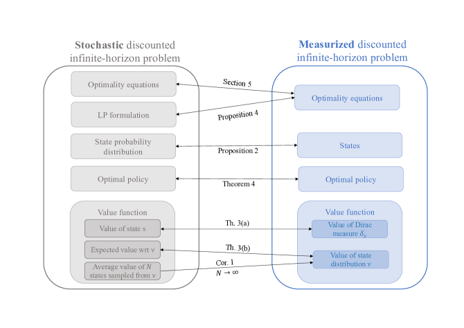
Figure 1: Outline of the theoretical results for the discounted infinite-horizon problem. This framework will be explored in Section 4.

All the theoretical results illustrated in Figure 1 express if-and-only-if relationships, except for the asymptotic result.

1.2 Structure of the paper

The remainder of the paper is structured as follows. We first briefly introduce the notation employed throughout the paper. Section 2 serves to lay out the notation and theory of classical stochastic MDPs. To make the paper self-contained we borrow the definitions and results from Hernández-Lerma and Lasserre (1996), to whom we are greatly indebted. Specifically, Sections 2.1 and 2.2 introduce the discounted infinite-horizon MDPs and its linear programming formulation, respectively. The reader is referred to Hernández-Lerma and Lasserre (1996) for more details on MDPs in general Borel state and action spaces, and to Puterman (2014) for a comprehensive review of MDPs in countable state and action spaces.

Section 3 formally defines measurized MDPs, and provides examples of augmented constraints and value function approximations. Section 4 mathematically establishes the connection between the lifted and original MDPs. More specifically, Sections 4.1, 4.2 and 4.3 show the relationship between stochastic and measurized states, value functions and policies, respectively. Section 5 demonstrates how to measurize a stochastic process and Section 6 shows the equivalence between the measurized MDP and the dual of the linear programming formulation. The last section is devoted to concluding remarks and future research avenues.

1.3 Notation

To make it easier to follow, we briefly introduce the notation used throughout this paper. We will use bold typeface to denote vectors and calligraphic font for sets and spaces.

Notation	Definition
$\mathcal{A}^{c}$	complementary of $\mathcal{A}$
$\mathcal{B}(\mathcal{S})$	Borel $\sigma$-algebra of $\mathcal{S}$
$\mathcal{M}(\mathcal{S})$	space of measures defined over a sample space $\mathcal{S}$
$\mathcal{M}_{+}(\mathcal{S})$	space of positive measures defined over a sample space $\mathcal{S}$
$\mathcal{M}_{\mathbb{P}}(\mathcal{S})$	space of probability measures defined over a sample space $\mathcal{S}$
$\mathcal{K}(\mathcal{U}|\mathcal{S})$	space of stochastic kernels defined over $\mathcal{U}$ given $\mathcal{S}$
$\mathbb{P}_{\nu}(\cdot)$	probability law induced by $\nu$
$\mathbb{E}_{\nu}[\cdot]$	expectation operator taken with respect to measure $\nu$
a.s.	almost surely

Table 1: Notation of sets, spaces, operators and abbreviations.

We also introduce the notation used for the different MDPs. We will use an overline to represent objects on the lifted space of measures, although measures themselves will be represented by Greek letters.

	Standard MDP	Measurized MDP
Abbreviation	MDP	$\mathcal{M}$-MDP
State space	$\mathcal{S}$	$\mathcal{M}_{\mathbb{P}}(\mathcal{S})$
States	$s$	$\nu$
Action space	$\mathcal{U}$	$\Phi$
Feasible action set	$\mathcal{U}(s)$	$\Phi(\nu)$
Actions	$u$	$\varphi$
Feasible set of state-action pairs	$\mathbb{K}$	$\overline{\mathbb{K}}$
Markovian decision rules	$\varphi(u|s)$	$\psi(\varphi|\nu)$
Markovian policies	$\pi=\{\varphi_{t}\}_{t\geq 0}$	$\overline{\pi}=\{\psi_{t}\}_{t\geq 0}$
Reward function	$r(s,u)$	$\overline{r}(\nu,\varphi)$
Transition kernel	$Q(\mathcal{A}|s,u),\ \mathcal{A}\in\mathcal{B}(\mathcal{S})$	$\overline{Q}(\mathcal{P}|\nu,\varphi),\ \mathcal{P}\in\mathcal{B}(\mathcal{M}_{\mathbb{P}}(\mathcal{S}))$
Optimal value function	$V^{*}(s)$	$\overline{V}^{*}(\nu)$

Table 2: Notation for the standard and measurized MDPs.

2 Standard stochastic MDPs

This section often quotes and summarizes definitions and theoretical results in Hernández-Lerma and Lasserre (1996). Additional definitions and results coming from this resource can be found in Appendix A. Following the notation in Table 2, we formally define Markov Decision Processes as follows.

Definition 1 (Hernández-Lerma and Lasserre (1996), Definition 2.2.1)

A Markov Decision Model is a five-tuple

$$(\mathcal{S},\mathcal{U},\{\mathcal{U}(s)|\ s\in\mathcal{S}\},Q,r)$$ (2)

consisting of

• a Borel space $\mathcal{S}$, called the state space and whose elements are referred to as states

• a Borel space $\mathcal{U}$, called the control or action set

• a family $\{\mathcal{U}(s)|\ s\in\mathcal{S}\}$ of nonempty measurable subsets $\mathcal{U}(s)$ of $\mathcal{U}$, where $\mathcal{U}(s)$ denotes the set of feasible actions when the system is in state $s$, and with the property that the set

  $$\mathbb{K}=\{(s,u)|\ s\in\mathcal{S},\ u\in\mathcal{U}(s)\}$$

  of feasible state-action pairs is a measurable subset of $\mathcal{S}\times\mathcal{U}$

• a stochastic kernel $Q$ on $\mathcal{S}$ given $\mathbb{K}$ called the transition law

• a measurable function $r:\ \mathbb{K}\rightarrow\mathbb{R}$ called the reward-per-stage function
  

Now assume that, at each period $t$, we observe the history $h_{t}=(s_{0},u_{0},...,s_{t-1},u_{t-1},s_{t})$ of the Markov Decision Model, with $(s_{k},u_{k})\in\mathbb{K}$ for all $k=0,...,t-1$ and $s_{t}\in\mathcal{S}$. We denote the set of all admissible histories as $\mathcal{H}_{t}=\mathbb{K}^{t}\times\mathcal{S}$. Then we define a randomized policy as follows.

Definition 2 (Hernández-Lerma and Lasserre (1996), Definition 2.2.3)

A randomized control policy is a sequence $\pi=\{\pi_{t}\}_{t=0,1,...}$ of stochastic kernels on the action set $\mathcal{U}$ given the set of all admissible histories $\mathcal{H}_{t}$, satisfying

$$\pi_{t}(\mathcal{U}(s_{t})|h_{t})=1\qquad\forall h_{t}\in\mathcal{H}_{t},\ t=0,1,...$$

The set of all randomized policies is denoted by $\Pi$.

Under certain conditions, the optimal policy may depend solely on the current state of the Markov process. In addition, we may sometimes find deterministic policies yielding the same expected reward as randomized policies. The following definition introduces these concepts.

Definition 3 (Hernández-Lerma and Lasserre (1996), Definitions 2.3.1 and 2.3.2)

Let $\Phi$ be the set of all Markovian stochastic kernels $\varphi$ on $\mathcal{U}$ given $\mathcal{S}$ such that $\varphi(\mathcal{U}(s)|s)=1$ for all $s\in\mathcal{S}$; i.e.

$$\Phi:=\{\varphi\in\mathcal{K}(\mathcal{U}|\mathcal{S}):\ \varphi(\mathcal{U}(s)|s)=1\quad\forall s\in\mathcal{S}\}.$$ (3)

Then a randomized Markov policy is a sequence $\pi=\{\varphi_{t}\}_{t\geq 0}$ where $\varphi_{t}\in\Phi$ for all $t\geq 0$. The set of all Markov randomized policies is denoted by $\Pi^{MR}$.

Let $\mathbb{F}$ be the set of all measurable functions $f:\mathcal{S}\rightarrow\mathcal{U}$ verifying $f(s)\in\mathcal{U}(s)$ for all $s\in\mathcal{S}$. Any function $f$ in $\mathbb{F}$ is called a selector. A policy $\pi=\{\varphi_{t}\}_{t\geq 0}$ such that $\varphi_{t}\in\Phi$ and there exists a $f_{t}\in\mathbb{F}$ satisfying $\varphi_{t}(f_{t}(s)|s)=1$ for all $t\geq 0$ is called a deterministic Markov policy. The set of all Markov deterministic policies is denoted by $\Pi^{MD}$. Moreover, if $f_{t}(\cdot)=f(\cdot)$ for all $t\geq 0$, then $\pi$ is called a deterministic stationary policy and we use the notation $\pi\in\Pi^{D}$.

By definition, we have that $\Pi^{D}\subset\Pi^{MD}\subset\Pi^{MR}\subset\Pi$. Now we use the definition of a control policy to lay out the unique probability distribution in the space of admissible histories according to Ionescu-Tulcea Theorem (see Proposition C.10 of Hernández-Lerma and Lasserre (1996)). This allows us to properly introduce discrete-time Markov Decision Processes.

Definition 4 (Hernández-Lerma and Lasserre (1996), Definition 2.2.4)

Let $(\Omega,\mathcal{F})$ be the measurable space consisting of the sample space $\Omega=(\mathcal{S}\times\mathcal{U})^{\infty}$ and $\mathcal{F}$ the corresponding product $\sigma$-algebra. Let $\pi=\{\pi_{t}\}_{t\geq 0}$ be an arbitrary control policy and $\nu_{0}$ the initial distribution on $\mathcal{S}$. Denote by $P_{\nu_{0}}^{\pi}$ the unique probability measure supported on $\mathcal{H}_{\infty}$ (see Ionescu-Tulcea Theorem), verifying

1. $P_{\nu_{0}}^{\pi}(s_{0}\in\mathcal{A})=\nu_{0}(\mathcal{A})\qquad\forall\mathcal{A}\in\mathcal{B}(\mathcal{S})$

2. $P_{\nu_{0}}^{\pi}(u_{t}\in\mathcal{C}|h_{t})=\pi_{t}(\mathcal{C}|h_{t})\qquad\forall\mathcal{C}\in\mathcal{B}(\mathcal{U}),t>0$

3. $P_{\nu_{0}}^{\pi}(s_{t}\in\mathcal{A}|h_{t},u_{t})=Q(\mathcal{A}|s_{t},u_{t})\qquad\forall\mathcal{A}\in\mathcal{B}(\mathcal{S}),\ t>0$.

Then the stochastic process $(\Omega,\mathcal{F},P_{\nu_{0}}^{\pi},\{s_{t}\}_{t\geq 0})$ is called a discrete-time Markov Decision Process.

2.1 Infinite-Horizon Discounted-Reward Problem

The following definition introduces $\alpha$-discount optimal policies, which maximize the discounted expected revenue along an infinite horizon.

Definition 5

We define the value function under policy $\pi\in\Pi$ as the infinite-horizon discounted reward

$$V(\pi,s_{0}):=\ \mathbb{E}_{s}^{\pi}\left[\sum_{t=0}^{\infty}\alpha^{t}r(s_{t},u_{t})\right]\qquad\forall s_{0}\in\mathcal{S},$$

where $\mathbb{E}_{s}^{\pi}$ is the expectation taken with respect to the probability $P^{\pi}_{\nu_{0}}$, being $\nu_{0}$ concentrated at $s$. We say $\pi^{*}\in\Pi$ is an $\alpha$-discount optimal policy, with $\alpha\in[0,1)$, if it verifies

$$V(\pi^{*},s_{0}):=\sup_{\Pi}\ V(\pi,s_{0}):=\sup_{\Pi}\ \mathbb{E}_{s}^{\pi}\left[\sum_{t=0}^{\infty}\alpha^{t}r(s_{t},u_{t})\right]\qquad\forall s_{0}\in\mathcal{S}.$$ (4)

We denote the optimal value function as $V^{*}(s_{0}):=V(\pi^{*},s_{0})$.

If the expectation in (4) is well defined, then $V(\cdot)$ is bounded for each $s\in\mathcal{S}$. Therefore, from now on we restrict ourselves to the space $\mathcal{V}(\mathcal{S})$ of bounded measurable functions in $\mathcal{S}$. In general, we assume that the state $s_{t}\in\mathcal{S}$ is observed and then an action $u_{t}\in\mathcal{U}(s_{t})$ is chosen. After this control is implemented, the probability that the MDP transitions to a state $s_{t+1}$ in the set $\mathcal{A}\in\mathcal{B}(\mathcal{S})$ is given by $Q(\mathcal{A}|s_{t},u_{t})$.

Hernández-Lerma and Lasserre (1996) also provides a more generalized formulation for (4) when the probability distribution $\nu_{0}$ of the initial state $s_{0}$ is given, i.e.

$$\mathbb{V}^{*}(\nu_{0}):=\sup_{\Pi}\ \int_{\mathcal{S}}V(\pi,s)d\nu_{0}=\sup_{\Pi}\ \mathbb{E}_{\nu_{0}}^{\pi}\left[\sum_{t=0}^{\infty}\alpha^{t}r(s_{t},u_{t})\right]\qquad\forall\nu_{0}\in\mathcal{M}_{\mathbb{P}}(\mathcal{S}).$$ (5)

The definition of $\mathbb{V}^{*}(\cdot)$ is related to our measurized value function, as it evaluates state distributions rather than stochastic states themselves. Section 4.2 outlines the relationship between $\mathbb{V}^{*}(\cdot)$ and $\overline{V}^{*}(\cdot)$.

We now introduce some necessary assumptions for the existence of an optimal deterministic stationary policy (Hernández-Lerma and Lasserre, 1996, Chapter 4).

Assumption 2.1 (Hernández-Lerma and Lasserre (1996), Assumption 4.2.1)

aaa

1. The one-stage reward $r$ is upper semicontinuous, upper bounded, and sup-compact in $\mathbb{K}$

2. Q is either

   • weakly continuous

   • strongly continuous

Assumption 2.2 (Hernández-Lerma and Lasserre (1996), Assumption 4.2.2)

There exists a policy $\pi$ such that $V(\pi,s)<\infty$ for each $s\in\mathcal{S}$.

For definitions of upper semicontinuous functions, and strongly and weakly continuous kernels, the reader is referred to Appendix A. The only difference of working in the weakly case instead of in strongly continuous case is that the value function belongs to the set of upper semicontinuous rather than just measurable functions (see Theorem 3.3.5 in Hernández-Lerma and Lasserre (1996)). In this paper, we adopt Assumptions 2.1(a),(b2) and 2.2 for the original MDP. Proposition 1 will show that then the lifted MDP inherits Assumptions 2.1(a),(b1) and 2.2. The transition kernel of the measurized MDP is not strongly continuous because the transition is deterministic in the lifted space of probability measures (i.e., the measurized kernel is a Dirac measure). More details can be seen in the proof of Proposition 1, that can be found in Appendix B.

The following theorem shows that if Assumptions 2.1 and 2.2 hold, we can restrict ourselves to the set $\Pi^{D}$ of deterministic stationary policies without loss of optimality, and reformulate the infinite horizon problem (4) using the optimality equations ($\alpha$-DCOE).

Theorem 1 (Hernández-Lerma and Lasserre (1996), Theorem 4.2.3)

Suppose Assumptions 2.1 and 2.2 hold. Then

• The $\alpha$-discount value function $V^{*}(\cdot)$ is the pointwise maximal solution to ($\alpha$-DCOE) , and if $V(\cdot)$ is another solution to ($\alpha$-DCOE), then $V(\cdot)\leq V^{*}(\cdot)$.

• There exists a selector $f^{*}\in\mathbb{F}$ such that $f^{*}(s)\in\mathcal{U}(s)$ attains the maximum in ($\alpha$-DCOE); i.e., the deterministic stationary policy $f_{\infty}^{*}=\{f^{*}\}_{t\geq 0}$ is $\alpha$-discount optimal; conversely, if $f_{\infty}^{*}\in\Pi^{DS}$ is $\alpha$-discount optimal, then it solves ($\alpha$-DCOE).

• If $\lim_{t\to\infty}\alpha^{t}\mathbb{E}_{s}^{\pi}\left[V(\pi^{*},s_{t})\right]=0$ for all $\pi\in\Pi^{0}$ and $s\in\mathcal{S}$, then $\pi^{*}$ is $\alpha$-discount optimal if and only if $V(\pi^{*},\cdot)$ satisfies ($\alpha$-DCOE).

• If an $\alpha$-discount optimal policy exists, then there exists one that is deterministic stationary.

That is to say, the previous theorem shows that under certain assumptions the deterministic stationary policy $\pi^{*}=\{\varphi_{t}^{*}\}_{t\geq 0}$, with $\varphi^{*}_{t}(f^{*}(s)|s)=1$ for all $t=0,1,...$, is an $\alpha$-discount optimal solution to the traditional MDP (4). For what follows we frame our distributional approach to MDPs from Markovian stochastic kernels; i.e., we replace $\Pi$ by $\Pi^{MR}$ in (5). Moreover, Theorem 1 and Lemma 4.2.7 in Hernández-Lerma and Lasserre (1996) entail that $V^{*}\in\mathcal{V}(\mathcal{S})$ is the unique bounded solution to ($\alpha$-DCOE) for a bounded reward function $r$ (see Note 4.2.1 in Hernández-Lerma and Lasserre (1996) for more details on this).

Finally, throughout the paper we adopt Assumptions 2.1 and 2.2; we detail in proofs when they are necessary. In addition, we will also make the following assumption so the Monotone Convergence Theorem can be applied.

Assumption 2.3

The reward function $r$ is bounded below.

Given Assumption 2.1 and the newly introduced requirement, it follows, without loss of generality, that the reward function can be taken to be non-negative.

2.2 The linear programming formulation

In this section, we introduce the linear programming formulation of the optimality equations ($\alpha$-DCOE). The reader is referred to Chapter 6 in Hernández-Lerma and Lasserre (1996) for details on how to derive this LP and the theoretical results showing its equivalency with the ($\alpha$-DCOE). Let $\nu_{0}\in\mathcal{M}_{\mathbb{P}}(\mathcal{S})$ be any distribution over the states; then the following linear program retrieves the optimal value function $\nu_{0}$-almost surely

$$\inf_{V(\cdot)} \ \int_{\mathcal{S}}V(s)d\nu_{0}(s)$$ (LP)

s.t. $$\ V(s)\geq r(s,u)+\alpha\int_{\mathcal{S}}V(s^{\prime})Q(ds^{\prime}|s,u)\qquad\qquad\forall s\in\mathcal{S},\forall u\in\mathcal{U}(s).$$

Denote $\mathcal{U}(\mathcal{A})=\cup_{s\in\mathcal{A}}\mathcal{U}(s)$ as the set of feasible actions that can be taken from set $\mathcal{A}\in\mathcal{B}(\mathcal{S})$; then the dual of (LP) is

$$\sup_{\zeta\in\mathcal{M}_{+}(\mathbb{K})} \ \int_{\mathcal{S}}\int_{\mathcal{U}(\mathcal{S})}r(s,u)\ d\zeta(s,u)$$ (D_ζ)

s.t. $$\ \zeta(\mathcal{A},\mathcal{U}(\mathcal{A}))=\nu_{0}(\mathcal{A})+\alpha\int_{\mathcal{S}}\int_{\mathcal{U}(\mathcal{A})}Q(\mathcal{A}|s,u)d\zeta(s,u) \forall\mathcal{A}\in\mathcal{B}(\mathcal{S})$$

where measure $\zeta\in\mathcal{M}_{+}(\mathbb{K})$ is the dual variable associated with the constraints in (LP). This measure is defined on $\mathbb{K}$ because the constraints in the primal apply exclusively to feasible state-action pairs. Note that $\zeta$ is not a probability measure because $\zeta(\mathcal{S},\mathcal{U}(\mathcal{S}))=1/(1-\alpha)$ for the constraint with $\mathcal{A}=\mathcal{S}$. Indeed, $\zeta$ can be interpreted as an expected discounted state-action frequency. The next theorem summarizes some of the theoretical results in Hernández-Lerma and Lasserre (1996)

Theorem 2

Under Assumptions 2.1 and 2.2, the optimal solution $V^{*}(\cdot)$ to (LP) coincides with the optimal value function retrieved from optimality equations ($\alpha$-DCOE) $\nu_{0}$-almost surely. Moreover, (D_ζ) is solvable and strong duality holds: i.e.,

$$\int_{\mathcal{S}}V^{*}(s)d\nu_{0}(s)=\int_{\mathcal{S}}\int_{\mathcal{U}(\mathcal{S})}r(s,u)\ d\zeta^{*}(s,u),$$

where $\zeta^{*}$ is the optimal solutions to (D_ζ).

3 Measurized MDPs

In this section, we introduce the so-called measurized MDPs, denoted $\mathcal{M}$-MDPs. These are standard MDPs that have been lifted to the space of probability measures. The formal definition is as follows.

Definition 6

Let $(\mathcal{S},\mathcal{U},\{\mathcal{U}(s)|\ s\in\mathcal{S}\},Q,r)$ be a standard MDP. A measurized MDP $(\mathcal{M}_{\mathbb{P}}(\mathcal{S}),\Phi,\{\Phi(\nu)|\ \nu\in\mathcal{M}_{\mathbb{P}}(\mathcal{S})\},\overline{Q},\overline{r})$ is a measure-valued MDP such that:

• a state $\nu\in\mathcal{M}_{\mathbb{P}}(\mathcal{S})$ is a probability measure over the states $s\in\mathcal{S}$ of the standard MDP

• the action space $\Phi:=\{\varphi\in\mathcal{K}(\mathcal{U}|\mathcal{S}):\ \varphi(\mathcal{U}(s)|s)=1\ \forall s\in\mathcal{S}\}$ is the set of feasible Markovian decision rules of the standard MDP

• $\Phi(\nu)$ is the set of admissible actions from state $\nu$ such that $\Phi(\nu)\subseteq\Phi$

• the transition kernel $\overline{Q}$ is deterministic. More specifically, the next state of the measurized MDP is a measure computed according to a function $F:\mathcal{M}_{\mathbb{P}}(\mathcal{S})\times\mathcal{K}(\mathcal{U}|\mathcal{S})\rightarrow\mathcal{M}_{\mathbb{P}}(\mathcal{S})$, defined as

  $$\nu^{\prime}(\cdot)=F(\nu,\varphi)(\cdot):=\int_{\mathcal{S}}\int_{\mathcal{U}}Q(\cdot|s,u)\varphi(du|s)d\nu(s).$$ (6)

  Therefore, $\overline{Q}$ can be expressed using (6) as

  $$\overline{Q}(\mathcal{P}|\nu,\varphi)=\left\{\begin{array}[]{ll}1&\quad\mbox{ if F$(\nu,\varphi)\in\mathcal{P}$}\\ 0&\quad\mbox{ otherwise}\\ \end{array}\right.$$ (7)

• the reward function $\overline{r}$ is the expected revenue of the standard MDP computed with respect to a distribution $\nu\in\mathcal{M}_{\mathbb{P}}(\mathcal{S})$ and a stochastic kernel $\varphi\in\mathcal{K}(\mathcal{U}|\mathcal{S})$; i.e.,

  $$\overline{r}(\nu,\varphi):=\mathbb{E}_{\nu}\mathbb{E}_{\varphi}[r(s,u)]=\int_{\mathcal{S}}\int_{\mathcal{U}}r(s,u)\ \varphi(du|s)d\nu(s).\\$$ (8)

Later we will show conditions under which $\Phi(\nu)$ need not depend on $\nu$, without loss of optimality. In that case, where $\Phi(\nu)=\Phi$, we say that the MDP is the measurized counterpart of the original MDP. If, on the other hand, $\Phi(\nu)\subseteq\Phi$, we say that the lifted MDP is a tightened measurized MDP.

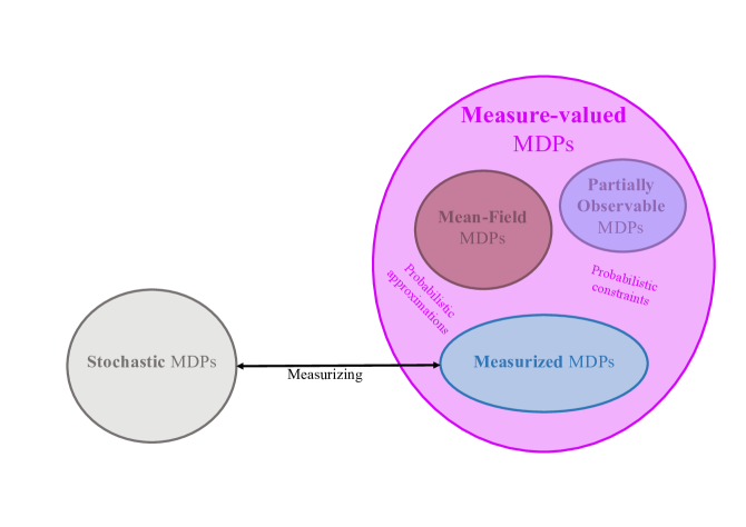
Figure 2: Illustration of the unifying measure-valued framework.

Measurized MDPs constitute a specific category within the broader class of measure-valued MDPs, where states themselves are treated as measures. For further information on measure-valued MDPs, including a formal definition and illustrative examples featuring POMDPs and MFMDPs within this framework, the reader is referred to Appendix C. Therefore, the measure-valued framework, depicted in Figure 2, serves as the overarching context to which measurized MDPs belong. Since measurized MDPs are a special class of MDPs, the optimal measurized value function can be defined as usual

$$\overline{V}^{*}(\nu_{0}):=\sup_{\overline{\pi}\in\overline{\Pi}}\ \mathbb{E}_{\nu_{0}}^{\overline{\pi}}\left[\sum_{t=0}^{\infty}\alpha^{t}\overline{r}(\nu,\varphi)\right],$$ (9)

where $\overline{\Pi}:=\{\psi_{t}\}_{t\geq 0}$ is the set of all Markovian decision rules for the measurized MDP. The following result shows that the lifting procedure preserves the assumptions adopted for the original MDP, albeit the transition kernel becomes weakly continuous.

Proposition 1

The measurized MDP $(\mathcal{M}_{\mathbb{P}}(\mathcal{S}),\Phi,\{\Phi(\nu)|\ \nu\in\mathcal{M}_{\mathbb{P}}(\mathcal{S})\},\overline{Q},\overline{r})$ follows Assumptions 2.1(a), (b1) and 2.2 if the original MDP follows the Assumptions 2.1(a), (b2) and 2.2 and the set of feasible actions $\Phi(\nu)$ is closed for every $\nu\in\mathcal{M}_{\mathbb{P}}(\mathcal{S}).$

The proof of this result is in Appendix B.. Therefore, Theorem 1 applies and we can restrict ourselves to the set of deterministic stationary decision rules. That is to say, the supremum in the infinite-horizon problem above is attainable and there exists a selector $\overline{f}^{*}:\mathcal{M}_{\mathbb{P}}(\mathcal{S})\to\Phi$ such that $\overline{f}^{*}(\nu)\in\Phi(\nu)$ for all $\nu\in\mathcal{M}_{\mathbb{P}}(\mathcal{S})$ and $\overline{f}^{*}$ is the solution to (9). In other words, we can optimize over the set $\overline{\Pi}^{D}:=\{\psi_{t}\in\overline{\Pi}:\ \psi_{t}=\psi\ \forall t\geq 0\mbox{ and }\forall\nu\in\mathcal{M}(\mathcal{S}),\ \exists\varphi\in\Phi(\nu)\mbox{ s.t. }\psi(\varphi|\nu)=1\}$. Since the transition to the next state is deterministic and the Monotone Convergence Theorem allows us to interchange the expectation and the infinite sum, we get that

$$\overline{V}^{*}(\nu_{0})=\sup_{\begin{subarray}{c}\varphi_{t}\in\Phi(\nu_{t})\\ \forall t\geq 0\end{subarray}}\left\{\sum_{t=0}^{\infty}\alpha^{t}\overline{r}(\nu_{t},\varphi_{t})\right\},$$ (10)

where $\nu_{t}=F(\nu_{t-1},\varphi_{t-1})$ for all $t\geq 1$. Finally, Theorem 1 ensures that one can retrieve the optimal measurized value function $\overline{V}^{*}(\cdot)$ and the optimal measurized actions $\overline{f}^{*}(\nu)$ from

$$\overline{V}^{*}(\nu) =\sup_{\varphi\in\Phi(\nu)}\ \left\{\overline{r}(\nu,\varphi)+\alpha\overline{V}^{*}(F(\nu,\varphi))\right\}\qquad\forall\nu\in\mathcal{M}_{\mathbb{P}}(\mathcal{S}). \mathcal{M} \alpha$$ (--DCOE)

Bäuerle (2023) obtained similar deterministic equations for MFMDPs without common noise. More details on Bäuerle (2023) and how it relates to the measurized MDPs can be found in Appendix D. Since the measurized MDP inherits Assumption 2.1 and 2.2 from its original MDP, Theorem 2 also applies, yielding the following linear programming formulation that is essentially equivalent to ($\mathcal{M}$-$\alpha$-DCOE)

$$\inf_{\overline{V}(\cdot)} \ \overline{V}(\nu_{0}) \mathcal{M}$$ (-LP)

s.t. $$\ \overline{V}(\nu)\geq\overline{r}(\nu,\varphi)+\alpha\overline{V}(F(\nu,\varphi))\qquad\qquad\forall\nu\in\mathcal{M}_{\mathbb{P}}(\mathcal{S}),\forall\varphi\in\Phi(\nu).$$

One can think of the measurized MDP as aiming to optimize the distribution of the states through controls that are stochastic kernels over the original actions $u$. For any initial state distribution $\nu_{0}$ and any measurized policy $\overline{\pi}=\{\varphi_{t}\}_{t\geq 0}$ the trajectory of state distributions $\{F(\nu_{t},\varphi_{t})\}_{t\geq 1}$ can be computed deterministically using (6), thus giving rise to a deterministic process. In particular, an optimal policy $\overline{\pi}^{*}:=\{\varphi_{t}^{*}\}_{t\geq 0}$ to the measurized MDP gives rise to an optimal trajectory of state distributions

$$\Upsilon^{*}:=\{\nu_{t}^{*}\}_{t\geq 0},$$ (11)

where $\nu_{t}^{*}:=F(\nu_{t-1}^{*},\varphi_{t-1}^{*})$ for $t\geq 1$. In addition, the measurized framework facilitates the understanding of which actions we expect to take most frequently under a certain distribution of the states. More specifically, if at period $t$ the states are distributed according to $\nu_{t}$, we can define the distribution of actions under decision rule $\varphi_{t}$ as

$$\rho_{t}(\mathcal{D}):=\int_{\mathcal{S}}\varphi_{t}(\mathcal{D}|s)d\nu_{t}(s).\qquad\forall\mathcal{D}\in\mathcal{B}(\mathcal{U}).$$ (12)

In Section 6 we will show that $\rho_{t}$ is well defined, since for every pair $\varphi_{t},\ \nu_{t}$ there exists a unique $\rho_{t}$ and vice-versa.

3.1 Probabilistic constraints

Interestingly, the set of admissible actions $\Phi(\nu)$ is contingent on the current state distribution $\nu$. This enables the modelling of probabilistic constraints on the states of the original MDP. For instance, one can set constraints on various risk measures related to the agent’s future perceived costs or limit moments of future distributions over original states. Furthermore, one could also impose restrictions on the distribution of actions taken in the original MDP. These constraints do not arise naturally outside the measurized framework.

The following example illustrates how one could easily introduce Conditional Value at Risk (CVaR) constraints in the measurized framework. Handling such risk constraints is notably challenging in the conventional framework, leading much of the literature to focus on finite horizon MDPs and bounding the CVaR of discounted accumulated costs at a terminal stage, as seen in works like Borkar and Jain (2014). A more recent work Xia and Glynn (2022) considers a long-run average MDP with finite state and action spaces, and optimizes the CVaR at the steady state. As the authors mention “dynamically optimizing CVaR is difficult since it is not a standard Markov decision process (MDP) and the principle of dynamic programming fails”. In contrast, we offer here a more straightforward alternative within our framework.

Example 3.1 (MDPs with CVaR constraints )

Consider a standard MDP with cost function $c:\mathcal{S}\times\mathcal{U}\rightarrow\mathbb{R}$. The optimality equations of its measurized counterpart with no additional constraints are

$$\overline{V}^{*}(\nu) =\inf_{\varphi\in\Phi}\ \left\{\int_{\mathcal{S}}\int_{\mathcal{U}}c(s,u)\varphi(du|s)d\nu(s)+\alpha\overline{V}^{*}(F(\nu,\varphi))\right\},\qquad\forall\nu\in\mathcal{M}_{\mathbb{P}}(\mathcal{S}).$$

Here $\nu$ is the distribution of states of the original MDP, to which we want to add a CVaR constraint, and $\nu^{\prime}(\cdot)=F(\nu,\varphi)(\cdot)$ is the subsequent state distribution. Define the Value at Risk (VaR_β) at the current period as

$$VaR_{\beta}(c;\nu,\varphi):=\arg\inf_{a\in\mathbb{R}}\left\{\mathbb{P}_{\nu,\varphi}(c(s,u)\leq a)\geq\beta\right\}.$$

This measure quantifies the potential financial loss or risk within a specified confidence level $\beta>0$.

We now explore how to write and interpret the Value at Risk within an MDP. For simplicity, consider $\mathcal{S}\subseteq\mathbb{R}$ and $\mathcal{U}\subseteq\mathbb{R}$. For every $s\in\mathcal{S}$, $a\in\mathbb{R}$, denote $\mathcal{U}_{s,a}:=\{u\in\mathcal{U}(s):c(s,u)\leq a\}$. Given $\nu$ and $\varphi$, we can express $VaR_{\beta}$ as

$$VaR_{\beta}(c;\nu,\varphi) =\arg\inf_{a\in\mathbb{R}}\left\{\mathbb{P}_{\nu,\varphi}(c(s,u)\leq a)\geq\beta\right\}$$

$$=\arg\inf_{a\in\mathbb{R}}\left\{\int_{s\in\mathcal{S}}\int_{u\in\mathcal{U}_{s,}}\varphi(du|s)d\nu(s)\geq\beta\right\}$$

$$=\arg\inf_{a\in\mathbb{R}}\left\{\int_{s\in\mathcal{S}}\varphi(\mathcal{U}_{s,a}|s)d\nu(s)\geq\beta\right\},$$

$$=\arg\inf_{a\in\mathbb{R}}\left\{\rho(\mathcal{U}_{s,a})\geq\beta\right\},$$

where $\rho$ is the distribution of actions (12), which depends on $\nu$ and $\varphi$. If we think of the set $\mathcal{U}_{s,a}$ as the set of “safe actions” to take from state $s$, we can see the $VaR_{\beta}$ as the minimum value $a^{*}$ such that the actions taken “are safe” with a probability larger or equal to $\beta$. Increasing $\beta$ amounts to expanding that set so that the decisions taken are “more often” therein. In other words, the larger the $\beta$, the larger the set of actions we consider as “safe”.

We now focus on the conditional VaR, which we define using the Acerbi’s formula, to which we plug the VaR computed with respect to probability $\mathbb{P}_{\nu,\varphi}$

$$CVaR_{\upsilon}(c) :=\frac{1}{1-\upsilon}\int_{\upsilon}^{1}VaR_{\beta}(c)d\beta$$ (13)

$$=\frac{1}{1-\upsilon}\int_{\upsilon}^{1}\arg\inf_{a\in\mathbb{R}}\left\{\rho(\mathcal{U}_{s,a})\geq\beta\right\}d\beta,$$

In the equation above, threshold $\beta\in(0,1)$ is not given. Instead, we integrate with respect to $\beta$ for a “reasonable” interval of values (e.g. if $\upsilon=0.95$ we consider $\beta\in[0.95,1)$). This provides an “average VaR”, i.e., the expected threshold $a^{*}$ such that the actions taken “are safe” within a reasonable range of probabilities.

Assume now that we want to bound the CVaR so it does not exceed a threshold $\theta>0$ at any decision period of the MDP. Integrating this requirement into the optimality equations yields the CVaR-constrained MDP

$$\overline{V}^{*}(\nu)=\inf_{\varphi\in\Phi} \ \left\{\int_{\mathcal{S}}\int_{\mathcal{U}}c(s,u)\varphi(du|s)d\nu(s)+\alpha\overline{V}^{*}(F(\nu,\varphi))\right\},\hskip 71.13188pt\forall\nu\in\mathcal{M}_{\mathbb{P}}(\mathcal{S})$$

s.t. $$\ \frac{1}{1-\upsilon}\int_{\upsilon}^{1}\arg\inf_{a\in\mathbb{R}}\left\{\rho(\mathcal{U}_{s,a})\geq\beta\right\}d\beta\leq\theta$$

aaaa $\blacksquare$

3.2 Value function approximations

In the usual MDP framework, value function approximations are often modelled as the weighted sum of basis functions $\phi_{k}:\mathcal{S}\to\mathbb{R}$, yielding

$$V(s)\approx\sum_{k=1}^{K}w_{k}\phi_{k}(s).$$ (14)

Some choices for $\phi_{k}(\cdot)$ that have been explored in the literature are linear Adelman (2007), separable piecewise linear Vossen and Zhang (2015) or ridge exponential Adelman et al. (2023). The theoretical results developed in the following section (and, more specifically, Theorem 3.(b)) ensures that imposing an approximation (14) in the original MDP translates into an approximation in expected value; i.e.,

$$\overline{V}(\nu)\approx\sum_{k=1}^{K}\overline{w}_{k}\mathbb{E}_{\nu}[\phi_{k}(s)].$$ (15)

Interestingly, considering a measurized MDP whose states are probability measures in state-space $\mathcal{S}$ allows one to model a broader class of basis functions that are contingent on $\nu$, yielding

$$\overline{V}(\nu)\approx\sum_{k=1}^{K}\overline{w}_{k}\overline{\phi}_{k}(\nu).$$ (16)

Certain basis functions $\overline{\phi}_{k}(\cdot)$ may not be accessible within the original framework. To illustrate this, the subsequent example introduces some compelling measure-valued approximations.

Example 3.2 (Some augmented basis functions)

There are multiple measurized basis functions $\overline{\phi}$ that can be written as the expected value of some original basis function $\phi$. For instance, if $a>0$ is a scalar and the state space is one-dimensional, the following measurized basis functions can be considered in the augmented space:

• Basis functions like $\overline{\phi}_{k}(\nu)=\int_{\mathcal{S}}s^{a}d\nu(s)=\mathbb{E}_{\nu}[s^{a}]$ provide a moment approximation, generated by $\phi_{k}(s)=s^{a}$.

• One could consider Laplace transforms as basis functions; i.e., $\overline{\phi}_{k}(\nu)=\int_{\mathcal{S}}e^{as}d\nu(s)=\mathbb{E}_{\nu}[e^{as}]$, generated by $\phi_{k}(s)=e^{as}$.

• In addition, basis functions could be chosen as generating functions of the state $s$, having $\overline{\phi}_{k}(\nu)=\int_{\mathcal{S}}a^{s}d\nu(s)=\mathbb{E}_{\nu}[a^{s}]$, when $\phi_{k}(s)=a^{s}$.

• Furthermore, consider a state $s$ taking values in $\mathbb{R}$. For instance, $s$ might measure the risk of cardiovascular disease in a patient, the losses incurred by a portfolio… etc. One could include probabilistic basis functions like $\overline{\phi}_{k}(\nu)=\mathbb{P}_{\nu}(s>a)$, with $a\in[0,100]$, to approximate the value of the current risk distribution $\overline{V}^{*}(\nu)$. Here $\phi_{k}(s)=\mathbf{1}_{\{s>a\}}$, where $\mathbf{1}_{\{\cdot\}}$ is the indicator function.

However, many other basis functions in the lifted space are different in nature, in the sense that they cannot be written merely as expected values of some function $\phi_{k}(s)$ of the random state $s$. For example:

• One could use the Conditional Value at Risk (13) as a basis function. Diverse basis functions arise for different values of the threshold $\beta$.

• Basis functions could measure the distance to a benchmark distribution $\mu$; for instance:

  • $\overline{\phi}(\nu)$ can be the Wasserstein $p$-distance between $\nu$ and $\mu$

    $$\overline{\phi}(\nu)=\left(\inf_{\gamma\in\Gamma(\nu,\mu)}\int_{\mathcal{S}}\|s-x\|_{p}d\gamma(s,x)\right)^{1/p}$$

    where $p\geq 1$ and $\Gamma(\nu,\mu)$ is the set of all joint distributions $\gamma$ in $\mathcal{S}\times\mathcal{S}$ with marginals $\nu$ and $\mu$. Note that different values of $p$ yield different basis functions.

  • Instead, one could consider the Kullback–Leibler divergence as a basis function

    $$\overline{\phi}(\nu)=\int_{\mathcal{S}}log\left(\frac{d\nu}{d\mu}\right)d\nu(s),$$

    where $d\nu/d\mu$ is the Radon-Nikodym derivative of $\nu$ with respect to $\mu$.

Note that (a)-(d) are available in the standard Approximate Dynamic Programming context, because they derive from standard basis functions. They become moment approximations in the measurized framework but do not provide any additional approximation power. In contrast, (e)-(f) could not have been handled until now. aa $\blacksquare$

4 Connection between measurized and stochastic MDPs

This section is devoted to analyzing the connection between the original MDP and its measurized counterpart; i.e., the lifted MDP with $\Phi(\nu)=\Phi$ for all $\nu\in\mathcal{M}_{\mathbb{P}}(\mathcal{S})$. In particular, we relate the states of the $\mathcal{M}$-MDP to the probability distribution $P_{\nu_{0}}^{\pi}$ of Ionescu-Tulcea Theorem, introduced in Definition 4. Moreover, we show that, although the measurized value function evaluates probability distributions in $\mathcal{M}_{\mathbb{P}}(\mathcal{S})$, the original value function can be retrieved when plugging Dirac measures concentrated at the current state. Finally, we show that these two formulations share optimal solutions, which according to Theorem 1, belong to $\Pi^{D}$.

4.1 Relationship between states

In this section, we show the relationship between the measurized and original states, summarized in Figure 3.

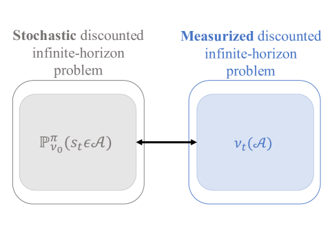
Figure 3: Equivalence between the states $\nu$ of measurized MDP and the states $s$ of the original MDP it was lifted from.

Let $\pi=\{\varphi_{t}\}_{t\geq 0}$; Theorem 1 enables one to consider exclusively either deterministic or randomized Markovian policies without loss of optimality. Then using the definition of the revenue function (8), we can rewrite the infinite horizon problem (5) as the discounted measurized MDP problem as follows

$$\mathbb{V}^{*}(\nu_{0}) =\sup_{\pi\in\Pi^{MR}}\mathbb{E}_{\nu_{0}}^{\pi}\left[\sum_{t=0}^{\infty}\alpha^{t}r(s_{t},u_{t})\right] \nu_{0}\in\mathcal{M}(\mathcal{S})$$

$$=\sup_{\begin{subarray}{c}\varphi_{t}\in\Phi,\\ t\geq 0\end{subarray}}\ \sum_{t=0}^{\infty}\alpha^{t}\mathbb{E}_{\nu_{t}}\mathbb{E}_{\varphi_{t}}[r(s,u)] \nu_{0}\in\mathcal{M}(\mathcal{S})$$ (17)

$$=\sup_{\begin{subarray}{c}\varphi_{t}\in\Phi,\\ t\geq 0\end{subarray}}\ \sum_{t=0}^{\infty}\alpha^{t}\overline{r}(\nu_{t},\varphi_{t}) \nu_{0}\in\mathcal{M}(\mathcal{S})$$

$$=\overline{V}^{*}(\nu_{0})$$

where the second equality arises from the Monotone Convergence Theorem (which needs Assumptions 2.1 and 2.3) and the last equality comes from (10). This proves that the optimal solution $\mathbb{V}^{*}(\cdot)$ to (5) coincides with the optimal measurized value function $\overline{V}^{*}(\cdot)$ at every state distribution $\nu\in\mathcal{M}(\mathcal{S})$. Through (17), one can intuit a connection between the distributions $\nu_{t}$ controlled through $\varphi_{t}$ and the probability distribution $P_{\nu_{0}}^{\pi}$. We explicitly state this relationship in the following proposition.

Proposition 2

Define the policy $\pi=\{\varphi_{t}\}_{t\geq 0}$. Then the sample path $\Upsilon=\{\nu_{t}\}_{t\geq 0}$, with $\nu_{t+1}=F(\nu_{t},\varphi_{t})$ for all $t\geq 0$, is related to the probability distribution $P_{\nu_{0}}^{\pi}$ as follows

$$P_{\nu_{0}}^{\pi}(s_{t+1}\in\mathcal{A})=\nu_{t+1}(\mathcal{A})\qquad\forall\mathcal{A}\in\mathcal{B}(\mathcal{S})$$ (18)

Proof.

For this proof we adopt Assumptions 2.1 and 2.2. According to Remark C.11 in Hernández-Lerma and Lasserre (1996), the probability measure $P_{\nu_{0}}^{\pi}$ has the following expression for all $t\geq 0$

$$P_{\nu_{0}}^{\pi}(s_{t+1}\in\mathcal{A}_{t+1}) =\medmath$$

We prove this proposition by induction

$\bullet$Prove for t=0:  $P_{\nu_{0}}^{\pi}(s_{0}\in\mathcal{A}_{0})=\int_{\mathcal{A}_{0}}\nu_{0}(ds_{0})=\nu_{0}(\mathcal{A}_{0}).$

$\bullet$Prove for t=1:

$$P_{\nu_{0}}^{\pi}(s_{1}\in\mathcal{A}_{1}) =\int_{\mathcal{S}}\int_{\mathcal{U}}\int_{\mathcal{A}_{1}}Q(ds_{1}|s_{0},u_{0})\varphi_{0}(du_{0}|s_{0})\nu_{0}(ds_{0})$$

$$=\int_{\mathcal{S}}\int_{\mathcal{U}}Q(\mathcal{A}_{1}|s_{0},u_{0})\varphi_{0}(du_{0}|s_{0})\nu_{0}(ds_{0})$$

$$=F(\nu_{0},\varphi_{0})$$

$$=\nu_{1}(\mathcal{A}_{1})$$

where the last equality comes from (6).

$\bullet$Assume true for t:  $P_{\nu_{0}}^{\pi}(s_{t}\in\mathcal{A}_{t})=\nu_{t}(\mathcal{A}_{t}).$

$\bullet$Prove for t+1:

$$\nu_{t+1}(\mathcal{A}_{t+1}) =\int_{\mathcal{S}}\int_{\mathcal{U}}Q(\mathcal{A}_{t+1}|s_{t},u_{t})\varphi_{t}(du_{t}|s_{t})d\nu_{t}(s_{t})$$

$$=\int_{\mathcal{S}}\nu_{0}(ds_{0})\int_{\mathcal{U}}\int_{\mathcal{S}}Q(ds_{1}|s_{0},u_{0})\varphi_{0}(du_{0}|s_{0})\int_{\mathcal{U}}\int_{\mathcal{S}}Q(ds_{2}|s_{1},u_{1})\varphi_{1}(du_{1}|s_{1})\ldots\int_{\mathcal{U}}Q(\mathcal{A}_{t+1}|s_{t},u_{t})\varphi_{t}(du_{t}|s_{t})$$

$$=P_{\nu_{0}}^{\pi}(s_{t+1}\in\mathcal{A}_{t+1})$$

where the second equality comes from the fact that $\nu_{t}(\mathcal{A}_{t})=P_{\nu_{0}}^{\pi}(s_{t}\in\mathcal{A}_{t})$ and hence we can plug the expression of $P_{\nu_{0}}^{\pi}$ as defined in (4.1). $\square$

4.2 Relationship between optimal value functions

In this section, we provide various theoretical results that link the measurized value function $\overline{V}^{*}(\cdot)$ with the stochastic value function $V^{*}(\cdot)$ from the original MDP that was lifted. Figure 4 summarizes the results.

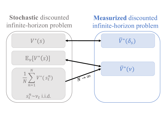
Figure 4: Connection between the original value function $V^{*}(\cdot)$ and the measurized value function $\overline{V}^{*}(\cdot)$. Bidirectional arrows show equivalence; the unidirectional arrow indicates an asymptotic result.

The following theorem shows that the stochastic and measurized value functions coincide if the latter is evaluated at a Dirac measure $\delta_{s}$ concentrated at the stochastic state $s$. In addition, it also shows that the supremum in (5) can be interchanged with the integral, hence yielding that the measurized value function is the expected stochastic value function.

Theorem 3

Let $V^{*}(\cdot)$ and $\overline{V}^{*}(\cdot)$ be the solutions to ($\alpha$-DCOE) and ($\mathcal{M}$-$\alpha$-DCOE), respectively. Then

$$(a) \qquad\overline{V}^{*}(\delta_{s})=V^{*}(s) \forall s\in\mathcal{S}$$

$$(b) \qquad\overline{V}^{*}(\nu)=\int_{\mathcal{S}}V^{*}(s)d\nu(s)=\mathbb{E}_{\nu}[V^{*}(s)] \nu\in\mathcal{M}_{\mathbb{P}}(\mathcal{S})$$

Proof.

In this proof we use Assumptions 2.1, 2.2, and 2.3.

We start by proving (a). Let $\nu_{0}=\delta_{s}$ and denote $\nu_{t}$ as the distribution of the states at time $t$, i.e. $s_{t}\sim\nu_{t}$. Proposition 2 showed that these distributions can be computed through the recursive equation $\nu_{t}=F(\nu_{t-1},\varphi_{t-1})$, for all $t=1,2,...$. According to Theorem 1, we can restrict ourselves to deterministic or randomized Markovian policies without loss of optimality. Then we can use Equation (4) to find an $\alpha$-discount optimal policy as

$$V^{*}(s) =\sup_{\Pi^{MR}}\ \mathbb{E}_{s}^{\pi}\left[\sum_{t=0}^{\infty}\alpha^{t}r(s_{t},u_{t})\right] s\in\mathcal{S}$$

$$=\sup_{\Pi^{MR}}\ \mathbb{E}_{P_{s}^{\pi}}\left[\sum_{t=0}^{\infty}\alpha^{t}r(s_{t},u_{t})\right] s\in\mathcal{S}$$

$$=\sup_{\Pi^{MR}}\ \sum_{t=0}^{\infty}\alpha^{t}\ \mathbb{E}_{P_{s}^{\pi}}\left[r(s_{t},u_{t})\right] s\in\mathcal{S}$$

$$=\sup_{\Pi^{MR}}\ \sum_{t=0}^{\infty}\alpha^{t}\int_{\mathcal{U}}\int_{\mathcal{S}}r(s_{t},u_{t})\varphi_{t}(du|s)d\nu_{t}(s) s\in\mathcal{S},\ \nu_{0}=\delta_{s},$$

$$=\sup_{\Pi^{MR}}\ \sum_{t=0}^{\infty}\alpha^{t}\overline{r}(\nu_{t},\varphi_{t}) s\in\mathcal{S},\ \nu_{0}=\delta_{s},\ \nu_{t}=F(\nu_{t-1},\varphi_{t-1})\ t\geq 1$$

$$=\overline{V}^{*}(\delta_{s}) s\in\mathcal{S},$$

where $\mathbb{E}_{P_{s}^{\pi}}$ is the expected value taken with respect to the Ionescu-Tulcea probability measure $P_{s}^{\pi}$ introduced in Definition 4, the third equality is a consequence of the Monotone Convergence Theorem and we use the definition of the revenue function (8) in the fifth equality.

We now show (b). Putting together the definition of $\mathbb{V}^{*}(\cdot)$ in Equation (5), and its equivalence with $\overline{V}^{*}(\cdot)$ demonstrated in (17), we have that

$$\overline{V}^{*}(\nu)=\sup_{\pi}\int_{\mathcal{S}}V(\pi,s)d\nu(s).$$ (19)

Hence it suffices to prove that

$$\sup_{\pi}\int_{\mathcal{S}}V(\pi,s)d\nu(s)=\int_{\mathcal{S}}V^{*}(s)d\nu(s).$$ (20)

and that the supremum is attainable. The latter is true due to Theorem 1, (which makes use of Assumptions 2.1 and 2.2) applying to the measurized MDP, which inherits the assumptions of the original MDP as is shown in Appendix B. To demonstrate (20), we first show that $\sup_{\pi}\int_{\mathcal{S}}V(\pi,s)d\nu(s)\geq\int_{\mathcal{S}}V^{*}(s)d\nu(s)$. This is obvious, since

$$\sup_{\pi}\int_{\mathcal{S}}V(\pi,s)d\nu(s) \geq\int_{\mathcal{S}}V(\pi^{\prime},s)d\nu(s) \forall\pi^{\prime}\in\Pi$$

In particular, this holds true for $\pi^{*}=\arg\max_{\pi}V(\pi,s)$, which can be assumed to be deterministic and stationary according to Theorem 1. Hence we have that

$$\sup_{\pi}\int_{\mathcal{S}}V(\pi,s)d\nu(s) \geq\int_{\mathcal{S}}V(\pi^{*},s)d\nu(s)=\int_{\mathcal{S}}V^{*}(s)d\nu(s)$$

Finally, we show the opposite inequality $\sup_{\pi}\int_{\mathcal{S}}V(\pi,s)d\nu(s)\leq\int_{\mathcal{S}}V^{*}(s)d\nu(s)$ holds. Because $V(\pi,s)\leq V^{*}(s)$ for all $\pi\in\Pi$ and $s\in\mathcal{S}$, we have that

$$\hskip 113.81102pt\int_{\mathcal{S}}V(\pi,s)d\nu(s) \leq\int_{\mathcal{S}}V^{*}(s)d\nu(s) \forall\pi\in\Pi. \hskip 156.49014pt\square$$

Under some mild conditions, the strong law of large numbers ensures that an empirical distribution converges to the true distribution almost surely as the sample size increases. Hence one naturally wonders if the measurized value function is also endowed with this property; i.e., if the average of the stochastic value functions evaluated at a sample of states converges to the measurized function of the sampling distribution. Such a result would mean that we can view the measurized value function as solving over infinite realizations of the MDP. The following corollary indeed proves this.

Corollary 1

Let $\nu_{t}\in\mathcal{M}_{\mathbb{P}}(\mathcal{S})$ be the state distribution at time $t$, and let $s^{1}_{t},...,s^{N}_{t}$ be $N$ states sampled from $\nu_{t}$. Then

$$\overline{V}^{*}(\nu_{t})=\lim_{N\rightarrow\infty}\ \frac{1}{N}\sum_{n=1}^{N}V^{*}(s^{n}_{t})$$ (21)

Proof.

Denote the empirical initial state distribution as

$$\hat{\nu}_{t}(\mathcal{A})=\frac{1}{N}\sum_{n=1}^{N}\mathbf{1}_{\left\{s^{n}_{t}\in\mathcal{A}\right\}} \forall\mathcal{A}\in\mathcal{B}(\mathcal{S}),$$

where $\mathbf{1}_{\left\{s\in\mathcal{A}\right\}}$ is the indicator function of set $\mathcal{A}$. Then we have that

$$\frac{1}{N}\sum_{n=1}^{N}V^{*}(s^{n}_{t}) =\int_{\mathcal{S}}V^{*}(s)d\hat{\nu}_{t}(s)$$

$$=\overline{V}^{*}(\hat{\nu}_{t}),$$

where the first equality comes by construction of $\hat{\nu}_{t}$ and the second comes from Theorem 3. Since $\hat{\nu}_{t}\to\nu_{t}$ as $N\rightarrow\infty$, we have that

$$\lim_{N\to\infty}\frac{1}{N}\sum_{n=1}^{N}V^{*}(s^{n}_{t}) =\lim_{N\to\infty}\int_{\mathcal{S}}V^{*}(s)d\hat{\nu}_{t}(s)$$

$$=\int_{\mathcal{S}}V^{*}(s)d(\lim_{N\to\infty}\hat{\nu}_{t}(s))$$

$$=\overline{V}^{*}(\nu_{t}),$$

where the second equality comes from the Dominated Convergence Theorem. $\square$

4.3 Relationship between optimal policies

In this section, we show the equivalence between the measurized and original actions, summarized in Figure 5.

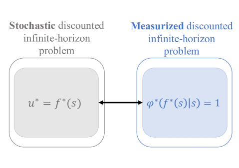
Figure 5: Equivalence between the optimal actions $\varphi^{*}$ of measurized MDP and the optimal actions $u^{*}$ of the original MDP it was lifted from.

The following result shows that the optimal policy of the measurized optimality equations ($\mathcal{M}$-$\alpha$-DCOE) coincides with the optimal policy to ($\alpha$-DCOE); hence it belongs to $\Pi^{D}$ and is attainable.

Theorem 4

The optimal decision rule $\varphi^{*}$ obtained by solving ($\mathcal{M}$-$\alpha$-DCOE) does not depend on the current state distribution $\nu$ and is concentrated around the optimal selector $f^{*}$ attaining the maximum in ($\alpha$-DCOE); that is to say $\varphi^{*}(f^{*}(s)|s)=1$ for all $s\in\mathcal{S}$.

Proof.

Assumptions 2.1 and 2.2 are used in this proof. The optimality equations corresponding to the infinite horizon measurized problem (17) are ($\mathcal{M}$-$\alpha$-DCOE), where

$$\overline{V}^{*}(\nu) =\sup_{\varphi\in\Phi(\nu)}\ \overline{r}(\nu,\varphi)+\alpha\overline{V}^{*}(F(\nu,\varphi)) \forall\nu\in\mathcal{M}_{\mathbb{P}}(\mathcal{S})$$

$$=\sup_{\varphi\in\Phi(\nu)}\ \int_{\mathcal{S}}\int_{\mathcal{U}}\left\{r(s,u)+\alpha\int_{\mathcal{S}}V^{*}(s^{\prime})Q(ds^{\prime}|s,u)\right\}\varphi(du|s)d\nu(s) \forall\nu\in\mathcal{M}_{\mathbb{P}}(\mathcal{S})$$

$$=\sup_{\varphi\in\Phi(\nu)}\ \int_{\mathcal{S}}\int_{\mathcal{U}}\left\{r(s,u)+\alpha\mathbb{E}_{Q}[V^{*}(s^{\prime})|s,u]\right\}\varphi(du|s)d\nu(s) \forall\nu\in\mathcal{M}_{\mathbb{P}}(\mathcal{S})$$

where the second equality comes from Theorem 3 (b) and the definition of the deterministic transition F. Theorem 1 claims that, if Assumptions 2.1 and 2.2 hold, then there exists a selector $f^{*}\in\mathbb{F}$ such that

$$V^{*}(s) =\max_{u\in\mathcal{U}(s)}\left\{r(s,u)+\alpha\mathbb{E}_{Q}[V^{*}(s^{\prime})|s,u]\right\}=r(s,f^{*}(s))+\alpha\mathbb{E}_{Q}[V^{*}(s^{\prime})|s,f^{*}(s)] \forall s\in\mathcal{S},$$

which means that for all $u\in\mathcal{U}(s)$

$$r(s,u)+\alpha\mathbb{E}_{Q}[V^{*}(s^{\prime})|s,u] \leq r(s,f^{*}(s))+\alpha\mathbb{E}_{Q}[V^{*}(s^{\prime})|s,f^{*}(s)]=V^{*}(s) \forall s\in\mathcal{S}.$$

Hence, for any fixed $\nu\in\mathcal{M}_{\mathbb{P}}(\mathcal{S})$ and $\varphi\in\Phi$ we have that

$$\int_{\mathcal{S}}\int_{\mathcal{U}}\left\{r(s,u)+\alpha\mathbb{E}_{Q}[V^{*}(s^{\prime})|s,u]\right\}\varphi(du|s)d\nu(s) \medmath{\leq\int_{\mathcal{S}}\int_{\mathcal{U}}\left\{r(s,f^{*}(s))+\alpha\mathbb{E}_{Q}[V^{*}(s^{\prime})|s,f^{*}(s)]\right\}\varphi(du|s)d\nu(s)}$$

$$=\int_{\mathcal{S}}\left\{r(s,f^{*}(s))+\alpha\mathbb{E}_{Q}[V^{*}(s^{\prime})|s,f^{*}(s)]\right\}d\nu(s)$$

$$=\int_{\mathcal{S}}\int_{\mathcal{U}}\left\{r(s,u)+\alpha\mathbb{E}_{Q}[V^{*}(s^{\prime})|s,u)]\right\}\varphi^{*}(du|s)d\nu(s),$$

where $\varphi^{*}\in\Phi$ is the stochastic kernel concentrated around the selector as $\varphi^{*}(f^{*}(s)|s)=1$ for all $s\in\mathcal{S}$. Therefore,

$$\sup_{\varphi\in\Phi(\nu)}\int_{\mathcal{S}} \int_{\mathcal{U}}\left\{r(s,u)+\alpha\mathbb{E}_{Q}[V^{*}(s^{\prime})|s,u]\right\}\varphi(du|s)d\nu(s) \forall\nu\in\mathcal{M}_{\mathbb{P}}(\mathcal{S})\hskip 56.9055pt$$

$$\leq\sup_{\varphi\in\Phi}\int_{\mathcal{S}}\int_{\mathcal{U}}\left\{r(s,f^{*}(s))+\alpha\mathbb{E}_{Q}[V^{*}(s^{\prime})|s,f^{*}(s)]\right\}\varphi^{*}(du|s)d\nu(s) \forall\nu\in\mathcal{M}_{\mathbb{P}}(\mathcal{S})\hskip 56.9055pt$$

$$=\overline{r}(\nu,\varphi^{*})+\alpha\overline{V}^{*}(F(\nu,\varphi^{*}))=\overline{V}^{*}(\nu) \forall\nu\in\mathcal{M}_{\mathbb{P}}(\mathcal{S})\hskip 56.9055pt\square$$

As a consequence, we can replace the supremum by a maximum in ($\mathcal{M}$-$\alpha$-DCOE), over $\varphi\in\Phi$ independently of $\nu$.

5 An algebraic procedure for lifting the stochastic optimality equations

In this section, we provide an intuitive method for measurizing the stochastic MDP to the measure-valued framework. Figure 6 outlines the process.

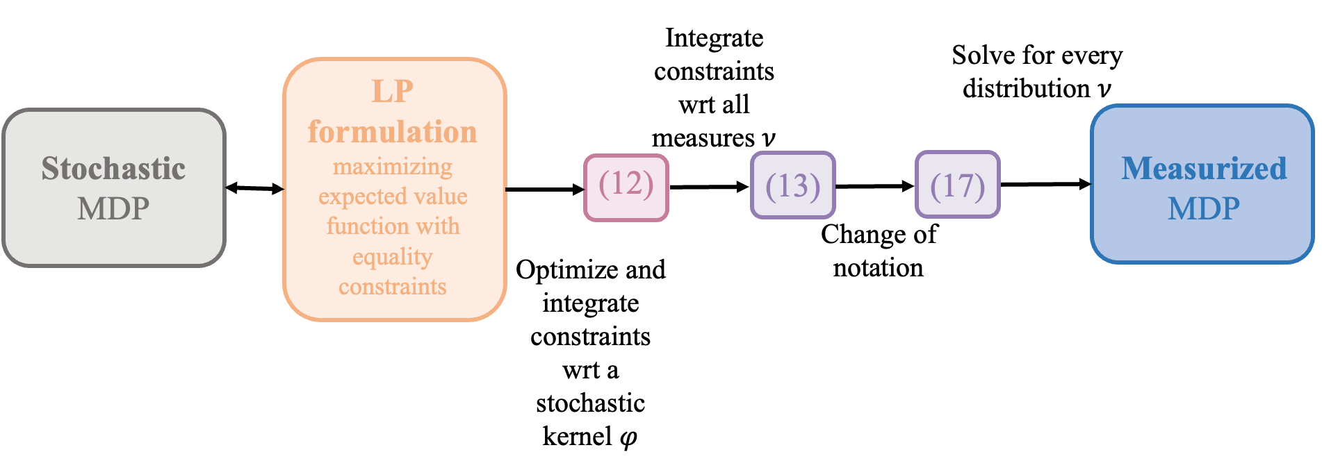
Figure 6: Illustration of the measurizing process; i.e. how one can intuitively lift any stochastic MDP to the measure-valued framework.

The following lemma provides a reformulation of the optimality equations ($\alpha$-DCOE). This reformulation arises by writing the LP formulation with equality constraints, and integrating these in the action space $\mathcal{U}$ with respect to a stochastic kernel $\varphi\in\Phi$ that is optimized, where $\Phi$ is as in (3)

Lemma 1

Let $f^{*}$ and $V^{*}(\cdot)$ be the optimal selector and the optimal pointwise maximal solution to ($\alpha$-DCOE), respectively. Let $(\tilde{V},\tilde{\varphi})$ denote an optimal solution to

$$\sup_{\begin{subarray}{c}\varphi\in\Phi\\ V\in\mathcal{V}(\mathcal{S})\end{subarray}} \ \int_{\mathcal{S}}V(s)d\nu_{0}(s)$$ (22)

s.t. $$\ \ V(s)=\int_{\mathcal{U}}r(s,u)\varphi(du|s)+\alpha\int_{\mathcal{U}}\mathbb{E}_{Q}\left[V(s^{\prime})|s,u\right]\varphi(du|s)\qquad\qquad\forall s\in\mathcal{S}.$$

Then $\tilde{\varphi}(f^{*}(s)|s)=1$ and $\tilde{V}(s)=V^{*}(s)$ $\nu_{0}$-almost everywhere (a.e.).

Proof.

We first show that $(V^{*},\varphi^{*})$, where $\varphi^{*}$ is concentrated around $f^{*}$, is a feasible solution to (22). From Theorem 1 (which makes use of Assumptions 2.1 and 2.2) we know that the optimal value function in ($\alpha$-DCOE) is given by a selector $f^{*}\in\mathbb{F}$, having

$$V^{*}(s) =\ r(s,f^{*}(s))+\alpha\mathbb{E}_{Q}\left[V^{*}(s^{\prime})|s,f^{*}(s)\right] \forall s\in\mathcal{S}$$

$$=\int_{\mathcal{U}}\left\{r(s,u)+\alpha\mathbb{E}_{Q}\left[V^{*}(s^{\prime})|s,u\right]\right\}\varphi^{*}(du|s) \forall s\in\mathcal{S}$$

Therefore, $(V^{*},\varphi^{*})$ is feasible.

We now show that $\tilde{V}(s)=V^{*}(s)$ $\nu_{0}$-a.e by contradicition. Assume this is not true; then there exists a set $\tilde{\mathcal{S}}\in\mathcal{B}(\mathcal{S})$ such that $\nu_{0}(\tilde{\mathcal{S}})>0$ and $\tilde{V}(s)\neq V^{*}(s)$ for all $s\in\tilde{\mathcal{S}}$. Theorem 1 and Lemma 4.2.7 in Hernández-Lerma and Lasserre (1996) entail that $V^{*}\in\mathcal{V}(\mathcal{S})$ is the unique bounded solution to ($\alpha$-DCOE) (see Note 4.2.1 in Hernández-Lerma and Lasserre (1996) for more details on this), thus

$$V^{*}(s) =\sup_{f\in\mathbb{F}}\ \left\{r(s,f(s))+\alpha\mathbb{E}_{Q}\left[V^{*}(s^{\prime})|s,f(s)\right]\right\} \forall s\in\mathcal{S}$$

$$=\sup_{\varphi\in\Phi}\ \int_{\mathcal{U}}\left\{r(s,u)+\alpha\mathbb{E}_{Q}\left[V^{*}(s^{\prime})|s,u\right]\right\}\varphi(du|s) \forall s\in\mathcal{S}$$

$$\geq\int_{\mathcal{U}}r(s,u)\varphi(du|s)+\alpha\int_{\mathcal{U}}\mathbb{E}_{Q}\left[V(s^{\prime})|s,u\right]\varphi(du|s) \forall s\in\mathcal{S}$$

$$=\tilde{V}(s)\qquad \forall s\in\mathcal{S}$$

This implies that $V^{*}(s)>\tilde{V}(s)$ for all $s\in\tilde{\mathcal{S}}$. Therefore

$$\int_{\mathcal{S}}V^{*}(s)d\nu_{0}(s)>\int_{\mathcal{S}}\tilde{V}(s)d\nu_{0}(s),$$

contradicting the optimality of $\tilde{V}(\cdot)$. As a consequence, the optimal solution to (22) needs to equal $V^{*}(\cdot)$ $\nu_{0}$-a.e. $\square$

Program (22) is a relaxation of the optimality equations ($\alpha$-DCOE) since it enlarges the space of solutions of the latter. Because the objective function of the former only emphasizes states that are reachable from the initial state distribution, its optimal solutions may assign lower values to unreachable states. This means that the optimal policies may also differ for those unreachable states. The following lemma shows that aggregating the constraints in Problem (22) over any measure $\nu\in\mathcal{M}(\mathcal{S})$ allows one to retrieve the optimal decision rule and value function of ($\alpha$-DCOE).

Lemma 2

Let $f^{*}$ and $V^{*}(\cdot)$ be the optimal selector and the optimal pointwise maximal solution to ($\alpha$-DCOE), respectively. Let $(V^{\prime},\varphi^{\prime})$ denote an optimal solution to

$$\sup_{\begin{subarray}{c}\varphi\in\Phi\\ V\in\mathcal{V}(\mathcal{S})\end{subarray}} \ \int_{\mathcal{S}}V(s)d\nu_{0}(s)$$ (23)

s.t. $$\int_{\mathcal{S}}V(s)d\nu(s)=\int_{\mathcal{S}}\int_{\mathcal{U}}\left\{r(s,u)+\alpha\mathbb{E}_{Q}\left[V(s^{\prime})|s,u\right]\right\}\varphi(du|s)d\nu(s)\qquad\qquad\forall\nu\in\mathcal{M}_{\mathbb{P}}(\mathcal{S}).$$

Then $\varphi^{\prime}(f^{*}(s)|s)=1$ and $V^{\prime}(s)=V^{*}(s)$ $\nu_{0}$-almost everywhere.

Proof.

It suffices to prove that any optimal solution to (23) equals any optimal solution to (22) when evaluated at any state $s$ reachable from $\nu_{0}$. Since the objective function of both problems is the same, it suffices to prove that:

1. Any feasible solution to (23) is also a solution to (22)

2. Any feasible solution to (22) is also a solution to (23):

Point (i) is true as the Dirac measure $\delta_{s}$ belongs to $\mathcal{M}_{\mathbb{P}}(\mathcal{S})$ for all $s\in\mathcal{S}$.

To show (ii), let $(V^{\prime},\varphi^{\prime},)$ be a feasible solution to (22). Then

$$V^{\prime}(s)=\int_{\mathcal{U}}\left(r(s,u)+\alpha\mathbb{E}_{Q}\left[V^{\prime}(s^{\prime})|s,u\right]\right)\varphi^{\prime}(du|s)\qquad\forall s\in\mathcal{S}$$ (24)

and as a consequence we get

$$\int_{\mathcal{S}}V^{\prime}(s)d\nu(s)=\int_{\mathcal{S}}\int_{\mathcal{U}}\left(r(s,u)+\alpha\mathbb{E}_{Q}\left[V^{\prime}(s^{\prime})|s,u\right]\right)\varphi^{\prime}(du|s)d\nu(s)\qquad\forall\nu\in\mathcal{M}_{\mathbb{P}}(\mathcal{S})$$

which is (23). $\square$

Since we are optimizing $V(\cdot)$ in the space of bounded measurable functions on $\mathcal{S}$, $\mathcal{V}(\mathcal{S})$, the objective in (23) is well defined and bounded. Denote

$$\overline{V}(\nu):=\int_{\mathcal{S}}V(s)d\nu(s)=\mathbb{E}_{\nu}[V(s)]<\infty;$$ (25)

then $\overline{V}\in\mathcal{V}(\mathcal{M}_{\mathbb{P}}(\mathcal{S}))$, where $\mathcal{V}(\mathcal{M}_{\mathbb{P}}(\mathcal{S}))$ denotes the space of bounded measurable functions in the space of distributions $\mathcal{M}_{\mathbb{P}}(\mathcal{S})$. Then Problem (23) can be rewritten as

$$\sup_{\begin{subarray}{c}\varphi\in\Phi\\ \overline{V}\in\mathcal{V}(\mathcal{M}_{\mathbb{P}}(\mathcal{S}))\end{subarray}} \ \overline{V}(\nu_{0})$$ (26)

s.t. $$\ \overline{V}(\nu)=\overline{r}(\nu,\varphi)+\alpha\int_{\mathcal{S}}\int_{\mathcal{U}}\mathbb{E}_{Q}\left[V(s^{\prime})|s,u\right]\varphi(du|s)d\nu(s)\qquad\qquad\forall\nu\in\mathcal{M}_{\mathbb{P}}(\mathcal{S})$$

Now decompose the expectation in (26) as

$$\int_{\mathcal{S}}\int_{\mathcal{U}}\mathbb{E}_{Q}\left[V(s^{\prime})|s,u\right]\varphi(du|s)d\nu(s) =\int_{\mathcal{S}}\int_{\mathcal{U}}\int_{\mathcal{S}}V(s^{\prime})Q(ds^{\prime}|s,u)\varphi(du|s)d\nu(s)$$

$$=\int_{\mathcal{S}}V(s^{\prime})\int_{\mathcal{U}}\int_{\mathcal{S}}Q(ds^{\prime}|s,u)\varphi(du|s)d\nu(s)$$

$$=\int_{\mathcal{S}}V(s^{\prime})dF(\nu,\varphi)(s^{\prime})$$

$$=\overline{V}(F(\nu,\varphi))=\overline{V}(\nu^{\prime}),$$

where $F$ is as defined in (6) and Fubini’s Theorem ensures that the order of integration can be switched. This new notation is consistent with the notion of the optimal measurized value function being the expected value of the optimal original value function, as demonstrated in Theorem 3. Hence we use the new notation to rewrite Problem (23) as

$$\sup_{\begin{subarray}{c}\varphi\in\Phi\\ \overline{V}\in\mathcal{V}(\mathcal{M}_{\mathbb{P}}(\mathcal{S}))\end{subarray}} \ \overline{V}(\nu_{0})$$ (27)

s.t. $$\ \overline{V}(\nu)=\overline{r}(\nu,\varphi)+\alpha\overline{V}(F(\nu,\varphi))\qquad\qquad\forall\nu\in\mathcal{M}_{\mathbb{P}}(\mathcal{S}).$$

Although this problem resembles the measurized LP formulation ($\mathcal{M}$-LP), it is essentially different. First, we do not have as many constraints as feasible state-action pairs. Instead, we are optimizing over a unique stochastic kernel $\varphi$. This means that the optimal solution $\tilde{\varphi}$ to (27) is one action rather than the optimal selector $\overline{f}^{*}$ to ($\mathcal{M}$-$\alpha$-DCOE), that allows actions $\varphi$ to depend on state-distributions $\nu$. Second, we are optimizing $\varphi$ over $\Phi$ rather than a set $\Phi(\nu_{0})$ that may be contingent on $\nu_{0}$. This is a direct consequence of the first point since the one $\varphi$ chosen has to work for all reachable $\nu$. Third, this formulation has equality constraints rather than inequality constraints. Finally, we are maximizing rather than minimizing. Therefore, moving from (27) to ($\mathcal{M}$-$\alpha$-DCOE) is not straightforward. However, because we are optimizing $\overline{V}(\cdot)$ and $\varphi$ for $\nu_{0}$, the equality constraint evaluated at $\nu_{0}$ intuitively gives rise to the definition of measurized value function in (10) but requiring a constant decision rule

$$\overline{V}^{*}(\nu_{0})=\sup_{\varphi\in\Phi}\sum_{t=0}^{\infty}\alpha^{t}\overline{r}(\nu_{t},\varphi).$$

Theorem 4 ensures that this is equivalent to (10), thus giving rise to the optimal measurized value function and optimal measurized decision rules, that can also be retrieved by solving ($\mathcal{M}$-$\alpha$-DCOE) with $\Phi(\nu)=\Phi$ for all probability measures $\nu$.

6 Connection to the Linear Programming formulation of the original MDP

In this section we demonstrate that the dual variables $\zeta$ of the LP formulation (LP) can be interpreted as a discounted sum of state distributions $\{\nu_{t}\}_{t\geq 0}$ and measurized controls $\{\varphi_{t}\}_{t\geq 0}$. More specifically, we show that

$$\zeta(\mathcal{A},\mathcal{D})=\sum_{t=1}^{\infty}\alpha^{t}\int_{\mathcal{S}}\varphi_{t}(\mathcal{D}|s)d\nu_{t}(s).$$

This allows us to think of measurizing as dualizing the standard LP formulation of ($\alpha$-DCOE) and performing some changes of variables, as illustrated in Figure 7.

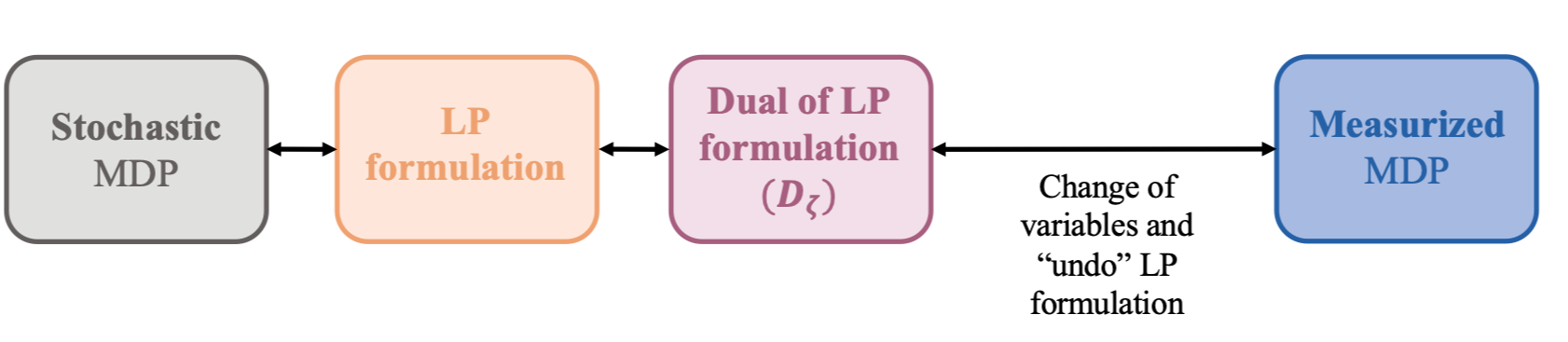
Figure 7: Illustration of the relationship between the LP formulation of the stochastic MDP and the measurized MDP. This offers an alternative recipe for measurizing any MDP.

More specifically, the change of variables is performed through the joint state-action distribution

$$\gamma_{t}(\mathcal{A},\mathcal{D}):=\int_{\mathcal{A}}\int_{\mathcal{D}}\varphi_{t}(du|s)d\nu_{t}(s)\qquad\forall\mathcal{A}\in\mathcal{B}(\mathcal{S}),\mathcal{D}\in\mathcal{B}(\mathcal{U}).$$ (28)

Note that $\gamma(\cdot,\mathcal{S})$ coincides with the overall distribution of actions (12). Figure 8 visually demonstrates the process of implementing this change of variables. In the next section, we establish that this change can be executed without compromising optimality. We then will establish the connection between the measurized value function and the dual problem (D_ζ).

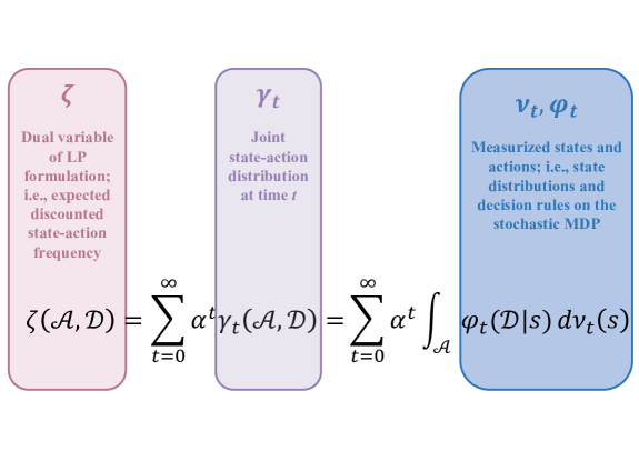
Figure 8: Visual representation of the relationship between the dual variables $\zeta$ of the LP formulation of the stochastic MDP, the joint state-action distribution at time $t$, $\gamma_{t}$, and the measurized states and actions.

6.1 Decomposing expected discounted state-action frequencies into measurized states and actions

For a given pair $(\nu_{t},\varphi_{t})\in\mathcal{M}_{\mathbb{P}}(\mathcal{S})\times\mathcal{K}(\mathcal{U}|\mathcal{S})$, there exists a unique joint distribution $\gamma_{t}\in\mathcal{M}_{\mathbb{P}}(\mathcal{S},\mathcal{U})$ such that (28) holds almost surely with respect to $(\nu_{t},\varphi_{t})$. Our first goal is to demonstrate that for given $\gamma_{t},\nu_{t}$ there exists a unique kernel $\varphi_{t}$ satisfying (28). To ease notation, denote the complement of a set $\mathcal{A}$ as $\mathcal{A}^{c}$ and define

$$\Xi=\left\{\gamma\in\mathcal{M}_{\mathbb{P}}(\mathcal{S},\mathcal{U}):\int_{s\in\mathcal{A}}\int_{\mathcal{U}(s)^{c}}\gamma(ds,du)=0\ \ \forall\mathcal{A}\in\mathcal{B}(\mathcal{S})\right\}.$$ (29)

The following lemma ensures that, under certain conditions, there is a one-on-one relationship between the probability measure $\gamma\in\Xi$ and the pair $(\nu,\varphi)\in\mathcal{M}_{\mathbb{P}}(\mathcal{S})\times\Phi$.

Lemma 3

Assume that $(\mathcal{S},\mathcal{B}(\mathcal{S}),\nu)$ and $(\mathcal{U}(s),\mathcal{B}(\mathcal{U}(s)),\varphi(\cdot|s))$ for every $s\in\mathcal{S}$ are complete measure spaces. For all $t$, let $\nu_{t}\in\mathcal{M}_{\mathbb{P}}(\mathcal{S})$ and $\gamma_{t}\in\Xi$ be probability measures such that

$$\gamma_{t}(\mathcal{A},\mathcal{U})=\nu_{t}(\mathcal{A}),\quad\forall\mathcal{A}\in\mathcal{B}(\mathcal{S}).$$ (30)

Then there exists a unique stochastic kernel $\varphi\in\Phi$ such that (28) holds.

Proof.

Recall that $\Phi=\{\varphi\in\mathcal{K}(\mathcal{U}|\mathcal{S}):\ \varphi(\mathcal{U}(s)|s)=1\ \forall s\in\mathcal{S}\}$ and pick any $\phi\in\Phi$. First, we prove that $\gamma_{t}(\mathcal{A},\cdot)$ is absolutely continuous with respect to measure

$$\eta_{t}(\mathcal{A},\mathcal{D})=\int_{\mathcal{A}}\phi(\mathcal{D}|s)d\nu_{t}(s)\qquad\mathcal{D}\in\mathcal{B}(\mathcal{U})$$

for all $\mathcal{A}\in\mathcal{B}(\mathcal{S})$. We use the fact that $\eta_{t}(\mathcal{A},\mathcal{D})=0$ implies that either

1. $\mathcal{D}\bigcap\left(\cup_{s\in\mathcal{A}}\mathcal{U}(s)\right)=\emptyset$, or

2. $\nu_{t}(\mathcal{A})=0$

In case (i), $\gamma_{t}(\mathcal{A},\mathcal{D})=0$ by definition of $\Xi$. In case (ii), completeness yields

$$\gamma_{t}(\mathcal{A},\mathcal{D})\leq\gamma_{t}(\mathcal{A},\mathcal{U})=\nu_{t}(\mathcal{A})$$ (31)

and hence $\gamma_{t}(\mathcal{A},\mathcal{D})=0$ if $\nu_{t}(\mathcal{A})=0$. Then the Radon-Nikodym theorem states that for all $\mathcal{A}\in\mathcal{B}(\mathcal{S})$ there exists a measurable function $g:\mathcal{S}\times\mathcal{U}\rightarrow[0,\infty)$ such that

$$\gamma_{t}(\mathcal{A},\mathcal{D})=\int_{\mathcal{A}}\int_{\mathcal{D}}g(s,u)\eta_{t}(ds,du)=\int_{\mathcal{D}}\int_{\mathcal{A}}g(s,u)\phi(du|s)d\nu_{t}(s).$$

and $g$ is unique $\eta_{t}$-almost everywhere.

Second, we prove that the stochastic kernel defined as

$$\varphi_{t}(\mathcal{D}|s)=\int_{\mathcal{D}}g(s,u)\phi(du|s)\qquad\forall s\in\mathcal{S},\forall\mathcal{D}\in\mathcal{B}(\mathcal{U})$$ (32)

belongs to $\Phi$. Note that Equation (30) implies that

$$\gamma_{t}(\mathcal{A},\mathcal{U})=\int_{\mathcal{U}}\int_{\mathcal{A}}g(s,u)\phi(du|s)d\nu_{t}(s)=\nu_{t}(\mathcal{A}).$$

Exchanging the order of integration we have that

$$\int_{\mathcal{U}}g(s,u)\phi(du|s)=1\qquad\forall s\in\mathcal{S},$$

and because $\gamma_{t}\in\Xi$ and the measure spaces are complete we also have that

$$\int_{\mathcal{D}}\int_{\mathcal{A}}g(s,u)\phi(du|s)d\nu_{t}(s)=0\qquad\forall\mathcal{D}\subseteq\left(\cup_{s\in\mathcal{A}}\mathcal{U}(s)\right)^{c}$$

which proves that $\varphi_{t}\in\Phi$. Since $g$ is unique $\eta_{t}$-a.e., this means that there exists a stochastic kernel $\varphi_{t}\in\Phi$ that is unique $\eta_{t}$-a.e and is defined as in (32) such that (28) holds. $\square$

Denote $\Gamma=\{\gamma_{t}\}_{t\geq 0}$ and define the possible path of joint state-action distributions starting at $\nu_{0}$ as

$$\Omega(\nu_{0}):=\left\{\Gamma:\right.\ \gamma_{t}\in\mathcal{M}_{\mathbb{P}}(\mathcal{S},\mathcal{U})\cap\Xi\ \forall t\geq 0,\ \ \gamma_{0}(\cdot,\mathcal{U})=\nu_{0}(\cdot),\left.\gamma_{t}(\cdot,\mathcal{U})=\int_{\mathcal{S}}\int_{\mathcal{U}}Q(\cdot|s,u)d\gamma_{t-1}(s,u)\ \forall t\geq 1\right\}.$$

The following proposition proves that given an initial state distribution $\nu_{0}$ and a sequence $\Gamma\in\Omega(\nu_{0})$, there exist stochastic kernels $\varphi_{t}\in\Phi$ for all $t\geq 0$ such that there is a one-on-one relationship between $\gamma_{t}$ and $(\nu_{t},\varphi_{t})$ for all $t\geq 0$, where $\nu_{t}$ obeys the transition law F for all $t\geq 1$.

Proposition 3

Assume that $(\mathcal{S},\mathcal{B}(\mathcal{S}),\nu)$ and $(\mathcal{U}(s),\mathcal{B}(\mathcal{U}(s)),\varphi(\cdot|s))$ are complete measure spaces for every $s\in\mathcal{S}$. Given a $\nu_{0}$ and a sequence $\Gamma\in\Omega(\nu_{0})$, there exists a unique sequence of stochastic kernels $\{\varphi_{t}\}_{t\geq 0}$ and a unique sequence of probability measures $\{\nu_{t}\}_{t\geq 0}$ verifying $\varphi_{t}\in\Phi$ and $\nu_{t+1}=F(\nu_{t},\varphi_{t})$ for all $t\geq 0$ such that (28) holds.

Proof.

We prove this by induction.

$\bullet$t=0: Since $\gamma_{0}\in\Xi$ and (30) holds, we can apply Lemma 3 to prove that there exists a unique kernel $\varphi_{0}\in\Phi$ such that (28) holds.

$\bullet$t=T: Assume true; i.e., assume (28) holds for $\nu_{T}$.

$\bullet$t=T+1: Since $\Gamma\in\Omega(\nu_{0})$, then $\gamma_{T+1}\in\Xi$. From Lemma 3, it suffices to prove that $\gamma_{T+1}(\mathcal{A},\mathcal{U})=\nu_{T+1}(\mathcal{A})$, where $\nu_{T+1}=F(\nu_{T},\varphi_{T})$, to have (28). Because $\Gamma\in\Omega(\nu_{0})$, we have that

$$\gamma_{T+1}(\mathcal{A},\mathcal{U}) =\int_{\mathcal{S}}\int_{\mathcal{U}}Q(\mathcal{A}|s,u)d\gamma_{T}(s,u)$$

$$=\int_{\mathcal{S}}\int_{\mathcal{U}}Q(\mathcal{A}|s,u)\varphi_{T}(du|s)d\nu_{T}(s)=F(\nu_{T},\varphi_{T})(\mathcal{A})$$

$$=\nu_{T+1}(\mathcal{A})$$

where the second equality comes from the fact that $\gamma_{T}(\mathcal{A},\mathcal{D})=\int_{\mathcal{A}}\varphi_{T}(\mathcal{D}|s)d\nu_{T}(s)$ for all $\mathcal{A}\in\mathcal{B}(\mathcal{S}),\ \mathcal{D}\in\mathcal{B}(\mathcal{U})$. $\square$

6.2 The measurized problem as the dual of the LP formulation

Using Theorem 1, Theorem 3 and Proposition 3, one can perform the change of variables (28) in the discounted infinite-horizon problem (10), yielding

$$\overline{V}^{*}(\nu_{0})=\sup_{\Gamma\in\Omega(\nu_{0})}\ \sum_{t=0}^{\infty}\alpha^{t}\mathbb{E}_{\gamma_{t}}\left[r(s,u)\right]\qquad\nu_{0}\in\mathcal{M}_{\mathbb{P}}(\mathcal{S}).$$ (33)

Because the reward function $r$ does not depend on time $t$, intuitively one could perform in (33) the following change of variables

$$\zeta(\mathcal{A},\mathcal{D})=\sum_{t=0}^{\infty}\alpha^{t}\gamma_{t}(\mathcal{A},\mathcal{D})\qquad\forall\mathcal{A}\in\mathcal{B}(\mathcal{S}),\mathcal{D}\in\mathcal{B}(\mathcal{U}). \zeta$$ ()

Recall that $\zeta(\mathcal{S},\mathcal{U})=1/(1-\alpha)$, so $\zeta$ is not a probability measure. Performing change of variables ($\zeta$) would lead to an optimization problem

$$\overline{V}^{*}(\nu_{0})=\sup_{\zeta\in Z(\nu_{0})}\ \int_{\mathcal{S}}\int_{\mathcal{U}}r(s,u)d\zeta(s,u)\qquad\nu_{0}\in\mathcal{M}_{\mathbb{P}}(\mathcal{S}),$$ (34)

where the set $Z(\nu_{0})$ gathers the transition law of $\gamma_{t}$ and thus $\nu_{t}$, having

$$Z(\nu_{0}):= \left\{\zeta\in\mathcal{M}_{+}(\mathcal{S},\mathcal{U}):\ \zeta(\mathcal{A},\mathcal{U}(\mathcal{A})^{c})=0\ \ \forall\mathcal{A}\in\mathcal{B}(\mathcal{S}),\phantom{\int_{\mathcal{S}}}\right.$$

$$\left.\quad\zeta(\mathcal{A},\mathcal{U})=\nu_{0}(\mathcal{A})+\alpha\int_{\mathcal{S}}\int_{\mathcal{U}}Q(\mathcal{A}|s,u)d\zeta(s,u)\ \ \forall\mathcal{A}\in\mathcal{B}(\mathcal{S})\right\}.$$

With this specification, Problem (34) is actually the dual (D_ζ) of the LP formulation of the stochastic MDP. This means that, if we can perform the change of variables ($\zeta$) without loss of optimality, one can view the measurized MDP as equivalent to the dual of the stochastic MDP. The following proposition shows this.

Proposition 4

Let $\zeta^{*}$ be the optimal solution to (D_ζ). Let $\overline{V}^{*}(\cdot)$ and $\varphi^{*}$ be the optimal measurized value function and decision rule solving ($\mathcal{M}$-$\alpha$-DCOE). Denote the optimal state-distribution path that $\varphi^{*}$ gives rise to as $\Upsilon^{*}=\{\nu_{t}^{*}\}_{t\geq 0}$, where $\nu_{0}^{*}$ coincides with the initial state distribution $\nu_{0}$. Then:

• $\overline{V}^{*}(\nu_{0})$ coincides with the optimal objetive of the dual problem (D_ζ).

• Without loss of optimality we can assume that $\zeta^{*}(\mathcal{A},\mathcal{D})=\sum_{t=0}^{\infty}\alpha^{t}\int_{\mathcal{A}}\varphi^{*}(\mathcal{D}|s)d\nu_{t}^{*}(s)$ for all $\mathcal{A}\in\mathcal{B}(\mathcal{S})$, $\mathcal{D}\in\mathcal{B}(\mathcal{U})$.

Proof.

This proof adopts Assumptions 2.1, 2.2 and 2.3.

The proof of (a) is straightforward, since we have that

$$\overline{V}^{*}(\nu_{0})=\int_{S}V^{*}(s)d\nu_{0}(s)=\int_{\mathcal{S}}\int_{\mathcal{U}}r(s,u)d\zeta^{*}(s,u),$$

where the first equality comes from Theorem 3.(b) and the second equality is given by Theorem 2.

To show (b), we construct the following measure for any initial state distribution $\nu_{0}\in\mathcal{M}_{\mathbb{P}}(\mathcal{S})$

$$\tilde{\zeta}(\mathcal{A},\mathcal{D}):=\sum_{t=0}^{\infty}\alpha^{t}\int_{\mathcal{A}}\varphi^{*}(\mathcal{D}|s)d\nu_{t}^{*}(s),\qquad\forall\ \mathcal{A}\in\mathcal{B}(\mathcal{S}),\ \mathcal{D}\in\mathcal{B}(\mathcal{U}).$$

To prove (b), it suffices to show that

• $\tilde{\zeta}$ is feasible to (D_ζ).

• $\tilde{\zeta}$ gives the same objective value as $\zeta^{*}$ in (D_ζ); i.e. $\int_{\mathcal{S}}\int_{\mathcal{U}}r(s,u)d\tilde{\zeta}(s,u)=\int_{\mathcal{S}}\int_{\mathcal{U}}r(s,u)d\zeta^{*}(s,u)$.

$\bullet$ We start by proving (i):

$$\tilde{\zeta}(\mathcal{A},\mathcal{U}) =\sum_{t=0}^{\infty}\alpha^{t}\int_{\mathcal{A}}\varphi^{*}(\mathcal{U}|s)d\nu_{t}^{*}(s)=\sum_{t=0}^{\infty}\nu_{t}^{*}(\mathcal{A})$$

$$=\nu_{0}^{*}(\mathcal{A})+\sum_{t=1}^{\infty}\alpha^{t}F(\varphi^{*},\nu^{*}_{t-1})(\mathcal{A})$$

$$=\nu_{0}^{*}(\mathcal{A})+\sum_{t=1}^{\infty}\alpha^{t}\int_{\mathcal{S}}\int_{\mathcal{U}}Q(\mathcal{A}|s,u)\varphi^{*}(du|s)d\nu^{*}_{t-1}(s)$$

$$=\nu_{0}^{*}(\mathcal{A})+\alpha\int_{\mathcal{S}}\int_{\mathcal{U}}Q(\mathcal{A}|s,u)\sum_{t=0}^{\infty}\alpha^{t}\varphi^{*}(du|s)d\nu^{*}_{t}(s)$$

$$=\nu_{0}^{*}(\mathcal{A})+\alpha\int_{\mathcal{S}}\int_{\mathcal{U}}Q(\mathcal{A}|s,u)d\tilde{\zeta}(s,u),$$

where the fifth equality comes from the Monotone Convergence Theorem. In addition,

$$\tilde{\zeta}(\mathcal{A},\mathcal{U}(\mathcal{A})^{c})=\sum_{t=0}^{\infty}\alpha^{t}\int_{\mathcal{A}}\varphi^{*}(\mathcal{U}(\mathcal{A})^{c}|s)d\nu_{t}^{*}(s)=0$$

because $\varphi^{*}(\mathcal{U}(s)|s)=1$ for all $s\in\mathcal{S}$. Therefore, $\tilde{\zeta}\in\mathcal{M}_{+}(\mathbb{K})$ and it fulfills the constraint in (D_ζ).

$\bullet$ We now prove (ii):

$$\int_{\mathcal{S}}\int_{\mathcal{U}}r(s,u)d\zeta^{*}(s,u) =\overline{V}^{*}(\nu_{0})=\sup_{\begin{subarray}{c}\varphi_{t}\in\Phi,\\ t\geq 0\end{subarray}}\mathbb{E}_{\nu_{0}}^{\pi}\left[\sum_{t=0}^{\infty}\alpha^{t}r(s_{t},u_{t})\right]$$

$$=\int_{\mathcal{S}}\int_{\mathcal{U}}\sum_{t=0}^{\infty}\alpha^{t}r(s,u)\varphi^{*}(du|s)d\nu_{t}^{*}(s)$$

$$=\int_{\mathcal{S}}\int_{\mathcal{U}}r(s,u)d\tilde{\zeta}(s,u),$$

where the first equality comes from (a) and the rest from plugging the optimal decision rule $\varphi^{*}$ and the optimal path of state distributions $\Upsilon^{*}$ in the measurized discounted infinite horizon expression (17). $\square$

7 Concluding remarks and extensions

In this paper, we have rigorously established a framework for lifted MDPs in the space of measures. We provide an algebraic lifting procedure that can be applied to any standard MDP and show that this measurizing procedure transforms any stochastic MDP into a deterministic process.

The so-called measurized MDPs are a special case of measure-valued MDPs, which have seldom been the focus of extensive study, with notable exceptions being MFMDPs and POMDPs. Recently, Bäuerle (2023) demonstrated that the value function of classical MFMDPs converges to the measurized value function $\overline{V}^{*}(\cdot)$ as the number of agents in the mean-field game increases, yielding to a deterministic process in the absence of random shocks. Our approach generalizes these findings to any standard MDP, broadening the applicability of the model and potentially facilitating the analysis of MFMDPs. Another key advantage of operating within the measurized framework is that it enables the consideration of a diverse set of constraints and value function approximations that are beyond reach within the standard framework. For instance, it allows us to model moment, CVaR, and other risk constraints—capabilities that contrast with conventional approaches found in the literature operating within the standard framework.

Our primary focus has been on bridging standard and measurized MDPs. We prove that measurizing is equivalent to dualizing and performing a change of variables on the LP formulation of the discounted optimality equations. The novel change of variables executed is based on the Radon-Nikodym derivative of the expected discounted state-action frequencies $\zeta$ discussed in Chapter 6 of Hernández-Lerma and Lasserre (1996). Such a change of variables decomposes $\zeta$ in time-dependent state distributions and stochastic kernels in the action space. Moreover, it allows us to retrieve information on how often an action is implemented. Indeed, take distribution $\gamma_{t}$ defined in (28). When evaluated over the entire state space $\mathcal{S}$, this measure coincides with distribution (12), which indicates how often a particular decision is made at period $t\geq 0$, potentially pointing out the actions that should be streamlined. Future work may exploit this particularity of the measurized framework to partition the state space according to the actions that are more likely to be implemented. Furthermore, this may also facilitate the study and understanding of structured policies, providing yet another interesting avenue for future applications.

Another insight is the interpretation of the measurized value function as the expected value of the stochastic value function. In fact, we show that the average of the stochastic value function evaluated at an i.i.d. sample of states converges to the measurized value function of their sampling distribution. This allows us to interpret a measurized MDP as solving over infinite realizations of a standard (stochastic) MDP.

Future works applying the measurized framework in the modelling and resolution of MDP problems are especially promising within weakly coupled MDPs. For instance, in Adelman and Olivares-Nadal (2024b) the authors leverage the measurized framework to facilitate a timewise dualization of the linking constraints in weakly coupled MDPs. Finally, more theoretical works may focus on extending the measurized perspective to other frameworks within the MDP field. In particular, in Adelman and Olivares-Nadal (2024a) the authors extend the measurized framework to the long-run average reward case.

Appendix

Appendix A Additional definitions and theoretical results from Hernández-Lerma and Lasserre (1996)

Definition 7 (sup-compact)

A function $g:\mathbb{K}\to\mathbb{R}$ is said to be upper sup-compact on $\mathbb{K}$ if the set

$$\{u\in\mathcal{U}(s):\ g(s,u)\geq c\}$$

is compact for every $s\in\mathcal{S}$ and $c\in\mathbb{R}$.

Definition 8 (upper semicontinuous)

Let $\mathcal{X}$ be a metric space and $g:\mathcal{X}\to\mathbb{R}\cup\{+\infty\}$ a function such that $g(x)<\infty$ for all $x\in\mathcal{X}$. Then $g$ is said to be upper semicontinuous at $x\in\mathcal{X}$ if

$$\lim\sup_{n\to\infty}g(x_{n})\geq g(x)$$

for all sequences $\{x_{n}\}_{n\in\mathbb{N}}$ in $\mathcal{X}$ that converge to $x$.

Definition 9 (Strongly continuous kernel)

The stochastic kernel $Q\in\mathcal{K}(\mathcal{S}|\mathbb{K})$ is called strongly continuous if the function $(s,u)\mapsto\int_{\mathcal{S}}g(s^{\prime})Q(ds^{\prime}|s,u)$ is continuous and bounded in $\mathcal{S}$ for every measurable and bounded function $g$.

Proposition 5 (Hernández-Lerma and Lasserre (1996), Proposition A.1)

Let $g$ be a function as in the definition above. Then the following statements are equivalent:

• g is upper semicontinuous

• the set $\{(x,c)\in\mathcal{X}\times\mathbb{R}:\ g(x)\geq c\}$ is closed

• the sets $S_{c}(g):=\{x\in\mathcal{X}:\ g(x)\geq c\}$ are closed for all $c\in\mathbb{R}$.

Proposition 6 (Hernández-Lerma and Lasserre (1996), Proposition A.2)

Let $L(\mathcal{X})$ be the family of all functions on $\mathcal{X}$ that are lower semicontinuous and bounded below. Then $g\in L(\mathcal{X})$ if and only if there exists a sequence $\{g_{n}\}_{n}$ of continuous and bounded functions on $\mathcal{X}$ such that $g_{n}\uparrow g$.

Proposition 7 (Hernández-Lerma and Lasserre (1996), Proposition E.2)

Let $\mu,\mu_{1},\mu_{2}....\in\mathcal{M}{P}(\mathcal{X})$ such that the sequence $\{\mu_{n}\}_{n\in\mathbb{N}}$ converges weakly to $\mu$. If $g:\mathcal{X}\rightarrow\mathbb{R}$ is upper semicontinuous and bounded above, then

$$\lim\sup_{n\to\infty}\int_{\mathcal{X}}g(x)d\mu_{n}(x)\leq\int_{\mathcal{X}}g(x)d\mu(x).$$

In other words, the function $\mu\mapsto\ \int_{\mathcal{X}}g(x)d\mu(x)$ inherits the upper semicontinuity from $g$.

Appendix B The measurized MDP inherits the assumptions from the stochastic MDP

Proof.

A1.(a).i: We first show that $\overline{r}$ is upper bounded. This is straightforward since $r$ is upper bounded, so $\mathbb{E}_{\nu}\mathbb{E}_{\varphi}[r(s,u)]<\infty$ as well.

A1.(a).ii: Second, we prove that $\overline{r}$ is upper semicontinuous. We will use Proposition E.2 in Hernández-Lerma and Lasserre (1996) (corresponding to Proposition 7 in this appendix). Take the joint probability measure $\gamma\in\mathcal{M}{P}(\mathcal{S}\times\mathcal{U})$ from (28). In Section 6 we show that this change of variables can be performed without loss of generality; i.e., for every $\nu\in\mathcal{M}_{\mathbb{P}}(\mathcal{S})$ and $\varphi\in\Phi(\nu)$ there is a unique $\gamma$ verifying (28). One can therefore construct a sequence $\{\gamma_{n}\}_{n\in\mathbb{N}}$ converging weakly to $\gamma$. Since $r$ is upper semicontinuous by assumption, by Proposition E.2 in Hernández-Lerma and Lasserre (1996) we get

$$\lim\sup_{n\to\infty}\int_{\mathcal{S}}\int_{\mathcal{U}}r(s,u)d\gamma_{n}(s,u)\leq\int_{\mathcal{S}}\int_{\mathcal{U}}r(s,u)d\gamma(s,u).$$

Because any pair $(\nu,\gamma)$ is uniquely characterized by a $\gamma$, this shows that $\overline{r}$ is upper semicontinuous.

A1.(a).iii: To finish with Assumption 2.1(a), we need to prove that $\overline{r}$ is sup-compact in $\overline{\mathbb{K}}$. That is to say, we need to show that the set

$$\overline{\mathcal{U}}_{c}(\nu):=\{\varphi\in\Phi(\nu):\ \overline{r}(\nu,\varphi)\geq c\}$$

for every $\nu\in\mathcal{M}_{\mathbb{P}}(\mathcal{S})$ and $c\in\mathbb{R}$. It suffices to prove that $\overline{\mathcal{U}}_{c}(\nu)$ is bounded and closed for every $\nu$. To demonstrate that the set is closed, define the following Total Variation norm in the space of stochastic kernels $\mathcal{K}(\mathcal{U}|\mathcal{S})$

$$TV_{\mathcal{K}}(\varphi,\phi):=\sup_{\begin{subarray}{c}s\in\mathcal{S}\\ \mathcal{A}\in\mathcal{B}(\mathcal{U})\end{subarray}}\left|\varphi(\mathcal{A}|s)-\phi(\mathcal{A}|s)\right|.$$

Given that $\varphi(\cdot|s),\ \phi(\cdot|s)$ are probability measures for any $s\in\mathcal{S}$, we have that $TV_{\mathcal{K}}(\varphi,\phi)\leq 1$ for all $\varphi,\phi\in\mathcal{K}(\mathcal{U}|\mathcal{S})$. Therefore $\mathcal{K}(\mathcal{U}|\mathcal{S})$ is bounded. Since $\Phi(\nu)\subseteq\mathcal{K}(\mathcal{U}|\mathcal{S})$, it is bounded as well.

To show that $\overline{\mathcal{U}}_{c}(\nu)$ is closed, we build on the fact that the function $\varphi\mapsto\int_{\mathcal{S}}r(s,u)\varphi(\mathcal{U}|s)d\nu$ is upper semicontinuous on $\Phi(\nu)$ for every $\nu\in\mathcal{M}_{\mathbb{P}}(\mathcal{S})$. To see this, follow the proof of A1.(a).ii fixing $\nu$. According to Proposition A.1 in Hernández-Lerma and Lasserre (1996) (see Proposition 5 in the appendix), this implies that $\overline{\mathcal{U}}_{c}(\nu)$ is closed. We have this result for every $\nu\in\mathcal{M}_{\mathbb{P}}(\mathcal{S})$.

A1.(b): We now show that $\overline{Q}$ inherits weak continuity from the strong continuity of $Q$. We need to prove that

$$(\nu,\varphi)\mapsto\int g(\mu)\overline{Q}(d\mu|\nu,\varphi)$$

is continuous and bounded for every function $g$ continuous and bounded in $\mathcal{M}_{\mathbb{P}}(\mathcal{S})$ (see Definition C.3 in Hernández-Lerma and Lasserre (1996), which can be found in the Appendix A as Definition 9 for convenience). Because $\overline{Q}$ is concentrated at $F(\nu,\varphi)$, we get that

$$\int g(\mu)\overline{Q}(d\mu|\nu,\varphi)=g(F(\nu,\varphi)).$$

It suffices to show that $(\nu,\varphi)\mapsto F(\nu,\varphi)$ is continuous because the composition of continuous functions preserves continuity. Consider a sequence $\{(\nu_{n},\varphi_{n})\}_{n\in\mathbb{N}}$ that converges weakly to $(\nu,\varphi)$. The function $Q(\mathcal{A}|,\cdot,\cdot)$ is continuous for all $\mathcal{A}\in\mathcal{B}(\mathcal{S})$ because $Q$ is weakly continuous (see Proposition C.4 in Hernández-Lerma and Lasserre (1996)). Therefore, by definition of weak convergence of measures (see Definition E.1 in Hernández-Lerma and Lasserre (1996)) we have that

$$F(\nu_{n},\varphi_{n})(\cdot)=\int_{\mathcal{S}}\int_{\mathcal{U}}Q(\cdot|s,u)\varphi_{n}(du|s)d\nu_{n}(s)\rightarrow\int_{\mathcal{S}}\int_{\mathcal{U}}Q(\cdot|s,u)\varphi(du|s)d\nu(s)=F(\nu,\varphi)(\cdot),$$

yielding continuity.

A2: We prove that exists a policy $\overline{\pi}$ such that $\overline{V}(\overline{\pi},\nu)<\infty$ for each $\nu\in\mathcal{M}_{\mathbb{P}}(\mathcal{S})$. It suffices to plug the policy $\overline{\pi}_{f^{*}}=\{\varphi_{f^{*}}\}_{t}$, where $\varphi_{f^{*}}(f^{*}(s)|s)=1$ for all $s\in\mathcal{S}$ into (5) . This yields $\overline{V}(\overline{\pi}_{f^{*}},\nu)=\int_{\mathcal{S}}V^{*}(s)d\nu(s)<\infty$. $\square$

Appendix C Measure-valued MDPs

In this section, we formally introduce measure-valued MDPs. Essentially, these are MDPs whose states are measures, although not necessarily probability measures. These MDPs may often be a lifted version of a standard MDP, as we showed in Section 4.

Definition 10

A measure-valued Markov Decision Model ($\mathcal{M}v$-MDP) is a five-tuple

$$(\overline{\mathcal{S}},\overline{\mathcal{U}},\{\overline{\mathcal{U}}(\nu)|\ \nu\in\overline{\mathcal{S}}\},\overline{Q},\overline{r})$$ (35)

where

• $\overline{\mathcal{S}}$ is a space of measures defined over a Borel sample space $\mathcal{S}$

• $\overline{\mathcal{U}}$ is the set of actions, assumed to be a Borel space

• $\{\overline{\mathcal{U}}(\nu)|\ \nu\in\overline{\mathcal{S}}\}$ is the family of nonempty measurable subsets $\overline{\mathcal{U}}(\nu)$ of $\overline{\mathcal{U}}$, where $\overline{\mathcal{U}}(\nu)$ denotes the set of feasible actions when the system is in state $\nu$, and with the property that the set

  $$\overline{\mathbb{K}}=\{(\nu,\overline{u})|\ \nu\in\overline{\mathcal{S}},\ \overline{u}\in\overline{\mathcal{U}}(\nu)\}$$

  of feasible state-action pairs is a measurable subset of $\overline{\mathcal{S}}\times\overline{\mathcal{U}}$

• $\overline{Q}$ is a stochastic kernel on $\overline{\mathcal{S}}$ given $\overline{\mathbb{K}}$

• $\overline{r}:\ \overline{\mathbb{K}}\rightarrow\mathbb{R}$ is the reward-per-stage function, assumed to be measurable
  

In our definition of measure-valued MDPs, we specified that $\overline{\mathcal{U}}$ and $\mathcal{S}$ must be Borel spaces. If we limit the state space $\overline{\mathcal{S}}$ to the set of probability measures on $\mathcal{S}$, denoted as $\mathcal{M}_{\mathbb{P}}(\mathcal{S})$, and equip it with the weak convergence topology, then $\mathcal{M}_{\mathbb{P}}(\mathcal{S})$ becomes a Borel space. By imposing the standard assumptions (Assumptions 2.1 and 2.2), we can apply Theorem 1. This implies that we can retrieve the optimal value function and controls from the measure-valued optimality equations

$$\overline{V}^{*}(\nu)=\sup_{\overline{u}\in\overline{\mathcal{U}}(\nu)}\ \left\{\overline{r}(\nu,\varphi)+\alpha\mathbb{E}_{\overline{Q}}\left[\overline{V}^{*}(\nu^{\prime})|\nu,\varphi\right]\right\}.\qquad\forall\nu\in\overline{S}, \mathcal{M}v \alpha$$ (--DCOE)

In addition, whenever $\mathcal{S}$ is the state space of a standard MDP, we can think of a measure-valued MDP as controlling the distribution of states rather than their realizations. This is particularly useful when we the states are not completely observable (as in POMDPs) or when we are managing large populations (as in certain MFMDPs). The following examples formulate partially-observable and mean-field MDPs as measure-valued MDPs.

Example C.1 (Mean-field MDPs)

Consider $I$ i.i.d. individuals with states $s_{1},...,s_{I}$ coming from distribution $\nu\in\mathcal{M}_{\mathbb{P}}(\mathcal{S})$. In a mean-field control problem, these individuals are cooperative agents aiming to maximize the overall social benefit of the system. In this context, the reward function of each agent needs to take into account not only her current state but also the empirical distribution of the states of all the other agents; i.e.,

$$\hat{\nu}(\mathcal{A})=\frac{1}{I}\sum_{i=1}^{I}\mathbf{1}_{\left\{s_{i}\in\mathcal{A}\right\}}\quad\forall\mathcal{A}\in\mathcal{B}(\mathcal{S}).$$ (36)

Typically, one assumes that the action set $\mathcal{U}(\mathbf{s})$ can be decomposed as $\Pi_{i=1}^{I}\mathcal{U}(s_{i})$; i.e., there are no linking constraints for the controls. With this notation, the reward function can thus be expressed as

$$R(\mathbf{s},\mathbf{u})=\frac{1}{I}\sum_{i=1}^{I}r(s_{i},u_{i},\hat{\nu}),$$ (37)

where $\mathbf{s}=(s_{1},...,s_{I})$ and $\mathbf{u}=(u_{i},...,u_{i})\in\mathcal{U}(\mathbf{s})$. The transitions are also performed independently and identically, albeit these are random and depend on the i.i.d. individual random shocks $Z_{i}$, $i=1,...,I$, and the common shock $Z_{0}$. More specifically, we can decompose the transition function $\mathbf{T}=\Pi_{i=1}^{I}T(s_{i},u_{i},\hat{\nu},Z_{0},Z_{i})$, where

$$\mathbb{P}_{q,Z_{0},Z_{i}}(s_{i}^{\prime}\in\mathcal{A}|s_{i},u_{i},\hat{\nu},Z_{0},Z_{i})=T(s_{i},u_{i},\hat{\nu},Z_{0},Z_{i})(\mathcal{A})\qquad\forall\mathcal{A}\in\mathcal{B}(\mathcal{S}).$$ (38)

Note that $\mathbb{P}_{q,Z_{0},Z_{i}}$ depends not only on transition kernel $q$ governing the transition of states but also on the probability distribution of the noises.

Under certain assumptions, Bäuerle (2023) shows that when the number of individuals $I$ goes to infinity, this MDP is equivalent to an MDP in the space of probability measures. More specifically, states $\nu\in\mathcal{M}_{\mathbb{P}}(\mathcal{S})$ are probability measures on $\mathcal{S}$ and actions $\gamma\in\overline{\mathcal{U}}$ are joint probability measures on $\mathcal{S}\times\mathcal{U}$. The set of admissible actions from state $\nu$ is

$$\overline{\mathcal{U}}(\nu)=\left\{\gamma\in\mathcal{M}_{\mathbb{P}}(\mathcal{S},\mathcal{U}):\ \gamma(\mathcal{A},\mathcal{U})=\nu(\mathcal{A})\mbox{ and }\int_{s\in\mathcal{A}}\int_{\mathcal{U}(s)^{c}}\gamma(ds,du)=0\ \ \forall\mathcal{A}\in\mathcal{B}(\mathcal{S})\right\},$$

where $\mathcal{U}(s)^{c}$ is the set of inadmissible actions from state $s$ in the original MDP. The reward function of the measure-valued MDP is the expected reward of the original MDP; i.e.,

$$\overline{r}(\nu,\gamma)=\mathbb{E}_{\nu}\mathbb{E}_{\gamma}[r(s,u,\hat{\nu})].$$ (39)

The next state is a random measure that depends on the common noise $Z_{0}$ and the individual noise $Z_{i}$. Bäuerle (2023) characterizes this transition through mapping

$$\overline{T}:\mathcal{M}_{\mathbb{P}}(\mathcal{S})\times\overline{\mathcal{U}}\times\mathcal{Z} \rightarrow\mathcal{M}_{\mathbb{P}}(\mathcal{S})$$

$$(\nu,\gamma,Z_{0}) \mapsto\nu^{\prime}(\cdot)=\int_{\mathcal{S}}\int_{\mathcal{U}}p(\cdot|s,u,\nu,Z_{0})\gamma(du,s)\nu(ds)$$

where $p(\mathcal{A}|s,u,\nu,Z_{0})=\mathbb{P}_{q,Z_{i}}(T(s,u,\hat{\nu},Z_{0},Z_{i})\in\mathcal{A}|Z_{0})$ inherits the randomness from individual transition $q$ and random noise $Z_{i}$. The transition function $\overline{T}$ relates to the transition kernel $\overline{Q}$ of the measured-value MDP through $\overline{Q}(\mathcal{P}|\nu,\gamma):=\mathbb{P}(\nu^{\prime}\in\mathcal{P})=\mathbb{P}_{q,Z_{0},Z_{i}}(\overline{T}(\nu,\gamma,Z_{0})\in\mathcal{P})$ for all $\mathcal{P}\in\mathcal{B}(\mathcal{M}_{\mathbb{P}}(\mathcal{S}))$. Therefore, one could express an MFMDP as the measure-valued MDP $(\mathcal{M}_{\mathbb{P}}(\mathcal{S}),\overline{U},\{\overline{\mathcal{U}}(\nu)|\ \nu\in\overline{\mathcal{S}}\},\overline{Q},\overline{r})$ with the specifications given above. Here Bäuerle (2023) showed that the measure-valued MDP inherits Assumptions 2.1 and 2.2 from the original MDP, albeit also assuming that the reward function $r$ is continuous (an assumption we do not make). Therefore, the optimal control $\mathbf{u}^{*}$ and the optimal value function $\overline{V}^{*}(\cdot)$ can be retrieved through optimality equations ($\mathcal{M}v$-$\alpha$-DCOE). More details on Bäuerle (2023) and how it relates to the measurized MDPs proposed later in this paper can be found in Appendix D. $\blacksquare$

Example C.2 (Partially Observable MDPs)

Other practical examples of MDPs that can be framed within the measure-valued framework are uncertain MDPs. In a standard MDP, the agent has complete information about the current state of the environment, allowing it to make optimal decisions based on that information. In contrast, in a POMDP the agent does not have direct access to the true state of the environment. Instead, it observes partial, noisy, or incomplete information about the state through observations. This lack of complete information introduces uncertainty and makes decision-making more challenging.

Mathematically, a POMDP can be defined as the six-tuple $(\mathcal{S},\mathcal{U},Q,r,\mathcal{O},\omega)$, where the four first elements are as in a standard MDP, $\mathcal{O}$ denotes the space of observations, and $\omega(\mathcal{A}|s^{\prime},u)$ is the probability of perceiving an observation in $\mathcal{A}\in\mathcal{B}(\mathcal{O})$ when action $u$ has been implemented and the process has transitioned to $s^{\prime}$. Note that we do not specify the set of admissible actions because these are independent of the state; i.e. $\mathcal{U}(s)=\mathcal{U}$ for all $s\in\mathcal{S}$.

It is well known that a POMDP can be modelled as a Belief-state MDP (BMDP). In a BMDP the agent keeps track of a belief state $\nu\in\mathcal{M}_{\mathbb{P}}(\mathcal{S})$, which is the current prior distribution over states $s\in\mathcal{S}$. The action space $\overline{\mathcal{U}}$ coincides with the action space $\mathcal{U}$ of the POMDP and is also independent of the state. Given the decision maker takes action $u\in\mathcal{U}$ while in state $\nu\in\mathcal{M}_{\mathbb{P}}(\mathcal{S})$, the state transitions to $\nu^{\prime}\in\mathcal{M}_{\mathbb{P}}(\mathcal{S})$ according to Bayes rules. More specifically, after observing $o$ the new prior becomes

$$\nu^{\prime}_{o}(\mathcal{A})=\int_{s\in\mathcal{S}}\int_{s^{\prime}\in\mathcal{A}}\eta(o,u)\omega(o|s^{\prime},u)Q(ds^{\prime}|s,u)d\nu(s),$$ (40)

where $\eta(o,u)=1/\int_{\mathcal{S}}\int_{\mathcal{S}}\omega(o|s^{\prime},u)Q(ds^{\prime}|s,u)d\nu(s)$ is a normalizing constant. Therefore, the transition kernel $\overline{Q}$ of the measure-valued MDP is characterized by

$$\hskip 170.71652pt\overline{Q}(\mathcal{P}|\nu,u)=\mathbb{P}_{\omega}(\nu^{\prime}_{o}\in\mathcal{P}).\hskip 170.71652pt\blacksquare$$

Much like the earlier examples and measurized MDPs, measure-valued MDPs can sometimes be linked to an underlying MDP with state space $\mathcal{S}$ and action space $\mathcal{U}$. Formulating a measure-valued MDP on the space of probability measures over $\mathcal{S}$ gives rise to states $\nu\in\mathcal{M}_{\mathbb{P}}(\mathcal{S})$. Interestingly, the set of admissible actions $\overline{\mathcal{U}}(\nu)$ is contingent on the current state distribution $\nu$. This enables the modelling of probabilistic constraints on the states of the original MDP. For instance, one can set constraints on various risk measures related to the agent’s future perceived costs or limit moments of future distributions over original states. Furthermore, if $\overline{\mathcal{U}}$ is the set of Markovian decision rules in the original MDP, i.e.

$$\overline{\mathcal{U}}=\{\varphi\in\mathcal{K}(\mathcal{U}|\mathcal{S}):\ \varphi(\mathcal{U}(s)|s)=1\ \forall s\in\mathcal{S}\},$$ (41)

one could also impose restrictions on the distribution of actions taken in the original MDP. These constraints do not arise naturally outside the measure-valued framework. The following examples aim to illustrate how such requirements could easily be added in the proposed framework.

Example C.1 (MFMDPs Revisited)

As mentioned in (Bäuerle, 2023, Remark 3.2), instead of considering actions as joint probability measures $\gamma\in\mathcal{M}{P}(\mathcal{S}\times\mathcal{U})$, one could consider actions $\varphi$ to be stochastic kernels belonging to the space $\overline{\mathcal{U}}$ defined in (41) Now assume that we want to bound the variance of the actions taken by the pool of cooperative agents. Therefore, the set of admissible controls is

$$\overline{\mathcal{U}}(\nu)=\{\varphi\in\overline{\mathcal{U}}:\ \mathbb{E}_{\nu}\mathbb{E}_{\varphi}[(u-\mu_{u})^{2}|s]\leq\theta\},\qquad\forall\nu\in\mathcal{M}_{\mathbb{P}}(\mathcal{S}),$$

where $\mu_{u}$ is the mean value of the actions and $\theta\geq 0$ is a parameter. Then it suffices to add the constraint

$$\int_{\mathcal{S}}\int_{\mathcal{U}}u^{2}\varphi(du|s)d\nu(s)-\left[\int_{\mathcal{S}}\int_{\mathcal{U}}u\varphi(du|s)d\nu(s)\right]^{2}\leq\theta$$

to the optimality equations ($\mathcal{M}v$-$\alpha$-DCOE). $\blacksquare$

Example C.2 (POMDPs Revisited)

In this example, we assume that, although the transited states cannot be known with certainty, the agent wants to bound the expected probability of landing in states belonging to the set $\mathcal{A}\in\mathcal{B}(\mathcal{S})$. That is to say, the agent wants to consider the following set of admissible actions

$$\overline{\mathcal{U}}(\nu)=\{u\in\mathcal{U}:\ \mathbb{E}_{\omega}[\mathbb{P}_{\nu_{o}^{\prime}}(s^{\prime}\in\mathcal{A}))|o]\leq\theta\},\qquad\forall\nu\in\mathcal{M}_{\mathbb{P}}(\mathcal{S}).$$

Here, $\nu_{o}^{\prime}$ represents the subsequent distribution of actions as defined in (40) and $\theta\geq 0$ is a parameter. This requirement is seamlessly expressed by adding constraint

$$\int_{s\in\mathcal{S}}\int_{s^{\prime}\in\mathcal{A}}\int_{\mathcal{O}}\eta(o,u)\omega(do|s^{\prime},u)Q(ds^{\prime}|s,u)d\nu(s)\leq\theta$$

to the optimality equations ($\mathcal{M}v$-$\alpha$-DCOE). $\blacksquare$

Appendix D Facilitating the derivation of measure-valued MFMDPs

Consider the MFMDP introduced in Example C.1. Since the set of feasible actions can be decomposed as $\mathcal{U}(\mathbf{s})=\Pi_{i=1}^{I}\mathcal{U}(s_{i})$, there are no linking constraints across components $i$ and the set of feasible actions for each agent is the same. In addition, the transitions are i.i.d. over time $\mathbf{T}=\Pi_{i=1}^{I}T(s_{i},u_{i},\hat{\nu},Z_{0},Z_{i})$, thus having that the MFMDP kernel $Q$ can also be somewhat decomposed as $Q(\cdot|\mathbf{s},\mathbf{u},Z_{0},Z_{i})=\Pi_{i=1}^{I}q(\cdot|s_{i},u_{i},\hat{\nu},Z_{0},Z_{i})$, where

$$q(s_{i}^{\prime}\in\mathcal{A}|s_{i},u_{i},\hat{\nu},Z_{0},Z_{i})=T(s_{i},u_{i},\hat{\nu},Z_{0},Z_{i})(\mathcal{A})\qquad\forall\mathcal{A}\in\mathcal{B}(\mathcal{S}).$$

We can conceptualize the MFMDP as consisting of $I$ MDPs, one for each agent. Although each agent shares the same reward function and transition kernel, and there are no constraints directly linking their decisions, decomposing the MFMDP into $I$ separate MDPs is not straightforward. This complexity arises because both the reward function and the transitions depend on the distribution $\hat{\nu}$, preventing a straightforward decomposition by state. Nonetheless, Bäuerle (2023) builds on the special structure of MFMDPs to show that the problem can be equivalently solved by a unidimensional MDP in the space of measures. The connection in that paper is built through the empirical MDP, defined over empirical measures. More specifically, Bäuerle (2023) defines the empirical value function as

$$\hat{V}_{I}^{*}(\hat{\nu}):=\sup_{\hat{\Gamma}}\sum_{t=0}^{\infty}\alpha^{t}\mathbb{E}_{\hat{\nu}}^{\hat{\pi}}[\hat{r}(\hat{\nu}_{t},\hat{\gamma}_{t})]$$ (42)

for any empirical measure $\hat{\nu}\in\mathcal{M}_{\mathbb{P}}(\mathcal{S})$ and a policy $\hat{\Gamma}:=(\hat{\gamma}_{1},\hat{\gamma}_{2},....)$ composed of empirical joint distributions $\hat{\gamma}_{t}\in\mathcal{M}_{\mathbb{P}}(\mathcal{S},\mathcal{U})$. The reward function $\hat{r}$ of the empirical process is similar to our measurized reward but evaluated on empirical measures

$$\hat{r}(\hat{\nu},\hat{\gamma}):=\int_{\mathcal{S}}\int_{\mathcal{U}}r(s,u,\hat{\nu})d\hat{\gamma}(s,u).$$ (43)

Subsequently, Bäuerle (2023) uses the following lemma to show that the optimal value functions of the original and the empirical MDPs coincide: i.e., $V^{*}(\mathbf{s})=V^{*}_{I}(\hat{\nu})$ for all $\mathbf{s}\in\mathbfcal{S}$ and $\hat{\nu}$ as in (36).

Lemma 4 (Lemma 3.1, Bäuerle (2023))

For any feasible state-action pair $(\mathbf{s},\mathbf{u})\in\mathbb{K}$, there exists an empirical joint distribution $\hat{\gamma}\in\mathcal{M}_{\mathbb{P}}(\mathcal{S},\mathcal{U})$ such that

$$R(\mathbf{s},\mathbf{u})=\hat{r}(\hat{\nu},\hat{\gamma}),$$ (44)

where $\hat{\gamma}(\mathcal{A},\mathcal{U})=\hat{\nu}(\mathcal{A})$ for all $\mathcal{A}\in\mathcal{B}(\mathcal{S})$.

Note that (44) already implies a state-space collapse: a unique empirical measure suffices to solve the problem with $I$ i.i.d. agents. Similarly to (42), in the next step Bäuerle (2023) defines a unidimensional measure-valued process, with value function

$$\overline{V}^{*}(\nu_{0}):=\sup_{\Gamma}\sum_{t=0}^{\infty}\alpha^{t}\mathbb{E}_{\nu_{0}}^{\pi}[\overline{r}(\nu,\gamma)],$$ (45)

where the reward is defined as in (43) but can be evaluated over any probability measures $\nu\in\mathcal{M}_{\mathbb{P}}(\mathcal{S})$ and $\gamma\in\mathcal{M}{P}(\mathcal{S},\mathcal{U})$, rather than solely on empirical distributions. In the limit, Bäuerle (2023) shows that this measure-valued process retrieves the original value function; i.e., if $\mathbf{s}=(s_{1},....,s_{I})\in\mathbfcal{S}$ is such that $s_{i}\sim\nu$ for all $i=1,...,I$, and $\hat{\nu}\to\nu$ as $I\to\infty$, then $\lim_{I\to\infty}V^{*}(\mathbf{s})=\lim_{I\to\infty}\hat{V}_{I}^{*}(\hat{\nu})=\overline{V}^{*}(\nu).$

As noted in Bäuerle (2023), in the absence of random shocks, the lifted MDP is a deterministic process, much like our measurized MDP. Therefore, Bäuerle (2023) is able to leverage the structure of the MFMDP and employ sophisticated mathematical machinery to obtain an alternative derivation of our measurized MDP for MFMDPs. Although similar in spirit, the approach presented in this paper is simpler, more general and encompasses any kind of standard MDP. Here we show how the measurized theory herein can facilitate the analysis of MFMDPs, arriving to the unidimensional measurized MDP (45) in a simple and intuitive manner. We just use the assumption on continuity of reward $r$ considered in Bäuerle (2023), and Lemma 4. The measurized reward as we defined it in (8) is

$$\overline{R}(\boldsymbol{\nu},\boldsymbol{\varphi}):=\int{S}\int{U}R(\mathbf{s},\mathbf{u})\boldsymbol{\varphi}(d\mathbf{u}|\mathbf{s})d\boldsymbol{\nu}(\mathbf{s}),$$ (46)

where $\boldsymbol{\nu}$ and $\boldsymbol{\varphi}$ are i.i.d. according to the definition of MFMDP. In addition $\lim_{I\to\infty}\hat{\nu}=\nu$ by the law of large numbers. Our Lemma 3 on the decomposition $\gamma$ yield

$$R(\mathbf{s},\mathbf{u};\hat{\nu}) =\int_{\mathcal{S}}\int_{\mathcal{U}}r(s,u,\hat{\nu})d\hat{\gamma}(s,u)$$

$$=\int_{\mathcal{S}}\int_{\mathcal{U}}r(s,u,\hat{\nu})\varphi(du|s)d\hat{\nu}(s)$$

Now we show that

$$\lim_{I\to\infty}R(\mathbf{s},\mathbf{u};\hat{\nu})=\overline{r}(\nu,\varphi):=\int_{\mathcal{S}}\int_{\mathcal{U}}r(s,u,\nu)\varphi(du|s)d\nu(s)=:\overline{r}(\nu,\varphi).$$ (47)

We follow the easy proof in Bäuerle (2023):

$$\left|\int_{\mathcal{S}}\int_{\mathcal{U}}r(s,u,\hat{\nu})\varphi(du|s)d\hat{\nu}(s)-\int_{\mathcal{S}}\int_{\mathcal{U}}r(s,u,\nu)\varphi(du|s)d\nu(s)\right|$$

$$\qquad\leq\int_{\mathcal{S}}\int_{\mathcal{U}}\left|r(s,u,\hat{\nu})-r(s,u,\nu)\right|\varphi(du|s)d\hat{\nu}(s)+\left|\int_{\mathcal{S}}\int_{\mathcal{U}}r(s,u,\nu)\varphi(du|s)(d\hat{\nu}(s)-d\nu(s))\right|$$

$$\qquad\leq\sup_{(s,u)\in\mathbb{K}}\left|r(s,u,\hat{\nu})-r(s,u,\nu)\right|+\left|\int_{\mathcal{S}}\int_{\mathcal{U}}r(s,u,\nu)\varphi(du|s)(d\hat{\nu}(s)-d\nu(s))\right|$$

The first term converges to zero because of the assumption on continuity of $r$ and Lemma 8.1 in Bäuerle (2023). The author claims that the second term converges to zero because of the continuity and boundedness of $r$, and because $\hat{\nu}\to\nu$ when $I\to\infty$. Putting together (46) and (47) gives

$$\lim_{I\to\infty}\overline{R}(\boldsymbol{\nu},\boldsymbol{\varphi}) =\lim_{I\to\infty}\int{S}\int{U}R(\mathbf{s},\mathbf{u})\boldsymbol{\varphi}(d\mathbf{u}|\mathbf{s})d\boldsymbol{\nu}(\mathbf{s})$$

$$=\int{S}\int{U}\overline{r}(\nu,\varphi)\boldsymbol{\varphi}(d\mathbf{u}|\mathbf{s})d\boldsymbol{\nu}(\mathbf{s})=\overline{r}(\nu,\varphi).$$

where the second equality comes from the Monotone Convergence Theorem (Assumptions 2.1 and 2.3 are necessary). Similarly, the measurized transition in the absence of random shocks is defined as

$$f(\nu,\varphi)(\cdot)=\int_{\mathcal{S}}\int_{\mathcal{U}}q(\cdot|s,u,\hat{\nu})\varphi(du|s)d\nu(s).$$

Since $q$ is strongly continuous, the function $(s,u,\hat{\nu})\mapsto q(\cdot|s,u,\hat{\nu})$ is continuous, thus having

$$\lim_{I\to\infty}f(\nu,\varphi)(\cdot) =\lim_{I\to\infty}\int_{\mathcal{S}}\int_{\mathcal{U}}q(\cdot|s,u,\hat{\nu})\varphi(du|s)d\nu(s)$$

$$=\int_{\mathcal{S}}\int_{\mathcal{U}}q(\cdot|s,u,\lim_{I\to\infty}\hat{\nu})\varphi(du|s)d\nu(s)$$

$$=\int_{\mathcal{S}}\int_{\mathcal{U}}q(\cdot|s,u,\nu)\varphi(du|s)d\nu(s).$$

The unidimensional measurized MDP already possesses information on the state distribution of all other agents, condensed in measure $\nu$, because agents are assumed i.i.d. Therefore, the measurized transition of a single agent already contains all the necessary information so that the transition is performed independently using solely the measurized information of one agent. This allows us to decompose the measurized MFMDP into a unidimensional problem on measures, yielding (45).

References

• (1)
• Adelman et al. (2022) Adelman, Dan, Christiane Barz, and Alba V. Olivares-Nadal, 2022, Dynamic basis function generation for network revenue management, submitted.
• Adelman and Olivares-Nadal (2024a) Adelman, Dan, and Alba V. Olivares-Nadal, 2024a, Measurized long-run average markov decision processes, working paper.
• Adelman and Olivares-Nadal (2024b) Adelman, Dan, and Alba V. Olivares-Nadal, 2024b, Timewise lagrangian dualization of weakly coupling constraints in markov decision processes, working paper.
• Adelman (2007) Adelman, Daniel, 2007, Dynamic bid prices in revenue management, Operations Research 55, 647–661.
• Adelman et al. (2023) Adelman, Daniel, Christiane Barz, and Alba V. Olivares-Nadal, 2023, Dynamic basis function generation for network revenue management, submitted.
• Adelman and Klabjan (2012) Adelman, Daniel, and Diego Klabjan, 2012, Computing near-optimal policies in generalized joint replenishment, INFORMS Journal on Computing 24, 148–164.
• Adelman and Mersereau (2008) Adelman, Daniel, and Adam J Mersereau, 2008, Relaxations of weakly coupled stochastic dynamic programs, Operations Research 56, 712–727.
• Alagoz et al. (2010) Alagoz, Oguzhan, Heather Hsu, Andrew J Schaefer, and Mark S Roberts, 2010, Markov decision processes: a tool for sequential decision making under uncertainty, Medical Decision Making 30, 474–483.
• Altman (2021) Altman, Eitan, 2021, Constrained Markov decision processes (Routledge).
• Bäuerle (2023) Bäuerle, Nicole, 2023, Mean field markov decision processes, Applied Mathematics & Optimization 88, 12.
• Bellman (1966) Bellman, Richard, 1966, Dynamic programming, Science 153, 34–37.
• Borkar and Jain (2014) Borkar, Vivek, and Rahul Jain, 2014, Risk-constrained markov decision processes, IEEE Transactions on Automatic Control 59, 2574–2579.
• Carmona et al. (2019) Carmona, René, Mathieu Laurière, and Zongjun Tan, 2019, Model-free mean-field reinforcement learning: mean-field mdp and mean-field q-learning, arXiv preprint arXiv:1910.12802 .
• Conforti et al. (2014) Conforti, Michele, Gérard Cornuéjols, Giacomo Zambelli, Michele Conforti, Gérard Cornuéjols, and Giacomo Zambelli, 2014, Integer programming models (Springer).
• De Farias and Van Roy (2003) De Farias, Daniela Pucci, and Benjamin Van Roy, 2003, The linear programming approach to approximate dynamic programming, Operations research 51, 850–865.
• Henrion et al. (2020) Henrion, Didier, Milan Korda, and Jean Bernard Lasserre, 2020, Moment-SOS Hierarchy, The: Lectures In Probability, Statistics, Computational Geometry, Control And Nonlinear Pdes, volume 4 (World Scientific).