Rethinking Data Shapley for Data Selection Tasks: Misleads and Merits

Abstract

Data Shapley provides a principled approach to data valuation and plays a crucial role in data-centric machine learning (ML) research. Data selection is considered a standard application of Data Shapley. However, its data selection performance has shown to be inconsistent across settings in the literature. This study aims to deepen our understanding of this phenomenon. We introduce a hypothesis testing framework and show that Data Shapley’s performance can be no better than random selection without specific constraints on utility functions. We identify a class of utility functions, monotonically transformed modular functions, within which Data Shapley optimally selects data. Based on this insight, we propose a heuristic for predicting Data Shapley’s effectiveness in data selection tasks. Our experiments corroborate these findings, adding new insights into when Data Shapley may or may not succeed.

1 Introduction

Data valuation and Data Shapley. Data is the backbone of machine learning (ML) models, but not all data is created equally. In real-world scenarios, data often carries noise and bias, sourced from diverse origins and labeling processes (Northcutt et al., 2021). Against this backdrop, data valuation emerges as a growing research field, aiming to quantify the contribution of individual data sources for ML model training. Drawing on cooperative game theory, the use of the Shapley value for data valuation was pioneered by (Ghorbani & Zou, 2019; Jia et al., 2019b). The Shapley value is a renowned solution concept in game theory for fair profit attribution (Shapley, 1953). In the context of data valuation, individual data points or sources are regarded as “players” in a cooperative game, and Data Shapley refers to the data valuation techniques that use the Shapley value as the contribution measure for each data owner. As the unique value notion that satisfies a set of axioms (Shapley, 1953), Data Shapley has rapidly gained popularity since its introduction in 2019 and is increasingly being recognized as a standard tool for evaluating data quality, particularly in critical domains like healthcare (Tang et al., 2021; Pandl et al., 2021; Bloch et al., 2021; Zheng et al., 2023).

Data selection: a standard application of Data Shapley. Data selection is a natural and important application of Data Shapley that is frequently mentioned in the literature. Data selection involves choosing the optimal training set from available data sources to maximize final model performance. Given that Data Shapley is a principled measure of data quality, a natural approach is to prioritize data sources with the highest Data Shapley scores. Consequently, a common practice in the literature is choosing the subsets of data points with top Shapley value scores.

Motivation. Empirical evidence regarding Data Shapley’s effectiveness in data selection, however, has been inconsistent. Some studies report that Data Shapley significantly outperforms random selection baselines (Tang et al., 2021; Jiang et al., 2023), while others find its performance is no better than the random baseline (Kwon & Zou, 2022, 2023). Such a phenomenon is also reproduced in our experiments (e.g., Figure 1 in Section 6), where Data Shapley’s performance varies over different kinds of training data. Such inconsistency is not only a confusing phenomenon but also poses practical challenges. In critical sectors where data-driven decisions are crucial, relying on Data Shapley for data selection could lead to flawed decision-making. The existing data valuation literature, while rich in application and theory, reveals a notable missing aspect in understanding the efficacy of Data Shapley for data selection. There is an absence of theory to clarify and explain under what circumstances Data Shapley might mislead or benefit data selection. Our study aims to fill in this missing aspect, providing insights that could significantly influence the understanding of data valuation and its practical applications.

Our contributions are summarized as follows:

A theoretical explanation for Data Shapley’s limitations in data selection. We introduce a novel hypothesis testing framework tailored to analyze Data Shapley’s efficacy in data selection. Our findings reveal that in the absence of specific structural assumptions about utility functions, Data Shapley’s performance in data selection tasks can be no better than that of random guessing. This stems from the non-injective nature of the Shapley value transformation; distinct utility functions can result in identical Shapley values. Hence, there’s a significant challenge for reliably comparing dataset utilities based solely on Data Shapley scores in an information-theoretic sense.

When does Data Shapley work well for data selection? Our analysis demonstrates that Data Shapley excels in scenarios where utility functions adhere to specific structures shaped by the inherent characteristics of datasets or learning algorithms. One such example is the utility functions for any reasonable learning algorithm trained on heterogeneous datasets comprising a mix of high-quality and low-quality data. We characterize a broad class of utility functions, termed monotonically transformed modular functions (MTM), within which Data Shapley proves to be optimal for data selection. This class comprises the utility functions of widely used learning algorithms, such as kernel methods.

A heuristic for predicting Data Shapley’s optimality for data selection. Based on the insights from the scenarios where Data Shapley works well, we propose a heuristic for predicting the effectiveness of Data Shapley in data selection tasks. This approach approximates the original utility function with a MTM function, and the fitting quality is used as an indicator of Data Shapley’s potential efficacy. We uncover a connection between the optimal MTM approximation quality and consistency index, a concept that measures the correlation between the utilities of different datasets. This suggests that when the utilities of two similar datasets are highly correlated, the utility function can be approximated by a MTM with decent fitting quality. Our experimental results reveal a strong correlation between the effectiveness of Data Shapley in data selection and the fitting residual of the MTM approximation. This correlation is further tied to the consistency index of the utility functions, providing a deeper understanding of the factors influencing Data Shapley’s performance.

Overall, this work offers comprehensive theoretical and practical insights into Data Shapley’s effectiveness in data selection, which marks a step towards understanding the optimal usage of data valuation techniques.

2 Background

Set-up of data valuation. Let $N=\{1,\ldots,n\}$ denotes a training set of size $n$. The objective of data valuation is to assign a score to each training data point in a way that reflects their contribution or quality towards downstream ML tasks. These scores are called data values.

Utility functions. The cornerstone of Data Shapley and other game theory-based data valuation methods lies in the concept of the utility function. It is a set function $v:2^{N}\rightarrow\mathbb{R}$ that maps any subset of the training set $N$ to a score indicating the usefulness of the data subset. $2^{N}$ represents the power set of $N$, i.e., the set of all subsets of $N$, including the empty set and $N$ itself. For classification tasks, a common choice for $v$ is the validation accuracy of a model trained on the input subset. Formally, $v(S):=\texttt{ValAcc}(\mathcal{A}(S))$, where $\mathcal{A}$ is a learning algorithm that takes a dataset $S$ as input and returns a model, and ValAcc is a metric function used to assess the model’s performance, e.g., the accuracy of a model on a hold-out validation set.

Notations & assumptions. We sometimes denote $S\cup i:=S\cup\{i\}$ and $S\setminus i:=S\setminus\{i\}$ for singleton $\{i\}$, where $i\in N$ is a single data point from $N$. We denote the data value of $i$ computed from $v$ as $\phi_{i}(v)$, and $\phi(v):=(\phi_{1}(v),\ldots,\phi_{n}(v))$ the vector of data values for each $i\in N$. We use $S\sim\mathrm{Unif}(N)$ to denote sampling a subset $S$ from $2^{N}$ uniformly at random. When the context is clear, we write $\mathbb{E}_{S}$ or $\mathrm{Var}_{S}$ for expectation and variance taken over the randomness of $S$, while omitting the sampling distribution. Without loss of generality, throughout the paper, we assume $v(S)\in[0,1]$ and $v(\varnothing)=0$. We note that sometimes it is convenient to view $v$ as a vector with $2^{n}-1$ entries, where each entry corresponds to $v(S)$ for a non-empty $S$.

Data Shapley. The Shapley value is arguably the most widely studied scheme for data valuation. At a high level, it appraises each point based on the (weighted) average utility change caused by adding the point into different subsets.

Definition 1 (Shapley (1953)).

Given a training set $N$ and a utility function $v$, the Shapley value of a data point $i\in N$ is defined as

The popularity of the Shapley value is attributable to the fact that it is the unique data value notion satisfying four axioms that are usually desirable (Shapley, 1953).

Data Selection. Data selection for ML is commonly formulated as an optimization problem, where the objective is to maximize the utility of the ML model based on the choice of training data. Specifically, for a given utility function $v$, the task of size-$k$ data selection over training set $N$ is to identify the subset $S_{*,v}^{(k)}$ that optimizes:

$$S_{*,v}^{(k)}=\operatorname*{\arg\!\max}_{S\subseteq N,|S|=k}v(S)$$ (1)

However, solving Equation (1) presents significant challenges. The utility function $v$, particularly for complex deep learning algorithms, often lacks a tractable closed-form expression for analytical optimization. A naive approach that simply evaluates the utility of all possible subsets $v(S)$ would necessitate training ${n\choose k}$ different models, which is certainly computationally prohibitive in practical settings.

Data Selection via Data Shapley. Data selection is generally considered a standard downstream application of Data Shapley (Jiang et al., 2023), where the relevant experiments can be traced back to the original Data Shapley paper (Ghorbani & Zou, 2019). The use of Data Shapley values for data selection posits that the sum $\phi(v)[S]:=\sum_{i\in S}\phi_{i}(v)$ is a reliable indicator of a dataset $S$’s utility, implying a positive correlation with $v(S)$. Consequently, a data selection strategy based on Data Shapley scores aims to maximize $\phi(v)[S]$ as a proxy for optimizing $v(S)$:

$$\widehat{S}_{\phi(v)}^{(k)}:=\operatorname*{\arg\!\max}_{S\subseteq N,|S|=k}\phi(v)[S]$$

Since $\phi(v)[S]=\sum_{i\in S}\phi_{i}$, $\widehat{S}_{\phi(v)}^{(k)}$ consists of top-$k$ data points that achieve the highest Shapley values. That is, when using Data Shapley for size-$k$ data selection, the top-$k$ data points with the highest Shapley values are chosen.

3 Why Might Data Shapley Fail in Data Selection Tasks?

The effectiveness of Data Shapley has shown mixed results. Notably, several studies (Wang et al., 2023; Kwon & Zou, 2023; Jiang et al., 2023) have documented that for specific datasets, model performance metrics, and selection budgets, its effectiveness can be close to random selection. This section will present a theoretical framework designed to provide insights into this puzzling phenomenon.

3.1 A Hypothesis Testing Framework for Comparing Dataset Utilities

Both the optimal data selection problem, outlined in Eqn. (1), and practical data quality management tasks fundamentally involve comparing the utility of various datasets. For example, in the context of data acquisition, the focus is on determining which data source, A or B, should be chosen to augment an existing dataset $S_{0}$. This requires comparing the utility values $v(S_{0}\cup A)$ and $v(S_{0}\cup B)$. Similarly, in the case of data pruning, the goal is to identify which data points should be removed from a dataset $S$, essentially comparing the utility of $v(S\backslash\{i\})$ for each element $i$ in $S$. Hence, we investigate the efficacy of Data Shapley in facilitating the utility comparison for different datasets.

Inspired by Bilodeau et al. (2024), we formulate the performance on utility comparison as a hypothesis testing problem. Given two subsets of training data $S_{1},S_{2}\subseteq N$, we would like to compare their utility $v(S_{1}),v(S_{2})$ without directly evaluating $v$ on them. The null and alternative hypotheses are formulated as follows:

$$H_{(0)}:v(S_{1})\geq v(S_{2})$$ (2)

$$H_{(a)}:v(S_{1})<v(S_{2})$$

Shapley value-based hypothesis test. Consider a scenario where the only available information is the Shapley vector $\phi(v)\in\mathbb{R}^{n}$. A Shapley value-based hypothesis test is an arbitrary algorithm for the practitioners to draw their conclusion of the hypothesis test solely based on the Shapley vector $\phi$. Formally, this is a function

$$\mathbf{h}:\mathbb{R}^{n}\rightarrow[0,1]$$

where the output of $\mathbf{h}(\phi)$ represents the probability that the practitioner rejects $H_{(0)}$ (based on some external randomness). An example of such a test algorithm is $\mathbf{h}(\phi)=\mathbbm{1}\left[\phi[S_{1}]<\phi[S_{2}]\right]$ which is implicitly being used in Shapley value-based data selection.

Remark 1.

In practical applications, computing Data Shapley often becomes computationally unfeasible and requires estimation through Monte Carlo methods, such as permutation sampling (Castro et al., 2009). To keep the analysis clean, our study does not take the approximation error of Data Shapley into account, focusing instead on the efficacy of exact Data Shapley in data selection tasks.

Remark 2 (All the information available to $\mathbf{h}$ is $\phi(v)$).

It might be presumed that computing Data Shapley necessitates evaluating $v(S)$ for all or a significant subset of $S$s. However, this is not always the case. For instance, the exact Data Shapley values for $K$ nearest neighbors can be efficiently calculated without the need to evaluate $v(S)$ for any subset $S\subseteq N$ (Jia et al., 2019a; Wang & Jia, 2023b; Wang et al., 2024). Here, we assume all the information available for the hypothesis tests is the Shapley vector $\phi(v)$ to keep the analysis clean and align with the common usage of Data Shapley for data selection.

3.2 Analysis

The goal of our work is to see whether Data Shapley scores $\phi(v)$ can reliably be used to conduct the hypothesis tests of comparing the utility of two data subsets described above.

Metric for evaluating hypothesis tests. We adopt the classical approach of assessing hypothesis test efficacy by examining the balance between True Positive (sensitivity) and True Negative (specificity) rates, as established in the literature (Yerushalmy, 1947). For two datasets of interest, $S_{1}$ and $S_{2}$, we define $\mathcal{F}^{(0)}_{S_{1},S_{2}}:=\{v\in\mathbb{R}^{2^{n}-1}:v(S_{1})\geq v(S_{2})\}$ the set of all utility functions $v$ satisfying the null hypothesis, and $\mathcal{F}^{(a)}_{S_{1},S_{2}}:=\{v\in\mathbb{R}^{2^{n}-1}:v(S_{1})<v(S_{2})\}$ the set of all utility functions $v$ satisfying the alternative hypothesis. For any Shapley value-based hypothesis test $\mathbf{h}$, the metrics are defined as:

$$\textbf{TrueNeg}(\mathbf{h}) =\inf_{v\in\mathcal{F}^{(0)}_{S_{1},S_{2}}}\left[1-\mathbf{h}(\phi(v))\right]$$

$$\textbf{TruePos}(\mathbf{h}) =\inf_{v\in\mathcal{F}^{(a)}_{S_{1},S_{2}}}\mathbf{h}(\phi(v))$$

These metrics evaluate the test’s effectiveness across all possible utility functions, with the practitioner’s goal being to maximize both True Positive and True Negative rates in terms of the hypothesis test function $\mathbf{h}$. It is noteworthy that a random guessing approach, which predicts a hypothesis irrespective of Shapley values (e.g., $\mathbf{h}(\phi)=0.5$), achieves a combined metric of $\textbf{TrueNeg}(\mathbf{h})+\textbf{TruePos}(\mathbf{h})=1$.

Data Shapley can work no better than random guessing. Our analysis reveals a crucial limitation in using Shapley values for comparing dataset utilities: without specific structural assumptions about the utility functions, such tests can be no more effective than random guessing.

Theorem 2.

For the utility comparison hypothesis testing problem formulated in (2), any Shapley value-based hypothesis test $\mathbf{h}$ is constrained to:

$$\textbf{TrueNeg}(\mathbf{h})+\textbf{TruePos}(\mathbf{h})\leq 1$$

This theorem underscores that the maximum achievable balance between True Positive and True Negative using a Shapley value-based hypothesis test is no better than what one would expect from random guesswork. Without additional information about the underlying utility function, practitioners cannot reliably predict the utility comparison between two datasets. In particular, the predictive accuracy may not surpass that of basic random guessing.

Underlying reasoning of Theorem 2. The computation of Shapley values transforms the utility function $v$ (which can be viewed as a vector in $\mathbb{R}^{2^{n}-1}$) into the Shapley vector $\phi\in\mathbb{R}^{n}$. This transformation is not injective, allowing for the possibility that different utility functions could yield identical Shapley vectors. Consequently, when conducting hypothesis test based on the Shapley vector $\phi(v)$, if there exists another utility function $v^{\prime}$ (e.g., defined on a different hold-out validation set) that maps to the same Shapley vector ($\phi(v)=\phi(v^{\prime})$) while $v\in\mathcal{F}^{(0)}_{S_{1},S_{2}}$ and $v^{\prime}\in\mathcal{F}^{(a)}_{S_{1},S_{2}}$, it becomes impossible to reliably infer the utility comparison between $S_{1}$ and $S_{2}$ based solely on the Shapley vector $\phi$. Hence, Theorem 2 immediately follows from the following:

Theorem 3.

Given any score vector $s\in\mathbb{R}^{n}$, for any dataset pair $(S_{1},S_{2})$, there exists two utility functions $v$ and $v^{\prime}$ s.t. $v\in\mathcal{F}^{(0)}_{S_{1},S_{2}}$ and $v^{\prime}\in\mathcal{F}^{(a)}_{S_{1},S_{2}}$, and both yield the same Shapley vector: $s=\phi(v)=\phi(v^{\prime})$.

The proof of the above result exploits the high-dimensional nature of the null space of the Shapley value transformation, a property that is well-known in game theory but to the best of our knowledge, never has been discussed in data valuation literature. Detailed derivation is deferred to Appendix B.

Remark 3 (Example of utility functions with identical Shapley values).

Table 2 presents a simple example where two different utility functions, $v$ and $v^{\prime}$, result in identical Data Shapley scores. Such a situation is likely to happen in practice, where we give an analog in federated learning contexts. Imagine a validation set that is balanced and comprises data from three distinct sources $\{A,B,C\}$, and there are three clients $\{1,2,3\}$. In the first world, each client $1,2,3$ owns training data exclusively from one of $A,B,C$, leading to the utility function $v(S)=|S|/3$. In the second world, clients ${1,2}$ both hold data from $A$ and $B$, and client $3$ holds data from $C$. Since clients $1$ and $2$ holds the same training data, we have $v^{\prime}({1})=v^{\prime}({2})=v^{\prime}({1,2})=2/3$, and $v^{\prime}({1,3})=v^{\prime}({2,3})=1$. Despite these differences, $v$ and $v^{\prime}$ yield the same Shapley values, $\phi(v)=\phi(v^{\prime})$. Suppose we are interested in comparing the utility between $\{1,2\}$ and $\{1,3\}$. In the first world, they have the same utilities, while in the second world $v^{\prime}({1,2})<v^{\prime}({1,3})$, which is impossible to distinguish from the Shapley values.

Remark 4.

While we state Theorem 2 and 3 for Data Shapley, in Appendix B.1 we show that the result can be extended to all semivalues that satisfy the “inverse Pascal triangle condition” (Dragan, 2002). This includes other popular data valuation techniques such as leave-one-out error (Koh & Liang, 2017) and Data Banzhaf (Wang & Jia, 2023a).

$S$	$\varnothing$	{1}	{2}	{3}	{1, 2}	{1, 3}	{2, 3}	{1, 2, 3}
$v$	0	1/3	1/3	1/3	2/3	2/3	2/3	1
$v^{\prime}$	0	2/3	2/3	1/3	2/3	1	1	1

Table 1: An example of two utility functions $v,v^{\prime}$ such that $\phi_{i}(v)=\phi_{i}(v^{\prime})=1/3$ for all $i\in\{1,2,3\}$.

4 When does Data Shapley Select Good Datasets?

The preceding section shows that Data Shapley can work arbitrarily bad for data selection tasks when there are no restrictions on utility functions. However, this section will show that when the utility functions are confined to certain structures shaped by the intrinsic properties of the underlying datasets or learning algorithms, Data Shapley can be notably effective in selecting high-quality datasets.

4.1 Illustrating Example: Heterogeneous-Quality Datasets

We provide a simple example where Data Shapley excels: a dataset containing both high-quality and low-quality data. In particular, we consider a dataset $N=S_{\text{clean}}\cup S_{\text{bad}}$ comprising a mix of bad data, denoted as $S_{\text{bad}}$ (such as mislabeled data or data with significant feature noise), and the remainder being high-quality, clean data, $S_{\text{clean}}:=N\setminus S_{\text{bad}}$. In this setting, Data Shapley can effectively prioritize all clean data points over the problematic ones. Specifically, for any pair of data points where $i\in S_{\text{bad}}$ and $j\in S_{\text{clean}}$, and for utility functions $v$ defined by any reasonable learning algorithms, it is generally true that $v(S\cup i)\leq v(S\cup j)$ for any subset $S\subseteq N\setminus\{i,j\}$. This is also being empirically justified in the previous literature (Figure 2 in Kwon & Zou (2022)). That is, substituting any problematic data point with a clean one will not degrade machine learning model performance.

Theorem 4.

Suppose that the dataset $N$ can be divided into $N=S_{\text{bad}}\cup S_{\text{clean}}$ where $S_{\text{bad}}\cap S_{\text{clean}}=\varnothing$, $|S_{\text{clean}}|=k$. If the utility function $v$ fulfills the condition: $\forall j\in S_{\text{clean}},\forall i\in S_{\text{bad}},\forall S\subseteq N\setminus\{i,j\},~{}v(S\cup i)\leq v(S\cup j)$ then Data Shapley is optimal for size-$k$ data selection problem.

The proof uses an induction argument to show that $S_{\text{clean}}$ is the optimal dataset for $v$. This theorem provides insight into why Data Shapley is particularly useful for tasks such as mislabeled or noisy data detection as reported in the literature (Jiang et al., 2023).

4.2 A Class of “Shapley-effective” Utility Functions

While Theorem 4 presents an intuitive scenario in which Data Shapley is effective in data selection, it is data-dependent and falls short of providing more insights into the structural properties of the utility functions that make them “Shapley-effective”. In this section, we delve deeper into identifying and describing the specific types of utility functions for which Data Shapley demonstrates effectiveness in data selection tasks. Specifically, our goal is to characterize “Shapley-effective subspace”, the set of utility functions within which Data Shapley consistently identifies the optimal subset for size-$k$ data selection problems for all $k=1,\ldots,n-1$. It is important to note that the condition outlined in Theorem 4 only assures Data Shapley’s optimality for a specific value of $k$.

Ideally, we seek to comprehensively characterize utility functions $v$ such that $S_{*,v}^{(k)}=\widehat{S}_{\phi(v)}^{(k)}$ holds true for every $k=1,\ldots,n-1$. However, developing tractable conditions that are both necessary and sufficient for the “Shapley-effective subspace” seems highly challenging due to the nature of the Shapley value as a weighted average across the utilities of all possible subsets. This inherent complexity limits our ability to extract any succinct conditions. Consequently, we shift our focus towards identifying sufficient conditions that can guarantee the effectiveness of Data Shapley.

A simple yet insightful observation is that a linear function of the form $v(S)=w_{0}+\sum_{i\in S}w_{i}$ naturally aligns with the ‘Shapley-effective’ criteria. Building on this, we consider a generalized form of linear function class, extend it through a monotonic transformation, and demonstrate that it retains the ‘Shapley-effective’ property.

Definition 5 (Monotonically Transformed Modular Function (MTM)).

A set function $v:2^{N}\rightarrow\mathbb{R}$ is a monotonically transformed modular function if it is of the form $v(S)=f(w_{0}+\sum_{i\in S}w_{i})$, where $f:\mathbb{R}\rightarrow\mathbb{R}$ is a monotonic function, $w_{0}\in\mathbb{R}$, and $w_{i}\in\mathbb{R}$ is the weight assigned to each $i\in N$.

While the function $f$ in the definition can be either monotonically increasing or decreasing, this paper focuses exclusively on the former case. Henceforth, any reference to MTM from now on means monotonically increasing transformed modular function.

Remark 5.

We note that a monotonically transformed modular function satisfies the condition in Theorem 4 if for all $i\in S_{\text{bad}}$ and $j\in S_{\text{clean}}$, we have $w_{i}\leq w_{j}$.

Theorem 6.

For any utility functions $v$ that is monotonically transformed modular, Data Shapley is optimal for size-$k$ data selection tasks for any $k=1,\ldots,n-1$.

MTM functions are capable of capturing the utility functions of popular learning algorithms, such as kernel methods and threshold nearest neighbor classifiers. For instance, consider a binary classification task with a training set $\{(x_{i},y_{i})\}_{i=1}^{n}$, where the label space $y_{i}\in\{\pm 1\}$. When we use kernel method with kernel $k(\cdot,\cdot)$, the prediction $\widehat{y}$ on a validation point $x^{(\mathrm{val})}$ is given by $\widehat{y}=\texttt{sign}(\sum_{i\in S}y_{i}k(x_{i},x^{(\mathrm{val})}))$. A natural utility function for this scenario is the correctness of the prediction on the validation point $(x^{(\mathrm{val})},y^{(\mathrm{val})})$, where we can show that $v(S)=\mathbbm{1}[y^{(\mathrm{val})}=\widehat{y}]=\mathbbm{1}\left[\left(\sum_{i\in S}y_{i}y^{(\mathrm{val})}k(x_{i},x^{(\mathrm{val})})\right)\geq 0\right]$. In this case, the utility function is a MTM function where $w_{i}=y_{i}y^{(\mathrm{val})}k(x_{i},x^{(\mathrm{val})})$ and $f(t)=\mathbbm{1}[t\geq 0]$.

5 A Heuristic for Predicting Data Shapley’s Optimality for General Utility Functions

MTM represents only a specific subclass of utility functions. Given the diversity of utility functions encountered in practice, a natural question arises: how can we assess whether, or to what extent, a given utility function is Shapley-effective? We draw inspiration from Theorem 6 and propose a heuristic aimed at predicting Data Shapley’s effectiveness in data selection tasks for general utility functions. The heuristic involves approximating the original utility function $v$ with a MTM function $\widetilde{v}$ that minimizes the discrepancy between $v$ and $\widetilde{v}$. The fitting quality of this approximation serves as a proxy for assessing the potential efficacy of Data Shapley in data selection tasks.

To find the best approximation to $v$, we approach it as a supervised learning problem, where $\widetilde{v}$ is parameterized for optimization. The “training data” consists of pairs of data subsets and their corresponding utility values, i.e., $\mathcal{S}_{\text{train}}=\{(S_{1},v(S_{1})),\ldots,(S_{m},v(S_{m}))\}$. The training objective for $\widetilde{v}$ is to minimize the prediction error across these pairs: $\widetilde{v}=\arg\min_{\widetilde{v}}\sum_{j=1}^{m}(v(S_{j})-\widetilde{v}(S_{j}))^{2}$. After successfully fitting $\widetilde{v}$, we assess its fitting residual $\mathcal{R}_{v}(\widetilde{v}):=\mathbb{E}_{S\sim\mathrm{Unif}(N)}\left[\left(v(S)-\widetilde{v}(S)\right)^{2}\right]$. To account for the varying scales of different utility functions, we use normalized fitting residual $\bar{\mathcal{R}}_{v}(\widetilde{v}):=\frac{\mathcal{R}_{v}(\widetilde{v})}{\mathrm{Var}_{S\sim\mathrm{Unif}(N)}(v(S))}$ which adjusts the fitting residual relative to the variance of the utility function, providing a more standardized measure of fit. In practice, $\bar{\mathcal{R}}_{v}(\widetilde{v})$ can be approximated using a “validation set” consisting of unseen data-utility pairs. A lower value of $\bar{\mathcal{R}}_{v}(\widetilde{v})$ implies that $v$ is closely approximated by a MTM, hinting at Data Shapley’s potential effectiveness.

Remark 6 (Computational efficiency considerations).

It may initially appear that the acquisition of a training set for $\widetilde{v}$ is computationally intensive. However, it is important to recognize that Data Shapley, frequently utilized for assessing data quality, often relies on approximation algorithms based on Monte Carlo (MC) sampling. In practical scenarios where Data Shapley scores are estimated for evaluating data quality, a substantial amount of utility samples $\{(S,v(S))\}$ are already being generated. These samples, collected during Data Shapley’s estimation process, can be effectively repurposed for fitting $\widetilde{v}$ without necessitating additional computational overhead.

Remark 7 (High Fitting Residuals and Data Shapley’s Effectiveness).

Theorem 6 suggests that being a MTM function is a sufficient, but not a necessary condition, for $v$ to be Shapley-effective. Consequently, in the cases with high fitting residuals, Data Shapley may still be effective in data selection tasks. Indeed, our experiments in Section 6.2 show that when $\bar{\mathcal{R}}_{v}$ is large, data selection performance tends to exhibit significant variance, making its predictability challenging. However, we observe that a moderate fitting residual still correlates strongly with data selection performance, indicating that within certain thresholds, the residual can be a reliable indicator of Data Shapley’s potential efficacy.

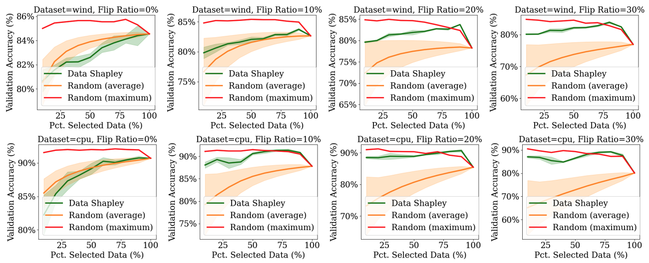
Figure 1: Validation accuracy curves as a function of the top $p\%$ most valuable data points added. The higher, the better. ‘Random (average)’ and ‘Random (maximum)’ mean sample different size-$k$ subsets uniformly at random and evaluate their average and maximum utility, respectively. Data Shapley’s error bar indicates the standard deviation across 5 independent runs where the randomness is from the permutation sampling of Data Shapley scores.

5.1 When MTM function is a good approximation?

The utility function $v$, being a set function determined by multiple factors such as the training set, learning algorithm, and performance metric, might be perceived as inherently complex. Therefore, it is interesting to understand the conditions under which $v$ can be well-approximated by some MTM functions. Specifically, we explore the connection between optimal fitting residuals and the consistency index of $v$, an intrinsic property of utility functions. We first define the concept of $\rho$-correlated dataset pairs.

Definition 7 ($\rho$-correlation (O’Donnell, 2014)).

We say a pair of random variables $S,S^{\prime}$ are $\rho$-correlated if they are sampled as follows: $S$ is sampled from $N$ uniformly at random ($S\sim\mathrm{Unif}(N)$), and for all $i\in S$, $i\notin S^{\prime}$ w.p. $(1-\rho)/2$, and for all $i\notin S$, $i\in S^{\prime}$ w.p. $(1-\rho)/2$. We use $\rho\text{-corr}(N)$ to denote the distribution of $\rho$-correlated subset pairs sampled from $N$.

Intuitively, commonly used learning algorithms are expected to demonstrate consistency in model behavior when trained on datasets that are similar or correlated. For example, if we have two datasets $S$ and $S^{\prime}$ that are closely related (as defined by the $\rho$-correlation), the performance of models trained on these datasets should not diverge significantly as the size of the training samples increases. This expectation leads to the anticipation of a high correlation between $v(S)$ and $v(S^{\prime})$ for utility functions that are related to test accuracy or loss. We refer to the correlation coefficient between $v(S)$ and $v(S^{\prime})$ for a pair of $\rho$-correlated $(S,S^{\prime})$ as the $\rho$-consistency index of a utility function, and we show that the high $\rho$-consistency index of a utility function, which suggests that minor perturbations in the training set do not lead to significant changes, serves as a positive signal for the existence of a reasonable MTM function approximation.

Theorem 8.

Let $\mathcal{M}$ denote the space of all MTM functions. For any utility functions $v$, we have

$$\min_{\widetilde{v}\in\mathcal{M}}\bar{\mathcal{R}}_{v}(\widetilde{v})\leq\frac{1}{1-\rho^{2}}\left(1-\texttt{cor}_{\rho}(v)\right)$$

where

is the correlation coefficient between $v(S)$ and $v(S^{\prime})$, which we referred to as the $\rho$-consistency index of $v$.

The result implies that when the values between $v(S)$ and $v(S^{\prime})$ have a stronger correlation when $S$ and $S^{\prime}$ are $\rho$-correlated, the utility function $v$ can be better approximated by MTM, which is intuitive as the mapping rules between $S$ and $v(S)$ is more tractable. The above theorem extends the classic result from harmonic analysis for the bound on the quality of the best linear approximation to a pseudo-boolean function in terms of its noise stability (O’Donnell, 2014). When we fix the monotonic function $f$ as the identity function $f(t)=t$, it reduces to Theorem 3.1 in Saunshi et al. (2022) after some rephrasing.

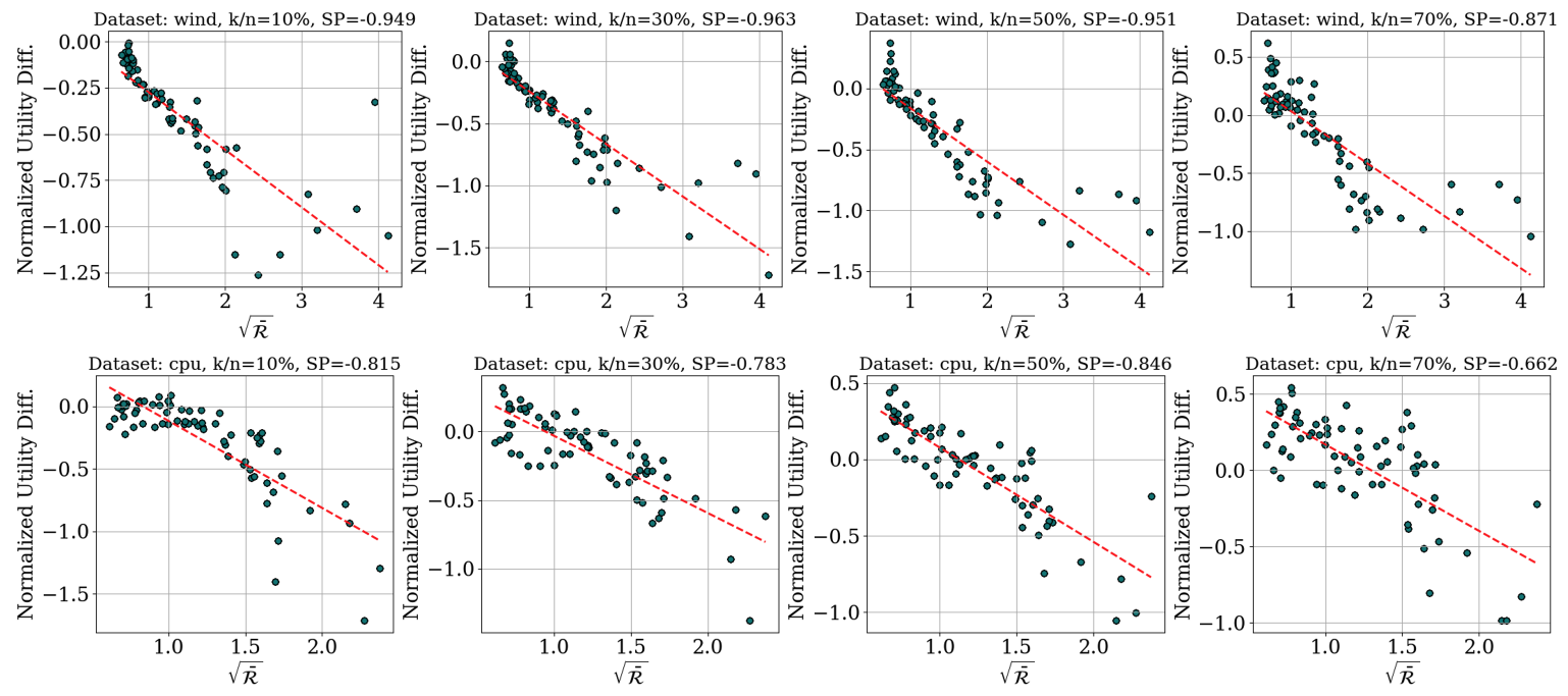
Figure 2: We investigate the correlation between data selection performance (measured by the normalized utility difference) and the normalized fitting residual of MTM function. For each dataset, we look at size-$k$ data selection performance with $k\in\{0.1n,0.3n,0.5n,0.7n\}$. Each point represents the results on a dataset (with different noise-flipping ratios).

6 Experiments

Our experiments aim to demonstrate the following assertions: (1) Data Shapley works well when the utility functions are being defined on heterogeneous datasets, (2) Data Shapley’s effectiveness is strongly correlated with the fitting quality of MTM functions to the utility functions, and (3) The utility functions’ approximability by MTM functions is further correlated with their $\rho$-consistency index (deferred to Appendix C.4). In this section, to estimate Data Shapley, we use the most widely used permutation sampling estimator (Mitchell et al., 2022), where for each experiment the sampling budget is as high as 40,000 to reduce the instability in Shapley value estimation. Following Ghorbani & Zou (2019); Kwon & Zou (2022), we use logistic regression as the learning algorithm here in the main paper. Additional results with neural networks and detailed experiment settings are deferred to Appendix C.

6.1 When does Data Shapley work well/bad for data selection?

To corroborate the reasonings in Section 3 and 4.1, we compare the efficacy of Data Shapley for data selection for datasets with different levels of varying data quality. To fairly evaluate the performance, we focus on Data Shapley’s relative performance compared with the random selection baseline. Specifically, for each cardinality $k$, we sample 50,000 subsets, evaluate their utility scores, and take the average. We also show the maximum utility score among all sampled subsets. We use 40,000 utility samples for approximating Data Shapley.

For each dataset, we create its noisy variants by randomly picking a certain proportion of the data points to flip their labels. Since mislabeled data usually negatively affect the model performance, its marginal contribution will likely be worse than any clean data points, mirroring the utility function structure described in Theorem 4. As depicted in Figure 1, we observe that for clean datasets (i.e., Flip Ratio=0%), the performance of subsets selected by Data Shapley marginally surpasses or worse than that of randomly chosen subsets, and significantly underperforms the subset with the maximum utility found by random selection. Conversely, in scenarios where datasets comprise data points of greater varied quality, the selection effectiveness of Data Shapley significantly improves. When the label-flipping ratio is high, Data Shapley closely matches or surpasses the highest utility found by random selection.

6.2 MTM Fitting Residual vs Data Selection Performance

We evaluate the effectiveness of the heuristic we proposed in Section 5 by assessing the correlation between MTM functions’ fitting residuals and Data Shapley’s performance in data selection.

Metric for Data Selection: normalized utility difference. Our metric for data selection performance is the normalized utility difference: the utility of the dataset selected by Data Shapley, $\widehat{S}_{\phi(v)}^{(k)}$, compared to the optimal dataset, $S_{*,v}^{(k)}$, normalized by the utility difference between the optimal dataset and random datasets, i.e., $\frac{v(\widehat{S}_{\phi(v)}^{(k)})-v(S_{*,v}^{(k)})}{v(S_{*,v}^{(k)})-\mathbb{E}_{S:|S|=k}[v(S)]}$. In practice, we approximate $v(S_{*,v}^{(k)})$ and $\mathbb{E}_{S:|S|=k}[v(S)]$ using the maximum and average utility of a batch of randomly sampled data subsets (same setting as in Section 6.1).

Neural network implementation of MTM function. We use a neural network-based parameterization for MTM. For a function $\widetilde{v}(S)=f(w_{0}+\sum_{i\in S}w_{i})$, we encode the dataset $S$ as a binary vector $x$, where $x_{i}=1$ if $i\in S$, and $x_{i}=0$ otherwise. The linear combination $w_{0}+\sum_{i=1}^{n}w_{i}x_{i}$ is implemented via a linear layer in the neural network. The monotonic function $f$ is implemented by a neural network with non-negative weight constraints. While such an approach may not guarantee finding the optimal $\widetilde{v}$, we empirically find that the fitting residual is fairly small (the mean squared error in most cases is $<10^{-4}$).

Results. For each dataset, we generate 200 noisy variants, where for each of the variants we randomly flip the label of a certain portion of data points where the noise rate is uniformly sampled between 0 and 50%. We then evaluate Data Shapley’s performance in size-$k$ data selection tasks across these datasets. Meanwhile, for each of the variants, a MTM function is trained to approximate its utility function and evaluate the fitting residual $\bar{\mathcal{R}}_{v}$. We reuse the 40,000 utility samples initially collected for Data Shapley estimation to train the MTM model. In the scatter plot in Figure 2, each dot corresponds to one of the dataset’s variants. We present the result for data selection ratios of $k/n\in\{10\%,30\%,50\%,70\%\}$. We can see a clear correlation between Data Shapley’s performance on size-$k$ data selection task and the normalized fitting residual of the MTM function. Notably, a lower $\bar{\mathcal{R}}_{v}$ consistently corresponds with Data Shapley’s capability to identify datasets of higher utility. When $\bar{\mathcal{R}}_{v}$ is large, data selection performance indeed tends to exhibit significant variance, making its predictability challenging. This is expected as being a MTM function is only a sufficient condition for being Shapley-effective.

7 Conclusion & Limitations

This work advances the understanding of the application of Data Shapley for data selection tasks. We show that Data Shapley’s performance can be no better than basic random selection in general settings, and we discuss the conditions under which Data Shapley excels.

Limitations. In our experiment, we demonstrate that our heuristic is highly effective when comparing Data Shapley’s effectiveness among utility functions for datasets from the same domain but of different qualities. However, its applicability is less certain when comparing utility functions for datasets from different domains. This is expected as the huge differences in the function nature make their approximability or learnability not directly comparable. Despite this limitation, the heuristic remains valuable in many practical scenarios where we are dealing with datasets from the same domain but with differing qualities. In such cases, the heuristic can be used in predicting the usefulness of Data Shapley for data selection within each source.

Future works. Building on the insights from this study, future research could explore the sufficient and necessary conditions for which Data Shapley is optimal for data selection. Additionally, a deeper exploration into the ethical implications and fairness aspects of the downstream applications of Data Shapley could be an interesting future work.

Appendix A Extended Related Works

A.1 Data Shapley and Friends

Data Shapley is one of the first principled approaches to data valuation being proposed (Ghorbani & Zou, 2019; Jia et al., 2019b). Data Shapley is based on the Shapley value, a famous solution concept from game theory literature which is almost always being justified as the unique value notion satisfying the following four axioms:

1. Null player: if $v(S\cup\{z_{i}\})=v(S)$ for all $S\subseteq D\setminus\{z_{i}\}$, then $\phi_{z_{i}}(v)=0$.

2. Symmetry: if $v(S\cup\{z_{i}\})=v(S\cup\{z_{j}\})$ for all $S\subseteq D\setminus\{z_{i},z_{j}\}$, then $\phi_{z_{i}}(v)=\phi_{z_{j}}(v)$.

3. Linearity: For utility functions $v_{1},v_{2}$ and any $\alpha_{1},\alpha_{2}\in\mathbb{R}$, $\phi_{z_{i}}(\alpha_{1}v_{1}+\alpha_{2}v_{2})=\alpha_{1}\phi_{z_{i}}(v_{1})+\alpha_{2}\phi_{z_{i}}(v_{2})$.

4. Efficiency: for every $v,\sum_{z_{i}\in D}\phi_{z_{i}}(v)=v(D)$.

Since its introduction, Data Shapley has rapidly gained popularity as a principled solution for data valuation. However, as argued in (Kwon & Zou, 2022), the efficiency axiom is not necessary for the machine learning context, and the framework of semivalue is obtained by relaxing the efficiency axiom. Moreover, (Lin et al., 2022) provide an alternative justification for semivalue based on causal inference and randomized experiments. Based on the framework of semivalue, (Kwon & Zou, 2022) propose Beta Shapley, which is a collection of semivalues that enjoy certain mathematical convenience. (Wang & Jia, 2023a) propose Data Banzhaf, and show that the Banzhaf value, another famous solution concept from cooperative game theory, is the most reproducible against arbitrary perturbation to the submodels. Furthermore, the leave-one-out error is also a semivalue, where the influence function (Koh & Liang, 2017) is generally considered as its approximation. Another line of works focuses on improving the computational efficiency of Data Shapley by considering KNN as the surrogate learning algorithm for the original, potentially complicated deep learning models (Jia et al., 2019a; Wang et al., 2023, 2024). (Ghorbani et al., 2020; Kwon et al., 2021) consider Distributional Shapley, a generalization of Data Shapley to data distribution.

A.2 Alternative Data Valuation Methods

There have also been approaches for data valuation that do not belong to the aforementioned types. For a detailed survey, we direct readers to (Sim et al., 2022). Notably, several studies have focused on tracking the impact of individual training examples on test loss throughout the training process (Pruthi et al., 2020; Hammoudeh & Lowd, 2021; Paul et al., 2021; Yeh et al., 2022; Das et al., 2022; Guu et al., 2023). Another avenue of research employs the representer theorem to decompose neural network predictions into linear combinations of training data activations (Yeh & Lien, 2009; Sui et al., 2021). However, (Søgaard et al., 2021) revealed the empirical instability of techniques such as TracIn (Pruthi et al., 2020) and the Representer Point method (Yeh et al., 2018).

Further, (Sim et al., 2020) introduced a valuation metric based on the reduction in model parameter uncertainty provided by the data. Several training-free and task-agnostic data valuation methods have also been proposed. For instance, (Xu et al., 2021) proposed a diversity measure known as robust volume (RV) for appraising data sources. (Tay et al., 2022) devised a valuation method leveraging the maximum mean discrepancy (MMD) between the data source and the actual data distribution. (Nohyun et al., 2022) introduced a complexity-gap score for evaluating data value without training, specifically in the context of overparameterized neural networks. (Wu et al., 2022) applied a domain-aware generalization bound based on neural tangent kernel (NTK) theory for data valuation. (Amiri et al., 2022) assessed data value by measuring statistical differences between the source data and a baseline dataset. (Just et al., 2022) utilized a specialized Wasserstein distance between training and validation sets as the utility function, alongside an efficient approximation of the LOO error. Lastly, (Kwon & Zou, 2023) utilized random forests as proxy models to propose an efficient, validation-free data valuation algorithm.

Appendix B Deferred Proofs

Theorem 9 (Restate of Theorem 2).

Given any two subsets of training data $S_{1},S_{2}\subseteq N$ such that $S_{1}\neq S_{2}$ and $S_{i}\neq\varnothing$ and $S_{i}\neq N$ for $i\in\{1,2\}$, the null and alternative hypothesis is formed as follows:

$$H_{(0)}:v(S_{1})\geq v(S_{2})$$ (3)

$$H_{(a)}:v(S_{1})<v(S_{2})$$

Any Shapley value-based hypothesis test $\mathbf{h}$ for the above problem is constrained to:

$$\textbf{TrueNeg}(\mathbf{h})+\textbf{TruePos}(\mathbf{h})\leq 1$$

Proof.

This result immediately follows from Theorem 3, since no matter what value score $s\in\mathbb{R}^{n}$ is available to $\mathbf{h}$, there always exists $v\in\mathcal{F}^{(0)}_{S_{1},S_{2}}$ and $v^{\prime}\in\mathcal{F}^{(a)}_{S_{1},S_{2}}$ that yields the same Shapley vector $s=\phi(v)=\phi(v^{\prime})$, where $\mathbf{h}(s)$ cannot distinguish between $v$ and $v^{\prime}$ based on $s$. ∎

Theorem 10 (Restate of Theorem 3).

Given any score vector $s\in\mathbb{R}^{n}$ and any two subsets of training data $S_{1},S_{2}\subseteq N$ such that $S_{1}\neq S_{2}$ and $S_{i}\neq\varnothing$ and $S_{i}\neq N$ for $i\in\{1,2\}$, there exists two utility functions $v$ and $v^{\prime}$ s.t. $v\in\mathcal{F}^{(0)}_{S_{1},S_{2}}$ and $v^{\prime}\in\mathcal{F}^{(a)}_{S_{1},S_{2}}$, and both yield the same Shapley vector: $s=\phi(v)=\phi(v^{\prime})$.

Proof.

If we view the computation of the Shapley value $\phi$ as a function from the utility function $v$, and if we view the utility function as a size-$(2^{n}-1)$ vector , then the Shapley value can be viewed as a linear mapping from $\mathbb{R}^{2^{n}-1}$ to $\mathbb{R}^{n}$. That is, $\phi=Av$ for some matrix $A\in\mathbb{R}^{n\times(2^{n}-1)}$. This can be easily inferred from the Shapley value’s formula in Definition 1. For a given data subset $T\subseteq N$, we define a simple game $\bar{u}_{T}$ with the utility function as follows:

$$\bar{u}_{T}(S)=\begin{cases}1&|S\land T|=1\\ 0&\text{Otherwise}\end{cases}$$

Such a game is referred as commander’s game in the literature (Yokote et al., 2016), where one can show that $\phi(\bar{u}_{T})=A\bar{u}_{T}=\mathbf{0}$, and the set of $\{\bar{u}_{T}:T\subseteq N,|T|\geq 1\}$ forms a basis for $\mathbb{R}^{2^{n}-1}$. By (Yokote et al., 2016), for any utility function $v$ with the Shapley value $s=\phi(v)$, we can decompose it as

$$v(S)=\sum_{i\in S}s_{i}+\sum_{T\subseteq N,|T|\geq 2}\alpha_{T}\bar{u}_{T}(S)$$

Now, as long as we can show that there always exists $\{\alpha_{T}\}_{T\subseteq N,|T|\geq 2}$ that can form a utility function $v$ s.t. $v(S_{1})\geq v(S_{2})$, we can construct $v\in\mathcal{F}^{(0)}_{S_{1},S_{2}}$ required by the theorem statement.

$$v(S_{1})-v(S_{2}) =\left(\sum_{i\in S_{1}}s_{i}+\sum_{T\subseteq N,|T|\geq 2}\alpha_{T}\bar{u}_{T}(S_{1})\right)-\left(\sum_{i\in S_{2}}s_{i}+\sum_{T\subseteq N,|T|\geq 2}\alpha_{T}\bar{u}_{T}(S_{2})\right)$$

$$=\sum_{i\in S_{1}\setminus S_{2}}s_{i}-\sum_{i\in S_{2}\setminus S_{1}}s_{i}+\sum_{T\subseteq N,|T|\geq 2}\alpha_{T}\left(\bar{u}_{T}(S_{1})-\bar{u}_{T}(S_{2})\right)$$

Since any of $\alpha_{T}$ can be set to be arbitrarily large to force $v(S_{1})-v(S_{2})\geq 0$, all we need is having $\{T:|T|\geq 2,|T\land S_{1}|=1,|T\land S_{2}|\neq 1\}$ is non-empty so that there exists at least one of $T$ s.t. $\bar{u}_{T}(S_{1})-\bar{u}_{T}(S_{2})>0$. This is clearly true when $S_{1}\neq S_{2}$ and $S_{i}\neq\varnothing$ and $S_{i}\neq N$ for $i\in\{1,2\}$.

The construction of $v^{\prime}$ can be done similarly. ∎

Theorem 11 (Restate of Theorem 6).

For any utility functions $v$ that is monotonically transformed modular, Data Shapley is optimal for size-$k$ data selection tasks for any $k=1,\ldots,n-1$.

Proof.

Without loss of generality, let $w_{1}\geq\ldots\geq w_{n}$. Since $f$ is a monotonic function, it is clear that the optimal size-$k$ subset $S_{*,v}^{(k)}=\{1,\ldots,k\}$. We now show that for such a utility function $v$, $\phi_{i}(v)\geq\phi_{j}(v)$ for any $i\geq j$. This immediately follows from the fact that for any $S\subseteq N\setminus\{i,j\}$ we have $v(S\cup i)=f(w_{0}+\sum_{\ell\in S}w_{\ell}+w_{i})\geq f(w_{0}+\sum_{\ell\in S}w_{\ell}+w_{j})=v(S\cup j)$ as $w_{i}\geq w_{j}$ in the assumption. Since $\phi_{i}-\phi_{j}$ can be written as a positively weighted sum of $v(S\cup i)-v(S\cup j)$ across $S\subseteq N\setminus\{i,j\}$, we have $\phi_{1}\geq\phi_{2}\geq\ldots\geq\phi_{n}$ and $S_{*,v}^{(k)}$ consists of data points with top-$k$ Data Shapley scores.

∎

Theorem 12 (Restate of Theorem 8).

Denote the subclass of monotonically transformed modular (MTM) function defined on $N$ as $\mathcal{M}$, i.e., $\mathcal{M}:=\{v:\exists\text{monotonic}~{}f,\exists w\in\mathbb{R}^{n}~{}\text{s.t.}~{}\forall S\subseteq N:f(w_{0}+\sum_{i\in S}w_{i})=v(S)\}$. For all $\rho\in[0,1)$ we have

$$\min_{\widetilde{v}\in\mathcal{M}}\bar{\mathcal{R}}_{v}(\widetilde{v})\leq\frac{1}{1-\rho^{2}}\left(1-\texttt{cor}_{\rho}(v)\right)$$

where

$$\texttt{cor}_{\rho}(v):=\frac{\underset{(S,S^{\prime})\sim\rho\text{-corr}(N)}{\mathbb{E}}\left[v(S)v(S^{\prime})\right]-\mathbb{E}_{S\sim\mathrm{Unif}(N)}\left[v(S)\right]^{2}}{\mathrm{Var}_{S\sim\mathrm{Unif}(N)}(v(S))}$$

is the correlation coefficient between $v(S)$ and $v(S^{\prime})$, which we referred to as the $\rho$-consistency index of $v$.

Proof.

Denote the monotonic function class $\mathcal{F}_{\gamma}=\{f:\frac{\max_{t}f^{\prime}(t)}{\min_{t}f^{\prime}(t)}=\gamma,\min_{t}f^{\prime}(t)>0\}$. Denote the subclass of $\mathcal{M}$ as $\mathcal{M}_{\gamma}=\{v:v(S)=f(w_{0}+\sum_{i\in S}w_{i}),f\in\mathcal{F}_{\gamma}\}$.

First, the space of function class $\mathcal{M}_{\gamma}$ will be remain the same if we further restrict that $f(0)=0$, as for any $v(S)=f(w_{0}+\sum_{i\in S}w_{i})$ with $f(0)\neq 0$, it can be equivalently expressed as $v(S)=f_{0}\left(w_{0}-f^{-1}(0)+\sum_{i\in S}w_{i}\right)$ with $f_{0}(t)=f(t+f^{-1}(0))$. Note that $f^{-1}(0)$ always exists due to the condition that $f^{\prime}(t)\geq L$ for some constant $L>0$.

Now, we fix a monotonic function $f\in\mathcal{F}_{\gamma}$ s.t. $f(0)=0$, and we denote $U:=\max_{t}f^{\prime}(t),L:=\min_{t}f^{\prime}(t)$, i.e., $\gamma=U/L$.

Denote $g(S)=f^{-1}(v(S))$. From Theorem 3.1 in Saunshi et al. (2022), we know that

$$\min_{w}\mathbb{E}_{S}\left[(g(S)-w_{0}-\sum_{i\in S}w_{i})^{2}\right]\leq\frac{1}{1-\rho^{2}}\left(\mathbb{E}_{S}\left[g(S)^{2}\right]-\underset{(S,S^{\prime})\sim\rho\text{-corr}(N)}{\mathbb{E}}\left[g(S)g(S^{\prime})\right]\right)$$

Denote $w^{*}=\operatorname*{\arg\!\min}_{w}\mathbb{E}_{S}\left[(g(S)-w_{0}-\sum_{i\in S}w_{i})^{2}\right]$.

Since $f^{\prime}(t)\in[L,U]$, we have

$$\left|v(S)-f\left(w_{0}+\sum_{i\in S}w_{i}\right)\right| =\left|f(f^{-1}(v(S)))-f\left(w_{0}+\sum_{i\in S}w_{i}\right)\right|$$

$$\leq U\left|f^{-1}(v(S))-w_{0}-\sum_{i\in S}w_{i}\right|$$

and since the derivative of inverse function $(f^{-1})^{\prime}\in[1/U,1/L]$, we have

$$g(S)=f^{-1}(v(S))=f^{-1}(v(S))-f^{-1}(0)\in\left[\frac{v(S)}{U},\frac{v(S)}{L}\right]$$

Hence, we know that

$$\mathbb{E}_{S}\left[\left(v(S)-f\left(w_{0}^{*}+\sum_{i\in S}w_{i}^{*}\right)\right)^{2}\right] \leq U^{2}\mathbb{E}_{S}\left[\left(g(S)-w_{0}^{*}-\sum_{i\in S}w_{i}^{*}\right)^{2}\right]$$

$$\leq\frac{U^{2}}{1-\rho^{2}}\left(\mathbb{E}_{S}\left[g(S)^{2}\right]-\underset{(S,S^{\prime})\sim\rho\text{-corr}(N)}{\mathbb{E}}\left[g(S)g(S^{\prime})\right]\right)$$

$$\leq\frac{U^{2}}{1-\rho^{2}}\left(\frac{1}{L^{2}}\mathbb{E}_{S}\left[v(S)^{2}\right]-\frac{1}{U^{2}}\underset{(S,S^{\prime})\sim\rho\text{-corr}(N)}{\mathbb{E}}\left[v(S)v(S^{\prime})\right]\right)$$

$$=\frac{1}{1-\rho^{2}}\left(\gamma^{2}\mathbb{E}_{S}\left[v(S)^{2}\right]-\underset{(S,S^{\prime})\sim\rho\text{-corr}(N)}{\mathbb{E}}\left[v(S)v(S^{\prime})\right]\right)$$

Therefore, we have

$$\min_{\widetilde{v}\in\mathcal{M}_{\gamma}}\mathbb{E}_{S}\left[\left(v(S)-\widetilde{v}(S)\right)^{2}\right] \leq\min_{w}\mathbb{E}_{S}\left[\left(v(S)-f\left(w_{0}+\sum_{i\in S}w_{i}\right)\right)^{2}\right]$$

$$\leq\frac{1}{1-\rho^{2}}\left(\gamma^{2}\mathbb{E}_{S}\left[v(S)^{2}\right]-\underset{(S,S^{\prime})\sim\rho\text{-corr}(N)}{\mathbb{E}}\left[v(S)v(S^{\prime})\right]\right)$$

$$=\frac{1}{1-\rho^{2}}\left(\gamma^{2}\left(\mathrm{Var}_{S}\left(v(S)\right)+\mathbb{E}_{S}\left[v(S)\right]^{2}\right)-\underset{(S,S^{\prime})\sim\rho\text{-corr}(N)}{\mathbb{E}}\left[v(S)v(S^{\prime})\right]\right)$$

Note that $\gamma\geq 1$. Clearly, the upper bound is minimized when $\gamma=1$. Hence, we have

$$\min_{\widetilde{v}\in\mathcal{M}_{\gamma}}\mathbb{E}_{S}\left[\left(v(S)-\widetilde{v}(S)\right)^{2}\right] \leq\frac{1}{1-\rho^{2}}\left(\mathrm{Var}_{S}\left(v(S)\right)+\mathbb{E}_{S}\left[v(S)\right]^{2}-\underset{(S,S^{\prime})\sim\rho\text{-corr}(N)}{\mathbb{E}}\left[v(S)v(S^{\prime})\right]\right)$$

Dividing both sides by $\mathrm{Var}_{S}(v(S))$ gives the inequality in the statement. ∎

Theorem 13 (Restate of Theorem 4).

Suppose that the dataset $N$ can be divided into $N=S_{\text{bad}}\cup S_{\text{clean}}$ where $S_{\text{bad}}\cap S_{\text{clean}}=\varnothing$, $|S_{\text{clean}}|=k$. If the utility function $v$ fulfills the condition: $\forall j\in S_{\text{clean}},\forall i\in S_{\text{bad}},\forall S\subseteq N\setminus\{i,j\},~{}v(S\cup i)\leq v(S\cup j)$ then Data Shapley is optimal for size-$k$ data selection problem.

Proof.

We show the following two statements: (1) $S_{\text{clean}}$ consists of the data points of top-$k$ Shapley values among $N$ and (2) $v(S_{\text{clean}})=\operatorname*{\arg\!\max}_{S:S\subseteq N,|S|=k}v(S)$.

For (1), $S_{\text{clean}}$ consists of the data points of top-$k$ Shapley values among $N$ since for any $j\in S_{\text{clean}}$ and $i\in S_{\text{bad}}$, we have $\phi_{j}\geq\phi_{i}$ which immediately follows from the condition of $\forall S\subseteq N\setminus\{i,j\},~{}v(S\cup i)\leq v(S\cup j)$. For (2), we prove the following argument for any $\ell\geq 0$ with induction: for any $S\subseteq N$ of size $k$ s.t. $|S\setminus S_{\text{clean}}|=|S_{\text{clean}}\setminus S|=\ell$, we have $v(S)\leq v(S_{\text{clean}})$. The base case when $\ell=0$ trivially holds. Now, suppose that the statement holds true for all $\ell\leq L-1$. Now, consider an $S$ where $|S\setminus S_{\text{clean}}|=L$. Consider an alternative $S^{\prime}\subseteq N$ and $|S^{\prime}|=k$ where $S^{\prime}\setminus S=\{j\}$ for some $j\in S_{\text{clean}}$ and $S\setminus S^{\prime}=\{i\}$ for some $i\in S_{\text{bad}}$. That is, $S^{\prime}$ is constructed by removing an $i\in S_{\text{bad}}$ by an $j\in S_{\text{clean}}$. Let $S^{\prime\prime}:=S\cup S^{\prime}$. We have $v(S^{\prime})=v(S^{\prime\prime}\cup j)\geq v(S^{\prime\prime}\cup i)=v(S)$. Moreover, since $|S^{\prime}\setminus S_{\text{clean}}|=L=1$, by induction hypothesis we have $v(S^{\prime})\leq v(S_{\text{clean}})$, which implies that $v(S)\leq v(S_{\text{clean}})$. ∎

B.1 Extension of Theorem 3 to Semivalue

Semivalue (Dubey et al., 1981) is originally studied in cooperative game theory. It has recently been proposed as a unified framework for data value notions (Kwon & Zou, 2022; Lin et al., 2022) which comprises many existing data value notions such as LOO (Koh & Liang, 2017), Data Shapley (Ghorbani & Zou, 2019), Beta Shapley (Kwon & Zou, 2022), and Data Banzhaf (Wang & Jia, 2023a). The popularity of semivalues is attributable to the fact that they are the collection of all possible data value notions that satisfy three important axioms: dummy player, symmetry, and linearity. The specific definition of the three axioms can be found in Appendix A.

Definition 14 (Semivalues).

We say a data value notion is a semivalue if and only if it satisfies the linearity, dummy player, and symmetry axioms.

The following theorem shows that every semivalue of a data point $i$ can be expressed as a weighted average of marginal contributions $v(S\cup i)-v(S)$ across different subsets $S\subseteq N\setminus i$.

Theorem 15 (Representation of Semivalue (Dubey et al., 1981)).

A value function $\phi$ is a semivalue, if and only if, there exists a set of weights $\{\alpha^{(n)}_{k},k=1,\ldots,n\}$ such that $\sum_{k=1}^{n}{n-1\choose k-1}\alpha^{(n)}_{k}=1$ and the value function $\phi$ can be expressed as follows:

$$\phi_{i}\left(v\right):=\frac{1}{n}\sum_{k=1}^{n}\alpha^{(n)}_{k}\sum_{\begin{subarray}{c}S\subseteq N\setminus i,\\ |S|=k-1\end{subarray}}\left(v(S\cup i)-v(S)\right)$$

For example, when $\alpha^{(n)}_{k}=\frac{1}{n}{n-1\choose k-1}^{-1}$, it reduces to the Shapley value. When $\alpha^{(n)}_{k}=\frac{1}{2^{n-1}}$, it reduces to the Banzhaf value. When $\alpha^{(n)}_{k}=\mathbbm{1}[k=n]$, it reduces to the LOO error.

Definition 16 (inverse Pascal triangle condition (Dragan, 2002)).

We say a semivalue $\phi$ with weights coefficients $\alpha^{(n)}_{k}$ satisfies the “inverse Pascal triangle condition” if

$$\forall t=1,2,\ldots,\forall k\in\{1,2,\cdots,t-1\}:\alpha_{k}^{(t-1)}=\alpha_{k}^{(t)}+\alpha_{k+1}^{(t)}$$

We can easily verify that this condition is satisfied for all of LOO, the Shapley value, and the Banzhaf value.

Theorem 17.

Given a semivalue $\phi$ with weights coefficients $\alpha^{(n)}_{k}$, if it satisfies the “inverse Pascal triangle condition”, then for any score vector $s\in\mathbb{R}^{n}$ and any two subsets of training data $S_{1},S_{2}\subseteq N$ such that $S_{1}\neq S_{2}$ and $S_{i}\neq\varnothing$ and $S_{i}\neq N$ for $i\in\{1,2\}$, there exists two utility functions $v$ and $v^{\prime}$ s.t. $v\in\mathcal{F}^{(0)}_{S_{1},S_{2}}$ and $v^{\prime}\in\mathcal{F}^{(a)}_{S_{1},S_{2}}$, and both yield the same semivalue vector: $s=\phi(v)=\phi(v^{\prime})$.

Proof.

Similar to the proof for Theorem 3, we exploit the null space of semivalue.

For a given data subset $T\subseteq N$, we define a utility function $w_{T}$ as follows:

$$w_{T}(S)=\left\{\begin{aligned} &\sum_{c=0}^{|S|-|T|}{(-1)^{c}\left(\begin{matrix}|S|-|T|\\ c\end{matrix}\right)}/\alpha_{c+|T|}^{c+|T|}&S\supsetneq T\\ &1/\alpha_{|T|}^{|T|}&S=T\\ &0&S\subsetneq T\end{aligned}\right.$$

By (Dragan, 2002), for any semivalue $\phi$ that satisfies the inverse Pascal triangle condition, $\{w_{T}:T\subseteq N,T\neq\emptyset\}$ is a basis for the space of utility functions, and for any utility function $v$ with the semivalue $s=\phi(v)$, we can decompose it as

$$v(S)=\sum_{|T|\leq n-2}\beta_{T}w_{T}(S)+\beta_{N}\left(w_{N}(S)+\sum_{i\in N}w_{N\setminus i}(S)\right)-\sum_{i\in N}s_{i}w_{N\setminus i}(S)$$

Moreover, by (Dragan, 2002), the set $\{w_{T}(S):1\leq|T|\leq n-2\}\cup\{w_{N}+\sum_{i\in N}w_{N\setminus i}\}$ is a basis for the null space of semivalue $\phi$, i.e., $\phi(w)=0$ for all utility functions $w$ from this set.

Now, as long as we can show that there always exists $\{\beta_{T}\}_{T\subseteq N}$ that can form a utility function $v$ s.t. $v(S_{1})\geq v(S_{2})$, we can construct $v\in\mathcal{F}^{(0)}_{S_{1},S_{2}}$ required by the theorem statement.

$$v(S_{1})-v(S_{2})= \sum_{|T|\leq|N|-2}\beta_{T}(w_{T}(S_{1})-w_{T}(S_{2}))$$

$$+\beta_{N}\left(w_{N}(S_{1})-w_{N}(S_{2})+\sum_{i\in N}[w_{N\setminus i}(S_{1})-w_{N\setminus i}(S_{2})]\right)$$

$$-\sum_{i\in N}s_{i}\cdot(w_{N\setminus i}(S_{1})-w_{N\setminus i}(S_{2}))$$

Since $\beta_{T}(v)$ can set to be arbitrarily large to make $v(S_{1})-v(S_{2})\geq 0$, all we need is having at least one $w_{T}(S_{1})\neq w_{T}(S_{2})$, which is clearly true when $S_{1}\neq S_{2}$ and none of $S_{1}$ or $S_{2}$ equals $N$ or $\varnothing$ .

The construction of $v^{\prime}$ can be done similarly using previous techniques.

∎

Appendix C Additional Settings & Experiments

C.1 Datasets & Architectures

Datasets.

An overview of the dataset information we used in Section 6 can be found in Table 2. These are commonly used datasets in the existing literature in data valuation (Ghorbani & Zou, 2019; Kwon & Zou, 2022; Jia et al., 2019b; Wang & Jia, 2023a; Kwon & Zou, 2023; Wang et al., 2024). Following Kwon & Zou (2022), for the datasets that have multi-class, we binarize the label by considering $\mathbbm{1}[y=1]$. Given the large amount of model retraining required in our experiment, for each of the dataset we take a size-200 subset as the training set, and a size-2000 subset as the validation set. This is the same as prior studies in Data Shapley (Kwon & Zou, 2022; Wang & Jia, 2023a).

Dataset	Source
Wind	https://www.openml.org/d/847
CPU	https://www.openml.org/d/761
Fraud	(Dal Pozzolo et al., 2015)
2DPlanes	https://www.openml.org/d/727
Vehicle	(Duarte & Hu, 2004)
Apsfail	https://www.openml.org/d/41138
Pol	https://www.openml.org/d/722

Table 2: A summary of datasets used in Section 6’s experiments.

Architectures.

In the experiments in the main paper, we use logistic regression as the learning algorithm. Here in Appendix, we also show the results when using a two-layer MLP model as the learning algorithm, where there are 100 neurons in the hidden layer, activation function ReLU, batch size $128$, (initial) learning rate $10^{-2}$ and Adam optimizer for training.

Architecture for training MTM function.

In Section 6.2 and Appendix C.4, we use a neural network-based parameterization for MTM. For a function $\widetilde{v}(S)=f(w_{0}+\sum_{i\in S}w_{i})$, we encode the dataset $S$ as a binary vector $x$, where $x_{i}=1$ if $i\in S$, and $x_{i}=0$ otherwise. The linear combination $w_{0}+\sum_{i=1}^{n}w_{i}x_{i}$ is implemented via a linear layer in the neural network. The monotonic function $f$ is implemented by a neural network with non-negative weight constraints. While such an approach may not guarantee finding the optimal $\widetilde{v}$, we find that the fitting residual is fairly small (the mean squared error in most cases is $<10^{-4}$). We use an MLP with 2 hidden layers to implement the monotonic function $f$, where each layer has 100 neurons. We add an attention layer between the first and the second hidden layer. We reuse the 40,000 utility samples collected from Shapley value estimation for the training and testing of MTM, where we split the utility samples into 32,000 for training and 8,000 for evaluation. We use batch size $32$, (initial) learning rate $10^{-3}$, and Adam optimizer for training 10 epochs.

C.2 Additional Experiments for Section 6.1

In Figure 3, we show the data selection results for additional datasets when using logistic regression classifiers. In Figure 4, we show the data selection results when using MLP classifiers. We note that in this case, because there is randomness during model training, the maximum utility found by random selection baseline can be higher than other approaches when trained on full datasets. The results are similar to what is observed from the maintext: for clean datasets, Data Shapley’s performance is much worse than that of their noisy variants, which corroborates the insights that without additional constraints on the underlying utility function’s characteristics (such as the quality of particular data points), the performance of Data Shapley can be no better than random guessing.

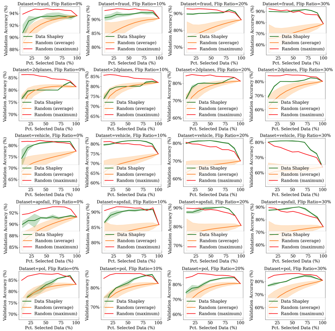
Figure 3: Additional results when using logistic regression classifiers. Validation accuracy curves as a function of the most valuable data points added. The higher, the better. ‘Random (average)’ and ‘Random (maximum)’ means sample different size-$k$ subsets uniformly and random and evaluate their average and maximum utility, respectively. Data Shapley’s error bar indicates the standard deviation across 5 independent runs where the randomness is from the permutation sampling of Data Shapley scores.

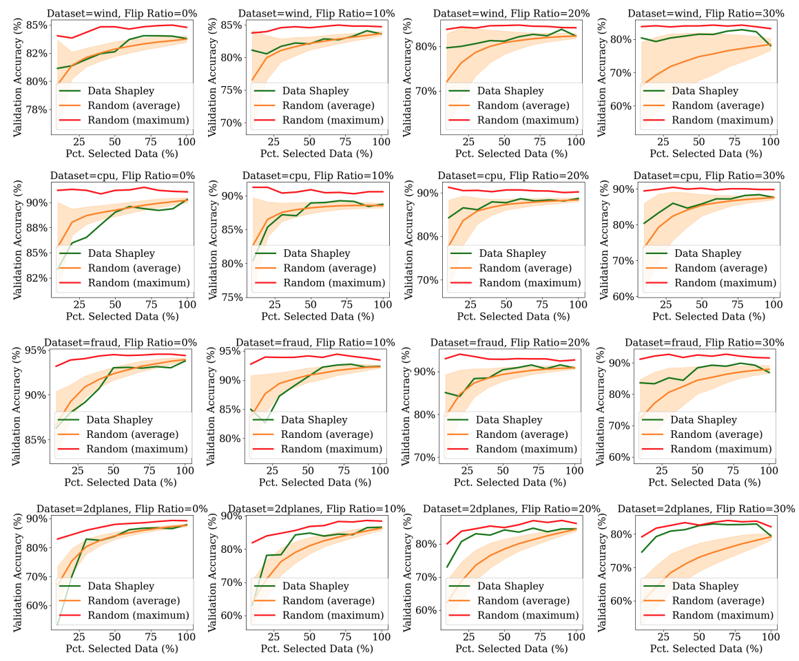
Figure 4: Additional results when using MLP classifiers. The figure shows the validation accuracy curves as a function of the most valuable data points added. The higher, the better. ‘Random (average)’ and ‘Random (maximum)’ means sample different size-$k$ subsets uniformly and random and evaluate their average and maximum utility, respectively. Data Shapley’s error bar indicates the standard deviation across 5 independent runs where the randomness is from the permutation sampling of Data Shapley scores.

C.3 Additional Experiments for Section 6.2

In Figure 5, we show the results for comparing Data Shapley’s data selection performance and $\bar{\mathcal{R}}_{v}$ on additional datasets, and in Figure 6 we show additional results on MLP classifiers. Similar to the results in the maintext, the fitting residual of MTM function and Data Shapley’s performance exhibit a strong correlation, which further validates the effectiveness of the heuristic proposed in Section 5.

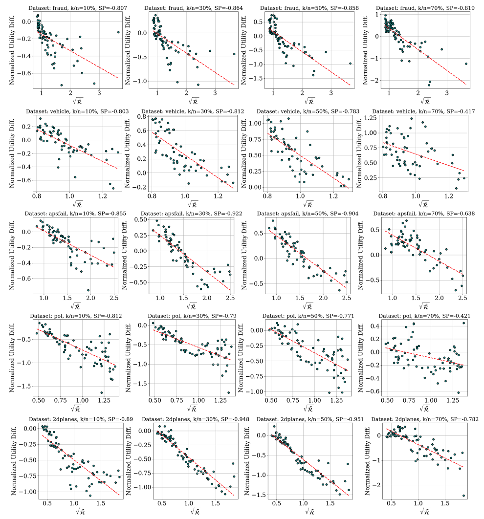
Figure 5: Results on additional datasets for the correlation between $\bar{\mathcal{R}}_{v}$ and data selection performance. We investigate the correlation between data selection performance and the normalized fitting residual of MTM function. For each dataset, we look at size-$k$ data selection performance with $k\in\{0.1n,0.3n,0.5n,0.7n\}$. Each point represents the results on a dataset (with different noise-flipping ratios).

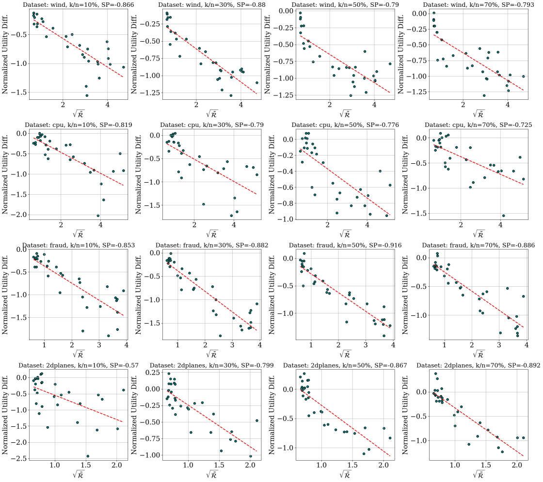
Figure 6: Results for the correlation between $\bar{\mathcal{R}}_{v}$ and data selection performance when using MLP classifier. We investigate the correlation between data selection performance and the normalized fitting residual of MTM function. For each dataset, we look at size-$k$ data selection performance with $k\in\{0.1n,0.3n,0.5n,0.7n\}$. Each point represents the results on a dataset (with different noise-flipping ratios).

C.4 MTM Fitting Residual vs $\rho$-Consistency Index

In this experiment, we investigate the correlation between the fitting residual of MTM function and $\rho$-consistency index $\texttt{cor}_{\rho}(v)$ defined in Theorem 8. The setting in this experiment is the same as the one in Section 6.2, and we additionally compute the $\rho$-consistency index for each noisy variant. Following the theorem’s guidance, our focus is on scenarios with relatively low noise rates ($\rho\in\{0,0.1,0.2,0.3\}$). For each specified value of $\rho$, we generate 5000 pairs of $\rho$-correlated datasets $S,S^{\prime}$ and estimate $\rho$-consistency index $\texttt{cor}_{\rho}(v)$.

Figure 7 and 8 show the results on logistic and MLP classifier, respectively. As we can see, there is a strong correlation between $\rho$-consistency index and the fitting residual $\bar{\mathcal{R}}_{v}(v)$. This observation lends empirical support to the theoretical assertions made in Theorem 8, suggesting that $\rho$-consistency index is indeed a significant factor in determining the fitting quality of MTM functions to utility functions. Since MTM’s fitting residual is correlated to the Data Shapley’s data selection performance as we have shown earlier, $\texttt{cor}_{\rho}(v)$ is also highly correlated with Data Shapley’s data selection performance, as validated in Figure 9 and 10. This is because for noisy datasets, since two correlated subsets are likely to both contain similar amounts of bad data, their utilities have a stronger correlation compared with clean datasets where data points are of similar quality.

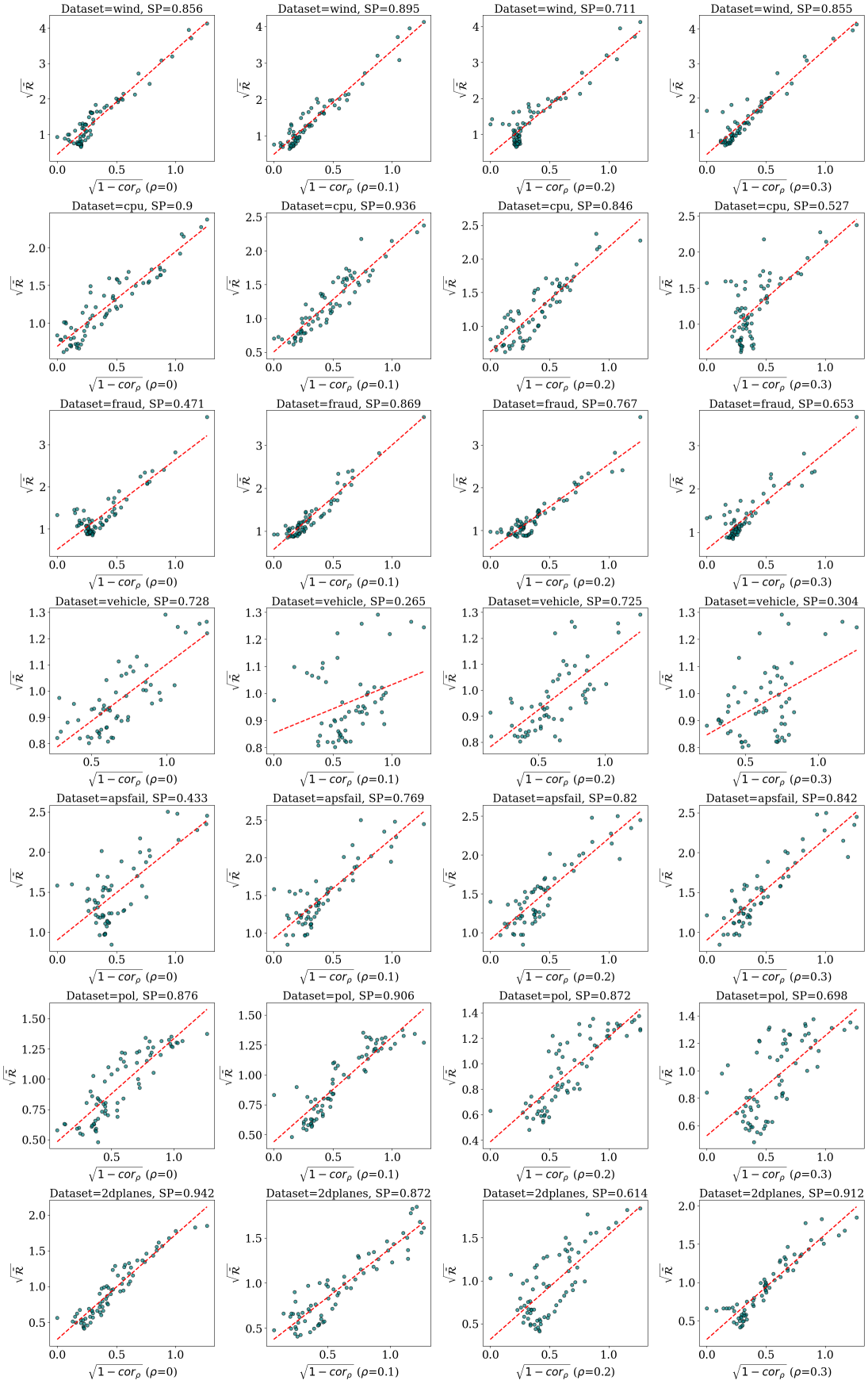
Figure 7: We investigate the correlation between the normalized fitting residual of MTM and the $\rho$-consistency index of the utility functions. The results for other values of $\rho$s are deferred to Appendix C. We vary different $\rho\in\{0,0.1,0.2,0.3\}$ and estimate the $\rho$-consistency index.

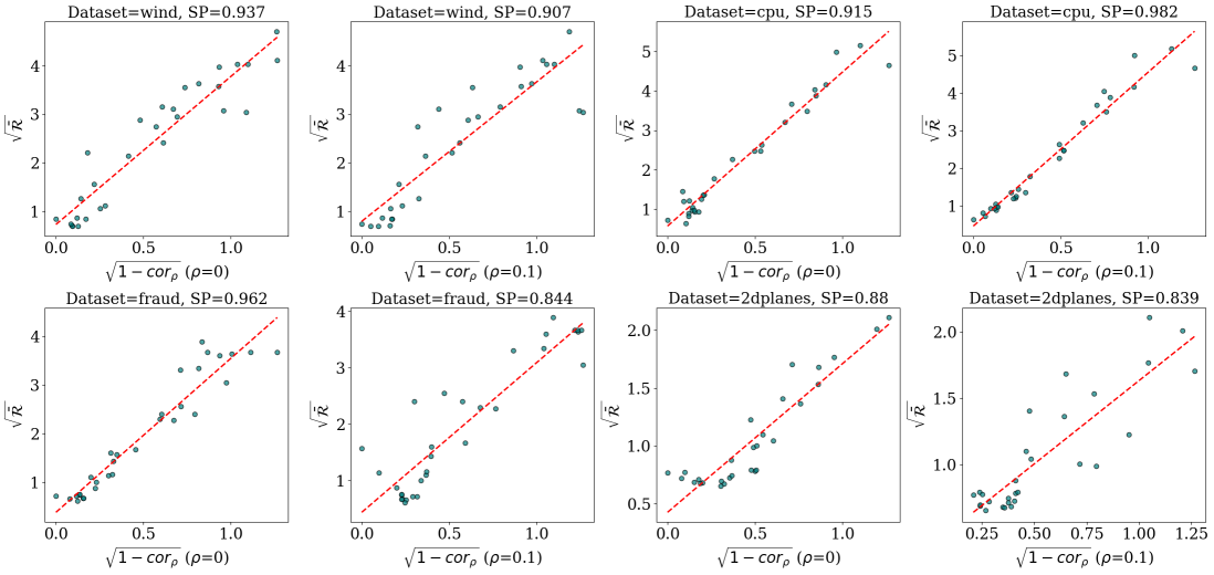
Figure 8: We investigate the correlation between the normalized fitting residual of MTM and the $\rho$-consistency index of the utility functions. The results for other values of $\rho$s are deferred to Appendix C. We vary different $\rho\in\{0,0.1\}$ and estimate the $\rho$-consistency index.

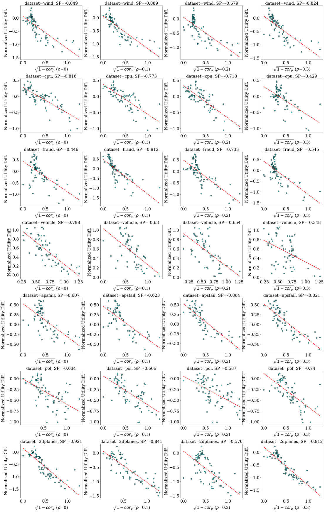
Figure 9: We investigate the correlation between the normalized fitting residual of MTM and the $\rho$-consistency index of the utility functions. The results for other values of $\rho$s are deferred to Appendix C. We vary different $\rho\in\{0,0.1,0.2,0.3\}$ and estimate the $\rho$-consistency index.

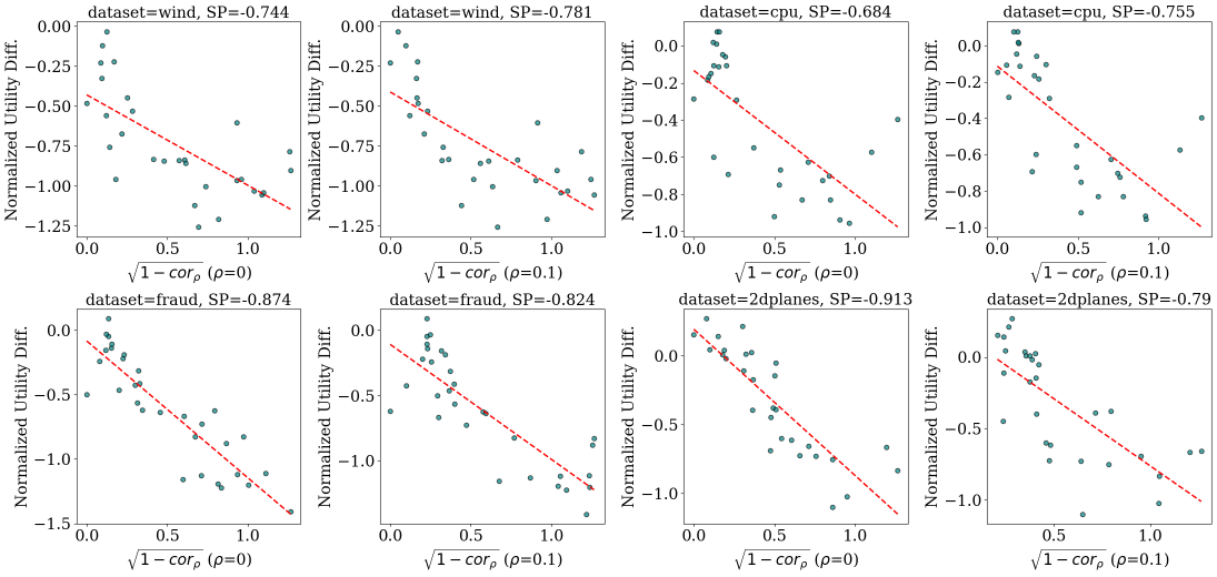
Figure 10: We investigate the correlation between the normalized fitting residual of MTM and the $\rho$-consistency index of the utility functions. The results for other values of $\rho$s are deferred to Appendix C. We vary different $\rho\in\{0,0.1\}$ and estimate the $\rho$-consistency index.

References

- Amiri et al. (2022) Amiri, M. M., Berdoz, F., and Raskar, R. Fundamentals of task-agnostic data valuation. arXiv preprint arXiv:2208.12354, 2022.
- Bilodeau et al. (2024) Bilodeau, B., Jaques, N., Koh, P. W., and Kim, B. Impossibility theorems for feature attribution. Proceedings of the National Academy of Sciences, 121(2):e2304406120, 2024.
- Bloch et al. (2021) Bloch, L., Friedrich, C. M., and Initiative, A. D. N. Data analysis with shapley values for automatic subject selection in alzheimer’s disease data sets using interpretable machine learning. Alzheimer’s Research & Therapy, 13:1–30, 2021.
- Castro et al. (2009) Castro, J., Gómez, D., and Tejada, J. Polynomial calculation of the shapley value based on sampling. Computers & Operations Research, 36(5):1726–1730, 2009.
- Dal Pozzolo et al. (2015) Dal Pozzolo, A., Caelen, O., Johnson, R. A., and Bontempi, G. Calibrating probability with undersampling for unbalanced classification. In 2015 IEEE Symposium Series on Computational Intelligence, pp. 159–166. IEEE, 2015.
- Das et al. (2022) Das, S., Sagarkar, M., Bhattacharya, S., and Bhattacharya, S. Checksel: Efficient and accurate data-valuation through online checkpoint selection. arXiv preprint arXiv:2203.06814, 2022.
- Dragan (2002) Dragan, I. C. On the inverse problem for semivalues of cooperative tu games. Technical report, University of Texas at Arlington, 2002.
- Duarte & Hu (2004) Duarte, M. F. and Hu, Y. H. Vehicle classification in distributed sensor networks. Journal of Parallel and Distributed Computing, 64(7):826–838, 2004.
- Dubey et al. (1981) Dubey, P., Neyman, A., and Weber, R. J. Value theory without efficiency. Mathematics of Operations Research, 6(1):122–128, 1981.
- Ghorbani & Zou (2019) Ghorbani, A. and Zou, J. Data shapley: Equitable valuation of data for machine learning. In International Conference on Machine Learning, pp. 2242–2251. PMLR, 2019.
- Ghorbani et al. (2020) Ghorbani, A., Kim, M., and Zou, J. A distributional framework for data valuation. In International Conference on Machine Learning, pp. 3535–3544. PMLR, 2020.
- Guu et al. (2023) Guu, K., Webson, A., Pavlick, E., Dixon, L., Tenney, I., and Bolukbasi, T. Simfluence: Modeling the influence of individual training examples by simulating training runs. arXiv preprint arXiv:2303.08114, 2023.
- Hammoudeh & Lowd (2021) Hammoudeh, Z. and Lowd, D. Simple, attack-agnostic defense against targeted training set attacks using cosine similarity. In ICML Workshop on Uncertainty and Robustness in Deep Learning, 2021.
- Ilyas et al. (2022) Ilyas, A., Park, S. M., Engstrom, L., Leclerc, G., and Madry, A. Datamodels: Predicting predictions from training data. arXiv preprint arXiv:2202.00622, 2022.
- Jia et al. (2019a) Jia, R., Dao, D., Wang, B., Hubis, F. A., Gurel, N. M., Li, B., Zhang, C., Spanos, C. J., and Song, D. Efficient task-specific data valuation for nearest neighbor algorithms. Proceedings of the VLDB Endowment, 2019a.
- Jia et al. (2019b) Jia, R., Dao, D., Wang, B., Hubis, F. A., Hynes, N., Gürel, N. M., Li, B., Zhang, C., Song, D., and Spanos, C. J. Towards efficient data valuation based on the shapley value. In The 22nd International Conference on Artificial Intelligence and Statistics, pp. 1167–1176. PMLR, 2019b.
- Jiang et al. (2023) Jiang, K. F., Liang, W., Zou, J., and Kwon, Y. Opendataval: a unified benchmark for data valuation. arXiv preprint arXiv:2306.10577, 2023.
- Just et al. (2022) Just, H. A., Kang, F., Wang, T., Zeng, Y., Ko, M., Jin, M., and Jia, R. Lava: Data valuation without pre-specified learning algorithms. In The Eleventh International Conference on Learning Representations, 2022.
- Koh & Liang (2017) Koh, P. W. and Liang, P. Understanding black-box predictions via influence functions. In International Conference on Machine Learning, pp. 1885–1894. PMLR, 2017.
- Kwon & Zou (2022) Kwon, Y. and Zou, J. Beta shapley: a unified and noise-reduced data valuation framework for machine learning. In International Conference on Artificial Intelligence and Statistics, pp. 8780–8802. PMLR, 2022.
- Kwon & Zou (2023) Kwon, Y. and Zou, J. Data-oob: Out-of-bag estimate as a simple and efficient data value. ICML, 2023.
- Kwon et al. (2021) Kwon, Y., Rivas, M. A., and Zou, J. Efficient computation and analysis of distributional shapley values. In International Conference on Artificial Intelligence and Statistics, pp. 793–801. PMLR, 2021.
- Lin et al. (2022) Lin, J., Zhang, A., Lécuyer, M., Li, J., Panda, A., and Sen, S. Measuring the effect of training data on deep learning predictions via randomized experiments. In International Conference on Machine Learning, pp. 13468–13504. PMLR, 2022.
- Mitchell et al. (2022) Mitchell, R., Cooper, J., Frank, E., and Holmes, G. Sampling permutations for shapley value estimation. 2022.
- Nohyun et al. (2022) Nohyun, K., Choi, H., and Chung, H. W. Data valuation without training of a model. In The Eleventh International Conference on Learning Representations, 2022.
- Northcutt et al. (2021) Northcutt, C. G., Athalye, A., and Mueller, J. Pervasive label errors in test sets destabilize machine learning benchmarks. In Thirty-fifth Conference on Neural Information Processing Systems Datasets and Benchmarks Track (Round 1), 2021.
- O’Donnell (2014) O’Donnell, R. Analysis of boolean functions. Cambridge University Press, 2014.
- Pandl et al. (2021) Pandl, K. D., Feiland, F., Thiebes, S., and Sunyaev, A. Trustworthy machine learning for health care: scalable data valuation with the shapley value. In Proceedings of the Conference on Health, Inference, and Learning, pp. 47–57, 2021.
- Paul et al. (2021) Paul, M., Ganguli, S., and Dziugaite, G. K. Deep learning on a data diet: Finding important examples early in training. Advances in Neural Information Processing Systems, 34:20596–20607, 2021.
- Pruthi et al. (2020) Pruthi, G., Liu, F., Kale, S., and Sundararajan, M. Estimating training data influence by tracing gradient descent. Advances in Neural Information Processing Systems, 33:19920–19930, 2020.
- Saunshi et al. (2022) Saunshi, N., Gupta, A., Braverman, M., and Arora, S. Understanding influence functions and datamodels via harmonic analysis. In The Eleventh International Conference on Learning Representations, 2022.
- Shapley (1953) Shapley, L. S. A value for n-person games. Contributions to the Theory of Games, 2(28):307–317, 1953.
- Sim et al. (2020) Sim, R. H. L., Zhang, Y., Chan, M. C., and Low, B. K. H. Collaborative machine learning with incentive-aware model rewards. In International Conference on Machine Learning, pp. 8927–8936. PMLR, 2020.
- Sim et al. (2022) Sim, R. H. L., Xu, X., and Low, B. K. H. Data valuation in machine learning:“ingredients”, strategies, and open challenges. In Proc. IJCAI, 2022.
- Søgaard et al. (2021) Søgaard, A. et al. Revisiting methods for finding influential examples. arXiv preprint arXiv:2111.04683, 2021.
- Sui et al. (2021) Sui, Y., Wu, G., and Sanner, S. Representer point selection via local jacobian expansion for post-hoc classifier explanation of deep neural networks and ensemble models. Advances in neural information processing systems, 34:23347–23358, 2021.
- Tang et al. (2021) Tang, S., Ghorbani, A., Yamashita, R., Rehman, S., Dunnmon, J. A., Zou, J., and Rubin, D. L. Data valuation for medical imaging using shapley value and application to a large-scale chest x-ray dataset. Scientific reports, 11(1):1–9, 2021.
- Tay et al. (2022) Tay, S. S., Xu, X., Foo, C. S., and Low, B. K. H. Incentivizing collaboration in machine learning via synthetic data rewards. In Proceedings of the AAAI Conference on Artificial Intelligence, volume 36, pp. 9448–9456, 2022.
- Wang & Jia (2023a) Wang, J. T. and Jia, R. Data banzhaf: A robust data valuation framework for machine learning. In International Conference on Artificial Intelligence and Statistics, pp. 6388–6421. PMLR, 2023a.
- Wang & Jia (2023b) Wang, J. T. and Jia, R. A note on” efficient task-specific data valuation for nearest neighbor algorithms”. arXiv preprint arXiv:2304.04258, 2023b.
- Wang et al. (2023) Wang, J. T., Zhu, Y., Wang, Y.-X., Jia, R., and Mittal, P. Threshold knn-shapley: A linear-time and privacy-friendly approach to data valuation. arXiv preprint arXiv:2308.15709, 2023.
- Wang et al. (2024) Wang, J. T., Mittal, P., and Jia, R. Efficient data shapley for weighted nearest neighbor algorithms. arXiv preprint arXiv:2401.11103, 2024.
- Wu et al. (2022) Wu, Z., Shu, Y., and Low, B. K. H. Davinz: Data valuation using deep neural networks at initialization. In International Conference on Machine Learning, pp. 24150–24176. PMLR, 2022.
- Xu et al. (2021) Xu, X., Wu, Z., Foo, C. S., and Low, B. K. H. Validation free and replication robust volume-based data valuation. Advances in Neural Information Processing Systems, 34:10837–10848, 2021.
- Yeh et al. (2018) Yeh, C.-K., Kim, J., Yen, I. E.-H., and Ravikumar, P. K. Representer point selection for explaining deep neural networks. Advances in neural information processing systems, 31, 2018.
- Yeh et al. (2022) Yeh, C.-K., Taly, A., Sundararajan, M., Liu, F., and Ravikumar, P. First is better than last for training data influence. arXiv preprint arXiv:2202.11844, 2022.
- Yeh & Lien (2009) Yeh, I.-C. and Lien, C.-h. The comparisons of data mining techniques for the predictive accuracy of probability of default of credit card clients. Expert systems with applications, 36(2):2473–2480, 2009.
- Yerushalmy (1947) Yerushalmy, J. Statistical problems in assessing methods of medical diagnosis, with special reference to x-ray techniques. Public Health Reports (1896-1970), pp. 1432–1449, 1947.
- Yokote et al. (2016) Yokote, K., Funaki, Y., and Kamijo, Y. A new basis and the shapley value. Mathematical social sciences, 80:21–24, 2016.
- Zheng et al. (2023) Zheng, K., Chua, H.-R., Herschel, M., Jagadish, H., Ooi, B. C., and Yip, J. W. L. Exploiting negative samples: A catalyst for cohort discovery in healthcare analytics. 2023.