Outlier Gradient Analysis:
Efficiently Improving Deep Learning Model Performance via Hessian-Free Influence Functions

Abstract

Influence functions offer a robust framework for assessing the impact of each training data sample on model predictions, serving as a prominent tool in data-centric learning. Despite their widespread use in various tasks, the strong convexity assumption on the model and the computational cost associated with calculating the inverse of the Hessian matrix pose constraints, particularly when analyzing large deep models. This paper focuses on a classical data-centric scenario—trimming detrimental samples—and addresses both challenges within a unified framework. Specifically, we establish an equivalence transformation between identifying detrimental training samples via influence functions and outlier gradient detection. This transformation not only presents a straightforward and Hessian-free formulation but also provides profound insights into the role of the gradient in sample impact. Moreover, it relaxes the convexity assumption of influence functions, extending their applicability to non-convex deep models. Through systematic empirical evaluations, we first validate the correctness of our proposed outlier gradient analysis on synthetic datasets and then demonstrate its effectiveness in detecting mislabeled samples in vision models, selecting data samples for improving performance of transformer models for natural language processing, and identifying influential samples for fine-tuned Large Language Models.

1 Introduction

Data-centric learning focuses on enhancing algorithmic performance from the perspective of the training data (Oala et al., 2023). In contrast to model-centric learning, which designs novel algorithms or optimization techniques for performance improvement with fixed training data, data-centric learning operates with a fixed learning algorithm while modifying the training data through trimming, augmenting, or other methods aligned with improving utility (Zha et al., 2023). Data-centric learning holds significant potential in many areas such as model interpretation, subset training set selection, data generation, noisy label detection, active learning, and others (Chhabra et al., 2024; Kwon et al., 2024).

The essence of data-centric learning lies in estimating data influence, also known as data valuation (Hammoudeh and Lowd, 2022), in the context of a learning task. Intuitively, the impact of an individual data sample can be measured by assessing the change in learning utility when training with and without that specific sample. This leave-one-out influence (Cook and Weisberg, 1982) provides a rough gauge of the relative data influence of the specific sample on the otherwise full fixed training set. On the other hand, Shapley value (Ghorbani and Zou, 2019; Jia et al., 2019), originating from cooperative game theory, quantifies the increase in value when a group of samples collaborates to achieve the learning goal. Unlike leave-one-out influence, Shapley value represents the weighted average utility change resulting from adding the point to different training subsets. Despite the absence of assumptions on the learning model, the aforementioned retraining-based methods incur significant computational costs, especially for large-scale data analysis and deep models (Hammoudeh and Lowd, 2022).

Diverging from the retraining-based category of approaches, influence functions assess data influence without requiring model retraining (Koh and Liang, 2017). They measure the effect of changing an infinitesimal weight of training samples based on a utility-evaluating function. While influence functions can be accurate or acceptable proxies for convex and certain shallow models (Koh and Liang, 2017), their applicability to deep models is constrained by the strong convexity assumption and the computational cost linked to calculating the inverse of the Hessian matrix (Basu et al., 2020a).

Our Contributions. In this paper, we delve into a classical data-centric scenario: trimming detrimental samples, also known as best subset selection (Bertsimas et al., 2016). We strive to tackle two significant challenges associated with influence functions within a unified framework. Our contributions are as follows:

• We build an equivalence transformation between identifying detrimental training samples via influence functions and outlier detection on the gradient space of samples, and propose our outlier gradient analysis approach. The theoretical transformation features a straightforward and Hessian-free formulation, and reduces the computational cost associated with the Hessian matrix and its inverse.

• Furthermore, our transformation relaxes the convex assumption of influence functions and extends their applicability from simple convex learning models to non-convex deep models via the Taylor expansion to high-order gradients. We utilize the first-order gradient for outlier analysis. Notably, it can be obtained during model training, and no additional high-order gradients are necessary for our outlier gradient analysis approach.

• Empirically we demonstrate that outlier gradient analysis can lead to performance improvements compared to existing influence-based approaches in deep learning while being computationally more efficient. We first demonstrate the efficacy of our framework compared to baselines on synthetic datasets. Subsequently, we showcase the usefulness of outlier gradient analysis on trimming mislabeled samples in vision datasets across a variety of noisy regimes. We also consider Natural Language Processing (NLP) applications by conducting experiments on data selection for fine-tuning deep transformer models such as RoBERTa Liu et al. (2019) and influential data identification for text generation tasks on fine-tuned Large Language Models (LLMs). As our results show, outlier gradient analysis obtains performance gains in a computationally efficient manner across diverse tasks, models, and application paradigms.

2 Related Work

Retraining-Based Influence Estimation. Influence estimation and data valuation approaches can be generally categorized as either retraining-based or gradient-based (Hammoudeh and Lowd, 2022). Retraining-based methods consist of the classical leave-one-out influence approach (Cook and Weisberg, 1982) which consists of removing one (or a group of) training sample(s) at a time, and retraining the model to measure sample influence via performance change. While useful as an ideal baseline, on deep models this is clearly an untenable influence approach as it necessitates computationally expensive model retrainings every time a sample is removed. Other representative methods include Shapley value approaches (Ghorbani and Zou, 2019; Jia et al., 2019; Kwon and Zou, 2022), which are model agnostic, but also computationally untenable for large datasets and deep models due to exponential time complexity. Computationally efficient approaches such as KNN-Shap (Jia et al., 2018) tend to make assumptions about the learning model and hence are not directly applicable to the (deep) models being considered. It is evident that for deep learning influence estimation, retraining-based approaches are not ideal, and hence, gradient-based methods are more suitable.

Gradient-Based Influence Estimation. For models trained using gradient descent, gradient-based influence approaches can be used to approximately estimate influence without requiring retraining. The seminal work in this category is that of Koh and Liang (2017), which utilizes a Taylor-series approximation and LiSSA optimization (Agarwal et al., 2017) to compute sample influences. However, the limiting assumption is that the model and loss function are convex, which is not true for deep models. Follow-up works such as representer point (Yeh et al., 2018) and Hydra (Chen et al., 2021) inherit these convexity assumptions and suffer from similar issues of applicability. Moreover, most modern influence function approaches (Schioppa et al., 2022; Feldman and Zhang, 2020) tend to be too computationally expensive for large models, and cannot run in reasonable time. More recently, Kwon et al. (2024) proposed DataInf, which efficiently computes influence even for large models simply be replacing the inverse Hessian computation with an easily computable closed-form expression, but their framework implicitly assumes convexity as well. Some approaches simply consider the gradients directly as a measure of influence (Pruthi et al., 2020; Charpiat et al., 2019). Other work in this domain has investigated traditional Hessian-based influence functions for relabeling samples (Kong et al., 2021), and how they can be scaled to use with LLMs (Grosse et al., 2023). Recent work has also investigated the role of the Hessian and convexity in influence estimation (Schioppa et al., 2024). In contrast, our work aims to circumvent these issues by operating on the gradient space in a skillful manner, and obviates the need for assuming model convexity. Hence, our work paves the way for an efficient and accurate influence estimation framework and adds to the “influence function toolset” for deep models and large datasets. Finally, recent work has also found that self-influence (influence computed on training samples) can be beneficial in detecting detrimental samples (Bejan et al., 2023; Thakkar et al., 2023) so we compare our proposed method with these approaches as well.

Miscellaneous Data-Centric Learning. Many works in the data-centric learning domain study other relevant research questions. For instance, datamodels (Ilyas et al., 2022) also estimate training sample contributions, but only for one test sample at a time. Data efficiency approaches (Jain et al., 2023; Paul et al., 2021; Killamsetty et al., 2021) aim to accelerate deep learning training time via subset selection. Data pruning approaches based on novel approximations for leave-one-out influence estimation (Tan et al., 2024) and the model’s generalization gap (Yang et al., 2022) have also been proposed. Model pruning via generalized influence functions has also been studied in (Lyu et al., 2023). Antidote data augmentation (Chhabra et al., 2022; Li et al., 2023) methods aim to generate synthetic data samples to improve model performance, whereas feature selection approaches (Hall, 1999; Cai et al., 2018) seek to optimize the feature space to only those important for model performance. Active learning (Cohn et al., 1996) methods aim to iteratively identify optimal samples to annotate given a large unlabeled training data pool (Liu et al., 2021; Nguyen et al., 2022; Wei et al., 2015). Finally, works on poisoning attacks seek to analyze model robustness by perturbing training set samples (Solans et al., 2021; Mehrabi et al., 2021; Chhabra et al., 2023) under natural input constraints. The study of training sample influence has also been extended to recent generative models, such as diffusion models (Dai and Gifford, 2023), through the use of ensembles.

3 Proposed Approach

We first introduce influence functions conceptually and outline their classical application in identifying detrimental samples. We then detail our equivalence transformation by converting the research question into a gradient space outlier analysis problem. Subsequently, we provide insights for extending influence functions to non-convex learning models and propose our outlier gradient analysis approach.

3.1 Preliminaries on Influence Functions

Let $T$$=$$\{z_{i}\}_{i=1}^{n}$ be a training set, where $z_{i}$ $=$$(x_{i},y_{i})$ includes the input space feature $x_{i}$ and output space label $y_{i}$. A classifier trained using empirical risk minimization on the empirical loss $\ell$ can be written as: $\hat{\theta}$$=$$\operatorname*{arg\,min}_{\theta\in\Theta}\frac{1}{n}\sum_{i=1}^{n}\ell(z_{i};\theta)$. Influence functions (Cook and Weisberg, 1982; Hampel, 1974; Martin and Yohai, 1986) measure the effect of changing an infinitesimal weight of training samples, based on a function that evaluates model utility. Downweighting a training sample $z_{j}$ by a very small fraction $\epsilon$ leads to a model parameter: $\hat{\theta}(z_{j};-\epsilon)=\operatorname*{arg\,min}_{\theta\in\Theta}\frac{1}{n}(\sum_{i=1}^{n}\ell(z_{i};\theta)$$-$$\epsilon\ell(z_{j};\theta))$. By evaluating the limit as $\epsilon$ approaches 1, the seminal work of Koh and Liang (2017) provides an estimation for the influence score associated with the removal of $z_{j}$ from the training set in terms of training/validation loss as follows:

$$\mathcal{I}(z_{j})=-\sum_{z\in T/V}\nabla_{\hat{\theta}}\ell(z;\hat{\theta})^{\top}\mathbf{H}^{-1}_{\hat{\theta}}\nabla_{\hat{\theta}}\ell(z_{j};\hat{\theta}),$$ (1)

where $T/V$ denotes the training/validation set, $\nabla_{\hat{\theta}}\ell(z_{j};\hat{\theta})$ is the gradient of the loss with respect to network parameters, and $\mathbf{H}_{\hat{\theta}}$$=$$\sum_{i=1}^{n}\nabla_{\hat{\theta}}^{2}\ell(z_{i};\hat{\theta})$ denotes the Hessian matrix.

One key application of influence functions lies in identifying detrimental samples. An intuitive approach involves training the model both with and without the specific training sample and assessing the resulting changes using metrics like training/validation loss. In other words, if the performance improves when excluding a particular sample, it is deemed detrimental to the learning task. By computing the influence score without needing to retrain the model, one can estimate the impact of a sample to assess if it is beneficial or detrimental, as follows:

$$\tilde{\mathcal{I}}(z_{j})=\begin{cases}0\ \textup{(Detrimental Sample)}&\mathcal{I}(z_{j})<0.\\ 1\ \textup{(Beneficial Sample)}&\mathcal{I}(z_{j})\geq 0.\end{cases}$$ (2)

$\tilde{\mathcal{I}}(z_{j})$ can be regarded as a the discrete version of $\mathcal{I}(z_{j})$. Specifically, a positive value for $\mathcal{I}(z_{j})$ means that removing the sample $z_{j}$ enhances the model’s utility, and that $z_{j}$ is a detrimental sample.

While influence functions offer a swift estimation of the training sample effect without the need for costly model retraining, their practical applications are constrained by two prominent drawbacks. The initial limitation lies in the necessity of a strictly convex loss function to guarantee the existence of the inverse of the Hessian matrix. The second challenge pertains to the considerable computational expense associated with calculating the inverse of the Hessian matrix. For the first challenge, several possible solutions exist: (1) a linear model can be used as a surrogate on the embeddings obtained via the non-convex model (Chhabra et al., 2024); (2) a damping term can be added to the non-convex model such that its Hessian becomes positive definite and invertible (Han et al., 2020); and (3) for certain tasks specific or second-order influence functions can be derived (Basu et al., 2020b; Alaa and Van Der Schaar, 2020). For the second challenge, various matrix inverse techniques are employed to expedite the computation process, including LiSSA optimization (Koh and Liang, 2017) and swapping the order of the matrix inversion (Kwon et al., 2024). Considerable efforts have been dedicated to addressing the aforementioned challenges with promising results; this paper aims to unify and confront both challenges under a single framework. We endeavor to present a straightforward and elegant solution for extending influence functions to non-convex loss functions.

3.2 Bridging Influence Estimation and Outlier Analysis

Now we transform the problem of identifying detrimental samples via influence estimation to an outlier analysis problem in the gradient space. Upon scrutinizing the influence estimation of $z_{j}$ in Eq. (1), it becomes evident that the influence score is the result of three terms, with the first two being constant across all training samples and independent of $z_{j}$. While all three terms contribute to the concrete value of the influence score, it is the final term $\nabla_{\hat{\theta}}\ell(z_{j};\hat{\theta})$ that assumes a decisive role in determining whether $z_{j}$ is a beneficial or detrimental sample. This is because only the third term has $z_{j}$ as input. With the following observation, we can build the connection between identifying detrimental samples via influence estimation and outlier analysis.

Observation 3.1.

The majority of training samples positively contribute to the model’s utility, with only a small subset (with respect to the overall size of the training set) exhibiting detrimental effects.

Clearly, Observation 3.1 holds true as the empirical loss is an average of error between predictive and true values over all training samples. Hence, detrimental samples can be regarded as outliers compared to the beneficial sample majority. Based on Observation 3.1 and the decisive role of $\nabla_{\hat{\theta}}\ell(z_{j};\hat{\theta})$ in influence estimation, we have the following proposition:

Proposition 3.2.

There exists an outlier analysis algorithm for detecting outliers in the gradient space of samples, such that determining whether a training sample beneficially or detrimentally impacts model utility through influence estimation is equivalent to applying this outlier analysis algorithm on the gradient space.

Proposition 3.2 establishes a conceptual equivalence transformation between the identification of detrimental training samples via influence estimation and the detection of outliers in the gradient space. This theoretical transformation not only features a straightforward and Hessian-free formulation, reducing the computational cost associated with the Hessian matrix and its inverse, but also yields profound insights into the role of the gradient in sample impact beyond model optimization. Furthermore, this transformation relaxes the convexity assumption of influence functions. While the influence estimation in Eq. (1) is a first-order Taylor expansion, sufficient for convex loss functions, non-convex loss functions demand higher-order Taylor expansions for accurate estimation (Basu et al., 2020b; Alaa and Van Der Schaar, 2020). The higher-order Taylor expansion of influence estimation is the summation of the product of three terms with different orders, where the first term $\sum_{z\in T/V}\nabla_{\hat{\theta}}\ell(z;\hat{\theta})^{\top}$ is a constant. In a similar vein, our transformation for high-order Taylor extensions renders all Hessian-related terms, including their high-order formulations and inverses, constants as well. This characteristic alleviates the need for gradients with different orders in determining whether a sample is beneficial or detrimental, even for non-convex models.

3.3 Our Approach: Outlier Gradient Analysis

Algorithm 1 : Outlier Gradient Analysis and Trimming

1:Input: Training set $T$, loss $\ell$, trained model param $\hat{\theta}$, outlier analysis algorithm $\mathcal{A}$, trimming budget $k$

2:Output: Set $L$ containing beneficial/detrimental sample labels, Trimmed training set $T^{*}$

3:initialize $\mathcal{G}\leftarrow\emptyset,T^{*}\leftarrow\emptyset$.

4:$\mathcal{G}\leftarrow\mathcal{G}\cup\{\nabla_{\hat{\theta}}\ell(x_{i},y_{i};\hat{\theta})\};\forall(x_{i},y_{i})\in T$.

5:$L\leftarrow\mathcal{A}(\mathcal{G},k)$.

6:$T^{*}\leftarrow T^{*}\cup\{x_{i}\};\forall\,L_{i}\textit{ is not an outlier}$.

7:return $L,T^{*}$.

As demonstrated in Proposition 3.2, outlier analysis can effectively evaluate the discrete influence of training samples. Notably, we can circumvent the need for computing and inverting the Hessian and adapt influence function to non-convex deep models while still measuring discrete influence via Eq. (2). The primary contribution and discovery of our work lies in the realization that simple and efficient outlier analysis techniques can be applied to the gradient space for a discrete estimation of which samples are beneficial or detrimental to the model’s utility.

As Proposition 3.2 does not prescribe a specific outlier detection algorithm, one of our choices for outlier analysis is the Isolation Forest (iForest) (Liu et al., 2008) algorithm due to several factors. Firstly, iForest boasts a linear time complexity with a low constant, requiring minimal memory, rendering it well-suited for handling the high-dimensional gradient space inherent in deep models. Secondly, iForest constructs an ensemble of iTrees, where each iTree builds partial models and employs sub-sampling, demonstrating the ability to identify a suitable subspace for the detection of detrimental samples. Thirdly, iForest is known for its simplicity and effectiveness in identifying outliers that are non-linearly separated from inliers. Along with iForest, we also consider two simple outlier analysis approaches based on L1-norm and L2-norm thresholding, that work well in practice (Knorr et al., 2000).

Upon obtaining outlyingness labels through the application of an outlier detection algorithm to the gradient space, denoted as the set $L$, we can assess the influence of training samples on model performance. Subsequently, we then trim $k$ (the designated deletion budget) detrimental training samples. Retraining the model on this pruned sample set leads to potential performance improvements. The approach is outlined in Algorithm 1.

4 Correctness Verification on Synthetic Data

We seek to validate the correctness of our proposed idea and showcase the effectiveness of our outlier gradient analysis method on two synthetic 2D toy datasets and two models for binary classification in Figure 1. In this figure, subfigures A-D present a linear dataset employing a Logistic Regression model, while subfigures E-H exhibit a non-linear dataset utilizing a non-convex Multilayer Perceptron (MLP) model as the base model. Specifically, subfigures A and B depict the training and test sets of a linearly separable dataset comprising 150 and 100 samples, respectively. Notably, the training set includes 10 manually generated noisy samples with misspecified labels. Subfigure C displays the influence score of each training sample, computed using Eq. (1), and subfigure D provides a visualization of the gradient space. Similarly, subfigures E and F represent the training and test sets of the two half moons dataset, with the training set consisting of 250 samples and the test set of 100 samples, equally distributed between two classes. The training set in this case also contains 20 noisy samples. Subfigures G and H showcase the influence score and gradient space of the non-convex case.

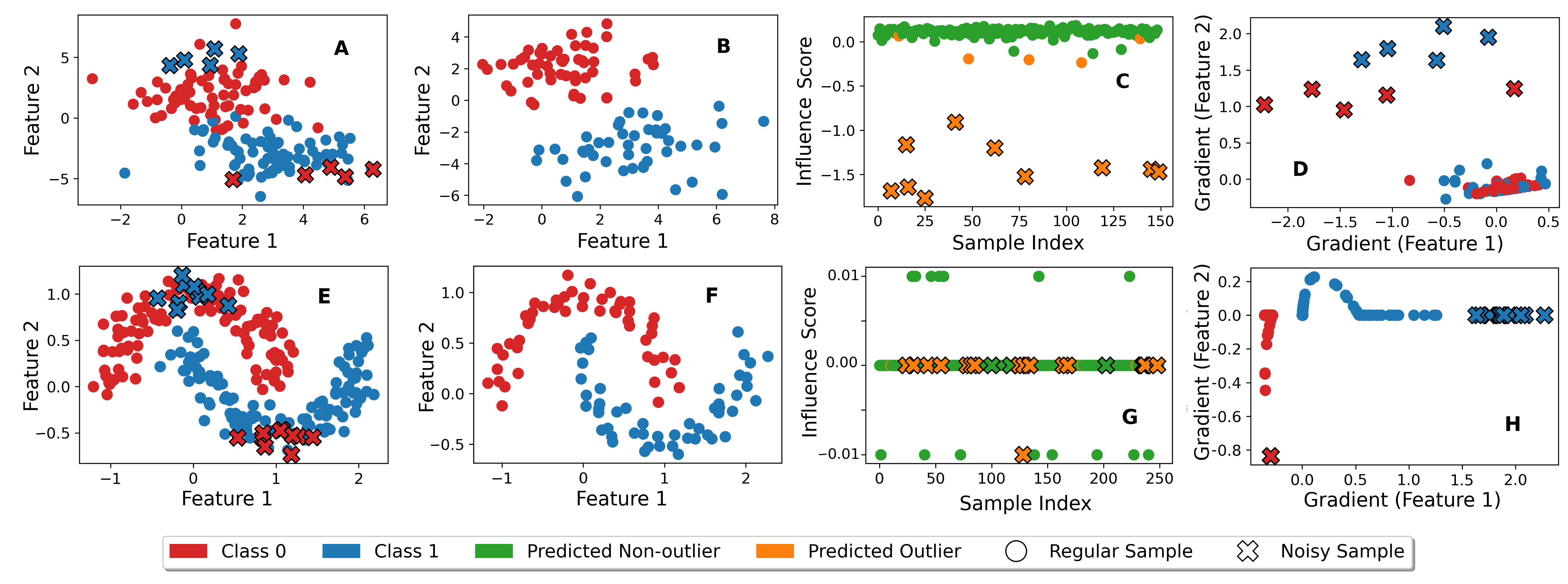
Figure 1: Illustrating our outlier gradient analysis approach on two synthetic datasets and convex/non-convex models. Subfigures A-D showcase our outlier gradient analysis approach on a 2D linearly separable synthetic dataset. This dataset includes a small subset of detrimental samples with incorrect labels used to train a Logistic Regression binary classification model. Meanwhile, subfigures E-H depict our outlier gradient analysis on a non-linear synthetic dataset with mislabeled samples employed in training a Multilayer Perceptron (MLP) neural network. In subfigures A and E, the training sets are represented with class labels 0 (red) and 1 (blue) in the convex and non-convex cases, respectively. Detrimental samples with incorrect class labels are marked with $\times$, while regular samples are marked with $\circ$. Subfigures B and F denote the test sets used to evaluate model performance in the convex and non-convex scenarios. Subfigures C and G display the influence scores calculated by Eq. (1). Upon running our outlier analysis algorithm on the gradient space of the linear convex model (subfigure C), most detrimental samples are identified (depicted in orange), while regular points are considered inliers. Notably, these outliers exhibit lower influence scores, as influence functions prove accurate for convex models. In contrast, subfigure G demonstrates that influence scores are not reliable indicators for detecting detrimental samples in the non-convex case. However, after applying outlier analysis on the gradient space of the non-convex MLP model, most detrimental samples are detected (depicted in orange). Subfigures D and H showcase the gradient space obtained for each sample from the Logistic Regression and MLP models, respectively. It is evident that the outlier samples correspond to detrimental samples with mislabeled classes, which is linearly or non-linearly separated from inliers. Note that the benefits of outlier gradient trimming can be clearly observed—removing predicted outlier samples via iForest and retraining the MLP enhances classification performance from $90\%\rightarrow 96\%$ on the test set (refer to Table 1).

In the linear case, as illustrated in subfigure C, the influence score proves to be a reliable indicator for distinguishing detrimental samples from beneficial ones. Notably, detrimental samples exhibit large negative scores, while other samples display positive or nearly zero values. Additionally, subfigure D affirms that these detrimental samples are distinctly separated in the gradient space, confirming the validity of the equivalent transformation outlined in Proposition 3.2. However, the limitations of influence scores become evident in the context of non-convex models, as observed in subfigure G, where the influence scores of detrimental samples are mixed with those of normal ones. Nevertheless, in the gradient space illustrated in subfigure H, the detrimental samples are effectively isolated from inliers. Notably, our method does not rely on the Hessian for computing influence; instead, it operates directly on the gradient space using outlier analysis techniques. This highlights that our gradient outlier analysis approach effectively relaxes the convexity assumption associated with influence functions.

Table 1: Outlier detection and classification performance of noisy label correction and influence-based approaches including our proposed outlier gradient trimming on the two half moons dataset (top-2 performers in bold).

Method	Outlier Detection Accuracy (%)	Classification Post-Trimming (%)
Multilayer Perceptron	-	90.0
Normalized Margin Northcutt et al. (2021)	82.0	89.0
Self-Confidence Müller and Markert (2019)	82.0	89.0
Confidence Entropy Kuan and Mueller (2022)	82.0	89.0
Exact Hessian Cook and Weisberg (1982)	90.0	90.0
Gradient Tracing Pruthi et al. (2020)	82.0	91.0
LiSSA Koh and Liang (2017)	82.0	91.0
DataInf Kwon et al. (2024)	82.0	91.0
Self-LiSSA Bejan et al. (2023)	82.0	90.0
Self-DataInf	90.0	87.0
Outlier Gradient (L1)	98.0	87.0
Outlier Gradient (L2)	98.0	87.0
Outlier Gradient (iForest)	96.0	96.0

We also conduct a quantitative evaluation to assess the advantages of our approach compared to three recently proposed noisy label correction methods and six influence function-based approaches, as detailed in Table 1. Specifically, we measure ground-truth outlier predictive accuracy and the performance gain achieved by removing detrimental samples. For noisy label correction approaches we consider: Normalized Margin (Northcutt et al., 2021), Self-Confidence (Müller and Markert, 2019), and Confidence-Weighted Entropy (Kuan and Mueller, 2022). The influence function approaches include computing the Hessian exactly (Cook and Weisberg, 1982), using the Hessian-free gradient tracing approach by (Pruthi et al., 2020), LiSSA-based optimization (Koh and Liang, 2017), the recently proposed influence estimation approach DataInf (Kwon et al., 2024), self-influence using LiSSA as in (Bejan et al., 2023), and self-influence using DataInf. We compute influences only using the training samples and performance is measured on the test set.

Our outlier gradient analysis approaches demonstrate high accuracy in identifying mislabeled outliers (96-98%), outperforming all three noisy label correction baselines (only 82% accuracy) and among influence baselines, all exhibit similar performance except for exact Hessian computation, which attains 90% accuracy. Next, we evaluate model performance gain by removing detected outlier samples and retraining the MLP on the trimmed dataset. Here the benefits of our iForest outlier gradient analysis can be observed, as it increases performance from 90% to 96% while the overtly simple L1/L2-norm outlier analysis approaches are not as effective. The other baselines exhibit performance variations between 89-91%. This emphasizes the effectiveness of our iForest approach, while exhibiting low time complexity (refer to Appendix B.3 for details on computational complexity).

5 Noisy Label Correction for Vision Datasets

Table 2: Accuracy (5 runs) on CIFAR-10N and CIFAR-100N for a ResNet-34 model trained via cross entropy and performance post trimming using noisy label correction approaches and influence-based methods, including our outlier gradient analysis (top-2 performers in bold).

Method	CIFAR-10N			CIFAR-100N
	Aggregate	Random	Worst	Noisy100
Cross Entropy	90.87	89.17	82.27	57.36
Normalized Margin Northcutt et al. (2021)	91.33	90.06	83.57	60.94
Self-Confidence Müller and Markert (2019)	91.38	90.09	83.65	60.51
Confidence Entropy Kuan and Mueller (2022)	91.11	90.05	83.63	60.62
Gradient Tracing Pruthi et al. (2020)	91.47	89.98	83.38	60.73
LiSSA Koh and Liang (2017)	91.49	90.05	83.38	60.48
DataInf Kwon et al. (2024)	91.46	90.05	83.40	60.70
Self-LiSSA Bejan et al. (2023)	92.07	89.58	83.01	59.48
Self-DataInf	91.41	89.81	83.15	60.56
Outlier Gradient (L1)	91.86	90.66	84.20	60.32
Outlier Gradient (L2)	92.21	90.25	82.99	61.40
Outlier Gradient (iForest)	91.36	90.20	83.72	60.99

Here we demonstrate the effectiveness of our approach in addressing noisy label correction using the CIFAR-10N and CIFAR-100N real-world noisy label datasets (Wei et al., 2022). These datasets stem from the original CIFAR-10 and CIFAR-100 datasets (Krizhevsky et al., 2009), but introduce label inaccuracies due to crowdsourced labeling. CIFAR-10N has 3 different noise settings: Aggregate, Random, and Worst– these correspond to obtaining the label using majority voting across 3 annotators, the first annotator label, and selecting the worst annotator label, respectively. CIFAR-100N only has a single noise setting.

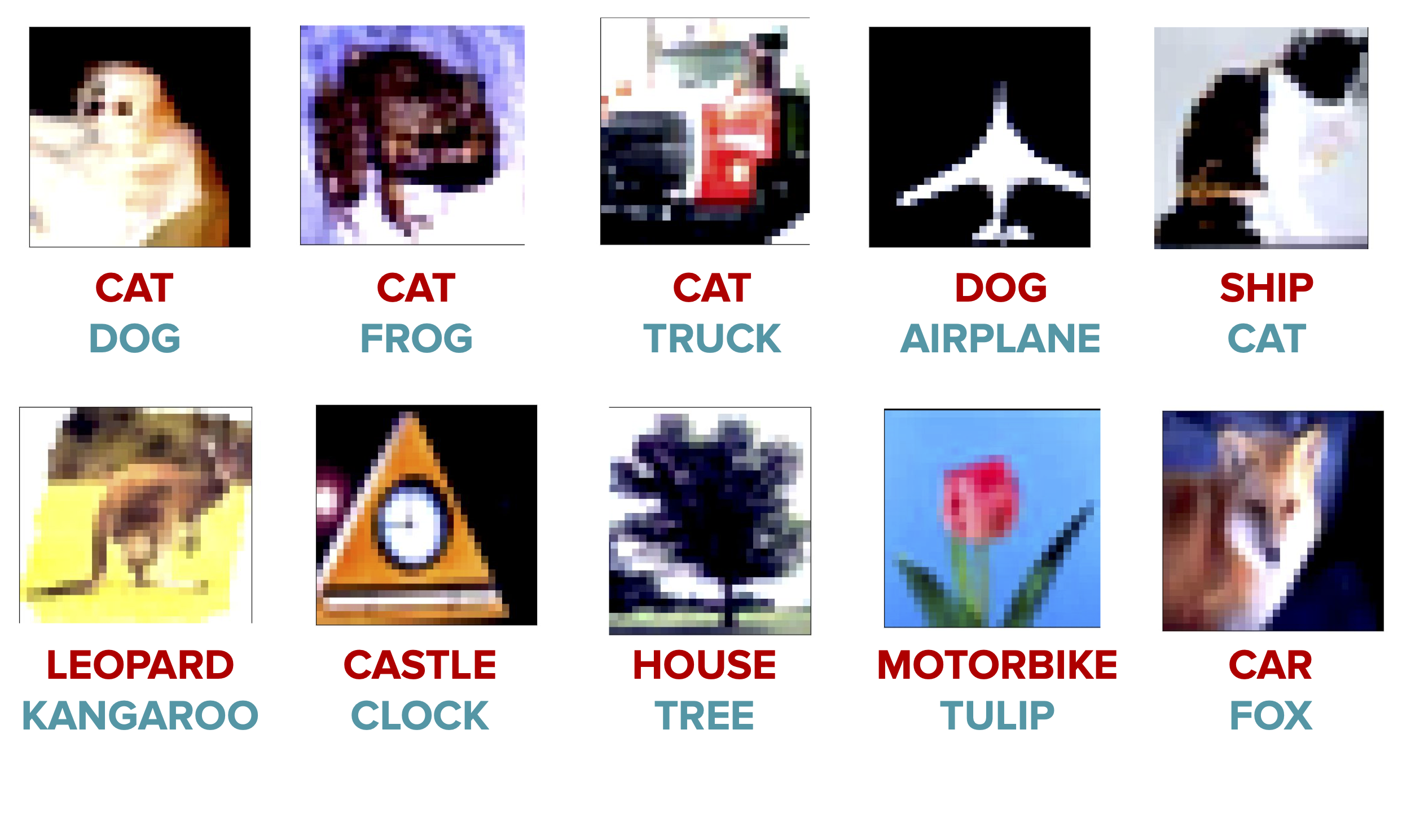
Figure 2: Examples of detrimental noisy samples detected using our proposed outlier gradient analysis. Top row: CIFAR-10N; bottom row: CIFAR-100N. Top label (red): noisy label; bottom label (green): correct class.

Table 2 shows the accuracy performance of our outlier gradient trimming approaches (iForest, L1/L2-norm) compared to label correction approaches and influence-based baselines covered in the previous section. Exact Hessian computation is excluded due to its computationally intractability for large datasets. Our outlier gradient analysis methods consistently outperform other baselines across diverse noise settings and datasets. Notably, even in challenging scenarios like the Worst noise setting in CIFAR-10N (40.21% noise rate), our approaches are the top performers– L1-norm based outlier analysis achieves highest accuracy gain, improving from 82.27% (vanilla ResNet-34) to 84.20%. Similar superior performance is observed in the Random noise setting (17.23% noise rate), where L2-norm outlier analysis achieves a final accuracy of 90.25% compared to original cross-entropy accuracy of 89.17% and in CIFAR-100N, where it attains the highest performance of 61.40%, surpassing the cross-entropy performance of 57.36%. In the CIFAR-10N Aggregate noise setting (noise rate 9.03%), outlier gradient analysis is again the top performer. Due to space constraints, we omit standard deviations from Table 2, but these are provided in Appendix B.1.

Additionally, visual examples of mislabeled samples detected by our outlier gradient analysis approach (iForest) are provided in Figure 2. All displayed images contain mislabeled samples, and their removal from the training set contributes to improved model performance on the test set. In Table 2, we set the trimming budget for outlier gradient analysis ($k$) at 5% of the training data size. An empirical justification for this choice is provided in Appendix B.2, where we vary the outlier budget and measure test set accuracy. We also conduct ablations on the iForest parameters in Appendix B.4 and provide running time experiments in Appendix B.3 to benchmark the computational efficiency of our approach. We provide experiments with ResNet-18 He et al. (2016) as the base model in Appendix B.6 and on ImageNet Deng et al. (2009) in Appendix B.5 showing similar trends.

6 Data Selection for Fine-tuning NLP Models

We conduct experiments on data selection for fine-tuning on NLP models, following the experiment setup by Kwon et al. (2024) for DataInf, where the RoBERTa transformer model (Liu et al., 2019) is fine-tuned on four binary GLUE datasets (Wang et al., 2018): QNLI, SST2, QQP, and MRPC. More details on these datasets and RoBERTa are provided in Appendix A. To assess if influence-based methods can enhance NLP model performance via Low Rank Adaptation (LoRA) (Hu et al., 2022) fine-tuning, Kwon et al. (2024) introduce noisy versions of all four datasets by flipping the binary label for 20% randomly chosen training data samples.

The goal of the data selection task is to select the best representative subset of the training data so that performance is maximized on an unseen test set. Specifically, 70% of the most beneficial samples are selected according to each influence computation approach, and the model is fine-tuned for 10 epochs and rank of LoRA matrix is set to 4. Then, as the model trains over each epoch, performance is measured on the unseen test set. Clearly, for fairness, the sample influence is computed only using the training set, and the test set remains unknown until inference.

The results over three runs are presented in Figure 3 for all four GLUE datasets. We only show trends for iForest based outlier gradient analysis to aid visualization since performance is similar for the L1/L2-norm methods. It can be seen that our outlier gradient trimming approach markedly outperforms all other baselines but the Self-LiSSA (Bejan et al., 2023) self-influence baseline is competitive with our approach. More specifically, outlier gradient analysis achieves slightly better test set results on QNLI, SST2, QQP, and on MRPC, Self-LiSSA and outlier gradient analysis are on par with each other. Here, we would like to emphasize that despite competitive performance, our outlier gradient analysis is orders of magnitude faster than Self-LiSSA, as shown in experiments of Appendix B.3. These results highlight the effectiveness of our proposed outlier gradient analysis/trimming approach in selecting relevant data for fine-tuning NLP models while being more computationally efficient.

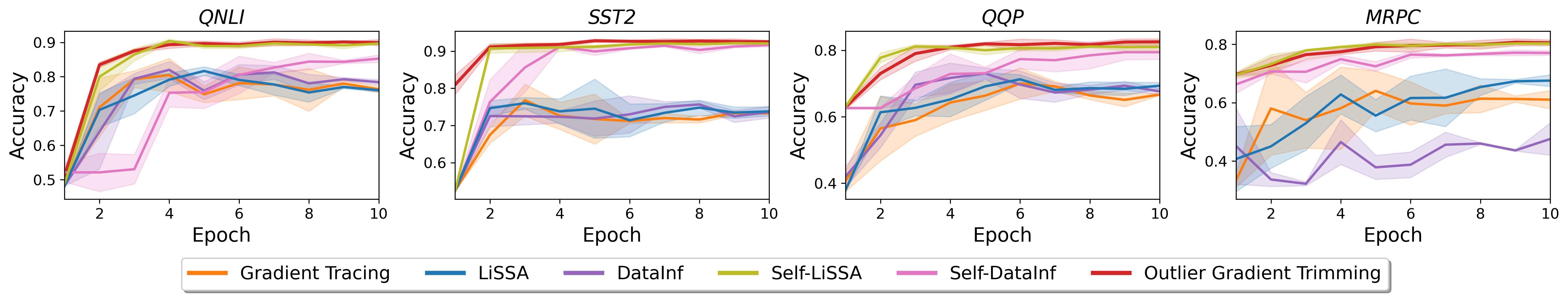
Figure 3: Performance of the data selection task utilizing outlier gradient trimming and other influence-based baselines for fine-tuning RoBERTa via LoRA over 3 runs.

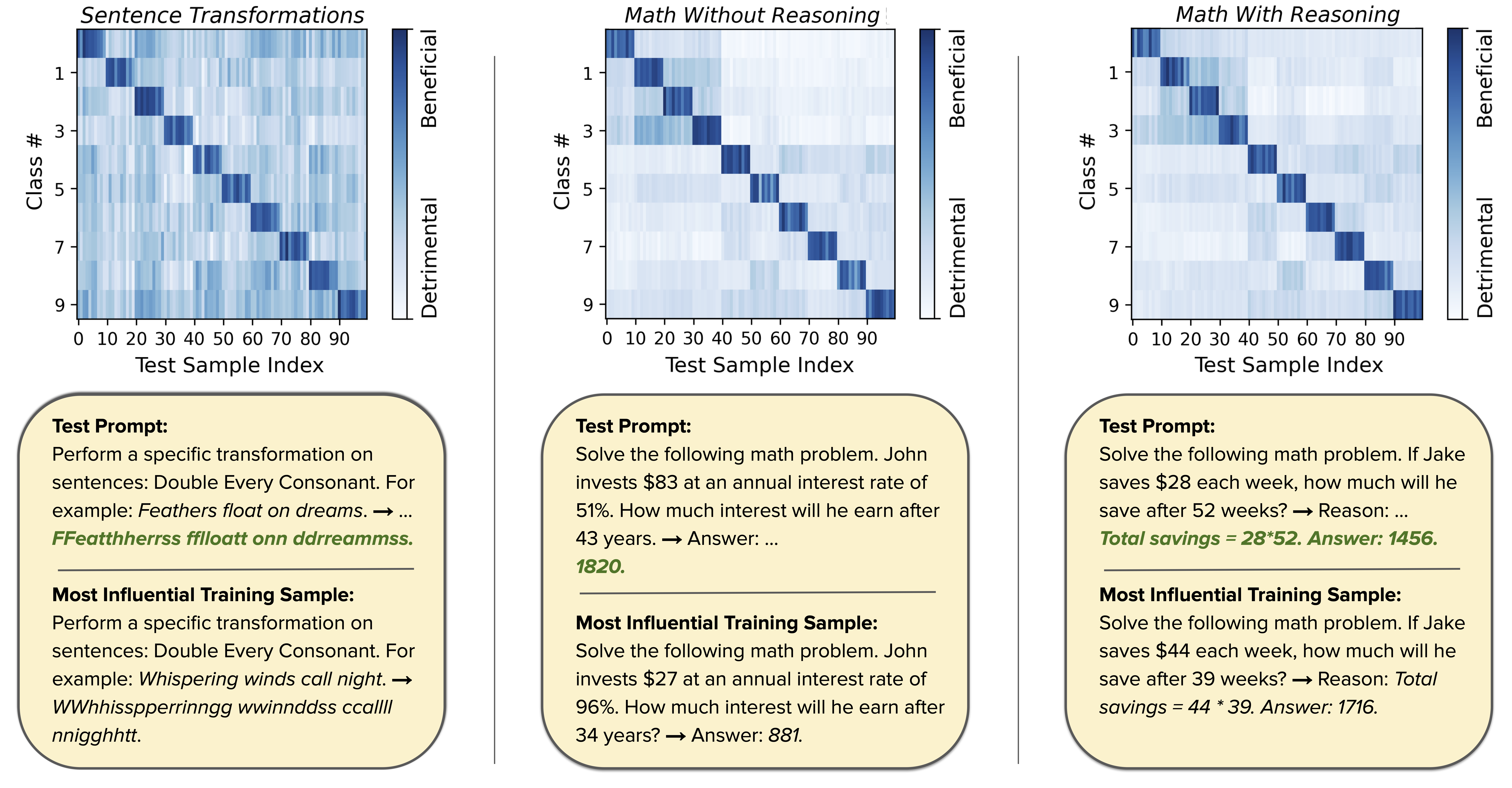
Figure 4: Quantitative and qualitative results for outlier gradient analysis on LLM influential data identification benchmarks.

7 Influential Data Identification for LLMs

We demonstrate the effectiveness of our proposed outlier gradient analysis in identifying beneficial/detrimental samples for Large Language Models (LLMs), using benchmarks from DataInf (Kwon et al., 2024). Since LLMs are primarily employed for text generation tasks, and not text classification, we cannot directly measure the benefits of influence estimation as we did previously for RoBERTa using the GLUE datasets. Instead, Kwon et al. (2024) resort to an indirect measurement of influence for LoRA fine-tuned LLMs. Specifically, they seek to assess what training set prompts (used for fine-tuning) are identified as most influential for a given unseen test prompt. The robustness and effectiveness of influence estimation are gauged based on whether the identified training set prompts belong to the same class category as the given test prompt. We utilize the three benchmark datasets introduced in DataInf (Kwon et al., 2024): Sentence Transformations, Math Without Reasoning, and Math With Reasoning, to conduct the influential data identification experiment on the Llama-2-13B-chat LLM. For each of the influence identification benchmark datasets, there are 900 training samples for LoRA fine-tuning, and 10 categories or classes of task types with 90 samples belonging to each class. For each dataset there are 100 test set prompts and with 10 test set prompts per class category.

Table 3: AUC/Recall for outlier gradient analysis and baselines for influential class detection on 3 text generation tasks on Llama2-13B-chat LLM.

Task	Method	Class Detection (AUC)	Class Detection (Recall)
Sentence Transformations	Gradient Tracing (Pruthi et al., 2020)	0.999 ± 0.001	0.982 ± 0.032
	DataInf (Kwon et al., 2024)	1.000 ± 0.000	0.996 ± 0.012
	Outlier Gradient Analysis	1.000 ± 0.000	1.000 ± 0.000
Math Problems Without Reasoning	Gradient Tracing (Pruthi et al., 2020)	0.724 ± 0.192	0.241 ± 0.385
	DataInf (Kwon et al., 2024)	0.999 ± 0.005	0.993 ± 0.046
	Outlier Gradient Analysis	1.000 ± 0.000	1.000 ± 0.000
Math Problems With Reasoning	Gradient Tracing (Pruthi et al., 2020)	0.722 ± 0.192	0.226 ± 0.376
	DataInf (Kwon et al., 2024)	0.999 ± 0.004	0.990 ± 0.049
	Outlier Gradient Analysis	1.000 ± 0.000	1.000 ± 0.000

In Kwon et al. (2024), to predict the most influential training samples given a test set prompt, the authors assign a pseudo label to every data point in the training set (1 if it is in the same class/task category as the test data prompt, or 0 otherwise). This set serves as a ground-truth for measuring performance of influence functions in identifying influential data samples. Next, they calculate the Area Under the Curve (AUC) by comparing the absolute values of the influence function (for each training set prompt corresponding to a given test prompt) with these pseudo labels. Clearly, a high AUC signifies that training data samples from the same category have a significant influence on the given test prompt. The average AUC across all test data points is then recorded, and is denoted as the Class Detection (AUC) metric. Additionally, another metric is used– for every test data prompt, the authors determine if the proportion of training data prompts belonging to the same class/category are within the top 90 (# of training prompts in each category) influential samples. The average % across all test data points is calculated and this metric is denoted as Class Detection (Recall). A higher recall indicates more effective influence estimation.

In our proposed outlier gradient analysis approach, we initially used outlyingness labels directly for identifying detrimental samples. However, for a more fine-grained analysis, we now require detailed outlyingness values. To achieve this, we require outlyingness scores and hence, train 10 individual iForest estimators for each class prompt category, as the ultimate objective is to use outlier gradient analysis for prompt class detection. Each class’s iForest estimator is trained solely on the gradient space of training prompts from that category. Subsequently, for each test set prompt, we utilize each iForest estimator to generate an outlier score based on the gradient space of that test sample. This enables us to conduct the influential data identification experiment for our proposed method.

The results of this experiment are presented in Table 3. Our outlier gradient analysis performs exceptionally well on this task, achieving perfect scores for both AUC and Recall. It outperforms DataInf and Gradient Tracing, with LiSSA omitted as it fails to converge due to instability on LLMs (Kwon et al., 2024). Self-influence baselines also cannot be used since a similarity matrix with test prompts needs to be constructed. Figure 4 further illustrates the individual influence predictions, with darker colors indicating lower outlier score magnitudes. The heatmaps correspond to each of the three benchmark datasets, with test samples ordered sequentially based on their class category. The accurate influence estimation is evident from the highest influence values along the diagonal. The most influential sample identified by our approach closely resembles the given test prompt for each of the three benchmark datasets, showcasing the benefits of employing outlier gradient analysis in LLMs.

8 Conclusion

In this paper, we addressed two key challenges associated with the application of influence estimation functions in deep models—the assumptions of model/loss convexity and the computational demands for inverting the Hessian matrix. Focusing on the data-centric task of trimming detrimental samples, we established an equivalence transformation between influence functions and outlier analysis in the gradient space. Our approach relaxes the convexity assumption and extends influence estimation to non-convex deep models. Through comprehensive experiments on synthetic datasets and various application domains (code details in Appendix D), including noisy label correction for vision models, data selection for NLP models, and influential data identification in LLMs, we demonstrated that outlier gradient analysis and trimming outperformed many existing influence-based approaches in deep learning scenarios, highlighting its advantages as a method for influence estimation.

Appendix

Appendix A Detailed Information on Datasets and Model Training

We describe dataset details as well as model training and other information used in the main paper, below.

A.1 Datasets

We first cover our generated synthetic datasets, then the vision datasets– CIFAR-10N and CIFAR-100N, then provide more details on the four GLUE binary classification NLP datasets, and finally discuss details regarding the benchmark datasets for influential data identification in LLMs– Sentence Transformations, Math Without Reasoning, and Math With Reasoning.

A.1.1 Synthetic Datasets

We conduct experiments for our proposed outlier gradient analysis and other baselines on two synthetic datasets. The first dataset is linearly seperable for logistic regression classification and consists of 150 training samples and 100 test samples. These are created using the scikit-learn library’s make_blobs function. For each of the two binary classes, we manually flip the labels of 10 samples (5 for each class) to add noise to the dataset. The second dataset is the non-linear half moons dataset so that we can train an MLP network with two hidden layers with ReLU activations. The training set has 250 samples and the test set has 100 samples, and the dataset is generated using the scikit-learn library’s make_moons function. Here too, we manually flip the labels of 20 samples (10 from each class) to add noise to the data.

A.1.2 CIFAR-10N and CIFAR-100N

Both the CIFAR-10N and CIFAR-100N datasets [Wei et al., 2022] consist of the same input images that make up the CIFAR-10 (10 classes) and CIFAR-100 (100 classes) datasets [Krizhevsky et al., 2009], respectively. Each input is a 32x32 RGB image with dimension (3,32,32). However, for CIFAR-10N and CIFAR-100N, the labels are noisy, as they contain real-world human annotation errors collected using 3 annotators on Amazon Mechanical Turk. As these datasets are based on human-annotated noise, they model noisy real-world datasets more realistically, compared to synthetic data alternatives. The training set for both datasets contains 50000 image-label pairs, and the test set contains 10000 image-label pairs that are free from noise. For CIFAR-10N we utilize three noise settings for experiments in the paper– (1) Worst, which is the dataset version with the highest noise rate (40.21%) as the worst possible annotation label for the image is chosen, (2) Aggregate, which is the least noisy dataset (9.03%) as labels are chosen via majority voting amongst the annotations, and (3) Random which has intermediate noise (17.23%) and consists of picking one of the annotators’ labels. We use the first annotator for the random labels. For CIFAR-100N there is only a single noisy setting (Noisy100) due to the large number of labeling classes, and the overall noise rate is 40.20%.

A.1.3 GLUE Datasets

The GLUE or the General Language Understanding Evaluation [Wang et al., 2018] benchmark datasets consist of a number of benchmarks for training, evaluating, and analyzing natural language models. As in the DataInf paper [Kwon et al., 2024], we utilize the four binary classification subset datasets: QNLI, SST2, QQP, and MRPC for experiments. Here, these datasets cover a wide variety of natural language task domains. For instance QNLI [Wang et al., 2018] covers natural language inference, SST2 [Socher et al., 2013] covers sentiment analysis, QQP covers question answering, and MRPC [Dolan and Brockett, 2005] covers paraphrase detection. We use the same datasets as in Kwon et al. [2024], where the training and test splits are obtaned from the Huggingface datasets library. For QQP and SST2 in Kwon et al. [2024] 4500 training samples and 500 test samples were randomly sampled from the full sets, so we utilize these in our experiments for fair comparison.

A.1.4 Sentence Transformations

For this benchmark dataset proposed in [Kwon et al., 2024], the LLM is required to perform a specific transformation on an input sentence. There are 10 different sentence transformations. To help the model learn different transformations, “chatbot” name identifiers are used and each is uniquely associated with each transformation. These are the categories of sentence transformations (taking an example input sentence as “Welcome to the real world.”):

• Reverse Order of Words: world. real the to Welcome

• Capitalize Every Other Letter: wElCoMe To ThE rEaL wOrLd.

• Insert Number 1 Between Every Word: Welcome 1to 1the 1real 1world.

• Replace Vowels with * : W*lc*m* t* th* r**l w*rld.

• Double Every Consonant: Wwellccomme tto tthhe rreall wworrlldd.

• Capitalize Every Word: Welcome To The Real World.

• Remove All Vowels: Wlcm t th rl wrld.

• Add ly To End of Each Word: Welcomely toly thely really world.ly

• Remove All Consonants: eoe o e ea o.

• Repeat Each Word Twice: Welcome Welcome to to the the real real world. world.

A.1.5 Math With/Without Reasoning

Both these datasets consist of the same math problems that the LLM is tasked to solve, with the only difference being whether or not an intermediate reasoning step is used in prompting the model. More specifically the LLM is asked to provide a direct answer to an arithmetic math word problem. There are 10 types of word problems and random positive integers are used to construct unique prompts. These are as follows:

• Pizza: Jane ate A slices of pizza and her brother ate B slices from a pizza that originally had C slices. How many slices of the pizza are left? Reason: Combined slices eaten = A + B. Left = C - (A + B).

• Chaperones: For every A students going on a field trip, there are B adults needed as chaperones. If C students are attending, how many adults are needed? Reason: Adults needed = (B * C) // A.

• Purchase: In an aquarium, there are A sharks and B dolphins. If they bought C more sharks, how many sharks would be there in total? Reason: Total sharks = A + C.

• Game: John scored A points in the first game, B points in the second, C in the third, and D in the fourth game. What is his total points? Reason: Total points = A + B + C + D.

• Reading: Elise reads for A hours each day. How many hours does she read in total in B days? Reason: Total hours read = A * B.

• Discount: A shirt costs A. There’s a B-dollar off sale. How much does the shirt cost after the discount? Reason: Cost after discount = A - B.

• Area: A rectangular garden has a length of A meters and a width of B meters. What is its area? Reason: Area = A * B.

• Savings: If James saves A each week, how much will he save after B weeks? Reason: Total savings = A * B.

• Cupcakes: A bakery sells cupcakes in boxes of A. If they have B cupcakes, how many boxes can they fill? Reason: Boxes filled = B // A.

• Interest: Jake invests A at an annual interest rate of B%. How much interest will he earn after C years? Reason: Interest = (A * B * C) // 100.

A.2 Models and Methods

We now describe the models and the methods used in our experiments throughout the main paper. First, we describe the ResNet-34 [He et al., 2016] architecture used as the base model for the noisy vision datasets, then the RoBERTa [Liu et al., 2019] NLP transformer model, and then the Llama-2 LLM. We also describe implementation details and parameter values for the label correction baselines used in Sections 4 and 5 and the influence-based baselines used throughout the paper. Finally, we also describe some key implementation details regarding our outlier gradient analysis approach.

A.2.1 ResNet-34

The ResNet-34 model was proposed in [He et al., 2016] and is a 34 layer convolutional neural network pretrained on the ImageNet-1K dataset at resolution 224 $\times$ 224. The pretrained model block is fine-tuned on the CIFAR-10N/CIFAR-100N training set experiments with default parameters– minibatch size (128), optimizer (SGD), initial learning rate (0.1), momentum (0.9), weight decay (0.0005), and number of epochs (100), for all experiments. Moreover, we directly used the implementation provided by Wei et al. [2022] and made modifications to their code.

A.2.2 RoBERTa

As in [Kwon et al., 2024], we utilize LoRA fine-tuning to fine-tune the RoBERTa-large model, a 355M parameter transformer language model that improves upon the original BERT model in key ways such as implementation and hyperparameter selection. LoRA is applied to every value matrix of the attention layers of the RoBERTa model. The pre-trained model from Huggingface is used. A learning rate of 0.0003 and a batch size of 32 is used. The model is fine-tuned over 10 epochs using LoRA and dropout is set to be 0.05 while the rank of the LoRA matrix is set to 4, as recommended in Kwon et al. [2024]. The loss function used is a negative log-likelihood as the datasets are all for binary classification. The LoRA training is enabled using the Huggingface PEFT library. For the influence experiments we have utilized the code provided in [Kwon et al., 2024] and adapted it for our experiments. Moreover, we only compute influences using the training set gradients, and keep the test set hidden from the learning model for fair evaluation.

A.2.3 Llama2-13B-chat LLM

We fine-tune the Llama2 13B parameter instruction tuned LLM using LoRA fine-tuning (applied to every query and value matrix of the attention layer) as in Kwon et al. [2024]. The LoRA parameters are as follows: learning rate is set to be 0.0003, rank of LoRA matrix is set to 8, $\alpha=32$ in 8-bit quantization, and the batch size is set to 32 across 25 fine-tuning epochs. A negative log-likelihood of the generated response is used as the loss function for fine-tuning as before. Here too, we adapt the code provided by Kwon et al. [2024] for our use-cases.

A.2.4 Label Correction Baselines

For each of the label correction baselines employed in Sections 4 and 5– Normalized Margin [Northcutt et al., 2021], Self-Confidence [Müller and Markert, 2019], and Confidence-Weighted Entropy [Kuan and Mueller, 2022], we utilize the implementation provided in the Cleanlab library. We use default parameters for all three baselines. Note that the baselines are model agnostic and only require predicted labels and associated probabilities for predictions, which we can easily obtain from classifiers.

A.2.5 Influence-Based Baselines

We utilize three influence-based baselines in experiments: LiSSA [Koh and Liang, 2017], Gradient Tracing [Pruthi et al., 2020], DataInf [Kwon et al., 2024]. For each of these baselines, we utilize the implementation provided in Kwon et al. [2024] and adapt it to our application scenarios. For each baseline influence estimation is undertaken only on the training set.

A.2.6 Outlier Gradient Analysis

We now discuss implementation details regarding outlier gradient analysis. Owing to the simplicity of our approach, the implementation is straightforward and follows directly from the algorithm. In most cases, we directly utilize the gradients obtained from the last layer of the model being considered. However, in some cases, the gradient space of samples can be high dimensional. For instance, for CIFAR-100N, the gradient space is of dimension 50000 $\times$ 51200 which unnecessarily increases memory and time complexity of outlier detection. As a result, we reduce the gradient space dimensionality by employing a sparse random projection step [Li et al., 2006] where the reduced dimension is ascertained using the scikit-learn library. We also utilize sparse random projection in this manner for the Llama-2-13B-chat LLM model experiments to reduce the dimensionality of the gradient space obtained.

Appendix B Additional Results and Experiments

We now provide details on additional experiments. We first provide results for the noisy label datasets and vision models shown in the main paper, but with standard deviation included. Then we conduct experiments showcasing how to select a suitable outlier detection threshold for the iForest algorithm. We also provide experiments on running time of our proposed approach (as well as details on computational complexity), ablation experiments on varying iForest parameters, results on ImageNet, and experiments with ResNet-18 being used as the base model instead of ResNet-34.

Table 4: Accuracy ± Standard Deviation results obtained for 5 runs on the CIFAR-10N and CIFAR-100N datasets for a ResNet-34 model trained via cross entropy as well performance post trimming using noisy label correction approaches and influence-based methods, including our proposed outlier gradient analysis methods.

Method	CIFAR-10N			CIFAR-100N
	Aggregate	Random	Worst	Noisy100
Cross Entropy	90.87 ± 0.23	89.17 ± 0.31	82.27 ± 0.37	57.36 ± 0.43
Normalized Margin Northcutt et al. [2021]	91.33 ± 0.11	90.06 ± 0.14	83.57 ± 0.32	60.94 ± 0.59
Self-Confidence Müller and Markert [2019]	91.38 ± 0.19	90.09 ± 0.17	83.65 ± 0.21	60.51 ± 0.51
Confidence Entropy Kuan and Mueller [2022]	91.11 ± 0.34	90.05 ± 0.26	83.63 ± 0.41	60.62 ± 0.26
Gradient Tracing Pruthi et al. [2020]	91.47 ± 0.21	89.98 ± 0.20	83.38 ± 0.58	60.73 ± 0.38
LiSSA Koh and Liang [2017]	91.49 ± 0.34	90.05 ± 0.31	83.38 ± 0.58	60.48 ± 0.29
DataInf Kwon et al. [2024]	91.46 ± 0.17	90.05 ± 0.38	83.40 ± 0.56	60.70 ± 0.31
Self-LiSSA Bejan et al. [2023]	92.07 ± 0.15	89.58 ± 0.11	83.01 ± 0.34	59.48 ± 0.43
Self-DataInf	91.41 ± 0.17	89.81 ± 0.37	83.15 ± 0.22	60.56 ± 0.28
Outlier Gradient Analysis (L1)	91.86 ± 0.14	90.66 ± 0.33	84.20 ± 0.19	60.32 ± 0.42
Outlier Gradient Analysis (L2)	92.21 ± 0.14	90.25 ± 0.22	82.99 ± 0.54	61.40 ± 0.22
Outlier Gradient Analysis (iForest)	91.36 ± 0.09	90.20 ± 0.07	83.72 ± 0.18	60.99 ± 0.27

B.1 Full Results with Standard Deviation for Vision Model Experiments

In the main paper results of Section 5 we provide accuracy values without the standard deviation listed, due to space constraints. Here, we augment those results by also providing the standard deviation obtained over the 5 runs. These result are denoted in Table 4. It can be seen that the standard deviations are in general low, and overall, outlier gradient trimming has low variance.

B.2 Selecting a Suitable Outlier Removal Threshold $k$

We now discuss why the outlier detection threshold of 5% is suitable for experiments and how it was chosen. Basically, we utilize different values of the trimming budget $k$ ranging from 0% to 12.5% of the training dataset size (in 2.5% intervals), and then measure performance on the unseen test set for the CIFAR-10N dataset. These results are shown in Figure 5. As can be observed, the optimal performance is obtained for the 5% value of $k$, although it is important to note that any trimming undertaken for a $k$ in this range leads to an increase in performance from the original model performance. Owing to these results, we utilize the threshold of 5% for all experiments.

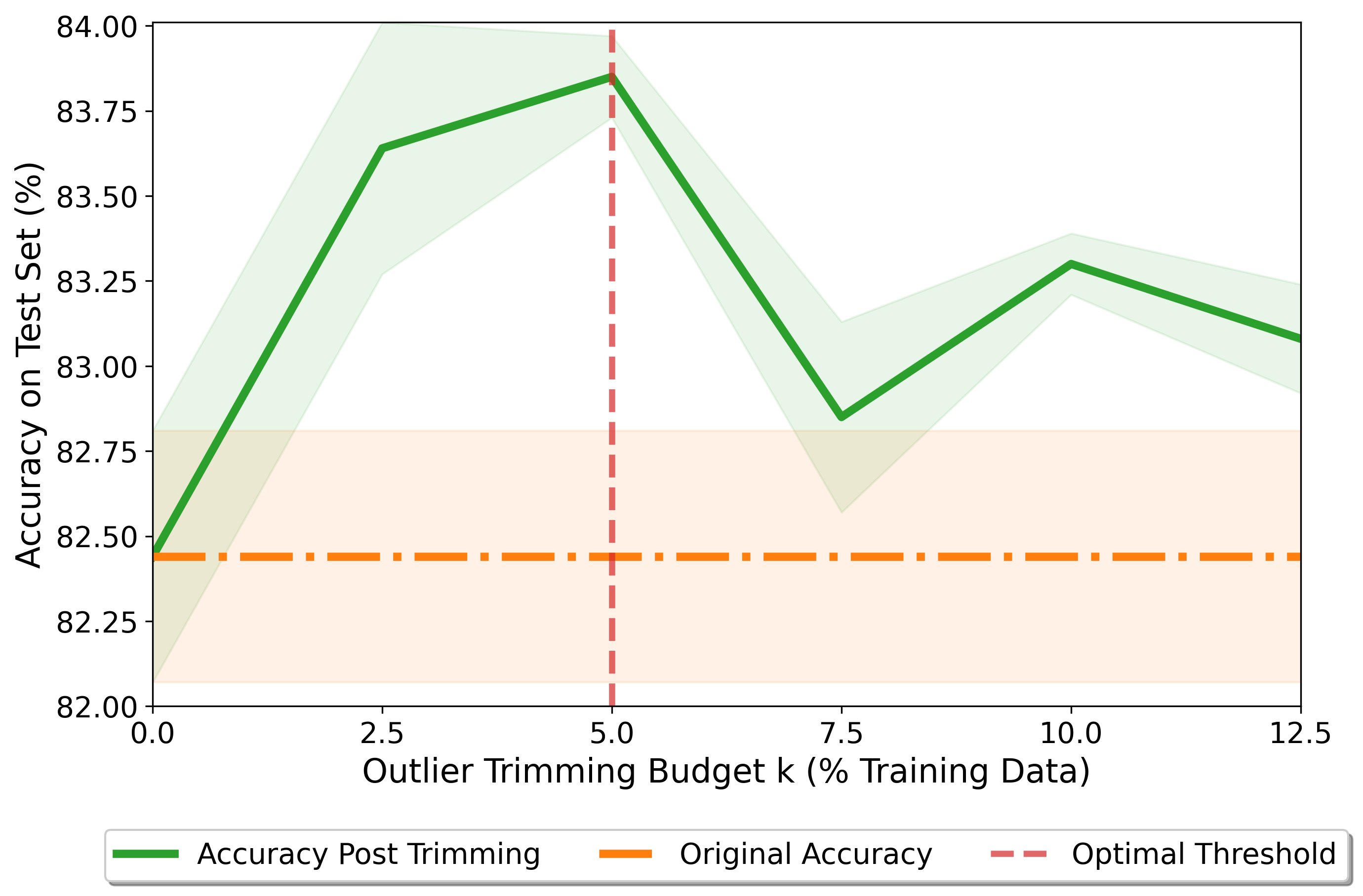
Figure 5: Test set performance measured for different outlier trimming budget values ($k$) as a percentage of the training data.

B.3 Experiments on Running Time and Computational Complexity

We now present running time experiments for outlier gradient analysis on both the CIFAR-10N and CIFAR-100N datasets compared to the other baselines compared in the paper in Table 5. It can be seen that outlier gradient analysis is computationally efficient and a fraction of the original running time of the model. Moreover, it is order of magnitudes faster than the other baselines. Thus, our outlier gradient analysis approach is computationally efficient as an option for trimming detrimental samples and improving model performance. We also provide analytical time complexity comparisons in Table 6. Although, it is important to note that in practice, outlier gradient analysis is much faster than the worst case time complexity, as can be seen in Table 5.

Table 5: Running time results for our outlier gradient analysis approaches and other baselines.

Method	Time Taken (seconds)
	CIFAR-10N (Aggregate)	CIFAR-10N (Random)	CIFAR-10N (Worst)	CIFAR-100N (Noisy100)
DataInf	3.89	3.99	4.01	15.22
LiSSA	23.75	23.25	23.26	115.19
Self-DataInf	5.29	5.51	5.5	12.1
Self-LiSSA	30.44	31.64	31.07	94.93
Outlier Gradient Analysis (L1)	0.54	0.54	0.74	10.3
Outlier Gradient Analysis (L2)	0.55	0.55	0.8	8.99
Outlier Gradient Analysis (iForest)	2.09	2.15	2.19	8.46

Table 6: Computational complexity of outlier gradient analysis methods and other baseline approaches ($n$ is #training samples, $v$ is #validation/test samples, $p$ is #model parameters, $m$ is #inputs for LLM and $o$ is #outputs for LLM).

Method	Type	Time Complexity
Exact (Eq 1)	Hessian-based	$\mathcal{O}(nv^{3})$
LiSSA Koh and Liang [2017]	Hessian-based	$\mathcal{O}(nvp)$
DataInf Kwon et al. [2024]	Hessian-based	$\mathcal{O}(nvp)$
Self-LiSSA Bejan et al. [2023]	Self-influence	$\mathcal{O}(np)$
Self-DataInf	Self-influence	$\mathcal{O}(np)$
SI LLM Baseline Grosse et al. [2023]	Self-influence	$\mathcal{O}(m^{2}o+p^{2}o)$
Gradient Tracing	Hessian-free	$\mathcal{O}(nvp)$
Ours (Outlier Gradient Analysis)	Hessian-free	$\mathcal{O}(np)$

B.4 Experiments with Varying Tree Estimators

We conduct further ablations for our iForest outlier gradient analysis approach. The main parameter (other than the trimming budget $k$, which we investigate in Appendix B.2) of iForest based outlier gradient analysis is the number of tree estimators being used. As a result, we vary the number of these estimators, and measure performance. We observe that test set performance on CIFAR-10N (Worst noise setting) for outlier gradient analysis remains stable across the board when number of estimators are varied, as can be seen in Table 7.

Table 7: Results on varying the number of tree estimators used in iForest outlier gradient analysis.

# Tree Estimators	Accuracy on Test Set (%)
25	83.70
50	84.38
75	83.71
100	83.72
125	83.66
150	83.97
175	83.84
200	83.42

B.5 Experiments on ImageNet

Although noisy label experiments have not been conducted on ImageNet Deng et al. [2009], we decided to undertake a simple experiment on a subset of ImageNet. We created a subset of ImageNet containing 50000 images (50 images from each of the 1000 classes) as the training set, and flip 40% of the corresponding image labels to create noisy labels (20 images from each class). The validation set is the same as ImageNet with 50000 images. We obtain results for performance on this set for a baseline ResNet-18 He et al. [2016] model, DataInf, Gradient Tracing, iForest based outlier gradient analysis, as well as simple L1-norm and L2-norm thresholding based outlier gradient analysis. The models are trained for 10 epochs. In this limited experimental setting, we obtain the following results in Table 8 and find that outlier gradient analysis methods achieve competitive performance to other methods while being highly computationally efficient.

Table 8: Results on ImageNet (top-3 performers based on both performance as well as time taken are in bold).

Method	Accuracy (%)	Time Taken (s)
Cross Entropy	49.15	-
Gradient Tracing	51.04	6.68e-4
DataInf	51.50	182.3
Outlier Gradient Analysis (iForest)	50.32	103.5
Outlier Gradient Analysis (L1)	51.48	44.81
Outlier Gradient Analysis (L2)	51.23	44.68

B.6 Experiments on ResNet-18 Architecture

We also provide results for ResNet-18 He et al. [2016] being used as the base model instead of the ResNet-34 model. The overall performance of the ResNet-18 model is lower than ResNet-34 for all datasets and noise settings since the ResNet-18 model has fewer residual connections than the ResNet-34 model. Moreover, it can be observed that outlier gradient analysis leads to improved performance post trimming, compared to the cross entropy baseline. Clearly, outlier gradient trimming is advantageous as a data selection strategy irrespective of the base model being used.

Table 9: Accuracy ± Standard Deviation results obtained for 5 runs on the CIFAR-10N and CIFAR-100N datasets for a ResNet-18 model trained via cross entropy as well performance post trimming using noisy label correction approaches and influence-based methods, including our proposed outlier gradient analysis.

Method	CIFAR-10N			CIFAR-100N
	Aggregate	Random	Worst	Noisy100
Cross Entropy	90.78 ± 0.12	89.01 ± 0.31	81.85 ± 0.45	57.22 ± 0.12
Outlier Gradient Trimming (Ours)	91.17 ± 0.14	89.91 ± 0.21	83.08 ± 0.26	60.58 ± 0.28

Appendix C Broader Impact and Limitations

Our work and proposed techniques aim to address issues that currently hinder the applicability of influence estimation in deep learning models. Enabling influence estimation for deep models allows practitioners to assess whether training samples are beneficial or detrimental to performance, and can make models more interpretable and performant. As we show through extensive experiments on multiple problem settings, our proposed outlier gradient analysis approach outperforms existing baselines and can augment model performance by trimming detrimental samples in a computationally efficient manner. As a result, our work paves the way for significant positive societal impact, especially with the increased adoption of larger and deeper neural networks such as LLMs. However, as with any work, there are limitations to our approaches that can be overcome in future work. For instance, it might be possible to derive specific outlier analysis algorithms that are computationally more efficient than iForest or norm thresholding, and significantly more performant. Another limitation that can be overcome is the further study and benchmarks for influence based analysis in LLMs– going beyond the datasets and approaches of [Kwon et al., 2024] we used in this work. Finally, influence approaches can also be studied for generation tasks in vision based models.

Appendix D Code and Reproducibility

We will provide our code, instructions, and implementation in an open-source repository shortly. The experiments were conducted on two separate Linux (Ubuntu 20.04.6 LTS) servers– the experiments of Sections 6 and 7 were conducted on NVIDIA GeForce RTX A6000 GPUs with 50GB VRAM running CUDA version 12.0 and all other experiments were conducted on a NVIDIA Tesla V100 with 32GB VRAM and CUDA version 11.4.

References

- Oala et al. (2023) Luis Oala, Manil Maskey, Lilith Bat-Leah, Alicia Parrish, Nezihe Merve Gürel, Tzu-Sheng Kuo, Yang Liu, Rotem Dror, Danilo Brajovic, Xiaozhe Yao, et al. Dmlr: Data-centric machine learning research–past, present and future. arXiv preprint arXiv:2311.13028, 2023.
- Zha et al. (2023) Daochen Zha, Zaid Pervaiz Bhat, Kwei-Herng Lai, Fan Yang, Zhimeng Jiang, Shaochen Zhong, and Xia Hu. Data-centric artificial intelligence: A survey. arXiv preprint arXiv:2303.10158, 2023.
- Chhabra et al. (2024) Anshuman Chhabra, Peizhao Li, Prasant Mohapatra, and Hongfu Liu. What Data Benefits My Classifier? Enhancing Model Performance and Interpretability through Influence-Based Data Selection. In International Conference on Learning Representations, 2024.
- Kwon et al. (2024) Yongchan Kwon, Eric Wu, Kevin Wu, and James Zou. DataInf: Efficiently Estimating Data Influence in LoRA-tuned LLMs and Diffusion Models. In International Conference on Learning Representations, 2024.
- Hammoudeh and Lowd (2022) Zayd Hammoudeh and Daniel Lowd. Training data influence analysis and estimation: A survey. arXiv preprint arXiv:2212.04612, 2022.
- Cook and Weisberg (1982) R Dennis Cook and Sanford Weisberg. Residuals and influence in regression. New York: Chapman and Hall, 1982.
- Ghorbani and Zou (2019) Amirata Ghorbani and James Zou. Data shapley: Equitable valuation of data for machine learning. In International Conference on Machine Learning, 2019.
- Jia et al. (2019) Ruoxi Jia, David Dao, Boxin Wang, Frances Ann Hubis, Nick Hynes, Nezihe Merve Gürel, Bo Li, Ce Zhang, Dawn Song, and Costas J Spanos. Towards efficient data valuation based on the shapley value. In International Conference on Artificial Intelligence and Statistics, 2019.
- Koh and Liang (2017) Pang Wei Koh and Percy Liang. Understanding black-box predictions via influence functions. In International Conference on Machine Learning, 2017.
- Basu et al. (2020a) Samyadeep Basu, Phil Pope, and Soheil Feizi. Influence Functions in Deep Learning Are Fragile. In International Conference on Learning Representations, 2020a.
- Bertsimas et al. (2016) Dimitris Bertsimas, Angela King, and Rahul Mazumder. Best subset selection via a modern optimization lens. The Annals of Statistics, 2016.
- Liu et al. (2019) Yinhan Liu, Myle Ott, Naman Goyal, Jingfei Du, Mandar Joshi, Danqi Chen, Omer Levy, Mike Lewis, Luke Zettlemoyer, and Veselin Stoyanov. Roberta: A robustly optimized bert pretraining approach. arXiv preprint arXiv:1907.11692, 2019.
- Kwon and Zou (2022) Yongchan Kwon and James Zou. Beta Shapley: a unified and noise-reduced data valuation framework for machine learning. In International Conference on Artificial Intelligence and Statistics, 2022.
- Jia et al. (2018) Ruoxi Jia, David Dao, Boxin Wang, Frances Ann Hubis, Nezihe Merve Gurel, Bo Li, Ce Zhang, Costas Spanos, and Dawn Song. Efficient task specific data valuation for nearest neighbor algorithms. Proceedings of the VLDB Endowment, 2018.
- Agarwal et al. (2017) Naman Agarwal, Brian Bullins, and Elad Hazan. Second-order stochastic optimization for machine learning in linear time. The Journal of Machine Learning Research, 2017.
- Yeh et al. (2018) Chih-Kuan Yeh, Joon Kim, Ian En-Hsu Yen, and Pradeep K Ravikumar. Representer point selection for explaining deep neural networks. Advances in Neural Information Processing Systems, 2018.
- Chen et al. (2021) Yuanyuan Chen, Boyang Li, Han Yu, Pengcheng Wu, and Chunyan Miao. Hydra: Hypergradient data relevance analysis for interpreting deep neural networks. In AAAI Conference on Artificial Intelligence, 2021.
- Schioppa et al. (2022) Andrea Schioppa, Polina Zablotskaia, David Vilar, and Artem Sokolov. Scaling up influence functions. In AAAI Conference on Artificial Intelligence, 2022.
- Feldman and Zhang (2020) Vitaly Feldman and Chiyuan Zhang. What neural networks memorize and why: Discovering the long tail via influence estimation. Advances in Neural Information Processing Systems, 2020.
- Pruthi et al. (2020) Garima Pruthi, Frederick Liu, Satyen Kale, and Mukund Sundararajan. Estimating training data influence by tracing gradient descent. Advances in Neural Information Processing Systems, 2020.
- Charpiat et al. (2019) Guillaume Charpiat, Nicolas Girard, Loris Felardos, and Yuliya Tarabalka. Input similarity from the neural network perspective. Advances in Neural Information Processing Systems, 2019.
- Kong et al. (2021) Shuming Kong, Yanyan Shen, and Linpeng Huang. Resolving training biases via influence-based data relabeling. In International Conference on Learning Representations, 2021.
- Grosse et al. (2023) Roger Grosse, Juhan Bae, Cem Anil, Nelson Elhage, Alex Tamkin, Amirhossein Tajdini, Benoit Steiner, Dustin Li, Esin Durmus, Ethan Perez, et al. Studying large language model generalization with influence functions. arXiv preprint arXiv:2308.03296, 2023.
- Schioppa et al. (2024) Andrea Schioppa, Katja Filippova, Ivan Titov, and Polina Zablotskaia. Theoretical and practical perspectives on what influence functions do. Advances in Neural Information Processing Systems, 2024.
- Bejan et al. (2023) Irina Bejan, Artem Sokolov, and Katja Filippova. Make every example count: On the stability and utility of self-influence for learning from noisy nlp datasets. In Proceedings of the 2023 Conference on Empirical Methods in Natural Language Processing, 2023.
- Thakkar et al. (2023) Megh Thakkar, Tolga Bolukbasi, Sriram Ganapathy, Shikhar Vashishth, Sarath Chandar, and Partha Talukdar. Self-influence guided data reweighting for language model pre-training. In Proceedings of the 2023 Conference on Empirical Methods in Natural Language Processing, 2023.
- Ilyas et al. (2022) Andrew Ilyas, Sung Min Park, Logan Engstrom, Guillaume Leclerc, and Aleksander Madry. Datamodels: Predicting predictions from training data. arXiv preprint arXiv:2202.00622, 2022.
- Jain et al. (2023) Eeshaan Jain, Tushar Nandy, Gaurav Aggarwal, Ashish V. Tendulkar, Rishabh K Iyer, and Abir De. Efficient Data Subset Selection to Generalize Training Across Models: Transductive and Inductive Networks. In Advances in Neural Information Processing Systems, 2023.
- Paul et al. (2021) Mansheej Paul, Surya Ganguli, and Gintare Karolina Dziugaite. Deep learning on a data diet: Finding important examples early in training. In Advances in Neural Information Processing Systems, 2021.
- Killamsetty et al. (2021) Krishnateja Killamsetty, Xujiang Zhao, Feng Chen, and Rishabh Iyer. Retrieve: Coreset selection for efficient and robust semi-supervised learning. Advances in Neural Information Processing Systems, 2021.
- Tan et al. (2024) Haoru Tan, Sitong Wu, Fei Du, Yukang Chen, Zhibin Wang, Fan Wang, and Xiaojuan Qi. Data pruning via moving-one-sample-out. Advances in Neural Information Processing Systems, 36, 2024.
- Yang et al. (2022) Shuo Yang, Zeke Xie, Hanyu Peng, Min Xu, Mingming Sun, and Ping Li. Dataset pruning: Reducing training data by examining generalization influence. In The Eleventh International Conference on Learning Representations, 2022.
- Lyu et al. (2023) Hyeonsu Lyu, Jonggyu Jang, Sehyun Ryu, and Hyun Jong Yang. Deeper understanding of black-box predictions via generalized influence functions. arXiv preprint arXiv:2312.05586, 2023.
- Chhabra et al. (2022) Anshuman Chhabra, Adish Singla, and Prasant Mohapatra. Fair clustering using antidote data. In Algorithmic Fairness through the Lens of Causality and Robustness Workshop, 2022.
- Li et al. (2023) Peizhao Li, Ethan Xia, and Hongfu Liu. Learning antidote data to individual unfairness. In International Conference on Machine Learning, 2023.
- Hall (1999) Mark A Hall. Correlation-based feature selection for machine learning. PhD thesis, The University of Waikato, 1999.
- Cai et al. (2018) Jie Cai, Jiawei Luo, Shulin Wang, and Sheng Yang. Feature selection in machine learning: A new perspective. Neurocomputing, 2018.
- Cohn et al. (1996) David A Cohn, Zoubin Ghahramani, and Michael I Jordan. Active learning with statistical models. Journal of Artificial Intelligence Research, 1996.
- Liu et al. (2021) Zhuoming Liu, Hao Ding, Huaping Zhong, Weijia Li, Jifeng Dai, and Conghui He. Influence selection for active learning. In IEEE/CVF International Conference on Computer Vision, 2021.
- Nguyen et al. (2022) Vu-Linh Nguyen, Mohammad Hossein Shaker, and Eyke Hüllermeier. How to measure uncertainty in uncertainty sampling for active learning. Machine Learning, 2022.
- Wei et al. (2015) Kai Wei, Rishabh Iyer, and Jeff Bilmes. Submodularity in data subset selection and active learning. In International Conference on Machine Learning, 2015.
- Solans et al. (2021) David Solans, Battista Biggio, and Carlos Castillo. Poisoning attacks on algorithmic fairness. In Machine Learning and Knowledge Discovery in Databases: European Conference, 2021.
- Mehrabi et al. (2021) Ninareh Mehrabi, Muhammad Naveed, Fred Morstatter, and Aram Galstyan. Exacerbating algorithmic bias through fairness attacks. In AAAI Conference on Artificial Intelligence, 2021.
- Chhabra et al. (2023) Anshuman Chhabra, Peizhao Li, Prasant Mohapatra, and Hongfu Liu. Robust fair clustering: A novel fairness attack and defense framework. In International Conference on Learning Representations, 2023.
- Dai and Gifford (2023) Zheng Dai and David K Gifford. Training data attribution for diffusion models. arXiv preprint arXiv:2306.02174, 2023.
- Hampel (1974) Frank R Hampel. The influence curve and its role in robust estimation. Journal of the american statistical association, 1974.
- Martin and Yohai (1986) R Douglas Martin and Victor J Yohai. Influence functionals for time series. The Annals of Statistics, 1986.
- Han et al. (2020) Xiaochuang Han, Byron C Wallace, and Yulia Tsvetkov. Explaining black box predictions and unveiling data artifacts through influence functions. In Annual Meeting of the Association for Computational Linguistics, 2020.
- Basu et al. (2020b) Samyadeep Basu, Xuchen You, and Soheil Feizi. On second-order group influence functions for black-box predictions. In International Conference on Machine Learning, 2020b.
- Alaa and Van Der Schaar (2020) Ahmed Alaa and Mihaela Van Der Schaar. Discriminative jackknife: Quantifying uncertainty in deep learning via higher-order influence functions. In International Conference on Machine Learning, 2020.
- Liu et al. (2008) Fei Tony Liu, Kai Ming Ting, and Zhi-Hua Zhou. Isolation forest. In IEEE International Conference on Data Mining, 2008.
- Knorr et al. (2000) Edwin M Knorr, Raymond T Ng, and Vladimir Tucakov. Distance-based outliers: algorithms and applications. The VLDB Journal, 2000.
- Northcutt et al. (2021) Curtis Northcutt, Lu Jiang, and Isaac Chuang. Confident learning: Estimating uncertainty in dataset labels. Journal of Artificial Intelligence Research, 2021.
- Müller and Markert (2019) Nicolas M Müller and Karla Markert. Identifying mislabeled instances in classification datasets. In International Joint Conference on Neural Networks, 2019.
- Kuan and Mueller (2022) Johnson Kuan and Jonas Mueller. Model-agnostic label quality scoring to detect real-world label errors. In ICML DataPerf Workshop, 2022.
- Wei et al. (2022) Jiaheng Wei, Zhaowei Zhu, Hao Cheng, Tongliang Liu, Gang Niu, and Yang Liu. Learning with noisy labels revisited: A study using real-world human annotations. In International Conference on Learning Representations, 2022.
- Krizhevsky et al. (2009) Alex Krizhevsky, Geoffrey Hinton, et al. Learning multiple layers of features from tiny images. University of Toronto, 2009.
- He et al. (2016) Kaiming He, Xiangyu Zhang, Shaoqing Ren, and Jian Sun. Deep residual learning for image recognition. In IEEE/CVF Conference on Computer Vision and Pattern Recognition, 2016.
- Deng et al. (2009) Jia Deng, Wei Dong, Richard Socher, Li-Jia Li, Kai Li, and Li Fei-Fei. Imagenet: A large-scale hierarchical image database. In 2009 IEEE conference on computer vision and pattern recognition, pages 248–255. Ieee, 2009.
- Wang et al. (2018) Alex Wang, Amanpreet Singh, Julian Michael, Felix Hill, Omer Levy, and Samuel Bowman. GLUE: A Multi-Task Benchmark and Analysis Platform for Natural Language Understanding. arXiv preprint arXiv:1804.07461., 2018.
- Hu et al. (2022) Edward J Hu, yelong shen, Phillip Wallis, Zeyuan Allen-Zhu, Yuanzhi Li, Shean Wang, Lu Wang, and Weizhu Chen. LoRA: Low-Rank Adaptation of Large Language Models. In International Conference on Learning Representations, 2022.
- Socher et al. (2013) Richard Socher, Alex Perelygin, Jean Wu, Jason Chuang, Christopher D Manning, Andrew Y Ng, and Christopher Potts. Recursive deep models for semantic compositionality over a sentiment treebank. In Proceedings of the 2013 conference on empirical methods in natural language processing, pages 1631–1642, 2013.
- Dolan and Brockett (2005) Bill Dolan and Chris Brockett. Automatically constructing a corpus of sentential paraphrases. In Third International Workshop on Paraphrasing (IWP2005), 2005.
- Li et al. (2006) Ping Li, Trevor J Hastie, and Kenneth W Church. Very sparse random projections. In Proceedings of the 12th ACM SIGKDD international conference on Knowledge discovery and data mining, pages 287–296, 2006.