definitionDefinition[section] \newdefinitionremark[definition]Remark \newproofproofProof \newproofpotProof of Theorem LABEL:thm
[1]
1]organization=Centro de Bioinformática Médica, Universidade Federal de São Paulo, addressline=Edifício de Pesquisas 2, city=São Paulo, postcode=04039-032, state=SP, country=Brazil
[cor1]Corresponding author
2]organization=Department of Mathematics, The Ohio State University, addressline=231 W 18th Ave, city=Columbus, postcode=43210, state=OH, country=USA
3]organization=Mathematics Institute, University of Warwick, addressline=Zeeman Building, city=Coventry, citysep=, postcode=CV4 7AL, country=UK
Homeostasis in Input-Output Networks:
Structure, Classification and Applications
Abstract
Homeostasis is concerned with regulatory mechanisms, present in biological systems, where some specific variable is kept close to a set value as some external disturbance affects the system. Many biological systems, from gene networks to signaling pathways to whole tissue/organism physiology, exhibit homeostatic mechanisms. In all these cases there are homeostatic regions where the variable is relatively to insensitive external stimulus, flanked by regions where it is sensitive. Mathematically, the notion of homeostasis can be formalized in terms of an input-output function that maps the parameter representing the external disturbance to the output variable that must be kept within a fairly narrow range. This observation inspired the introduction of the notion of infinitesimal homeostasis, namely, the derivative of the input-output function is zero at an isolated point. This point of view allows for the application of methods from singularity theory to characterize infinitesimal homeostasis points (i.e. critical points of the input-output function). In this paper we review the infinitesimal approach to the study of homeostasis in input-output networks. An input-output network is a network with two distinguished nodes ‘input’ and ‘output’, and the dynamics of the network determines the corresponding input-output function of the system. This class of dynamical systems provides an appropriate framework to study homeostasis and several important biological systems can be formulated in this context. Moreover, this approach, coupled to graph-theoretic ideas from combinatorial matrix theory, provides a systematic way for classifying different types of homeostasis (homeostatic mechanisms) in input-output networks, in terms of the network topology. In turn, this leads to new mathematical concepts, such as, homeostasis subnetworks, homeostasis patterns, homeostasis mode interaction. We illustrate the usefulness of this theory with several biological examples: biochemical networks, chemical reaction networks (CRN), gene regulatory networks (GRN), Intracellular metal ion regulation and so on.
keywords:
Infinitesimal Homeostasis \sepInput-Output Networks \sepPerfect Adaptation1 Introduction
The idea of homeostasis has its roots in the work of the French physiologist Claude Bernard [17] who observed a kind of regulation in the ‘milieu intérieur’ (internal environment) of human organs such as the liver and pancreas. The term ’homeostasis’, coined by the American physiologist Walter Cannon in 1926 [24, 25], derives from the Greek language and refers to a capacity of maintaining similar stasis. In this context, ‘homeostasis’ refers to certain regulatory mechanisms by which a feature is maintained at a steady state despite disturbances caused by changes in the environment. At the scale of a whole organism, homeostasis manifests itself in many forms: body temperature, blood sugar level, concentration of ions in body fluids with changes in the external environment.
More recently, the study of homeostasis in biological systems through mathematical models has gained prominence. For example, the extensive work of Nijhout, Reed, Best and collaborators [107, 18, 106, 105, 104] consider biochemical networks associated with metabolic signaling pathways. Further examples include regulation of cell number and size [87], control of sleep [135], and expression level regulation in housekeeping genes [7].
In order to mathematically model ‘homeostasis’ is necessary to have a framework where a precise definition can be given. The simplest mathematical setup, very often used to model biological phenomena, is the theory of ordinary differential equations. In this setting ‘homeostasis’ can be interpreted in two mathematically distinct ways. One boils down to the existence of a ‘globally stable equilibrium’. Here, changes in the environment are considered to be perturbations of initial conditions [128]. A stronger (and, in our view, more appropriate) usage works with a parametrized family of differential equations, with a corresponding family of stable equilibria. Now ‘homeostasis’ means that some quantity defined through this equilibrium changes by a relatively small amount when the parameter varies by a much larger amount. Homeostasis does not imply that the whole system remains invariant with change in external variables. In fact, changes in external variables can cause changes in certain internal variables, while other internal variables remain almost unchanged.
A precise definition of homeostasis can be give as follows. Consider system of ODEs depending on an input parameter , which varies over a range of external stimuli. Suppose there is a family of equilibrium points and an observable , such that the input-output function is well-defined on the range of . In this situation, we say that the system exhibits homeostasis if, under variation of the input parameter , the input-output function remains approximately constant over the interval of external stimuli (see section 2). Golubitsky and Stewart [54] observe that homeostasis on some neighborhood of a specific value follows from infinitesimal homeostasis, where and ′ indicates differentiation with respect to . This observation is essentially the well-known idea that the value of a function changes most slowly near a stationary (or critical) point.
Infinitesimal homeostasis is a sufficient condition for homeostasis over some interval of parameters, but it is not a necessary condition. A function can vary slowly without having a stationary point. In applications, the quantity that experiences homeostasis, represented by the observable can be a function of several internal variables, such as a sum of concentrations, or the period of an oscillation (see subsection 4.4).
There are other variations on the formulation of homeostasis. Control-theoretic models of homeostasis often require perfect homeostasis, also known as perfect adaptation, in which the input-output function is exactly constant over the parameter range [80, 81, 47]. The requirement of perfect homeostasis is very strong, demanding that the model equations have a somewhat restricted functional form [10].
Another important idea of [54] is to take advantage of fact that infinitesimal homeostasis is suitable for analysis using methods from singularity theory (see subsection 2.2). A motivational example for the use of singularity theory to analyze homeostasis is the regulation of the output ‘body temperature’ in an opossum, when the input ‘environmental temperature’ varies [101]. In [57, Figs. 1–2] the graphs of body temperature against environmental temperature are approximately linear, with nonzero slope, when is either small or large, while in between is a broad flat region, where homeostasis occurs. This general shape is called a ‘chair’ by Nijhout and Reed [106] (see also [103, 107]) and suggest that there is a chair in the body temperature data of opossums [101] given by such a piecewise linear function [103, Fig. 1]. Golubitsky and Stewart [54] take a singularity-theoretic point of view and suggest that chairs are better described locally by a homogeneous cubic function (that is, like ) rather than by the previous piecewise linear description. Based on this suggestion, [54] goes on to show that the singularities of input-output functions are described by Elementary Catastrophe Theory [126, 127, 142].
The last contribution of [54] is that homeostasis can be thought of as a network concept. This is motivated by the abundance of networks in biology, specially connected to ODE modeling, see e.g. [103, 115, 46]. In fact, almost all ODE models in biology come together with a ‘wiring diagram’, or a network, describing the interactions among the elements in the model. The recently published book [56] gives an exposition of a formal framework for studying networks of coupled ODEs, that have been developed the authors and collaborators in the past decade. More precisely, a network of coupled ODEs is determined by directed graph whose nodes and edges are classified into types. Nodes, or cells, represent the variables of a component ODE. Edges, or arrows, between nodes represent couplings from the tail node to the head node. Nodes of the same type have the same phase spaces (up to a canonical identification); edges of the same type represent identical couplings.
In the setting of network coupled ODEs there is a preferable class of observables, namely the output of the node variables (coordinate functions). Network systems are distinguished from large systems by the ability to keep track of the output from each node individually. Now homeostasis can be naturally defined as the fact that the output of a node variable (the ‘output node’) is held approximately constant as other variables (other nodes) vary (perhaps wildly) under variation of an input parameter that affects another node (the ‘input node’). Placing homeostasis in the general context of network dynamics leads naturally to the methods reviewed here.
A special kind of network of coupled ODE, with two distinguished nodes (one input node and one output node) is called an input-output network. It was introduced in [58] in their study of homeostasis on -node networks. Wang et al. [134] extended the notion of input-output network to arbitrary large networks and developed a combinatorial theory for the classification of ‘homeostasis types’ in such networks. A homeostasis type is essentially a ‘combinatorial mechanism’ that causes homeostasis in the full network and is represented by specific subnetworks, called homeostasis subnetworks. The homeostasis subnetworks can be subdivided into to classes called structural and appendage.
The motivation for the term structural homeostasis comes from [115], where the authors identify the feedforward loop as one of the homeostastic motifs in -node biochemical networks, that is, a generalized ‘feedforward loop’ The intuition behind the term appendage homeostasis is that homeostasis is generated by a cycle of regulatory nodes, that is, a generalized ‘feedback loop’. The structural and appendage classes are abstract generalizations of the usual ‘feedforward’ and ‘feedback’ mechanisms. A striking outcome the approach of [134] is that they do not specify any homeostasis generating mechanisms at the outset and they find a posteriori that there are essentially only the two types of homeostasis generating mechanisms: generalized feedback and generalized feedforward.
In Duncan et al. [40] the combinatorial formalism of [134] id further refined to allow one to determine, for each homeostasis subnetwork, which nodes are (and are not) going to be simultaneously homeostatic (besides the designated output node) when that particular homeostasis subnetwrok is the ‘homeostasis trigger’, i.e. the one that causes homeostasis in the network. These collections of simultaneous homeostatic nodes are called homeostasis patterns. The general picture that emerges from all these results is the following: the homeostasis subnetworks and the homeostasis patterns of network correspond uniquely to each other.
2 Structure
In this section we give the basic definition of homeostasis in a parametrized system of ordinary differential equations. We start with a very general definition that will be specialized to more ‘concrete’ situations throughout the paper.
2.1 A Dynamical Formalism for Homeostasis
Golubitsky and Stewart [54, 55] proposed a mathematical framework for the study of homeostasis based on dynamical systems theory (see [57] and the book [56]).
In this framework one considers a system of differential equations
| (2.1) |
with state variable and input parameters representing the external input to the system.
Suppose that is a linearly stable equilibrium of (2.1). By the implicit function theorem, there is a function defined in a neighborhood of such that and .
A smooth function is called an observable. Define the input-output function associated to and as . The input-output function allows one to formulate several definitions that capture the notion of homeostasis (see [89, 4, 125, 54, 55]).
Definition 2.1.
Let be an input-output function. We say that exhibits
-
[(a)]
-
1.
Perfect Homeostasis on an open set if
(2.2) That is, is constant on .
-
2.
Near-perfect Homeostasis relative to a set point if, for fixed ,
(2.3) That is, stays within the range over .
-
3.
Infinitesimal Homeostasis at the point if
(2.4) That is, is a critical point of .
It is clear that perfect homeostasis implies near-perfect homeostasis, but the converse does not hold. Inspired by Nijhout, Reed, Best et al. [107, 18, 103], Golubitsky and Stewart [54, 55] introduced the notion of infinitesimal homeostasis which is intermediate between perfect and near-perfect homeostasis. It is obvious that perfect homeostasis implies infinitesimal homeostasis. On the other hand, it follows from Taylor’s theorem that infinitesimal homeostasis implies near-perfect homeostasis in a neighborhood of (see [56] for details). It is easy to see that the converse to both implications is not generally valid (see Reed et al. [115]).
The geometric interpretation of infinitesimal homeostasis is that, if is a critical point of the input-output function, then differs from in a manner that depends quadratically (or to higher order) on . This makes the graph of flatter than any growth rate with a nonzero linear term.
Definition 2.1 is very general in the sense that it allows for an arbitrary number of input parameters and and arbitrary (smooth) function of state variables as the output. In the engineering literature, a system of inputs and outputs can be described as one of four types: SISO (single input, single output), SIMO (single input, multiple output), MISO (multiple input, single output), or MIMO (multiple input, multiple output). By this terminology, Definition 2.1 describes MIMO systems. However, as in bifurcation theory, the most important situation is when a single scalar input parameter is considered at a time. Moreover, as we will define latter there is a natural class of dynamical systems, called network dynamical systems or coupled cell systems, that comes with a distinguished set of observables [56]. By adjusting the notion of homeostasis with a single input parameter to work in the class of network dynamical systems we obtain a very general description of SISO systems, called input-output networks. Remarkably, it is in this class of systems that we can obtain the most complete theory of homeostasis (see Subsection 2.3).
Nevertheless, we can still say something in the most general setting. We can use implicit differentiation and the cofactor formula for the inverse of a matrix to write a formula for . Let us denote the Jacobian matrix of at the equilibrium (we will omit the ~ over from now on) by
The partial derivatives of with respect to are denoted by and the partial derivatives with respect to are denoted by . Let denote the vector of partial derivatives of with respect to , that is, .
Lemma 2.2.
Let be an input-output function associated to a system of differential equations (2.1). The gradient of with respect to the multiple input is given by
| (2.5) |
where is the adjugate matrix or classical adjoint of (defined as the transpose of the cofactor matrix of ). In particular, is an infinitesimal homeostasis point of if and only if
| (2.6) |
Proof 2.3.
The gradient of is
| (2.7) |
The partial derivative of with respect to (for each ) is
| (2.8) |
where is the partial derivative of with respect to . Implicit differentiation of the equation , with respect to , yields the linear system
| (2.9) |
From (2.9) and the fact that is assumed to be a linearly stable equilibrium, for all , and hence over , it follows that
| (2.10) |
Therefore, substituting (2.10) into (2.8) and then into (2.7) we obtain (2.5). ∎
Lemma 2.2 allows us to draw some general remarks about the function . The first observation is that the term is a multivariate polynomial in the partial derivatives and , linear in . Hence, the defining equations for homeostasis (2.6) are polynomial functions in the partial derivatives , and , linear in both and . This will become manifest in the several examples discussed in the paper.
The second observation is that there are two ‘trivial’ ways in which homeostasis can occur: (i) by the existence of a critical point of , that is, at , and (ii) the simultaneous vanishing of all at . The first case depends on the choice of the observable and it indeed occurs in some applications, for instance [107] (see Example 2.4 below). The second case is a highly non-generic situation which essentially says that the system is homeostatic “at the input source”. Henceforth, unless stated otherwise, we always assume the following genericity condition: the derivative of the vector field with respect to the input parameters generically satisfies
| (2.11) |
The third observation is that the formula (2.5) is valid as long as the equilibrium is linearly stable, since at . Moreover, at some if and only if is a steady-state bifurcation point. Therefore, the input-output function is non-differentiable at the steady-state bifurcation points of . Although it may be continuously extended beyond those points and become differentiable again.
The final observation is concerned with the fact that, very often, model equations depend on several parameters (besides the input parameters). Because of this dependence the equilibrium family and input-output function may also depend on some of these parameters (generically, they depend on all of them), but they are suppressed from most the time.
More precisely, if we write the vector field in (2.1) as , where is the vector of all scalar parameters that appear in the definition of then the implicit function theorem applied to a point gives the function defined in a neighborhood of such that and . Therefore, the input-output function can be written as and infinitesimal homeostasis may depend on a fixed . That is, infinitesimal homeostasis occurs at only when .
It is here that notion of infinitesimal homeostasis places the study of homeostasis in the context of singularity theory. For instance, the dependence on the parameters for the occurrence of infinitesimal homeostasis is related to higher degeneracy conditions, in addition to (2.4), which leads to distinct ‘forms’ of infinitesimal homeostasis.
For example, let us consider the single parameter case . We say that exhibits simple homeostasis if
| (2.12) |
In this case, is called a Morse singularity (or a nondegenerate critical point) and it is persistent under any small perturbation of (see subsection 2.2). In fact, a Morse singularity is persistent under any small perturbation of in the space of smooth functions (with the appropriate topology) [51]. We say that exhibits chair homeostasis if
| (2.13) |
In this case, there is at least one parameter (or a combination of several components of ) that should be fixed together with to have infinitesimal homeostasis. However, as we will see below, singularity theory implies that small perturbations of (that is, variation of the suppressed parameters) change the ‘almost flat region’ only slightly. Following Nijhout et al. [103] we define a plateau as a region of over which is approximately constant. In other words, the infinitesimal homeostasis points are not persistent, but the family of functions have a plateau for all in a neighborhood of (see Definition 2.10 in subsection 2.2).
The observation that an unstable structure ‘determines’ (unfolds) all the neighboring stable behaviors goes back to René Thom’s notion of a singularity as an organizing center [127]. Even though the singularity itself is unstable under perturbation, it ‘organizes’ all its small perturbations into the universal unfolding. Unlike the singularity, the universal unfolding is structurally stable and thus contains all the possible persistent behaviors, as well as the number of parameters to (qualitatively) model all those behaviors.
This is important in applications because it may be very difficult to calculate exactly the values of where infinitesimal homeostasis occurs and then one must resort to numerical methods. It is possible to compute parts of the graph of input-output functions and find the plateau using numerical methods for continuation of equilibrium points, such as Auto from XPPAut [44] (for example, see Figure 7 in subsection 2.4 and Figure 25 in subsection 4.3).
Finally, we should mention that there is another notion of ‘robustness’ often referred in the control theoretic literature, see [4, 125, 10, 9] for example. This notion is closely related to other concepts such as structural identifiability [98, 99, 59, 60, 20] and dynamical compensation [77, 124, 132].
2.1.1 Examples of Homeostasis
Here we present some examples of input-output functions associated to biological models.
Example 2.4 (Folate Cycle).
Nijhout et al. [107] developed a model for the folate cycle based on standard biochemical kinetics and used the model to provide new insights into several different mechanisms of folate homeostasis. Their model is described by 6 ODEs for the concentrations of the following substrates [107, Eqs. 4–9]: (1) tetrahydrofolate (THF), (2) 5-methyltetrahydrofolate (5mTHF), (3) dihydrofolate (DHF), (4) 5,10-methylenetetrahydrofolate (5,10-CH2-THF), (5) 5,10-methenyltetrahydro-folate (5,10-CH=THF) and (6) 10-formyltetrahydrofolate (10f-THF). The coupling structure of the model is represented by a diagram containing the 6 substrates and additional 12 enzymes [107, Fig. 1]. In the model, folate enters and leaves the cell as 5mTHF as indicated by the presence of the input parameter in the corresponding differential equation Here, and are the rates at which 5mTHF enters and leaves the cell, respectively. The authors consider observables of the form representing the velocity of a reaction associated to ENZYME, called ‘fluxes’ [107, Tab. III], in terms of substrates. The smooth functions are given by certain expressions involving Michaelis-Menten functions [107, Eqs. 1–3]. The plots of the fluxes as functions of the input parameter were numerically computed and homeostasis is shown by the fact that velocities do not decline substantially until total folate is close to [107, Figs. 4–6]. It can be checked that the functions have a critical point completely determined by the kinetic parameters entering its definition.
Example 2.5 (Kidney Flow).
Sgouralis and Layton [119] show by using a mathematical model how well the effect of the myogenic mechanism affects the afferent arteriole flow rate (output) in response to pressure variation (input). The myogenic response in the smooth muscle enables nephrons to regulate the flow in afferent arterioles for a wide range of pressure values The solid curves in [119, Fig. 4] (see also [103, Fig. 6]) shows the percentage change at steady state in their model as the pressure in the afferent arteriole is varied from to . The flow rate is remarkably stable between and . Below the flow drops quickly and above the flow begins to increase substantially giving the same chair-shaped curve that we have seen in the Introduction. The dashed curves shows what the flow rate would be if the myogenic response were turned off and the walls of the arteriole responded passively.
Example 2.6 (Glycolysis Pathway).
Mulukutla et al. [102] use a mathematical model based on reported mechanisms for the allosteric regulations of the enzymes in the flux of glycolysis. They show that glycolysis exhibits multiple steady state behavior segregating glucose metabolism into high flux and low flux states. Here, the input parameter is the glucose consumption and the output variable is the specific lactate production. In [102, Fig. 3] the authors show a phenomenon of bistability of homeostasis in cultured HeLa cells (see also [41, Fig. 4]). The data suggests the existence of two homeostasis points on the lower branch: one which is apparent in the figure, and another which we would expect to see if it were extended further. The similar glucose consumption rates of both types of cells in very high and very low glucose environments indicate two switches on the border of the plateaus. The homeostasis points and the bistable behavior are suggestive of the behavior depicted [102, Fig. 2] obtained by simulation of the model equations. Duncan and Golubitsky [41, Fig. 3] propose a mechanism combining homeostasis and bifurcation that qualitatively reproduces the bistability observed in [102].
Example 2.7 (Extracellular Dopamine).
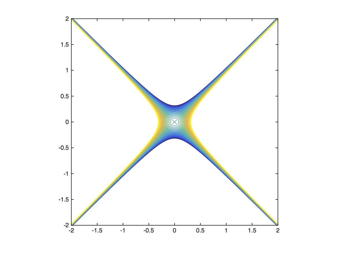
Best et al. [18, 103] propose a biological network to study homeostasis of extracellular dopamine (eDA) in response to variation in the activities of the enzyme tyrosine hydroxylase (TH) and the dopamine transporters (DAT). Hence, in this model we have two input parameters (eDA,TH) and one output variable DAT. The authors derive a differential equation model for the biochemical network [18, Fig. 1]. In [103] the authors fix reasonable values for all parameters in the model with the exception of the concentrations of TH and DAT. In [103, Fig. 8] the authors show the equilibrium value of eDA as a function of TH and DAT in their model. The white dots indicate the predicted eDA values for the observationally determined values of TH and DAT in the wild-type genotype (large white disk) and the polymorphisms observed in human populations (small white disks). These polymorphisms raise or lower the activity of TH and lower the activity of the DAT as indicated in [103, Tab. 1]. This result is scientifically important because almost all of these genetic polymorphisms (white disks) lie on the plateau and that indicates homeostasis of eDA. Presumably, this is because polymorphisms that would result in large changes in eDA are deleterious and would, therefore, be removed from the population. Thus, although the polymorphisms have large effects on the activities of TH and DAT, they have only a very small effect on the phenotypic variable eDA, and thus can be considered to be cryptic genetic variation. Note that the plateau contains a line from left to right at about eDA . In this respect, the surface graph in [103, Fig. 8] appears to resemble that of a non-singular perturbed hyperbolic umbilic (see Table 1) and Figure 2. See also the level contours of the hyperbolic umbilic in Figure 2. This figure shows that the hyperbolic umbilic is the only low-codimension singularity that contains a single line in its zero set, see [55] for more details.
2.2 Singularity Theory of Input-Output Functions: Elementary Catastrophe Theory
As discussed in the Introduction, Nijhout et al. [103] observe that homeostasis appears in many applications through the notion of a chair. Golubitsky and Stewart [55] observed that a chair can be thought of as a singularity of a scalar input-output function, one where ‘looks like’ a homogeneous cubic, e.g. . More precisely, the mathematics of singularity theory [112, 50] replaces ‘looks like’ by ‘up to a change of coordinates.’
Definition 2.8.
Definition 2.9.
Two smooth functions are right equivalent on a neighborhood of if
where is an invertible change of coordinates, or simply a diffeomorphism, on a neighborhood of and is a constant.
The simplest classification theorem of singularity theory states that is right equivalent to on a neighborhood of a singularity if and only if the singularity is nondegenerate. This is the content of the classical Morse Lemma. Geometrically, this says that the graph of ‘looks like’ a quadratic function near a nondegenerate singularity. Now, the the main goal of singularity theory is the study of degenerate singularities.
The transformations of the input-output map given in Definition 2.9 are just the standard change of coordinates in elementary catastrophe theory [50, 112, 142]. In [54, 55] it is shown that a special class of transformations on the vector field induces the class of right equivalences on the input-output functions. Although their proof is formulated for a special class of observables (the projections onto the coordinate variables) the use of right equivalence is completely justified. The proof that the action of the diffeomorphism on the vector field induces the correct action on the input-output function works in the general setting and the addition of the constant is justified because we are looking for plateaus on which is approximately constant but not specifically what that constant is.
Now we can therefore use standard results from elementary catastrophe theory to find normal forms and universal unfoldings of , as we now explain. Informally, the codimension of a singularity is the number of conditions on derivatives that determine it. This is also the minimum number of extra variables required to specify all small perturbations of the singularity, up to changes of coordinates. These perturbations can be organized into a family of maps called the universal unfolding, which has that number of extra variables.
Definition 2.10.
A smooth function , , is an unfolding of if . Here, is called unfolding parameter. An unfolding of is called an universal unfolding if every unfolding , , of factors through . That is,
| (2.15) |
where and .
It follows that every small perturbation is equivalent to a perturbation of in the family.
Example 2.11 (Single Input Parameter).
Let be singular at the origin. Because is -dimensional, we consider singularity types near the origin of a -variable function . Such singularities are determined by the first non-vanishing -derivative (unless all derivatives vanish, which is an ‘infinite codimension’ phenomenon that we do not discuss further). If such exists, the normal form is . When the universal unfolding for catastrophe theory equivalence is
for parameters and when (a nondegenerate singularity) the universal unfolding is . The codimension in this setting is therefore . To summarize: the normal form of the input-output function near a nondegenerate singularity (codimension ) is
| (2.16) |
and no unfolding parameter is required. Here, is a simple homeostasis point. Similarly,
| (2.17) |
is the normal form of the input-output function near a least degenerate singular point (codimension ), and
| (2.18) |
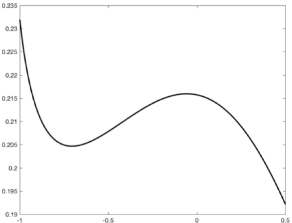
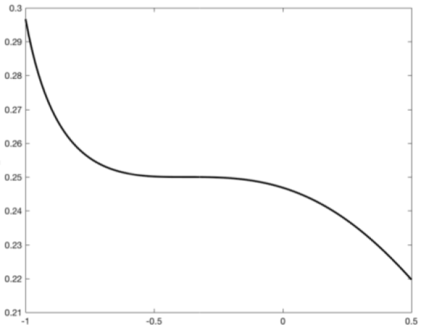
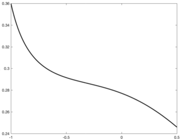
is a universal unfolding. The geometry of this universal unfolding is shown in Figure 1. Here, the singularity occurs when and it is a chair homeostasis point, Figure 1(b). When there is no singularity at but the plateau persists all near . The difference is that when the plateau has two nondegenerate singular points, Figure 1(a) and when the plateau has no singular points, Figure 1(c). See [26] for details.
Example 2.12 (Multiple Input Parameters).
We will consider the case. Table 1 summarizes the classification when , so . Here the list is restricted to codimension . The associated geometry, especially for universal unfoldings, is described in [22, 49, 112] up to codimension 4. Singularities of much higher codimension have also been classified, but the complexities increase considerably. For example, Arnold [12] provides an extensive classification up to codimension 10 (for the complex analog). Note that in the case the normal forms for appear again, but now there is an extra quadratic term . This term is a consequence of the splitting lemma in singularity theory, arising here when the Hessian of has rank 1 rather than rank 0 (corank 1 rather than corank [22, 112, 142]. The presence of the term affects the range over which changes when varies, but not when varies.
The standard geometric features considered in catastrophe theory focus on the gradient of the function in normal form. In contrast, what matters here is the function itself. Specifically, we are interested in the region in the -space where the function is approximately constant, i.e. the plateau of .
More specifically, for each normal form we choose a small and form the set
| (2.19) |
This is the -plateau region on which is approximately constant, where specifies how good the approximation is. Even though the definition of infinitesimal homeostasis is qualitative it is possible to extract quantitative bounds on the size of the plateau using Taylor’s theorem with remainder. See [56, Chap. 5] for details.
As we mentioned before, if is perturbed slightly (by variation of the suppressed parameters), the plateau varies continuously. Therefore, one can compute the approximate plateau by focusing on the singularity, rather than on its universal unfolding. In other words, for sufficiently small perturbations plateaus of singularities depend mainly on the singularity itself and not on its universal unfolding.
This observation is important because the universal unfolding has many zeros of the gradient of , hence ‘homeostasis points’ near which the value of varies more slowly than linear. However, this structure seems less important when considering the relationship of infinitesimal homeostasis with homeostasis. See the discussion of the unfolding of the chair summarized in [52, Figure 3].
The ‘qualitative’ geometry of the plateau – that is, its differential topology and associated invariants – is characteristic of the singularity. This offers one way to infer the probable type of singularity from numerical data; it also provides information about the region in which the system concerned is behaving homeostatically. We do not develop a formal list of invariants here, but we indicate a few possibilities.
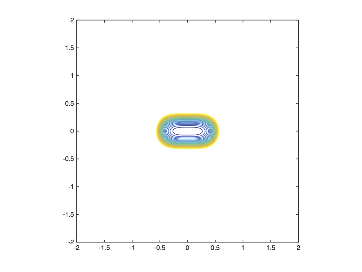
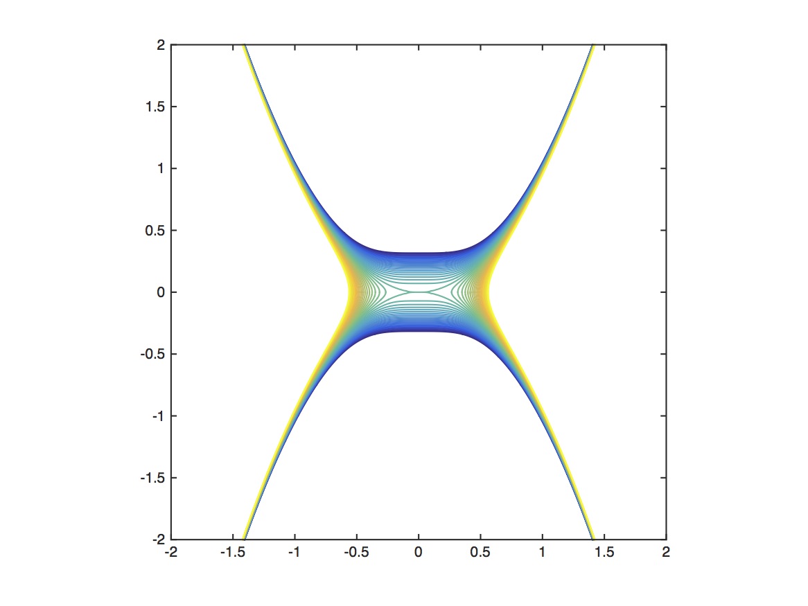
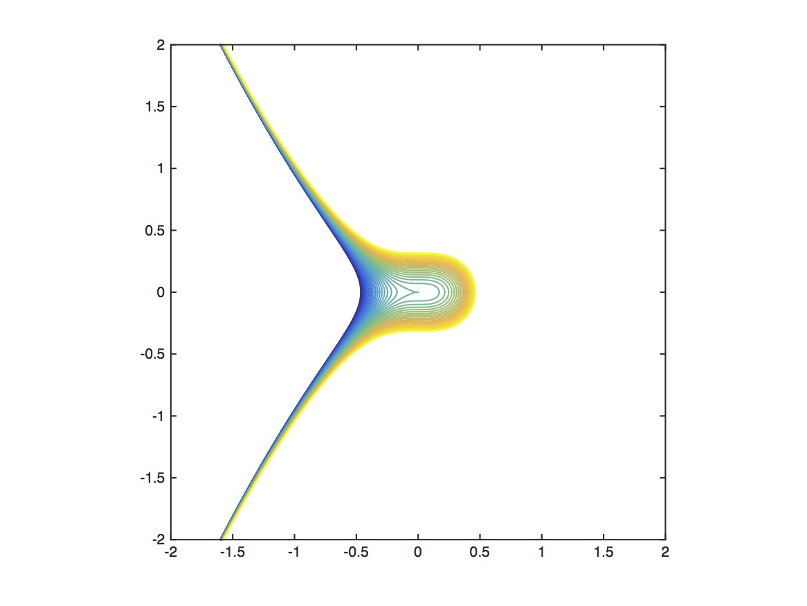
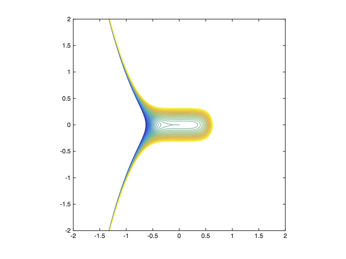
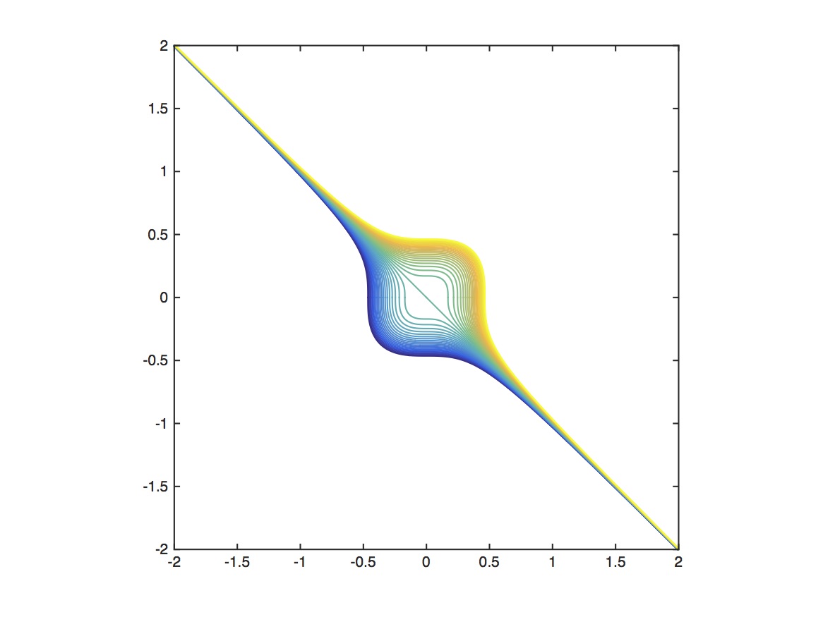
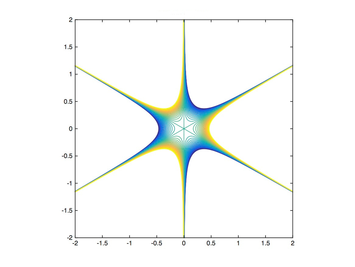
The main features of the plateaus associated with the six normal forms of Table 1 are illustrated in Figure 2. Figure plots, for each normal form, a sequence of contours from to ; the union is a picture of the plateaus. By unfolding theory, these features are preserved by small perturbations of the model, and by the choice of in (2.19) provided it is sufficiently small. Graphical plots of such perturbations (not shown) confirm this assertion.
| name | normal form | codim | universal unfolding |
| Morse (simple±) | 0 | ||
| fold (chair) | 1 | ||
| cusp± | 2 | ||
| swallowtail | 3 | ||
| hyperbolic umbilic | 3 | ||
| elliptic umbilic | 3 |
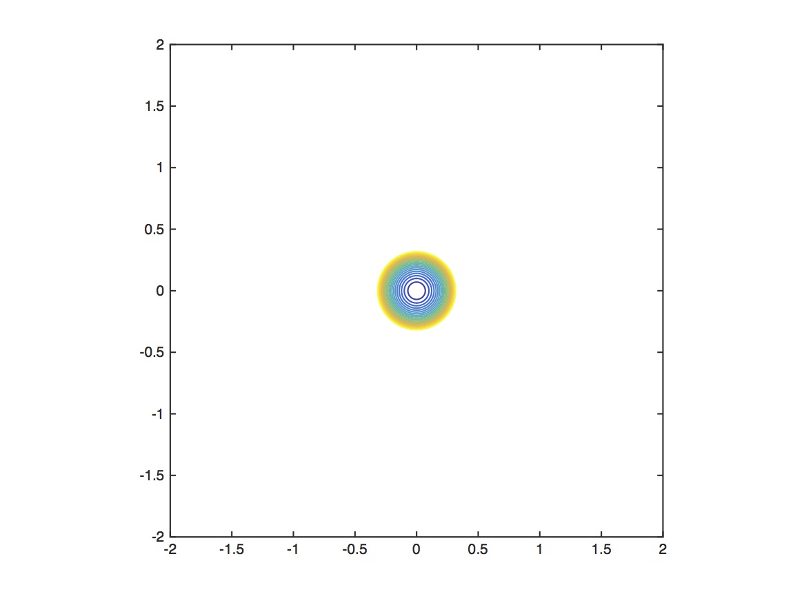
simple+ simple- cusp+ cusp-
chair swallowtail hyperbolic elliptic
The notion of infinitesimal homeostasis point can be generalized in several directions. For instance, Andrade et al. [3] consider the situation where the infinitesimal homeostasis point is at the boundary of the domain of the input-output function, which may be finite or infinity. They introduce the notion of asymptotic infinitesimal homeostasis for input-output functions defined on a domain of the form , for example. In this case we say that exhibits asymptotic infinitesimal homeostasis at if
In [3] the authors use some simple criteria for the existence of asymptotic infinitesimal homeostasis to study a model for copper homeostasis (see subsection 4.2).
Theorem 2.13.
Let , with be a smooth function.
-
[(1)]
-
1.
If exhibits near-perfect homeostasis on (i.e., it is upper and lower bounded on ) and is monotonic then exhibits asymptotic infinitesimal homeostasis.
- 2.
2.3 Homeostasis in Input-Output Networks
In this subsection we introduce input-output networks. This concept is crucial for the development of a rich combinatorial theory.
Definition 2.14.
An input-output network is a directed graph with a distinguished input node and a distinguished output node . The network is a core network if every node in is downstream from the input node and upstream from the output .
An admissible system of differential equations associated with has the form
| (2.20) | ||||
where is the input parameter, is the vector of state variables associated to nodes in , and is a smooth family of mappings on the state space . Note that appears only in the equation of system (2.20) corresponding to the input node.
We can write (2.20) as
We denote the partial derivative of the function associated to node with respect to the state variable associated to node , also called linearized couplings, by
We assume precisely when no arrow connects node to node . That is, is independent of when there is no arrow . This is a modeling assumption made in . Finally, we assume the genericity condition (2.11), which in this case reads
generically.
Suppose has a hyperbolic equilibrium at at . As before, we can define an input-output function defined on a neighborhood of .
Remark 2.15 (SISO Systems).
Each node in an input-output network corresponds to a one-dimensional state variable of the admissible system. In particular, the output node corresponds to a scalar quantity and the input parameter is a scalar quantity. The class of systems described by input-output networks can be seen as the class of single input, single output (SISO) systems. As we will see later, it is possible to extend this definition to include input-output networks with multiple input nodes, but a single input parameter and single output, and multiple inputs, single output (MISO).
Remark 2.16 (Input Node Output Node).
In Definition 2.14 we explicitly exclude the possibility that the output node is one of the input nodes. For now, this assumption is taken into account purely for the sake of convenience. In fact, all the results should be valid when the input output, but then all the theorems and proofs should be properly adapted to take this particular case into account. This possibility will be considered in greater detail in Subsection 4.2
Remark 2.17 (Multiple Outputs).
It is important to clarify why the input-output function should be always real-valued (-dimensional). This seems to be the correct way to formulate the notion of simultaneously tracking ‘multiple outputs’. Even in the control theoretic context of single input, multiple output (SIMO) and multiple input, multiple output (MIMO) the observable is real-valued (typically it is a linear functional). Actually, there is a singularity theoretic reason for this requirement, as well.
Let us try to define a two-output input-output function by considering a network with one input node and two output nodes and . Then the input-output function would be a mapping given by . This, in turn, would force us to consider more general coordinate changes on the target space (recall that in the real-valued situation the action of the right equivalence on the target is by a translation by a constant). Even in this simple two-output case one is led to consider general network preserving coordinate changes [53, 8]. Typically, the most natural coordinate change on that preserves the network structure is by a diagonal diffeomorphism , given by , where are diffeomorphisms. The set of smooth mappings of the form , with the equivalence relation generated by a pair of diffeomorphisms , where acts on the source and is a diagonal diffeomorphism acting on the target is called the set of divergent diagrams [95]. The classification of singularities of divergent diagrams have been obtained and the conclusion is that all ‘degenerate’ singularities have infinite codimension [36, 37, 38, 95]. Therefore, we would not be able to define an analogue of chair homeostasis (nor any other higher order singularity) in this setting.
Wang et al. [134] obtain a formula for the derivative of the input output function , with respect to , that is a particular case of formula (2.5) for input-output networks. Here, the observable is the projection onto the output coordinate. However, in this case the formula for is much simpler than the general case and provides a straightforward criterion for the occurrence of homeostasis in an input-output network.
The homeostasis matrix of (2.20) is the matrix is obtained from the Jacobian matrix of (2.20) by deleting its first row and last column. Indeed
where and are both functions of as in (2.20). More precisely:
Theorem 2.18 ([134, lemma 1.5]).
The derivative of the input-output function , with respect to is given by
| (2.21) |
Therefore, (2.20) undergoes infinitesimal homeostasis at if and only if , evaluated at .
Homeostasis in a given network can be determined by analyzing a simpler network that is obtained by eliminating certain nodes and arrows from . We call the network formed by the remaining nodes and arrows the core subnetwork.
Definition 2.19.
A node in a network is downstream from a node in if there exists a path in from to . Node is upstream from node if is downstream from .
These relationships are important when trying to classify infinitesimal homeostasis. For example, if the output node is not downstream from the input node , then the input-output function is identically constant in . Although technically this is a form of infinitesimal homeostasis, it is an uninteresting form.
Definition 2.20.
Let be an input-output network.
-
[(a)]
-
1.
The input-output network is a core network if every node is both upstream from the output node and downstream from the input node.
-
2.
Every input-output network has a core subnetwork whose nodes are the nodes in that are both upstream from the output node and downstream from the input node and whose arrows are the arrows in whose head and tail nodes are both nodes in .
Theorem 2.21 ([134, Thm. 2.4]).
Let be an input-output network and let be the associated core subnetwork. The input-output function associated with has a point of infinitesimal homeostasis at if and only if the input-output function associated with has a point of infinitesimal homeostasis at .
It follows from Corollary 2.21 that classifying infinitesimal homeostasis for networks is equivalent to classifying infinitesimal homeostasis for the core subnetwork .
Definition 2.22.
Let and be two input-output networks with the same number of nodes.
-
[(a)]
-
1.
We say that and are core equivalent if the determinants of their homeostasis matrices are identical as polynomials in the variables .
-
2.
A backward arrow is an arrow whose head is the input node or whose tail is the output node .
Corollary 2.23.
If two core networks differ from each other by the presence or absence of backward arrows, then the core networks are core equivalent.
Proof 2.24.
The linearized couplings associated to backward arrows are of the form and , which do not appear in the homeostasis matrix . ∎
Therefore, backward arrows can be ignored when computing infinitesimal homeostasis with the homeostasis matrix . However, backward arrows cannot be totally ignored, since they are involved in the determination of both the equilibria of (2.20) and their stability.
Corollary 2.23 can be generalized to a theorem giving necessary and sufficient graph theoretic conditions for core equivalence [134, Theorem 3.3].
Before proceeding to the classification results, we provide context for our results by looking at some of the biochemical models discussed by Reed in [115]. In doing so we show that input-output networks form a natural category in which homeostasis may be explored.
2.4 -node Input-Output Networks: Biochemical Networks
There are many examples of biochemical networks in the literature. In particular examples, modelers decide which substrates are important and how the various substrates interact. The network resulting from the detailed modeling of the production of extracellular dopamine (eDA) by Best et al. [18] and Nijhout et al. [103]. These authors derive a differential equation model for this biochemical network and use the results to study homeostasis of eDA with respect to variation of the enzyme tyrosine hydroxylase (TH) and the dopamine transporters (DAT).
In another direction, relatively small biochemical network models are often derived to help analyze a particular biochemical phenomenon. We present four examples; three are discussed in Reed et al. [115] and one in Ma et al. [89]. These examples belong to a class that we call biochemical input-output networks and will help to interpret the mathematical results.
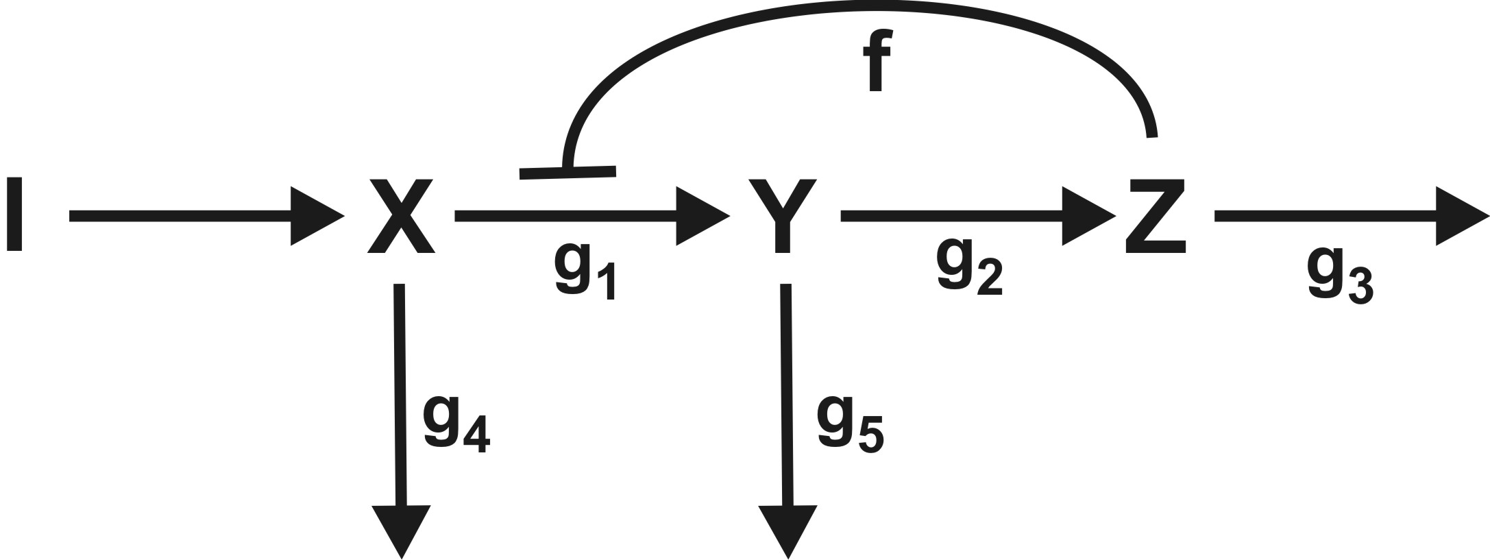
Example 2.25 (Feedforward Excitation).
The input-output network corresponding to feedforward excitation is in Figure 3. This motif occurs in a biochemical network when a substrate activates the enzyme that removes a product. The standard biochemical network diagram for this process is shown in Figure 3(a). Here , , are the names of chemical substrates and their concentrations are denoted by lower case , , . Each straight arrow represents a flux coming into or going away from a substrate. The differential equations for each substrate simply state that the rate of change of the concentration is the sum of the arrows going towards the substrate minus the arrows going away (conservation of mass). The curved line indicates that substrate is activating an enzyme.

Both diagrams in Figure 3 represent the same information, but in different ways. Figure 3(b) uses nodes to represent variables, and arrows to represent couplings. In other areas, conventions can differ, so it is necessary to translate between the two representations. The simplest method is to write down the model ODEs.
The equations corresponding to the biochemical network in Figure 3 (a) are as follows
| (2.22) |
In this motif, one path consists of two excitatory couplings: from to and from to . The other path is an excitatory coupling from to the synthesis or degradation of and hence is an inhibitory path from to having a negative sign.
It is shown in [115] (and reproduced using the abstract theory in [58]) that the model equations (2.22) for feedforward excitation leads to infinitesimal homeostasis at if
| (2.23) |
where is a stable equilibrium.
Figure 3(b) redraws the diagram in Figure 3(a) using the abstract definition of input-output network, together with some extra features (the signs along the arrows) that are crucial to this particular application. We consider to be a distinguished input variable, with as a distinguished output variable, while is an intermediate regulatory variable. Accordingly we change notation and write , and .
The general form of the equations associated to the diagram of Figure 3(b) in the state variables is
| (2.24) |
In Figure 3(b) these variables are associated with three nodes . Each node has its own symbol: a square for , circle for , and triangle for . Here these symbols are convenient ways to show which type of variable (input, regulatory, output) the node corresponds to. Arrows indicate that the variables corresponding to the tail node occur in the component of the ODE corresponding to the head node. For example, the component for is a function of , , and . We therefore draw an arrow from to and an arrow from to . We do not draw an arrow from to itself, however: by convention, every node variable can appear in the component for that node. In a sense, the node symbol (circle) represents this ‘internal’ arrow.
The Jacobian of (2.24) is
The bottom-left block of is the homeostasis matrix of of (2.24). Since is lower triangular, it follows that linear stability occurs when the linearized self-couplings are all negative.
The mathematics described here shows that infinitesimal homeostasis occurs in the system in the second column of (2.22) if and only if
| (2.25) |
at the stable equilibrium . It is easy to see that (2.23) is a particular case of (2.25).
Figure 3(b) incorporates some additional information. The arrow from to node indicates that occurs in the equation for as the input parameter. Similarly the arrow from node to the symbol indicates that node is the output node. Finally, the signs indicate which arrows are excitatory or inhibitory. This extra information is special to biochemical networks and does not appear as such in the general theory.
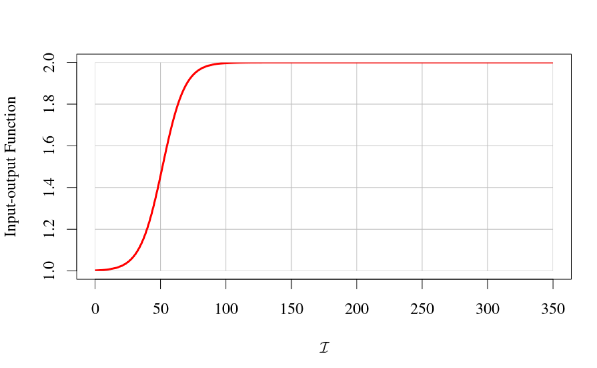
In Figure 7(a) we show the graph of the input-output function , as a function of the input parameter , for the model equations (2.22). Here, , and
where and the infinitesimal homeostasis point occurs at . In this case, it can be shown that the infinitesimal homeostasis occurring at and is in fact a chair singularity and is the unfolding parameter, see [115] for details.
Example 2.26 (Product inhibition).
Also called feedback inhibition, this is probably one of the simplest and best known homeostatic mechanisms in biochemistry. In its simplest form, feedback inhibition means that the product of a biochemical chain inhibits one or more of the enzymes involved in its own synthesis. Thus if the concentration of the end product goes up, synthesis is slowed, and if the concentration goes down, the inhibition is partially withdrawn and the synthesis goes faster. More specifically, suppose that substrate influences , which influences , and inhibits the flux from to . The biochemical network for this process is shown in Figure 4(a).

This time the model equations for Figure 4(a) are
| (2.26) |
and the input-output equations associated to (2.26) can be read directly from Figure 4(b)
| (2.27) |
Reed et al. [115] explain that, due to biochemical reasons, the model equation 2.26 for product inhibition must satisfy some additional constraints
| (2.28) |
Our general mathematical results show that the model system (2.26) exhibits infinitesimal homeostasis at a stable equilibrium if and only if
| (2.29) |
That is, either
| (2.30) |
It follows from (2.28) and (2.30) that the model equation (2.26) cannot exhibit infinitesimal homeostasis. Nevertheless, Reed et al. [115] show that this biochemical network equations do exhibit near-prefect homeostasis; that is, the output is almost constant for a broad range of input values . In the general admissible equations 2.27 infinitesimal homeostasis can occur generically. However, due to the special form of the model equation (2.26) and the additional constraints (2.28), infinitesimal homeostasis is forced to occur at the ‘boundary of the universal unfolding’, where or .
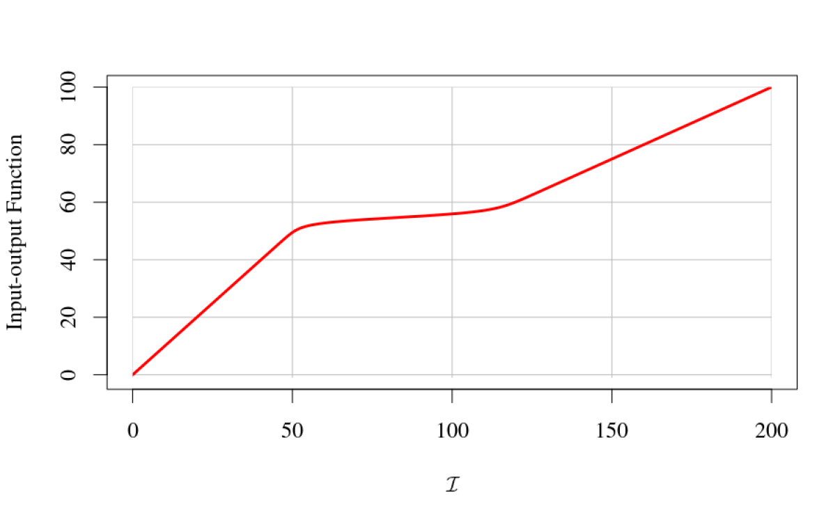
In Figure 7(b) we show the graph of the input-output function , as a function of the input parameter , for the model equations (2.26). Here, and
where and . As explained above infinitesimal homeostasis cannot occur in this model equation. The almost flat region occurs from to , see [115] for details.
Example 2.27 (Substrate Inhibition).
The biochemical network model for substrate inhibition is given in Figure 5(a), and the associated model system is given in the first column of (2.31). This biochemical network and the model system are discussed in Reed et al. [115].
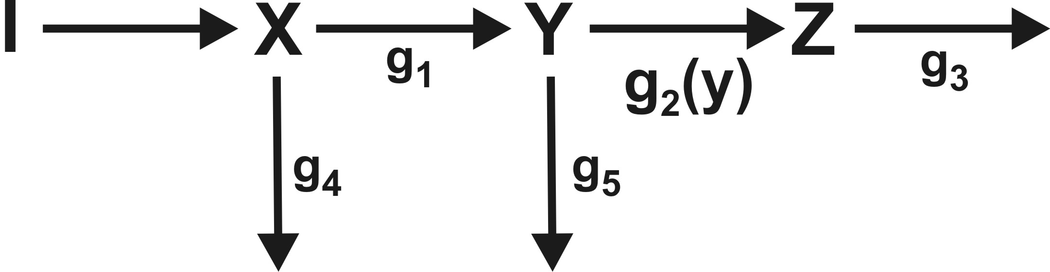

The equations associated to the diagram for substrate inhibition from Figure 5(a) are
| (2.31) |
Reed et al. [115] provides a biochemical justification for taking for , whereas the coupling (or kinetics term) can change sign.
That model system of ODEs can be easily translated to the input-output system
| (2.32) |
The Jacobian of (2.32) is
The bottom-left block of is the homeostasis matrix of of (2.32). Since is lower triangular, it follows that linear stability occurs when the linearized self-couplings are all negative.
The mathematics described here shows that the condition for infinitesimal homeostasis is
| (2.33) |
Note that this is the same condition as in the case of product inhibition (2.29). Therefore, the network for product inhibition and the network for substrate inhibition are core equivalent. In fact, the network for substrate inhibition form Figure 5 can be obtained from the network from for product inhibition form Figure 4 by removing two backward arrows: and . These two backward arrows correspond to two off-diagonal entries in the last column of the Jacobian matrix that are absent in the substrate inhibition. As explained before, they do not affect the homeostasis matrix but can influence the linear stability of the system. In fact, as noted above, the absence of these two arrows in the substrate inhibition network renders the Jacobian Matrix lower triangular and so the linear stability depends only on the linearized self-couplings of the three nodes.
On the assumption that , infinitesimal homeostasis is possible only if the coupling is neutral, that is, if at the equilibrium point. This conclusion agrees with the observation in [115] that can exhibit infinitesimal homeostasis in the substrate inhibition motif if the infinitesimal homeostasis is built into the kinetics for the function which controls the coupling between and .
Reed et al. [115] note that neutral coupling can arise from substrate inhibition of enzymes, enzymes that are inhibited by their own substrates. See the discussion in [116]. This inhibition leads to reaction velocity curves that rise to a maximum (the coupling is excitatory) and then descend (the coupling is inhibitory) as the substrate concentration increases. Infinitesimal homeostasis with neutral couplings arising from substrate inhibition often has important biological functions and has been estimated to occur in about of enzymes [116]. In the 1930s, Haldane [63] introduced the concept of substrate inhibition in which the substrate of the reaction itself inhibits the enzyme that catalyzes the reaction. Golubitsky and Wang [58] have called homeostasis similar to the one occurring in substrate inhibition Haldane homeostasis, since it arise from neutral coupling, that is, the linearized coupling between to nodes changes sign as the input parameter is varied.
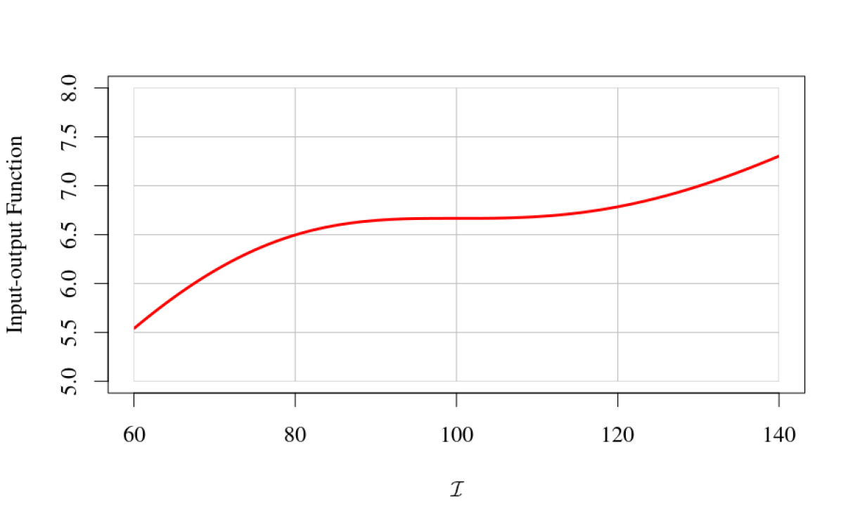
In Figure 7(c) we show the graph of the input-output function , as a function of the input parameter , for the model equations (2.31). Here, and
where . Here, unlike in the case of product inhibition, infinitesimal homeostasis can occur by a Haldane type mechanism. After an initial growth from to over the -range the curve becomes flat and the system exhibits perfect homeostasis for .
Example 2.28 (Negative Feedback Loop).
Here, each enzyme , , in the feedback loop motif, see Figure 6(a) can have active and inactive forms. In the kinetic equations (2.34) the coupling from to is non-neutral according to Ma et al. [89]. Hence, in this model only null-degradation homeostasis is possible. In the kinetic equations in the model the equation does not depend on and homeostasis can only be perfect homeostasis. However, this model is a simplification based on saturation in [89]. In the original system does depend on and we expect standard null-degradation homeostasis to be possible in that system. The corresponding input-output network to the negative feedback loop motif in Figure 6(a) is shown in Figure 6(b).


The equations associated to the negative feedback loop diagram of Figure 6(a) are
| (2.34) |
where , , , , , , , , , , , are 12 constants. That model system of ODEs is easily translated to the input-output system
| (2.35) |
The mathematics described here shows that the model system (2.35) exhibits infinitesimal homeostasis if and only
| (2.37) |
That is, either
| (2.38) |
The first case is the Haldane homeostasis type discussed before. The second case is called null-degradation, since it arises when the degradation constant (i.e., the linearized self-coupling) of the regulatory node changes sign when the input parameter is varied.
Stability of the equilibrium in this motif implies negative feedback between and . From the Jacobian matrix 2.36 of (2.35) it follows that, at null-degradation homeostasis (), linear stability implies that
| (2.39) |
Conditions (2.39) imply that both the input node and the output node need to degrade and the couplings and must have opposite signs. This observation agrees with [89] that homeostasis is possible in the network motif Figure 6(a) if there is a negative loop between and and when the linearized internal dynamics of is zero. Therefore, the negative feedback is ‘forced’ by the condition for null-degradation and stability.
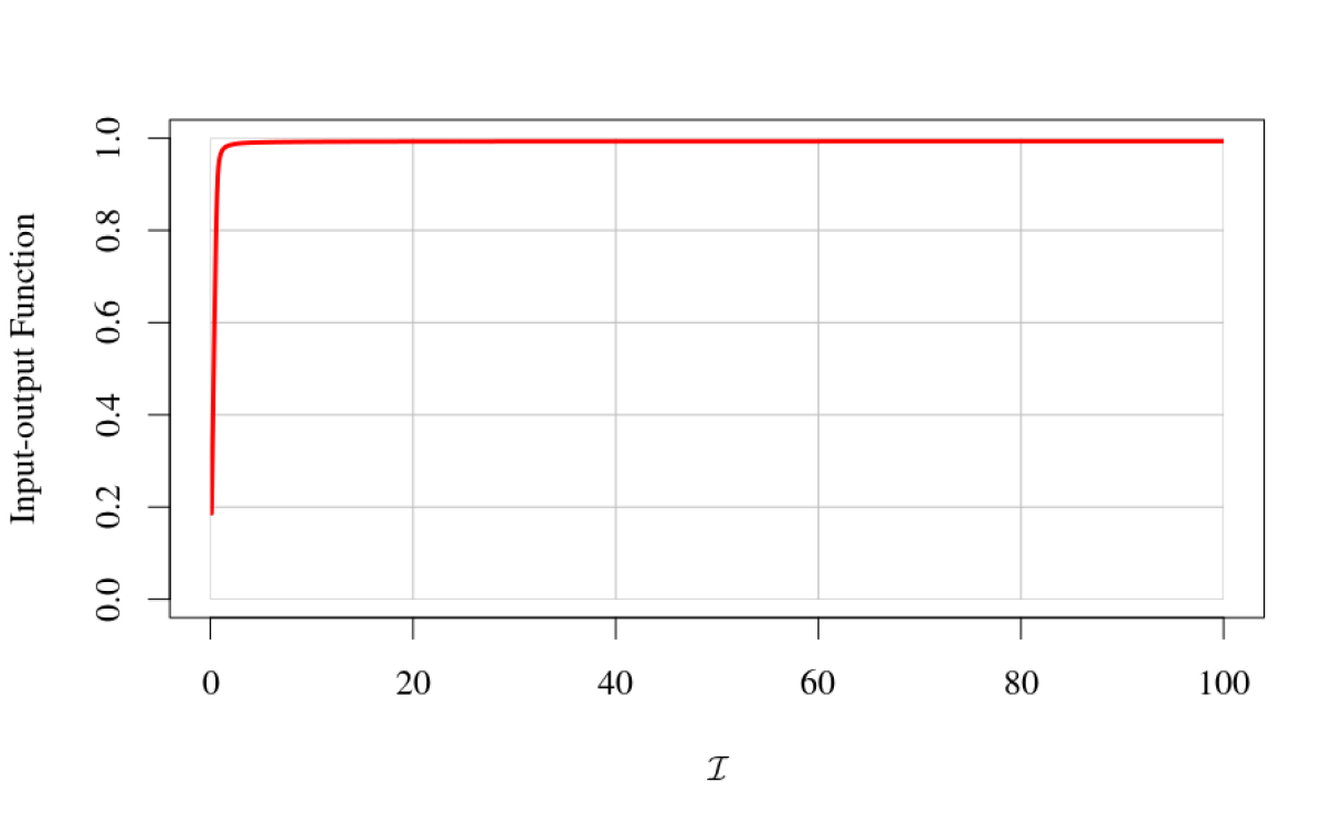
In Ferrell [46] the author reviews some motifs that are capable of displaying perfect or near-perfect homeostasis and presents a simplification of biochemical example of Ma et al. [89], that exhibits null-degradation homeostasis. In Figure 7(d) we show the graph of the input-output function , as a function of the input parameter , for the model equations of [46, Fig 2]. After an almost instantaneous jump from to the curve becomes flat and the system exhibits, in fact perfect homeostasis for .
As we have seen in these four examples of -node biochemical networks there are plenty of possibilities of homeostatic behaviors already in very small networks. Golubitsky and Wang [58] started a systematic investigation of the -node input-output networks in an attempt to organize the understanding of the biochemical examples. Their success was the motivation for Wang et al. [134] to undertake the general case of an -node input-output network and eventually led to a general theory. In hindsight, their theorem for classification of the -node input-output networks can be simply stated as
Theorem 2.29 ([58, 134]).
There are core equivalence classes of -node input-output core networks with input node output node. Representatives are given by: (i) the Feedforward Excitation motif, (ii) the Substrate Inhibition motif and (iii) the Negative Feedback motif. Any other -node input-output network with two distinguished nodes can be obtained from these representatives by adding or removing backward arrows.
As we shall see later, if we allow input node output node then there are two more core equivalence classes, thus giving a complete classification of all -node input-output networks (see subsection 4.2).
2.5 Homeostasis Patterns in Input-Output Networks
Now we consider the notion of a homeostasis pattern on a given input-output network . A homeostasis pattern is the set of nodes in (including the output node ) such that the node coordinate , as a function of , satisfies . In other words, a homeostasis pattern is a set of nodes of , that includes the output node , and all nodes in are simultaneously (infinitesimally) homeostatic at a given parameter value .
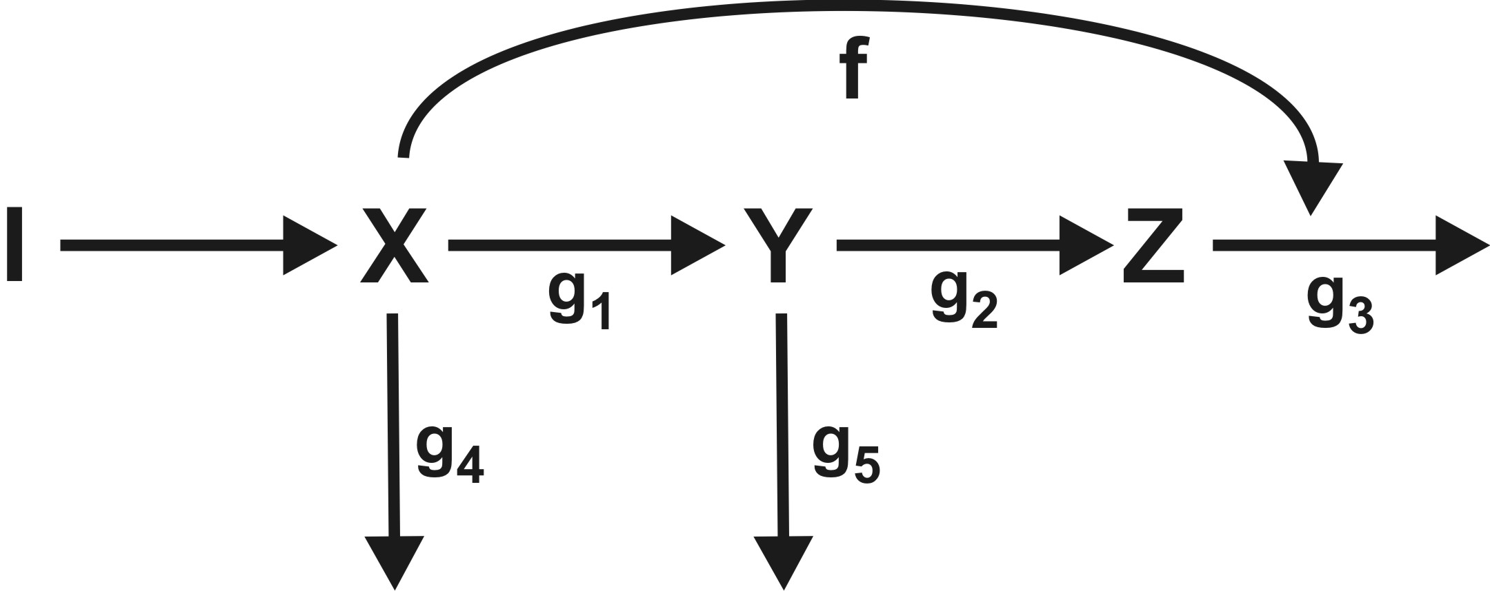
However, before going into the details of this theory, we use such calculations to give some indication of why the input-output network in Figure 8 has exactly the homeostasis patterns exhibited in Figure 9.
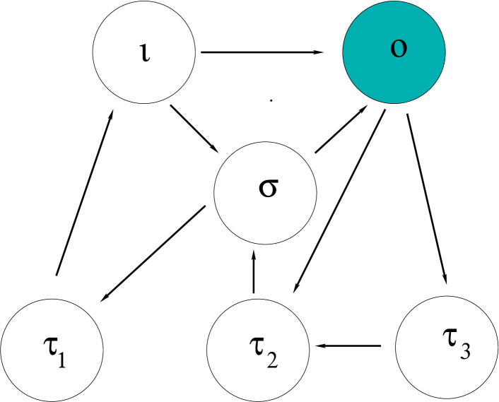
Consider for example the node input-output network shown in Figure 8.

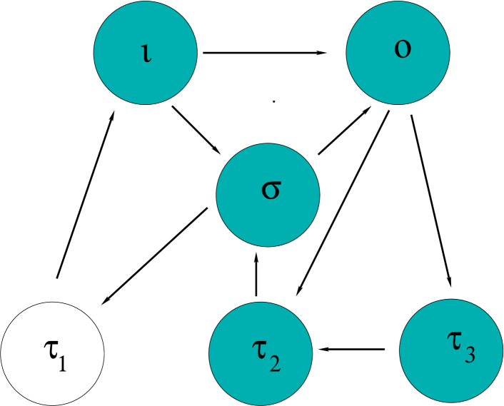
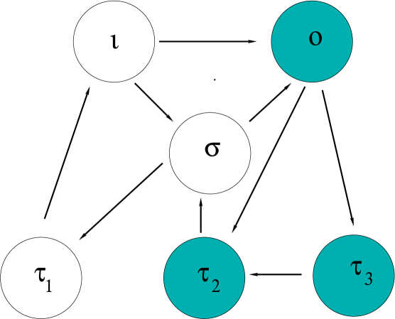
Although there are exactly subsets of nodes of including the output node , only subsets define homeostasis patterns: , , and . These homeostasis patterns can be graphically represented by coloring the nodes of that are homeostatic (see Figure 9).
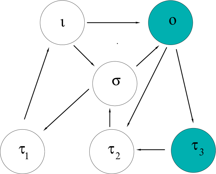
The admissible system of parametrized equations for the network in Figure 8, in coordinates , is:
| (2.40) |
The homeostasis matrix is obtained from the Jacobian matrix of (2.40) and is given by
Using row and column expansion it is straightforward to calculate
| (2.41) |
Theorem 2.18says that the input-output function undergoes infinitesimal homeostasis at if and only if , evaluated at . Here is the equilibrium used to construct the input-output function. The expression is a multivariate polynomial in the partial derivatives of the components of the admissible vector field. As a polynomial, is reducible with irreducible factors, so if and only if one of its irreducible factors vanishes.
According to [134] these irreducible factors determine the homeostasis types (see section 3). Hence, (2.40) has homeostasis types. One of the main results of this paper says that each homeostasis type determines a unique homeostasis pattern. Moreover, our theory gives a purely combinatorial procedure to find the set of nodes that belong to each homeostasis pattern. When applied to Figure 8 it yields the four patterns in Figure 9.
In a simple example such as Figure 8 it is also possible to find the sets of nodes in each homeostasis pattern by a ‘bare hands’ calculation based on the admissible ODEs. Here this calculation serves as a check on the results. Direct calculations with the ODEs can, of course, be used instead of the combinatorial approach in sufficiently simple cases.
Finally, we determine the four homeostasis patterns by direct calculation. We do this by assuming that there is a one-parameter family of stable equilibria where using implicit differentiation with respect to (indicated by ′), and expanding (2.40) to first order at . The linearized system of equations is
| (2.42) |
Next we compute the homeostasis patterns corresponding to the homeostasis types of (2.40).
(a) Homesotasis Type: ;
Homeostatic nodes:
Equation (2.42) becomes
| (2.43) |
Since and are generically nonzero at homeostasis, the fourth equation implies that generically and are nonzero. The second and sixth equations can be rewritten as
Generically the right hand side of this matrix equation at is nonzero; hence generically and are also nonzero. The third equation implies that generically is nonzero. Therefore, in this case, the only homeostatic node is .
(b) Homeostasis Type: ;
Homeostatic nodes:
In this case (2.42) becomes
| (2.44) |
The fifth equation implies that generically . The fourth equation implies that generically . The third equation implies that generically and the sixth equation implies that generically is zero. It follows that the infinitesimal homeostasis pattern is .
(c) Homeostasis Type: ;
Homeostatic nodes:
Equation (2.42) becomes
| (2.45) |
The fourth or fifth equation implies that . The first and sixth equations imply that , , and are nonzero. The third equation implies that generically is nonzero. Hence the infinitesimal homeostasis pattern is .
(d) Homeostasis Type: ; Homeostatic nodes
To repeat, Equation (2.42) is
| (2.46) |
The fifth equation implies generically that and the fourth equation implies generically that . Again, the second and sixth equations can be rewritten in matrix form as
Hence generically and are nonzero. The third equation implies that is nonzero. Hence the homeostatic nodes are .
The homeostasis types of (2.40) with the corresponding homeostasis patterns are summarized in Table 2.
| Homeostasis Type | Homeostasis Pattern | Figure 9 |
| (a) | ||
| (b) | ||
| (c) | ||
| (d) |
In principle the homeostasis patterns can be computed in the manner shown above; but in practice this becomes very complicated.
3 Classification
In this section we describe the theory of Wang et al. [134] and Duncan et al. [40] about the classification of homeostasis types and homeostasis patterns in an input-output network, respectively.
3.1 Homeostasis Subnetworks
In [134] the authors show that the determination of infinitesimal homeostasis in an input-output networks reduces to the study of core networks. We assume throughout that the input-output networks are core networks.
The first main result of [134] is the observation that one can apply the Frobenius-König [118, 23] theorem to the homeostasis matrix and obtain a decomposition of into its irreducible factors.
Theorem 3.1 ([134, Theorem 1.11]).
Assume (2.20) has a hyperbolic equilibrium at . Then there are permutation matrices and such that is block upper triangular with square diagonal blocks . The blocks are irreducible in the sense that each cannot be further block triangularized. It follows that
| (3.47) |
is an irreducible factorization of .
Definition 3.2.
Let be an input-output network and its homeostasis matrix. Each irreducible square block in (3.47) is called a homeostasis block. Further, we say that infinitesimal homeostasis in is of homeostasis type if for all , and .
Remark 3.3.
Let be a homeostasis type and let
A chair point of type occurs at if and .
In principle every homeostasis type can lead to infinitesimal homeostasis, that is, for some input value . For simplicity, we say that node is homeostatic at .
Let be a diagonal block of , hence has degree . Since the entries of are entries of , these entries have the form ; that is, the entries are either (if is not an arrow in ), self-coupling (if ), or coupling (if is an arrow in ).
Since and in Theorem 3.1 are constant permutation matrices, all entries in each row (resp. column) of must lie in a single row (resp. column) of . Hence, has the form
| (3.48) |
It follows that the number of self-coupling entries of are the same no matter which permutation matrices and are used to bring to the block-diagonal form.
Theorem 3.4 ([134, Theorem 4.4]).
Each submatrix has either or self-coupling entries.
Definition 3.5.
The homeostasis class of an irreducible component of degree is appendage if has self-couplings and structural if has self-couplings.
Now we can associate a homeostasis subnetwork with each homeostasis block and give a graph-theoretic description of each .
Definition 3.6.
The homeostasis subnetwork of associated with the homeostasis block is defined as follows. The nodes in are the union of nodes and where is a nonzero entry in and the arrows of are the union of arrows where .
In order to give a combinatorial characterization of the structural and appendage homeostasis subnetworks we need some simple concepts from graph theory.
Definition 3.7.
Let be a core input-output network.
-
[(a)]
-
1.
A simple path from node to node in is a directed path that starts at , ends at , and visits each node on the path exactly once. We denote the existence of a simple path from to by . A simple cycle is a simple path whose first and last nodes are identical.
-
2.
An -simple path is a simple path from the input node to the output node .
-
3.
A node is simple if it lies on an -simple path. A node is appendage if it is not simple.
-
4.
A simple node is super-simple if it lies on every -simple path.
We typically use to denote a simple node, to denote a super-simple node, and to denote an appendage node when the type of the node is assumed a priori. Otherwise, we use to denote an arbitrary node. Note that and are super-simple nodes.
Let be the super-simple nodes, where and . The super-simple nodes are totally ordered by the order of their appearance on any -simple path, and this ordering is independent of the -simple path. We denote an -simple path by
where indicates a simple path from to . The ordering of the super-simple nodes is denoted by
and is a total ordering. The ordering extends to a partial ordering of simple nodes, as follows. If there exists a super-simple node and an -simple path such that
then the partial orderings
are valid. In this partial ordering every simple node is comparable to every super-simple node but two simple nodes that lie between the same adjacent super-simple nodes need not be comparable.
We recall the definition of transitive (or strong) components of a network. Two nodes are equivalent if there is a path from one to the other and back. A transitive component is an equivalence class for this equivalence relation.
Definition 3.8.
-
[(a)]
-
1.
Let be an -simple path. The complementary subnetwork of is the network whose nodes are nodes that are not in and whose arrows are those that connect nodes in .
-
2.
An appendage node is super-appendage if for each containing , the transitive component of in consists only of appendage nodes.
Note that this definition of super-appendage leads to a slightly different, but equivalent, definition of homeostasis subnetwork to the one given in [134]. However, this change enables us to define pattern networks in a more straightforward way (see Remark 3.11).
Now we start with the definition of structural subnetworks.
Definition 3.9.
Let and be two consecutive super-simple nodes. Then the simple subnetwork , the augmented simple subnetwork , and the structural subnetwork are defined in four steps as follows.
-
[(a)]
-
1.
The simple subnetwork consists of simple nodes where
and all arrows connecting these nodes. Note that does not contain the super-simple nodes and , and can be the empty set.
-
2.
An appendage but not super-appendage node is linked to if for some complementary subnetwork the transitive component of in is the union of , nodes in , and non-super-appendage nodes. The set of -linked appendage nodes is the set of non-super-appendage nodes that are linked to .
-
3.
The augmented simple subnetwork is
and all arrows connecting these nodes.
-
4.
The structural subnetwork consists of the augmented simple subnetwork and adjacent super-simple nodes. That is
and all arrows connecting these nodes.
Note that an structural subnetwork is itself an input-output network, with input node and output node .
Next we define the appendage subnetworks, which were defined in Section 1.7.2 of [134] as any transitive component of the subnetwork consisting only of appendage nodes and the arrows between them.
Definition 3.10.
An appendage subnetwork , is a transitive component of the subnetwork of super-appendage nodes.
Remark 3.11.
In [134] the authors define an appendage subnetwork as a transitive component of appendage nodes that satisfy the no cycle condition. The no-cycle condition is formulated in terms of the non-existence of a cycle between appendage nodes in and the simple nodes in for all simple -simple paths . Here, we define an appendage subnetwork as a transitive component of super-appendage nodes, which are defined in terms of transitive components with respect to for all simple -simple paths . These two definitions are equivalent because two nodes belong to the same transitive component if and only if both nodes lie on a (simple) cycle.
Theorem 3.12 ([134]).
Let be a homeostasis subnetwork of with corresponding diagonal block .
-
[(1)]
-
1.
If is structural then for some . Moreover, is an input-output network, hence is an homeostasis matrix and
where is the homeostasis matrix of .
-
2.
If is appendage then for some . Moreover, is a network without any distinguished node, hence is a jacobian matrix and
where is the jacobian matrix of .
Theorem 3.12 says that the network decomposes into subnetworks , each of which is of two types: structural or appendage. Two of these subnetworks may have common nodes only when they are consecutive structural subnetworks. Furthermore, the irreducible factors of can be obtained directly from the set of homeostasis subnetworks.
3.2 Homeostasis Patterns
Definition 3.13.
A homeostasis pattern corresponding to the homeostasis block at is the collection of all nodes, including the output node , that are simultaneously forced to be homeostatic at .
Definition 3.14.
Assume that the output node is homeostatic at , that is, for the input value .
-
[(a)]
-
1.
We call the homeostasis subnetwork homeostasis inducing if at .
-
2.
Homeostasis of a node is induced by a homeostasis subnetwork , denoted , if is generically homeostatic whenever is homeostasis inducing.
-
3.
A homeostasis subnetwork induces a subset of nodes (), if for each node .
By definition, every homeostasis subnetwork induces homeostasis in the output node , that is, .
In this subsection we construct the homeostasis pattern network associated with (see Definition 3.21), which serves to organize the homeostasis subnetworks and to clarify how each homeostasis subnetwork connects to the others.
The homeostasis pattern network is defined in the following steps. First, we define the structural pattern network in terms of the structural subnetworks of . Second, we define the appendage pattern network in terms of the appendage subnetworks of . Finally, we define how the nodes in connect to nodes in and conversely.
Definition 3.15.
The structural pattern network is the feedforward network whose nodes are the super-simple nodes and the backbone nodes , where is the augmented structural subnetwork treated as a single node. The nodes and arrows of are given as follows.
| (3.49) |
If a structural subnetwork consists of an arrow between two adjacent super-simple nodes (Haldane type) then the corresponding augmented structural subnetwork is the empty network; nevertheless the corresponding backbone node must be included in the structural pattern network .
Definition 3.16.
The appendage pattern network is the network whose nodes are the components in the condensation of the subnetwork of super-appendage nodes. Such a node is called an appendage component. An arrow connects nodes and if and only if there are super-appendage nodes and such that in .
Definition 3.17.
Let be a directed graph. Consider the equivalence relation given by path equivalence on the set of nodes of . The equivalence classes are the path components of . Let be the quotient graph called the condensation of . That is, the nodes of are the path components of and the arrows of are defined as follows. There is a directed arrow form path component to path component if there are nodes , and a direct arrow form to .
To complete the homeostasis pattern network, we describe how the nodes in and the nodes in are connected. To do so, we take advantage of the feedforward ordering of the nodes in and the feedback ordering of the nodes in .
Definition 3.18.
A simple path from to is an appendage path if some node on this path is an appendage node and every node on this path, except perhaps for and , is an appendage node.
Definition 3.19 (How connects to ).
Given a node , we construct a unique arrow from to the structural pattern network in two steps:
-
[(a)]
-
1.
Consider the collection of nodes in for which there exists a simple node and appendage node , such that there is an appendage path from to .
-
2.
Let be a maximal node in this collection, that is, the most downstream in . It follows from (3.49) that is either a super-simple node or a backbone node . Maximality implies that is uniquely defined. We then say that there is an arrow from to .
Definition 3.20 (How is connected from ).
Given a node we choose uniquely an arrow from the structural pattern network to in two steps:
-
[(a)]
-
1.
Consider the collection of nodes in for which there exists a simple node and appendage node , such that there is an appendage path from to .
-
2.
Let be a minimal node in this collection, that is, the most upstream node in . Then is either a super-simple node or a backbone node , and the minimality implies uniqueness of . We then say that there is an arrow from to .
Since we consider only core input-output networks, all appendage nodes are downstream from and upstream from . Hence, for any node , there always exist nodes as mentioned above.
Definition 3.21.
The homeostasis pattern network is the network whose nodes are the union of the nodes of the structural pattern network and the appendage pattern network . The arrows of are the arrows of , the arrows of , and the arrows between and as described above.
Remark 3.22.
The super-simple nodes in correspond to the super-simple nodes of . Each super-simple node (for ) belongs to exactly two structural subnetworks and . Thus they are not associated to a single homeostasis subnetwork of .
It follows from Remark 3.22 that there is a correspondence between the homeostasis subnetworks of and the non-super-simple nodes of .
Remark 3.23.
-
[(a)]
-
1.
Each structural subnetwork corresponds to the backbone node . Note that the augmented structural subnetworks are not homeostasis subnetworks.
-
2.
Each appendage subnetworks corresponds to a appendage component .
-
3.
For simplicity in notation we let denote a node in . Further we let denote a non-super-simple node of and denote its corresponding homeostasis subnetwork.
The main point of introducing the homeostasis pattern network is to relate homeostatic induction between the set of homeostasis subnetworks of to induction between nodes in . In Definition 3.24 bellow we formalize this notion. Hence, every node in a homeostasis pattern (which can be backbone or appendage) is induced by either a backbone node or an appendage node in the homeostasis pattern network .
Definition 3.24.
Let be non-super-simple nodes and be a super-simple node. Let be the corresponding homeostasis subnetworks to . We say that induces , denoted by , if and only if . We say that induces , denoted by , if and only if .
We exclude super-simple nodes of from being ‘homeostasis inducing’ because they are not associated to a homeostasis subnetwork of (see Remark 3.22). However, when a backbone node induces homeostasis on other nodes of , it is the corresponding structural subnetwork , with its two super-simple nodes that induce homeostasis.
As explained before, the homeostasis pattern network allows us to characterize homeostasis patterns by reducing to four possibilities that are covered by Theorems 3.25 - 3.28.
Structural homeostasis patterns are given by the following two theorems.
Theorem 3.25 (Structural Structural).
A backbone node induces every node of the structural pattern network strictly downstream from , but no other nodes of .

Theorem 3.26 (Structural Appendage).
A backbone node induces every appendage component of whose (see Definition 3.20) is strictly downstream, but no other nodes of .
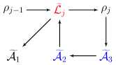
The appendage homeostasis patterns are characterized by the following two theorems.
Theorem 3.27 (Appendage Structural).
An appendage component induces every super-simple node of downstream from (see Definition 3.19), but no other super-simple nodes. Further, an appendage component induces a backbone node if and only if is strictly downstream from .
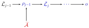
Theorem 3.28 (Appendage Appendage).
An appendage component induces an appendage component if and only if is strictly upstream from and every path from to in contains a super-simple node satisfying .
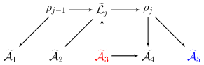
Example 3.29.
We consider homeostasis patterns for the admissible systems in (2.40) obtained from Figure 8. Specifically, we show how the theorems in this section lead to the determination of the homeostasis patterns that were derived by direct calculation from the equations (2.42). The corresponding homeostasis pattern network is shown in Figure 14. The answer is listed in Table 2.
Case (a) : homeostasis is induced by the node of . Theorem 3.27 shows induces , which is the only super-simple node of downstream from . And induces no backbone node. Theorem 3.28 shows induces no appendage component. Therefore, in this case the homeostasis pattern is .
Case (b) : homeostasis is induced by the node of . Theorem 3.27 shows induces , which are the super-simple nodes of downstream from . Also induces , which is the backbone node of downstream from . Theorem 3.28 shows induces , which are the nodes of downstream from and each path contains the super-simple node with or . Therefore, in this case the homeostasis pattern is .
Case (c) : homeostasis is induced by the node of . Theorem 3.27 shows induces , which is the super-simple nodes of downstream from . And induces no backbone node. Theorem 3.28 shows induces , which is the node of downstream from and each path contains the super-simple node with . Therefore, in this case the homeostasis pattern is .

Finally, we give three general results about the induction relation. First, in Theorem 3.30 we state that the induction relation is characterized by its behavior on homeostasis subnetworks. Next, in Theorems 3.31 we state that induction applies in at least one direction for distinct homeostasis subnetworks and that no subnetwork induces itself. Finally, in Theorem 3.32 we state that distinct subnetworks have distinct homeostasis patterns. That is, the set of nodes induced by a homeostasis subnetwork is unique among all homeostasis subnetworks. For proofs see [40].
Theorem 3.30.
Suppose and are distinct homeostasis subnetworks of . Let be a node of where . If , then .
Theorem 3.31.
Let be a homeostasis subnetwork of . Then generically . Moreover, let be some other homeostasis subnetwork of . Then one of the following relations holds:
-
[(a)]
-
1.
and ,
-
2.
and ,
-
3.
and .
Theorems 3.30 and 3.31 imply that each homeostasis subnetwork has a unique homeostasis pattern associated to it. Specifically:
Theorem 3.32.
Let and be two distinct homeostasis subnetworks of . Then the set of subnetworks induced by and the set of subnetworks induced by are distinct.
Theorem 3.32 implies that there is a bijective correspondence between homeostasis subnetworks of and homeostasis patterns supported by . Recall that theorem 3.12 implies that there is a bijective correspondence between the homeostasis types of , that is, the irreducible factors of (or the diagonal blocks of ) and homeostasis subnetworks of . Therefore we can summarize the main result of our theory as bijective correspondence between three sets defined for any input-output network :
4 Applications
In this section we consider four examples of applications of the theory of [134, 40] presented in the previous section. The first application is to gene regulatory networks, following the approach in [7, 6]. The second application is to intracellular metal ion regulation, following the approach of [5]. The third application is to bacterial chemotaxis. Here, the theory of [134] needs to be adapted to the case of multiple input nodes (with one input parameter) and this was accomplished in [92]. In the last application we consider a generalization of the notion of homeostasis to the periodic case and apply this to the modeling of period homeostasis in the circadian rhythm.
4.1 Genetic Regulatory Networks
Gene expression is the process by which the information encoded in a gene is turned into a biological function, which ultimately manifests itself as a phenotype effect. This is accomplished by a complex series of enzymatic chemical reactions within the cell leading to the synthesis of specific macro-molecules called the gene product. The process of gene expression is used by all known life – eukaryotes (including multicellular organisms), prokaryotes (bacteria and archaea), and even viruses – to generate the molecular machinery for life.
There are, basically, two types of gene products: (i) for protein-coding genes the gene product is a protein; (ii) non-coding genes, such as transfer RNA (tRNA) and small nuclear RNA (snRNA), the gene product is a functional non-coding RNA (ncRNA).
Regulation of gene expression, or simply gene regulation, is the range of mechanisms that are used by cells to increase or decrease the amount of specific gene products. Sophisticated schemes of gene expression are widely observed in biology, going from triggering developmental pathways, to responding to environmental stimuli.
A gene (or genetic) regulatory network (GRN) is a collection of molecular regulators that interact with each other and with other substances in the cell to govern the gene expression levels of mRNA and proteins. The molecular regulators can be DNA, RNA, protein or any combination of two, or more of these three that form a complex, such as a specific sequence of DNA and a transcription factor to activate that sequence. The interaction can be direct or indirect (through transcribed RNA or translated protein). When a protein acts as a regulator it is called a transcription factor, which is one of the main players in regulatory networks. By binding to the promoter region of a coding gene they turn them on, initiating the production of another protein, and so on. Transcription factors can be excitatory (activators) or inhibitory (repressors).
The development of advanced experimental techniques in molecular biology is producing increasingly large amounts of experimental data on gene regulation. This, in turn, demands the development of mathematical modeling methods for the study and analysis of gene regulation. Mathematical models of GRNs describe both gene expression and regulation, and in some cases generate predictions that support experimental observations. Formally, a GRN is represented by a directed graph. Nodes represent the variables associated to genes (e.g., mRNA and/or protein concentration) and directed links represent couplings between genes (e.g., effect of one gene product on other genes). In this review we will focus on the mathematical modeling of GRNs using coupled systems of ordinary differential equations. As we will see in a moment, in the coupled ODE setting there is an important issue concerning the number of variables / equations associated to each node.
Even though the notion of homeostasis is often associated with regulating global physiological parameters, such as temperature, hormone levels, or concentrations of molecules in the bloodstream in complex multicellular organisms, it also can be applied to unicellular organisms. However, the issue here is how some internal cell state of interest (such as the concentration of some gene product) responds to changes in the intra-cellular and/or extra-cellular environment [89, 125, 120]. For instance, Antoneli et al. [7] study the occurrence of homeostasis in a feedforward loop motif from the GRN of S. cerevisiae (see Figure 15).
In [7] the authors use theorem 2.18 and bare hands calculations to find infinitesimal homeostasis in a small -node GRN called ‘feedforward loop motif’ (see Figure 15). Assuming that the regulation of the three genes is inhibitory (repression) and that only gene SPF1 is regulated by upstream transcription factors (the input parameter), they show that the protein concentration of gene GAP1 (the output node) robustly exhibits infinitesimal homeostasis with respect to variation on the regulation level of SPF1 over a wide range. Moreover, SPF1 and GZF3 (i.e., their protein concentrations) are not homeostatic for any value of the input parameter. Here, ‘robustly’ means that the occurrence of infinitesimal homeostasis (or not) on the protein concentrations of the three genes described above is persistent under variation of kinetic parameters of the defining differential equations (the rates of synthesis and degradation of the mRNA and protein concentrations). In order to obtain compatibility of the infinitesimal homeostasis formalism with the GRN structure they use the protein-mRNA network (PRN) representation. Moreover, in this particular setting, they were able to explicitly compute the homeostasis point by assuming a special functional form for the equations.
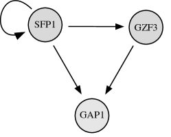
Antoneli et al. [6] employ the theory for input-output networks explained before to deal with infinitesimal homeostasis in general gene regulatory networks (GRN). As we will explain in a moment a GRN is not exactly a biochemical network as in [115]. There is a ‘mismatch’ between the number of nodes in the network and the number of state variables of the underlying system of ODEs. In order to resolve this ‘mismatch’, we generalize the approach of [7], used to analyze feedforward loops, to arbitrary GRNs. The idea there was to replace each ‘gene’ node of a GRN by a pair of ‘protein’ and ‘mRNA’ nodes to obtain a protein-mRNA network (PRN). Now, PRNs have a mathematical structure similar to that of biochemical networks and hence the theory of [134, 40] can be readily applied. More importantly, since the classification results have a purely combinatorial side, we can consider the GRN and its associated PRN simultaneously, and work out a correspondence between the classifications of homeostasis types and homeostasis patterns in both of them. Even though infinitesimal homeostasis only makes sense on the PRN (dynamical) level, its purely combinatorial aspects can be transferred to the GRN.
The main result of [6] is a complete characterization of homeostasis types and homeostasis patterns on the PRN that have correspondent on the GRN. A byproduct of this characterization is the discovery of homeostasis types and homeostasis patterns on the PRN that do not have counterparts on the GRN. The novelty of the approach of [6] is the simultaneous use of two networks, the GRN and the PRN, in the analysis of gene expression homeostasis, and the lack of assumptions about the functional form of the differential equations.
At the abstract level a GRN is a directed graph whose nodes are the genes and a directed link from a source gene to a target gene indicates that the gene product of the source gene acts as a molecular regulator of the target gene. Autoregulation occurs when a link connects a gene to itself, that is, the gene product is a molecular regulator of the gene itself.
At the dynamical level, a gene (a node in the GRN) represents the collection of processes that ultimately lead to the making of the gene product. A protein-coding gene should have at least two processes: (i) transcription, that is, the synthesis of a mRNA copy from a DNA strand and (ii) translation, that is, the synthesis of protein from a mRNA. The ‘output’ of the corresponding node in the GRN is the protein concentration at a given time.
Lut us assume the simplest scenario, namely, a GRN containing only protein-coding genes. Then, each gene (node) represents two concentrations (the concentration of mRNA and the concentration of protein). That is, there is a mismatch between the number of nodes and the number of state variables . There are two ways to deal with this mismatch.
-
[(1)]
-
1.
Protein-protein formalism. This approach is based on the fact that, in some cases, the changes to mRNA concentrations occur much faster than the changes to the concentrations of the associated proteins [111]. More specifically, the mRNA concentration quickly reaches a steady-state value before any protein is translated from it. Formally, this technique is called quasi steady-state approximation (QSSA) [123]. Then, we can solve the steady-state mRNA equations and plug the result in the protein equations. This procedure effectively reduces the number of state variables by half, thus matching of the number of nodes in the GRN (see [78, 114, 113, 120]).
-
2.
Protein-mRNA formalism. In this approach we keep the mRNA and protein concentrations for each gene and double the number of nodes of the network, leading to the notion of protein-mRNA network (PRN) [111, 91]. Now the network has two ‘types’ of nodes (mRNA and protein) and two ‘types’ of arrows (mRNA protein and protein mRNA). As we will see below there is a correspondence between the two networks that allows us to transfer some properties back and forth. For instance, this is the approach adopted in Antoneli et al. [7] for the particular example of the feedforward loop motif (see also [71]).
There are mathematical and biological reasons to prefer the second possibility. From the mathematical point of view it is more convenient to work with the PRN [94]. More specifically, it allows us to use the general theory of network dynamics [56] to associate a natural class of ODEs to a PRN, which contains virtually all models discussed in the literature. Moreover, it makes it possible to apply the techniques developed in Wang et al. [134] and Duncan et al. [40] to classify the homeostasis types in PRN and GRN.
Biologically, the use of protein-protein networks is more appropriate to model prokaryotic gene regulation, because: (i) transcription and translation occur, almost simultaneously, within the cytoplasm of a cell due to the lack of a defined nucleus, (ii) the coding regions typically take up of the genome, whereas the remaining does not encode proteins, but most of it still has some biological function (e.g., genes for transfer RNA and ribosomal RNA). In this case, it is reasonable to assume that gene expression is regulated primarily at the transcriptional level. On the other hand, gene expression in eukaryotes is a much more complicated process, with several intermediate steps: transcription occurs in the nucleus, where mRNA is processed, modified and transported, and translation can occur in a variety of regions of the cell. In particular, several non-coding genes that are transcribed into functional non-coding RNA molecules, such as, microRNAs (miRNAs), short interfering RNAs (siRNAs) and long non-coding RNAs (lncRNAs), play an important role in eukaryotic gene regulation. As we will explain later, it is very easy to incorporate these regulatory elements into the framework of PRNs (see Remark 4.10). For the moment we make the simplifying assumption that the GRN consists of protein-coding genes with transcription and translation.
Since we are interested in gene expression homeostasis, we consider input-output GRNs. They are supplied with an external parameter – e.g., environmental disturbance or transcription activity (a function of the concentration of transcription factors) – that affects the mRNA transcription of one gene, called the input gene of the GRN. The protein concentration of a second gene, called the output gene of the GRN, is the concentration where we expect to exhibit homeostasis. These two distinguished nodes are fixed throughout the analysis. We assume that only the input node is affected by the external parameter .
Definition 4.1.
Let be an input-output GRN. We define the associated PRN as follows.
-
[(a)]
-
1.
Every node in the GRN corresponds to two nodes in the associated PRN : (the mRNA concentration of gene ) and (the protein concentration of gene ). Since there is no intermediary process, the protein concentration is affected only by the mRNA concentration .
-
2.
There is a PRN arrow from and no other PRN arrow has head node . In addition, each GRN arrow leads to a PRN arrow from the protein concentration to the mRNA concentration (that is, is a transcription factor of ). Note that each arrow in the GRN leads to a single arrow in the PRN. In particular, autoregulation in leads to an arrow of .
-
3.
Finally, if the GRN has an input gene and output gene , then the associated PRN is an input-output network with input node and output node .
In particular, a PRN is always a bipartite digraph (directed graph) (see [109]), where the two distinguished subsets of nodes are the nodes and the nodes.
For example, the abstract GRN corresponding to the feedforward loop motif shown in Figure 15 is the -node input-output network shown in Figure 16(a). Its associated PRN is the -node input-output network shown in Figure 16(b).


In general, the special bipartite structure of the PRN imposes restrictions on the functional form of the admissible vector fields. For each gene there is a pair of of PRN nodes , that yields a pair of -dimensional state variables and corresponding differential equations have the form
| (4.50) |
Here, and are smooth functions. The variables are the transcription factors (TFs), that is, the corresponding protein concentrations of the genes that regulate gene . They are determined by the GRN arrows and the corresponding PRN arrows . The presence of the variable in the function occurs if and only if gene has a self-coupling in the GRN (see Remark 4.3 below). If is the input node then the function depends explicitly on the input parameter , as well. From now on we will assume only the general form (4.50) for each protein-coding gene, since our classification results depend only on the GRN coupling structure, not on the particular form of the equations (see Remark 4.2).
Remark 4.2 (Activation and Repression).
Very often in the literature GRNs are drawn with two types of arrows: (i) to indicate that gene (more specifically, its protein) acts as an activator, or excitatory transcription factor, of gene , and (ii) to indicate that gene (more specifically, its protein) acts as a repressor, or inhibitory transcription factor, of gene . In terms of the associated differential equations this information is encoded in the -dependence of the function in (4.50). Typically, the dependence of on is defined by the so called gene input function. Well-known examples of gene input functions are the classical Michalis-Menten and Hill functions [117], and their multi-variate versions [76]. Since we do not specify the functional form of the differential equations, we will not use distinct arrow types in the GRN to indicate activation/repression of genes. However, we do employ distinct arrow types (see [33]) in the PRN to distinguish mRNA to protein () and protein to mRNA () couplings.
Remark 4.3 (Autoregulation).
Self-coupling, or autoregulation, is a peculiar feature of GRNs. It means that the gene product acts as a transcription factor of the gene itself. The dynamical interpretation of autoregulation is revealed by the associated PRN. It is a coupling from the protein node to the mRNA node of the same gene (see Figure 16). Moreover, it should be clear that the self-coupling representing autoregulation is not the same as ‘self-interaction’. In fact, all nodes of the PRN are self-interacting, in the sense that the right-hand side of each differential equation explicitly depends on the state variable on the left-hand side. The clarification of the dynamical interpretation of autoregulation is another advantage of the PRN formalism.
Another simple network motif is shown in Figure 17(a). Figure 17(b) shows the associated PRN. It is called feedback inhibition and it plays an important role in the GRN of E. coli. Feedback inhibition appears twice in the regulatory cascade of carbohydrate catabolism of E. coli [96, Figs. 1 and 2(a)], with and .


Antoneli et al. [6] show that it is straightforward to use the PRN construction together with the theory of [134] to obtain all the possible homeostasis types and corresponding homeostasis patterns on the PRN. Now it remains to explain how the results obtained for the PRN can be ‘lifted back’ to the GRN. In other words, we first need to define what it means for a node in a GRN to be homeostatic. Then, we use the general theory to determine in a purely combinatorial fashion, the ‘formal homeostasis subnetworks’ of the GRN. Lastly, we show how the homeostasis subnetworks of the GRN and the associated PRN relate to each other. Since only the homeostasis subnetworks of the PRN have a ‘dynamical’ interpretation of infinitesimal homeostasis, we use the relation obtained before reinterpreting infinitesimal homeostasis on the GRN level.
Definition 4.4.
Let be a GRN with associated PRN . Let be a node with be the mRNA node and be the protein node.
-
[(a)]
-
1.
An appendage node is a single appendage node if is an appendage subnetwork of with no self-coupling.
-
2.
If is an appendage subnetwork of then it is called -null-degradation.
-
3.
If is an appendage subnetwork of then it is called -null-degradation.
-
4.
If is a structural subnetwork of then it is called -Haldane.
Now we state the first main result of [6], regarding the relation between the homeostasis subnetworks of a GRN and its associated PRN.
Theorem 4.5 ([6, Theorem 2.5]).
The homeostasis subnetworks of a GRN and its associated PRN correspond uniquely to each other, except in the following cases:
-
[(a)]
-
1.
The -Haldane subnetworks of correspond uniquely to the super-simple nodes of (super-simple nodes are not homeostasis subnetworks of ).
-
2.
For every single appendage node the appendage subnetwork of yields 2 appendage subnetworks (-null-degradation) and (-null-degradation) of .
Now we consider the following question: Can we combinatorially determine the homeostasis patterns of a GRN and its associated PRN? In principle this can be done since the classification of homeostasis patterns is purely combinatorial. We start by introducing the notion of a homeostasis pattern in a GRN that is derived from the associated PRN.
Definition 4.7.
Consider a GRN and its associated PRN . Suppose that infinitesimal homeostasis occurs in the PRN at . A node is said to be GRN-homeostatic if both associated PRN-nodes and are simultaneously homeostatic at . A GRN-generating homeostasis pattern is a homeostasis pattern on such that, for every PRN-node in corresponds to GRN-homeostatic node.
In a GRN-generating homeostasis pattern all PRN-nodes appear in mRNA-protein pairs. That is, the set of GRN-homeostatic nodes match perfectly the PRN homeostasis pattern. It is useful to introduce the following terminology. Let be a homeostasis subnetwork of the GRN . Then we define a map from the set of homeostasis subnetworks of to the set of homeostasis subnetworks of the associated as follows. If , where is a single appendage node, the is the unique subnetwork given by Theorem 4.5. If , where is a single appendage node, then . With this definition, the map is injective and the complement of its image in the set of homeostasis subnetworks of the PRN is exactly the set of -Haldane and -null-degradation subnetworks.
Theorem 4.8 ([6, Theorem 2.7]).
Let be a GRN and its associated PRN. Then the homeostasis patterns on correspond exactly to the GRN-generating homeostasis patterns on . The homeostasis patterns on associated to the -Haldane and the -null-degradation subnetworks do not correspond to homeostasis patterns on .
Remark 4.10 (Non-coding genes).
As mentioned before, in eukaryotic cells there are several regulatory mechanisms modulating transcription and translation. Almost all regulatory modulation is performed by non-coding genes, i.e., genes that are transcribed into RNA, but the RNA is not translated into protein. The PRN formalism can be extended to include non-coding genes thanks to the following observation: the gene product of a non-coding gene is an mRNA whose regulatory activity is performed by direct interaction with other mRNAs [121, 86]. Thus, unlike a protein-coding gene, a non-coding gene yields only one scalar state variable and one differential equation
Here, is a smooth function. The variables are the protein concentrations associated to the transcription factors (TFs) that regulate gene . The variables are the mRNA concentrations associated to the protein-coding genes that interact with . Finally, for each above, the corresponding mRNA equation must now depend on :
The consequence for the PRN diagram is that a non-coding gene: (i) gives rise to a single PRN-node , instead of two, (ii) receives arrows from protein nodes , (iii) has a bidirectional connection with the mRNA nodes that it interacts with . With these new requirements the PRN is no longer a bipartite digraph, now it is a tripartite digraph.
An interesting byproduct of the approach expounded above is the discovery of homeostasis types and homeostasis patterns on the PRN without GRN counterpart. The ‘new’ PRN homeostasis types are degree one homeostasis types, namely, they are related to one dimensional irreducible factors of the homeostasis determinant. They are: (i) -Haldane, that occurs when the linearized coupling between the mRNA and protein of the same gene changes from excitation to inhibition as the input parameter varies, and (ii) -null-degradation, that occurs when the linearized self-interaction of a protein changes from degradation to production as the input parameter varies. Although the existence of -Haldane and -null-degradation is mathematically established, their occurrence in biological models is unlikely. -Haldane homeostasis is related to the synthesis rate of the protein from the mRNA template and -null-degradation is related to the degradation rate of the protein. Both these rates are constant (the first is positive and the second is negative) in specific model equations for GRN modeling [111, 91].
Generally speaking, all model equations for gene expression found in the literature have an explicit functional form [7, 71, 111, 91]. Here, we assume only the general form 4.50, forced by the admissibility of vector fields with respect to the PRN. Hence, our classification results apply to virtually any model equation for gene expression. Even more importantly, this leaves open the possibility to use ‘higher-order’ terms to model more complicated interactions [19]. In the terminology of [56] our results are called model independent. This means that the classification results obtained here provide a complete list of possible behaviors, with respect to homeostasis, that is independent of the model equations – the list depends only on the topology of the network. Which of those behaviors will be observed in a particular realization of the dynamics (e.g., a model equation) depends on the specific form of the dynamics.
4.2 Intracellular Metal Ion Regulation
Metal ions such as iron, copper, zinc, calcium, etc. are involved in many crucial biological processes and are necessary for the survival of all living organisms. They are ubiquitously found in all organisms, nearly exclusively as constituents of proteins, including enzymes, storage proteins and transcription factors [68]. Due to the unique redox potential of some of these transition metals, many serve important roles as co-factors in enzymes and it is estimated that 30%-45% of known enzymes are metalloproteins whose functions require a metal co-factor [84]. However, transition metals are toxic at high intracellular concentrations, as they perturb the cellular redox potential and produce highly reactive hydroxyl radicals. Therefore, all organisms require mechanisms for sensing small fluctuations in metal levels to maintain a controlled balance of uptake, efflux, and sequestration and to ensure that metal availability is in accordance with physiological needs.
The key task of an intracellular metal homeostasis regulatory mechanism is to tightly control the concentration level of the metal, namely, the collection of weakly bound metal ion in the cell, which is available for a variety of interactions with other molecules. Cells have available mechanisms to import metal from the circulation to increase the saturation level, sequester metal using a storage protein, or exporting it through an efflux pump in order to decrease the saturation level.
In the following, we describe two published mathematical models for intracellular metal ion homeostasis, calcium and zinc, that exhibit the interesting characteristic that in the corresponding network, the input node is the same as the output node.
4.2.1 Copper
Copper is an inorganic element essential to many physiological process, including neurotransmission, gastrointestinal uptake, lactation, transport to the developing brain and growth. However, its concentration must be tightly regulated, as intracellular copper excess is associated to cellular damage and protein folding disorders [88, 75]. In addition to cytosolic copper concentration, copper in intramitochondrial space must be also strictly regulated, as it is paramount for the function of copper dependent enzymes, but it may cause oxidative stress in excessive levels [13].
Expanding briefly on the physiological implications of defective copper regulation, anomalies in the ATP7B gene generate a disorder known as Wilson disease (WD), in which dysfunctional ATP7B proteins implicate WD carriers to accumulate abnormal levels of copper in the liver and in the brain [73]. Variations in the ATP7A gene result in dysfunctional ATP7A proteins that cause three separate illnesses: Menkes disease, a severe early-onset neuro-degenerative condition in which carriers usually die by 3 years of age [72]; occipital horn syndrome, a connective disorder with typical skeleton deformations which is also clinically resembling to Menkes disease, while less aggressive in its neurological manifestation [74]; and a recently found distal motor neuropathy, marked by frequent onset at adulthood and with no apparent signs of copper metabolic abnormalities, although still poorly studied [79, 137].
A simplified version of the intracellular copper regulation mechanism was proposed in [3]. We will consider the minimal model obtained from the full model of [3]. The minimal model considers the concentration of cytosolic copper and and the trans-Golgi copper and its interaction with the metallochaperone . The ATOX1 protein takes the cytosolic copper to the Cu-ATPases ATP7A and ATP7B, which use ATP to pump copper ions to vesicles of the trans-Golgi network, where copper will be incorporated in Cu-dependent enzymes and secreted. This is called the secretory pathway and it is responsible for decreasing the cytosolic copper concentration. However, when cytosolic copper levels are low, ATP7A and ATP7B take copper from the trans-Golgi network and give it to ATOX1, leading to an increase on the cytosolic copper concentration [139].
The model is given by a system of four nonlinear ordinary differential equations. For convenience we represent the concentration of each component by: , and . That is, , , are state variables and the equations are:
| (4.51) | ||||
Here, the constants , , , , , are positive parameters and and are Hill-type functions (for ):
The quantity of interest to be controlled is the cytosolic copper concentration () There is one external input parameter representing the (normalized) concentration of extracelullar copper. The network associated to the model equations (4.51) is shown in Figure 18.
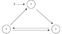
In [3] the authors show that system (4.51) has a linearly stable equilibrium and the input-output function is well-defined for all .
The general admissible system of differential equations for the network in Figure 118 is the following
| (4.52) | ||||
The jacobian at an equilibrium is
| (4.53) |
The homeostasis matrix is obtained by removing the first row and the first column, i.e.
| (4.54) |
with
| (4.55) |
Hence, for a general admissible system (4.52) it is possible to have infinitesimal homeostasis caused by the -node appendage subnetwork .
4.2.2 Calcium
In eukaryotic cells, calcium (an alkaline earth metal) functions as a ubiquitous intracellular messenger by which extracellular factors induce a variety of physiological responses. For instance, the intracellular concentration in normal yeast cell (Saccharomyces cerevisiae) is maintained in the range of 50–200 M in the presence of environmental concentrations ranging from 1 M to 100 M [100].
In [32] the authors propose a mathematical model of calcium homeostasis in normally growing yeast cells which is consistent with experimental observations available at the time of its publication.
The model is given by a system of four nonlinear ordinary differential equations. For convenience we represent the concentration of each component by: , , and . That is, are state variables and the equations are
| (4.56) | ||||
Here, , , , are positive parameters and , are sigmoid (rational) functions. The quantity of interest to be controlled is the concentration of intracellular calcium (). There is one external input parameter representing the (normalized) concentration of extracelullar calcium. The network associated to the model equations (4.56) is shown in Figure 19.
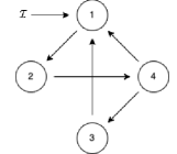
In [32] the authors show, by numerical integration, that the model equation (4.56) has an equilibrium point [32, Fig. 1a], for the parameters listed in [32, Tab. 1]. They numerically compute the input-output function of the model and plot [32, Fig. 1b] the output node variable as a function of the input parameter . The simulated cytosolic calcium concentration of the model (output node variable ) rests within 73-159 M (regardless of the initial conditions) when the simulated extracellular calcium concentration (the parameter ) ranges from 1 M to 100 M.
The general admissible system of differential equations for the network in Figure 19 is the following
| (4.57) | ||||
The jacobian at an equilibrium is
The homeostasis matrix is obtained by removing the first row and the first column, i.e.
with
Hence, for a general admissible system (4.57) it is possible to have infinitesimal homeostasis caused by null-degradation on nodes , and .
4.2.3 Zinc
Zinc is an essential micro-nutrient for plants, because it plays an important role in many enzymes catalyzing vital cellular reactions. In higher doses, however, zinc is toxic. Therefore, plants have to strictly control and adjust the uptake of zinc through their roots depending on its concentration in the surrounding soil. This is achieved by a complicated control system consisting of sensors, transmitters and zinc transporter proteins.
In [29] the authors propose a mathematical model for regulation of zinc uptake in roots of Arabidopsis thaliana based on the uptake of zinc, expression of a transporter protein and the interaction between an activator and inhibitor. The equations in [29] are obtained by an ad hoc dimensional reduction of a model proposed in [28].
The model is given by a system of four nonlinear ordinary differential equations. For convenience we represent the concentration of each component by: , , and . That is, are state variables and the equations are
| (4.58) | ||||
Here, , and are positive parameters. The quantity of interest to be controlled is the concentration of intracellular zinc (). There is one external control parameter, representing the (normalized) concentration of extracelullar zinc. The network associated to the model equations (4.58) is shown in Figure 20.
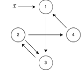
In [29] the authors show that the model equation (4.58) has a unique positive equilibrium point for any set of parameter values. They show an illustration of input-output function of the model and plot [29, Fig. 2] the output node variable as a function of the input parameter .
The general admissible system of differential equations for the network in Figure 20 is the following
| (4.59) | ||||
The jacobian at an equilibrium is
The homeostasis matrix is obtained by removing the first row and the first column, i.e.
with
Hence, for a general admissible system (4.59) it is possible to have infinitesimal homeostasis caused by null-degradation on node and the -node appendage subnetwork .
4.2.4 Iron Homeostasis
Iron is an essential component for any aerobic organism and is required for oxygen transport, cellular respiration, and many other metabolic processes. Dysregulation of iron homeostasis has been implicated in a wide variety of diseases, ranging from cancer to inflammatory and neuro-degenerative diseases. But iron is also a redox active element that can facilitate the formation of dangerous molecules, such as the hydroxyl radical, a highly reactive radical that can damage DNA, lipids, and proteins. In [27] the authors propose an explicit ODE model for the so called core control system of intracellular iron homeostasis in the form found in breast epithelial cells (see also [108]). The core control system of intracellular iron homeostasis is a regulatory network that contains several intertwined feedback loops and includes the key regulatory mechanisms of iron homeostasis. It was based on an intracellular network consisting of 151 chemical species and 107 reactions and transport steps, including cell type specific subnetworks found in [69].
The model of [27] is given by a system of five nonlinear ordinary differential equations describing changes in concentrations with respect to time for specific components of the model. We represent the concentration of each component by: , , , , and . That is, are state variables and the equations are
| (4.60) | ||||
Here, , and are positive parameters. The quantity of interest to be controlled is the liable iron pool (). There is one external input parameter the concentration level of extracelullar iron. The network associated to the model equations (4.60) is shown in Figure 21(a) (see [27, Fig. 1]), with the addition of arrows and , corresponding couplings are in the equations.
We will consider a slightly different form of this model. Since the input parameter is the amount of iron that can be transported into the cytosol, we can consider the whole term as the input to the system and discard the equation for . Moreover, since there is already a connection from node to node , the removal of node will not make it necessary to add any new link. In this case the equations become:
| (4.61) | ||||
With , , , and . Again, the quantity of interest to be controlled is the cytosolic liable iron pool (). There is one external input parameter the concentration level of extracelullar iron. The network associated to the model equations (4.60) is shown in Figure 21(b).
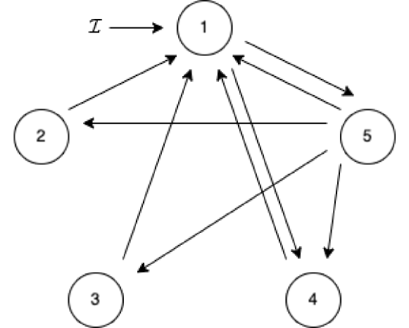
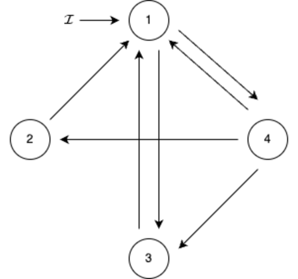
In [27] the authors show that the model equations (4.60) have a unique positive equilibrium point for any set of parameter values. They perform extensive simulations suggesting that the positive equilibrium point might be asymptotically stable in general and that (4.60) does not have limit cycle oscillations. Furthermore, they have validated the model with experimental data that show that it correctly predicts the effect of perturbing one of the network nodes on the steady state levels of two of the other nodes.
The general system of differential equations for the network in Figure 21(b) is the following
| (4.62) | ||||
The jacobian at an equilibrium is
The homeostasis matrix is obtained by removing the first row and the first column, i.e.
with
Hence, for a general admissible system (4.62) it is possible to have infinitesimal homeostasis by null-degradation on nodes , and .
4.2.5 Input=Output Networks
Antoneli et al. [5] provides a careful adaptation of the infinitesimal homeostasis formalism to the case where the input and the output nodes are the same.
When the network has the same node as the input and output nodes the corresponding variables coincide and we call the network an input=output network and the input output node.
In this case the vector of state variable is and the system of ODE’s (2.20) becomes
| (4.63) | ||||
Finally, we assume the the genericity condition (2.11), which in this case reads:
generically.
Let be the Jacobian matrix of an admissible vector field , that is,
| (4.64) |
As we have seen in the examples, the homeostasis matrix obtained from by removing the first row:
| (4.65) |
In both (4.71) and (4.65) partial derivatives are evaluated at the equilibrium .
The main difference between the homeostasis matrix (4.65) and the homeostasis matrix of network with distinct input and output nodes is that the former contains only the partial derivatives associated with the regulatory nodes, while the latter contains partial derivatives involving the input and the output nodes, as well. In fact, the matrix in eq. (4.65) is the Jacobian matrix of the subnetwork generated by the regulatory nodes.
Let us consider some small abstract networks.
Example 4.11 (-node Networks).
Trivially, there is only one network with one node. The system of ODEs associated to a one-node network is
The Jacobian is and so in order to have a stable equilibrium we must assume that . The homeostasis matrix is empty and the derivative of the input-output function is
Since we have assumed that , generically, it follows that , generically. Hence, infinitesimal homeostasis is not generically expected to occur in a one-node network.
Example 4.12 (-node Networks).
There is only one possibility, up to isomorphism, in this case: . The system of ODEs associated to this network is
The Jacobian is
and the homeostasis matrix is a scalar actually, . Hence, infinitesimal homeostasis occurs, generically, by null-degradation with respect to regulatory node .
Wang et al. [134] have shown that in order to analyze if an input-output network exhibits infinitesimal homeostasis, it is enough to study an associated “core subnetwork” (see Theorem 2.21). The same definition of core network and core-equivalence apply to an input output network and Theorem 2.21 extends to the input output case However, in the input output case, the condition that a node that is both upstream from the output node and downstream from the input node takes a special form.
Lemma 4.13.
Let be an input output network, with input output node . A regulatory node belongs to the core subnetwork if and only if belongs to a cycle that contains the input output node .
Proof 4.14.
A directed path starting and ending at the same node is a cycle.
Corollary 4.15.
An input output network is a core network if and only if every regulatory node of belongs to a cycle that contains the input output node.
In a core network where the input node is distinct from the output node, a simple node is always downstream from the input node and upstream from the output node, but not ‘the other way around’. That is, if a node is downstream the output node and/or upstream the input node then it must be an appendage node. Indeed, if is a core network the every node is downstream from the input node and upstream from the output node. Then a node that satisfies ‘the other way around’ condition above must be on an -path that cycles around the input and/or the output node. We note the not every appendage node is of this type, that is, it may be on an -path that cycles around other regulatory nodes. Hence, we have the following.
Lemma 4.16.
Let be a core input output network. Then every node of is appendage.
Proof 4.17.
Since every node in a core input output network forms a cycle with the input output node it follows that every node is downstream the output node and upstream the input node. Thus, every node is appendage. ∎
Corollary 4.18.
Structural homeostasis does not exist in input output networks.
The next theorem summarizes the classification of homeostasis subnetworks of an input output network
Theorem 4.19.
If is an input output network the the appendage subnetwork of is exactly the subnetwork of generated by all regulatory nodes. Moreover, the irreducible factors of correspond to the appendage path components and are given by . Here is the jacobian matrix associated with the network .
Proof 4.20.
By lemma 4.16 it follows that the set of nodes of is exactly the set of regulatory nodes. Hence they generate the same network. The, it follows from [134, Thm. 7.1], that all irreducible blocks of the homeostasis matrix correspond to the appendage path components. Moreover, since there are no simple nodes the “no cycle condition” is trivially satisfied by all appendage path components. Finally, it follows from [134, Thm. 5.4] that the corresponding irreducible factor of is of the form . ∎
Theorem 4.21.
Let be a directed graph. Then its condensation graph is a directed acyclic graph, i.e., has no directed cycle. Moreover, the nodes of have an acyclic ordering. That is, the path-components of can be labeled such that there is no arrow from to unless .
Proof 4.22.
See [14, pgs. 18-19 and prop. 3.1.2].
Theorem 4.21 essentially says that each component of the condensation graph represents a feedforward network. The acyclic order is a partial order on the set of nodes (the path-components of ) of the condensation graph .
The condensation graph of the appendage network of an input output network is called the condensation appendage network of . We say that a path-component is downstream from a path-component if there is a directed path from to in the condensation appendage network . A path-component is upstream from a path-component if is downstream from . We say that and not comparable if there is no directed path between them.
Theorem 4.23.
Let be an input output network and let be its appendage subnetwork. Let be the path-components of labeled according to the acyclic ordering induced by its condensation appendage network. Suppose that homeostasis is induced by . Then is induced by () if and only if is not downstream from in the condensation appendage network . In other words, if and only if
-
[(i)]
-
1.
is not in the same -path-component as .
-
2.
is not comparable to with respect to the acyclic order.
-
3.
is upstream from .
Proof 4.24.
As we have shown in Theorem 4.23, given an input output network it is possible to classify all patterns of homeostasis supported by . Moreover, each homeostasis pattern corresponds to exactly one homeostasis subnetwork.
Theorem 4.25.
Let and be two distinct homeostasis subnetworks of . Then the set of subnetworks induced by and the set of subnetworks induced by are distinct.
4.2.6 -node Input Output Networks
Now we consider the classification, up to isomorphism of the -node input output core networks.
Theorem 4.27.
There are isomorphism classes of -node input output core networks, shown in Figure 22.
Proof 4.28.
Consider the network of Figure 22(a) as a template for all other potential examples. We can see that there are possibilities for choosing the remaining arrows (A, B, C, D, E) between the three nodes , , (the arrow from to is fixed throughout the proof). The following conditions exclude a potential example: (i) the network is disconnected, (ii) the network is non-core, that is , one (or more) of the nodes does not belong to cycle with the node, and so can be removed reducing to a network with nodes. Now, the potential examples can be partitioned according to the number of additional arrows. The number of potential examples with additional arrows is . It is easy to see that and only give non-connected or non-core networks. The case corresponds to all arrows present and is a actual example, shown in Figure 22(a). The three remaining cases can be analyzed by direct inspection. See [5] for details. ∎


Theorem 4.19 implies that the kinds of homeostasis that can occur in an input output network correspond to the appendage path components. Thus it is natural to collect the isomorphism classes of networks into families according to the number of path components of the corresponding condensation appendage network.
Definition 4.29.
Define the following two families of -node input output core networks according to the number of path components of the corresponding condensation appendage network:
- Family 1:
-
the condensation appendage network has path component. In this case the appendage network is of the form and the condensation appendage network is a singleton. The -node networks of Figure 22 that belong to family 1 are: (a), (1b), (2b), (1c), (4c).
- Family 2:
-
the condensation appendage network has path components. In this case the the appendage network is of the form (subfamily 2A) or (subfamily 2B). The -node networks of Figure 22 that belong to family 2 are: (3b), (2c), (3c), (d) (subfamily 2A) and (5c) (subfamily 2B). In both cases, the condensation appendage network is equal to the appendage network and the path components are given by two singletons and .
Now we can classify the homeostasis subnetworks of the -node networks by direct application of theorem 4.19.
Theorem 4.30.
Consider a -node input output core network . Then the determinant of the homeostasis matrix is as follows:
- Family 1:
-
.
- Family 2:
-
.
That is, homeostasis in a -node input output core network is caused (i) by null-degradation on one of the two regulatory nodes or (ii) by the -node appendage subnetwork consisting of the two regulatory nodes.
Corollary 4.32.
Two -node input output core networks are core equivalent if and only their condensation appendage networks have the same number of path components.
Combining corollary 4.32 with theorem 2.29 gives a complete classification of all -node core networks, up to core equivalence.
Corollary 4.33 (All -node core networks).
There are core equivalence classes of -node input-output core networks. Representatives are given by: (i) the Feedforward Excitation motif, (ii) the Substrate Inhibition motif, (iii) the Negative Feedback motif, (iv) the -node Loop motif, Figure 22(d) and (v) the Antithetic Feedback motif, Figure 22(1c). Any other -node input-output network can be obtained from these representatives by adding and /or removing backward arrows.
Remark 4.34 (Backward arrows).
The notion of backward arrow in the input output case is more subtle. Let be an input output core network. A backward arrow in is any arrow coming into or out of the input node such that after its removal remains a core network. The problem here arises when we add and / or remove several backward arrows. The order in which the arrows are added and / or removed matters. For example, networks (1c) and (4c) in Figure 22 are core equivalent and so each one can be converted into the other by adding and /or removing backward arrows. To convert (1c) and (4c) one first adds the arrow and then removes the arrow . To convert (4c) to (1c) one first adds the arrow and then removes the arrow . In this last case, if one reverses the procedure and first removes the arrow the resulting network becomes non-core. The same happens with the first case, if one first removes the arrow the resulting network becomes non-core.
Example 4.35 (-Node Feedback Loop).
Consider the -Node Feedback Loop motif in Figure 22(d). It is the only three node input output with three arrows. The system of ODEs associated to this network is
The Jacobian is
The homeostasis matrix is
Thus
That is, infinitesimal homeostasis can occur by null-degradation with respect to regulatory nodes or .
Example 4.36 (Antithetic Feedback).
Consider the -node Loop motif in Figure 22(1c). This is the network for the copper homeostasis model. This network have been considered by several authors [21, 46, 9, 122] because of its capability to exhibit perfect homeostasis. The system of ODEs associated to this network is
The Jacobian is
The homeostasis matrix is
Thus
That is, infinitesimal homeostasis can occur by the -node appendage subnetwork . The model considered in [21, 46, 9, 122] has an additional feature that makes it capable of exhibiting perfect homeostasis. It satisfies the antithetic identities
| (4.66) |
By plugging these identities in the expression for one easily obtains
Interestingly, the model equations for copper homeostasis do not satisfy the antithetic identities (4.66). Nevertheless, it has been shown in [3] that this model can exhibit infinitesimal homeostasis.
In Example 2.28 we analyzed the Negative Feedback Loop and showed that null-degradation together with linear stability implies negative feedback between the regulatory node that causes homeostasis and the output node. It would be interesting to know if it makes sense to ask the same for the core equivalence class of the antithetic feedback, namely, is it true that appendage homeostasis together with stability implies ‘negative feedback’? The first step to answer this question would be to make it more precise what it means ‘negative feedback’ in the context of -node input output networks.
4.3 Bacterial Chemotaxis
The mathematical modeling of chemotaxis can be roughly divided into two types: single cell models and bacterial population models [131, 130]. Single cell models consider the activation of the flagellar motor by detection of attractants and repellents in the extracellular medium. The flagellar motor activity of bacteria is regulated by a signal transduction pathway, which integrates changes of environmental chemical concentrations into a behavioral response. Assuming mass-action kinetics, the reactions in the signal transduction pathway can be modeled mathematically by ODEs. The bacterial population models describe evolution of bacterial density by parabolic PDEs involving an anti-diffusion ‘chemotaxis term’ proportional to the gradient of the chemoattractant, thus allowing movement up-the-gradient, the most prominent feature of chemotaxis. The most extensively studied bacterial population models are the Patlak-Keller-Segel (PKS) type models.
Understanding the response of E. coli cells to external attractants has been the subject of experimental work and mathematical models for nearly 40 years. In fact, many models of the chemotaxis have been formulated and developed to provide a comprehensive description of the cellular processes and include details of receptor methylation, ligand-receptor binding and its subsequent effect on the biochemical signaling cascade, along with a description of motor driving CheY/CheY-P levels, the main output of the chemotaxis system (see [131] for a survey).
However, including such detail has often led to very complex mathematical models consisting of tens of governing differential equations, making mathematical analysis of the underlying cellular response difficult, if not in many cases, impossible. A model proposed by Clausznitzer et al. [30] has sought to provide a comprehensive description of the E. coli response, by coupling a simplified statistical mechanical description of receptor methylation and ligand binding, with the signaling cascade dynamics. The model consists of five nonlinear ordinary differential equations (ODEs) and is parametrized using data from the literature. The authors were able to show that the model is in good agreement with experimental findings. However, being a fifth-order nonlinear ODE model, it is difficult to treat analytically. More recently, Edgington and Tindall [43] undertook a comprehensive mathematical analysis of a number of simplified forms of the model of [30] and proposed a fourth-order reduction of this model that has been used previously in the theoretical literature [42].
In the following we shall consider the model proposed by [42, 43]. It has four variables for the concentrations of CheA/CheA-P (), CheY/CheY-P (), CheB/CheB-P () and the receptor methylation () and is given by the following system of ODEs (in non-dimensional form):
| (4.67) | ||||
where , , are non-dimensional parameters, the extracellular ligand concentration is the external parameter and the function is determined by a Monod-Wyman-Changeux (MWC) description of receptor clustering
| (4.68) |
with
| (4.69) |
The abstract input-output network obtained from system 4.67 is shown in Figure 23. Here, the variables in the original system correspond to the nodes as follows: , , , , .
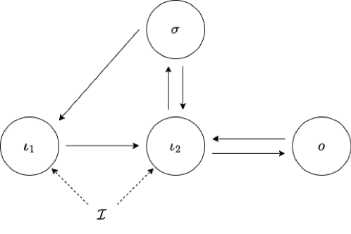
The problem here is that we cannot apply the theory of [134] to this network since it has two input nodes. The extension of the theory to this new situation has been obtained by Madeira and Antoneli [92].
The key observation of [43] is that system (4.67) has a unique asymptotically stable equilibrium
with , and positive and is a real number, for the non-dimensional parameters obtained from the parameter values originally used in [30]. Furthermore, [43] were able to show that some pairs of parameters might yield oscillatory behavior, but in regions of parameter space outside that observed experimentally. This was done by carrying out the stability analysis for pair-wise parameter variations, whereby for each case the occurrence of at least two non-zero imaginary parts was recorded as indicating possible oscillatory dynamics. The steady-state can be easily found by numerical integration for parameter values that are experimentally valid, although some combinations of parameters produce a large stiffness coefficient [30].
More importantly, the stability of persists as is varied in the range . By standard arguments this implies that there is a well-defined smooth mapping . Since the values of , and are independent of (see [43]), it follows that the individual component functions , and are actually constant functions with respect to .
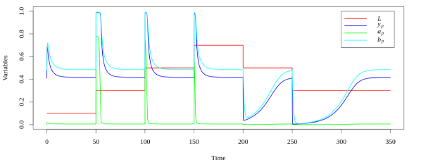
In Figure 24 we show the time series of the three variables , and and how they are perturbed when the parameter is varied by sudden jumps. After a transient, which depends on the contraction rates at the equilibrium point, each variable returns to its corresponding steady-state value. Moreover, when the parameters , , are changed the equilibrium also changes, but the new functions , and remain constant with respect to , possibly with different values. This is exactly the robust perfect homeostasis that was shown to occur in other models of chemotaxis [15, 1, 97, 138, 85, 65].
4.3.1 Multiple input-node networks
A multiple input-node input-output network is a network with distinguished input nodes , all of them associated to the same input parameter , one distinguished output node , and regulatory nodes . Here, we explicitly assume that the output node is distinct from all the input nodes. The associated network systems of differential equations have the form
| (4.70) | ||||
where is an external input parameter and is the vector of state variables associated to the network nodes.
An admissible vector field associated with the system (4.70) can be witten as
Finally, we assume the genericity condition (2.11), which in this case reads
generically, for all .
Let be the Jacobian matrix of an admissible vector field , that is,
| (4.71) |
The matrix obtained from by replacing the last column by , is called generalized homeostasis matrix:
| (4.72) |
Here all partial derivatives are evaluated at .
Lemma 4.37.
The input-output function satisfies
| (4.73) |
Here, and are evaluated at . Thus, is a point of infinitesimal homeostasis if and only if
| (4.74) |
at the equilibrium .
Proof 4.38.
The notion of core network can be extended to the multiple input node context and a similar result to theorem 2.21 holds [92, Thm. 3.2].
By expanding with respect to the last column and each (input) row one obtains
| (4.76) |
Note that when there is a single input node, i.e. , Lemma 4.37 gives the corresponding result obtained in [134]. In this case, there is only one matrix , the homeostasis matrix, that played a fundamental role in the theory developed in [134]. Hence, it is expected that the matrices should play a similar role in the generalization of [134] to the multiple input node case.
Definition 4.39.
Let be an input-output network with input nodes and be an admissible vector field. The partial homeostasis matrix of is obtained from the Jacobian matrix of by dropping the last column and the row
| (4.77) |
When the network has only one input node, eq. (4.77) gives exactly the homeostasis matrix defined in [134].
The classification of homeostasis types proceeds as in [134]. The first step is to apply Frobenius-König theory [118, 23] to the generalized homeostasis matrix . More precisely, Frobenius-König theory implies that there exist (constant) permutation matrices and such that
| (4.78) |
where each diagonal block , …, and is irreducible (in the sense of [23]). Hence, , …, and are irreducible polynomials. As and are constant permutation matrices, we have that
| (4.79) |
In order to simplify nomenclature, we will call , …, and irreducible homeostasis blocks, although in the literature the term irreducible matrix may have a different meaning (see [118]).
A direct comparison of factorization (4.79) with expansion (4.76) suggests that the irreducible factors are the common factors of and is a weighted alternating sum of . Indeed, as we show in [92] the matrix in (4.78) contains all the functions as entries, that is, it is a homogeneous polynomial of degree on , whereas the matrices do not contain any of them.
The next step is to classify the irreducible homeostasis blocks of according to their number of self-couplings. Indeed, we show that each block of order has exactly or self-couplings [92, Sec. 3.4]. But, unlike [134], in the multiple input nodes case we find three classes (instead of two classes) of irreducible homeostasis blocks that may occur in core networks with multiple input nodes.
Definition 4.40.
Let be an irreducible homeostasis block of order that does not contain any partial derivatives with respect to . The homeostasis class of is appendage if has self-couplings and structural if has self-couplings.
Definition 4.41.
The network exhibits appendage homeostasis if there is an appendage irreducible homeostasis block such that . In an analogous way, exhibits structural homeostasis if there is a structural irreducible homeostasis block such that .
As shown in [134], appendage and structural homeostasis occur in core networks with one input node. Nevertheless, networks with multiple input nodes also exhibit a new class of homeostasis that is not found in networks with only one input node.
Definition 4.42.
Let be an irreducible homeostasis block whose determinant is a homogeneous polynomial of degree on the variables . We say that the homeostasis class of is input counterweight. Moreover, we say that exhibits input counterweight homeostasis when .
Although input counterweight homeostasis does not occur in networks with only one input node, it is interesting to note that in these networks there is a corresponding matrix . In fact, from equation (4.72) and considering networks with only one input node , we have
| (4.80) |
As, by hypothesis, , the input counterweight homeostasis is never present in networks with only one input node. On the other hand, the block can always vanish in any network with more than one input node [92, Cor. 3.9].
The final step in this theory is to identify a homeostasis subnetwork of corresponding to each homeostasis block of in such a way that each class of homeostasis corresponds to a distinguished class of subnetworks. Because of the appearance of a third homeostasis class, the extension of the results of [134] to the multiple input nodes is not a trivial extension. See [92] for more details.
4.3.2 The E. coli Model
Since the network corresponding to the model equations 4.67 has two input nodes it cannot be analyzed using the methods of [134]. In fact this can be seen directly from the equations 4.67, since both the equation for and depend on the external parameter .
In order to apply the theory developed in [92] to the model for the Escherichia coli chemotaxis of [43], we first rewrite the system (4.67) in the standard form (4.70). Using the correspondence between variables defined before, we obtain the following system of ODEs
| (4.81) | ||||
with the function given by (4.68) and input parameter . The ODE system (4.81) is an admissible system for the abstract input-output network shown in Figure 23. In fact, the general form of an admissible system for this network is
| (4.82) | ||||
From the theory developed in this paper, it is clear that the network is a core network with input nodes and and output node . The Jacobian matrix of network is:
| (4.83) |
The generalised homeostasis matrix of network is:
| (4.84) |
It can be decomposed as
| (4.85) |
where
and
Hence, the complete factorization of is
Summarizing, network (Figure 23) generically supports three types of homeostasis: (1) appendage (null-degradation) homeostasis associated with the subnetwork , (2) structural (Haldane) homeostasis associated with the subnetwork and (3) input counterweight homeostasis associated with the subnetwork . See [92] for a more conceptual derivation of the determinant using only the topology of the network.
Now, specializing to the model equations (4.81), we observe that, although the abstract network supports appendage and structural homeostasis, the model equations (4.81) cannot exhibit these types of homeostasis. In fact, at equilibrium we have that
| (4.86) |
and
| (4.87) |
The first inequality follows because all parameters are positive and is positive at equilibrium. The last inequality follows because , at equilibrium, so one would have .
This leaves the only remaining possibility: input counterweight homeostasis. To verify that the model equations (4.81) indeed exhibit input counterweight homeostasis we compute, assuming that both and are non-zero:
| (4.88) | ||||
Thus, for any function , we have
| (4.89) |
In particular, and so the model equations (4.81) exhibits, not only infinitesimal homeostasis (of the input counterweight type), but perfect homeostasis.
Moreover, it is easy to check that in the model equations (4.81), both and are non-zero. Hence, all the partial derivatives of in (4.88) are non-zero and so the occurrence of perfect homeostasis in this model is non-trivial. Figure 25 (bottom-left) shows the graph of the output variable (blue) as a function of the parameter . As expected, it is a constant line over the whole range of .
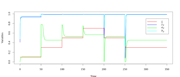
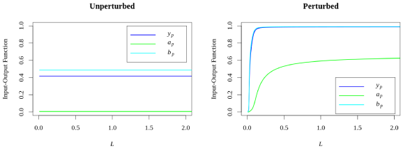
A consequence of the above calculation is that the property of perfect homeostasis in the model (4.81) for E. coli chemotaxis is persistent, in the sense that it does not depend on the values of the parameters of the model. Even more, its persistence holds for a much larger set of perturbations than just parameter variation, since there is a functional dependence in the input-output function (see [92] for the details).
As can be seen in Figure 24 it looks like the time series of all three variables , and exhibit perfect homeostatic behavior. This is the homeostasis pattern associated with homeostasis type the caused homeostasis. A theory of homeostasis patterns for networks with multiple input nodes has not been worked yet and thus we cannot predict the homeostasis patterns from the knowledge of the homeostasis types alone. The only way to determine the homeostasis patterns in this case is by numerical computation.
As we have seen, there is a symmetry between the two first equations of (4.81) that cause the identical vanishing of the determinant . Therefore, it is reasonable to think that in order for a perturbation to disrupt the perfect homeostasis it is necessary that the perturbation breaks the symmetry above. Consider the -parameter family of perturbations of (4.81)
| (4.90) | ||||
where and is a fixed smooth function. It is clear that (4.90) is admissible for the network for all and any smooth function . Moreover, (4.90) reduces to (4.81) when . The expressions for , and are independent of and thus are the same as in the original system (4.88). The expression for now is
| (4.91) |
Since the equations of and of are independent of , the same argument as before shows that system (4.90) does not exhibit appendage or structural homeostasis, for all . Now to show that the input counterweight homeostasis factor cannot be identically zero we compute
Since and , generically, left-handed side vanishes if vanishes, generically
Therefore, if the function does not vanish on an interval (say, ), system (4.90) does not exhibit perfect homeostasis, generically, for .
Nevertheless, it is still possible that (4.90) exhibits infinitesimal homeostasis. In fact, the function determines the critical points of the input counterweight factor. That is, at some if
In particular, if has a critical point at , or equivalently, if vanishes on , then is a point of infinitesimal homeostasis.
More generally, numerical simulations suggests that, when is small, system (4.90) displays near perfect homeostasis, see Figure 25 (bottom-right).
Finally, we should mention that another extension of the theory of [134] to the case of multiple input nodes and multiple input parameters has been developed [93]. Thus, one can apply essentially the same combinatorial tools to study homeostasis in any MISO system given in terms on an input-output network.
4.4 Period Homeostasis and Circadian Rhythms
Circadian clocks are endogenous oscillators that are prevalent in organisms from bacteria to humans and control -hour physiological and behavioral processes in these organisms. Such oscillations are thought to work as pacemakers, and the maintenance of their characteristic period to a constant value against changes in external conditions is important. To date, it is known that some of these oscillators display ‘period homeostasis’ against external changes [16]. The most prominent example of period homeostasis is called temperature compensation, i.e., persistence of the period against temperature changes [66]. In addition to temperature compensation, circadian clocks display persistence against changes in trophic conditions, which is called nutrient compensation [110]. Such homeostatic features (i.e., temperature and nutrient compensation) are known to be universally conserved across a wide range of organisms [67].
The mammalian circadian system is composed of a hierarchical multi-oscillator structure, with the central clock located in the suprachiasmatic nucleus (SCN) of the hypothalamus regulating the peripheral clocks found throughout the body. At the cellular level, each cell is governed by its own independent clock; and yet, these cellular circadian clocks in the SCN form regional oscillators that are further coupled to one another to generate a single rhythm for the tissue. The oscillatory coupling within and between the regional oscillators appears to be critical for the extraordinary stability and the wide range of adaptability of the circadian clock [35].
In the past two decades, key clock genes have been discovered in mammals and shown to be interlocked in transcriptional and translational feedback loops. Interestingly, the mammalian circadian clock also seems to be persistent to global changes in transcription rates and gene dosage [34].
To investigate the dynamics and mechanisms of the intracellular feedback loops in circadian clocks, a number of mathematical models based on systems of ordinary differential equations have been developed. The majority of models use Hill functions to describe transcriptional repression in a way similar to the Goodwin model [82].
In order to understand what period homeostasis means in these models let us consider a parametrized system of ODEs as in 2.1 with for simplicity. But now we suppose that is a stable periodic solution of (2.1) with minimal period .
By the continuation of hyperbolic periodic solutions theorem [64, Thm. 1.1], there is a smooth family of periodic solutions defined in a neighborhood of , with smooth minimal period , such that , and for all .
There are several proofs of this theorem, mostly often using the method of Poincaré sections. Hale and Raugel [64] considers a simple method using the Fredholm alternative and the Lyapunov-Schmidt procedure.
Let us call the mapping the period input-output function. Then we can adapt Definition 2.1 to give a notion of infinitesimal period homeostasis.
Definition 4.43.
Let be the period input-output function. We say that exhibits infinitesimal period homeostasis at the point if
| (4.92) |
That is, is a critical point of the the period input-output function .
Of course one can easily formulate analog definitions for perfect period homeostasis and near-perfect period homeostasis. Accordingly, we will refrain from writing down these definitions.
Furthermore, it is possible to adapt the proof the continuation theorem given in [64] to obtain an explicit formula for the derivative of . Let be fixed and set and
| (4.93) |
where is the unique solution of the adjoint Floquet operator of the solution , with periodic boundary condition and the normalization condition . Here, is the standard scalar product on .
The adjoint Floquet operator of the solution is defined as follows. Let be the linearization of about the periodic solution , then is a -periodic function. Then and are the Floquet operator and the adjoint Floquet operator of the solution , respectively. See also [141], where the function is called infinitesimal phase response curve (iPRC) of the periodic solution .
Now that we have a precise notion of period homeostasis and a means to compute it we could try to apply it to some example. Although, formula (4.93) is quite nice conceptually, it seems very hard to compute in concrete examples. An alternative is to use numerical methods for continuation periodic solutions, such as Auto from XPPAut [44]. We will illustrate this idea of numerical continuation periodic solutions with a simple model for the mammalian circadian system.
Example 4.44 (Mammalian Clock Model).
Kim and Forger [83] propose to use a mechanism of protein sequestration-based (PS) transcriptional repression rather than Hill-type (HT) repression. Since Goodwin’s and Goldbeter’s pioneering studies, Hill functions have been widely used to model the negative feedback loops (NFL) in circadian clocks of diverse organisms, including Neurospora, Drosophila and mammals [82]. In [83] the authors formulate three simple mathematical models for the mammalian clock (based on a more detailed model), that reproduces a surprising amount of experimental data on mammalian circadian rhythms. See also Yao et al. [136] for a careful mathematical analysis.
The Simple Negative Feedback (SNF) loop model is generated by modifying the well-studied Goodwin model to include an activator, which can be inactivated when bound in complex with the repressor. The state variables are: the mRNA concentration (), the cytoplasmic protein concentration () and the nucleous protein concentration . The mRNA transcription is proportional to the % of unbound free activator , which indicates the activity of the promoter. Here, the parameter is the upstream transcriptional factor that interacts with through binding with dissociation constant . That is, the transcription of the mRNA is repressed by by inhibition of the activator See [83, 136] for details.
The other two models can be obtained from the SNF through the addition of negative or positive feedback loops controlling the production of activator , which then becomes another state variable. The Positive-Negative Feedback (PNF) loop model and the Negative-Negative Feedback (NNF) loop mode are obtained from the (SNF) adding two state variables: is the protein that activates the transcription of and is the mRNA the is associated to protein . See [83, 136] for details.
It is possible to write down the non-dimensional equations for the three models at same time
| (4.94) |
where
and , , , , , , , , , , are parameters.
The SNF model is obtained by setting . Then the equations for and disappear and becomes another parameter. The PNF model is given by picking the positive () exponent in on the right-handed side of the equation for and the NNF model is given by picking the negative () exponent in on the right-handed side of the equation for .
It is shown in [83] that the three models have stable periodic solutions for a large range of the parameters. See also [136] for an analysis of the Hopf bifurcation that generates these solutions.
In Figure 26 we show numerical computation of the period input-output function for the three models. In the SNF model we use as the input parameter and the PNF and NNF models we use as the input parameter. The output is the period of the periodic solution in all three cases.
In all three cases we see that the period input-output function has an infinitesimal homeostasis point at the left end of each curve and exhibits near-perfect homeostasis at the right end of the graph. Moreover, in the PNF case the periodic orbit undergoes a saddle-node bifurcation.
r8ptt9pt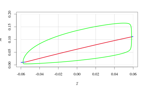
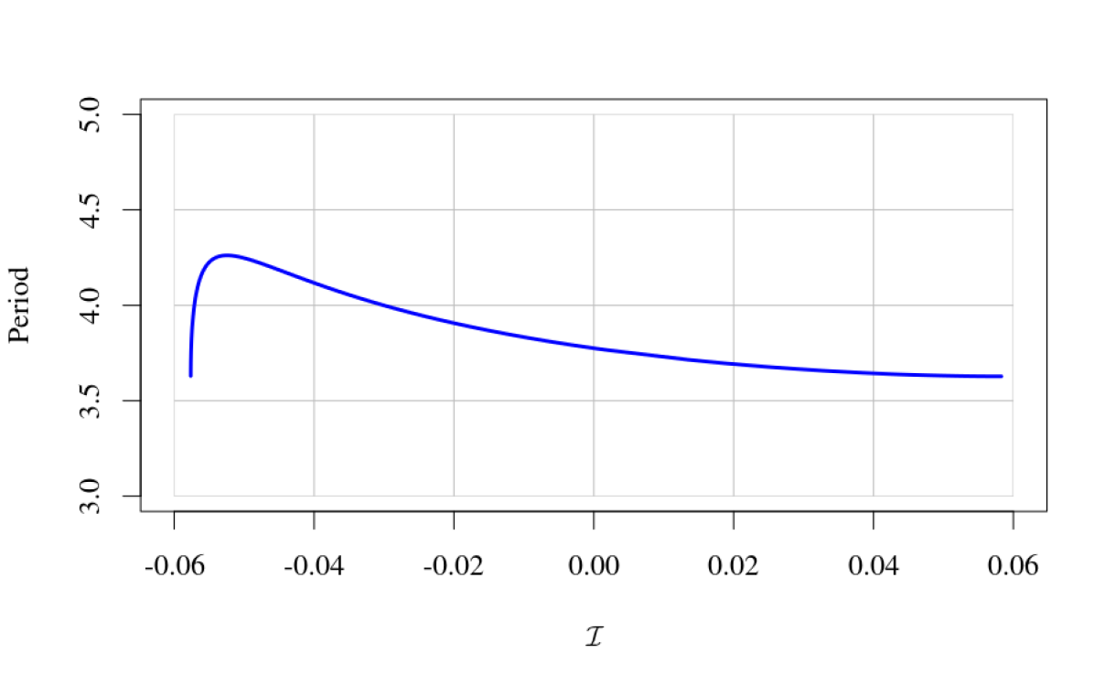
r8ptt9pt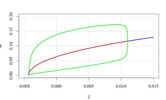
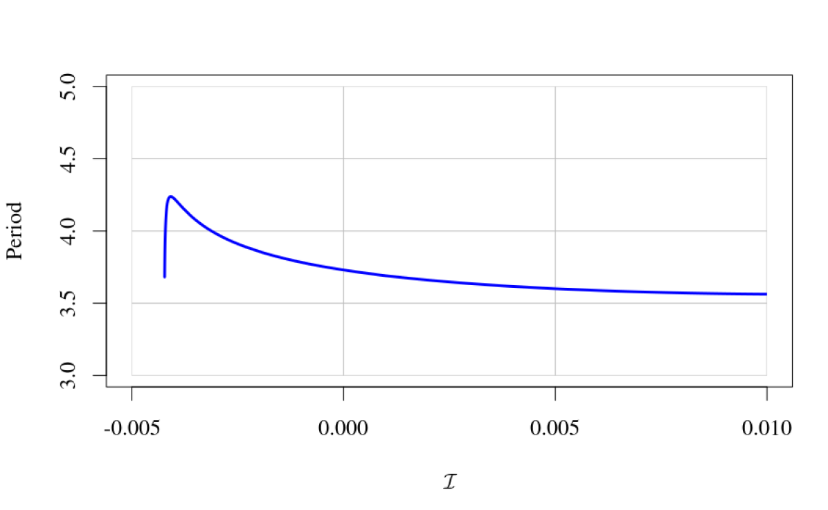
r8ptt9pt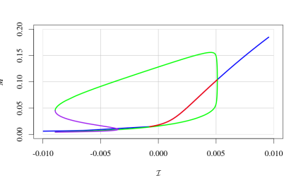
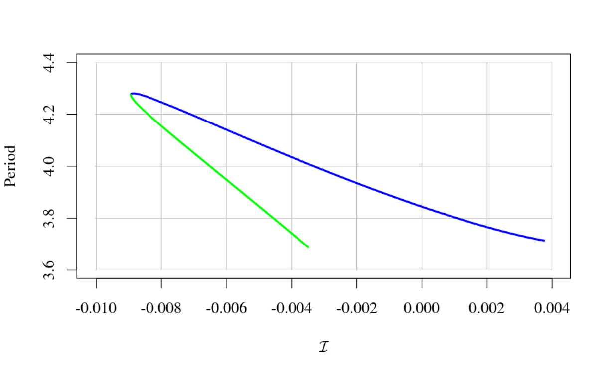
Notwithstanding its biological relevance, period homeostasis seems to be quite different from the steady-state homeostasis studied before. For instance, it does not need a network structure or an observable on the state space to be defined.
However, it is possible to define a notion of homeostasis associated with periodic orbits that is analogous to the steady-state theory. Motivated by problems in neuroscience Yu and Thomas [141] provided the first step towards such a theory by introducing a new class of input-output functions.
Yu and Thomas [141] start, as before, with a parametrized system of ODEs as in 2.1 possessing a stable periodic solution with minimal period and consider its continuation defined in a neighborhood of , with smooth minimal period , such that , and for all . Now, given a smooth observable defined on the state space consider the input-output function given by averaging along
| (4.95) |
Note that the minimal period function now appears in the definition of the averaging operator.
For example, if the system of ODEs has an underlying input-output network with output node the we can define the input-output function
| (4.96) |
where is the -coordinate of . It is clear that this new class of input-output functions is provides the right counterpart in the periodic case to the steady-state input-output functions.
The main result of [141] is a formula for the derivative of the input-output function with respect to . To accomplish this they propose ageneralization of the infinitesimal shape response curve (iSRC) recently introduced in [133]. The iSRC complements the well-known infinitesimal phase response curve (iPRC). The latter quantifies, to linear order, the effect of an instantaneous perturbation on the timing of the periodic solution, and also captures the cumulative effect of a sustained perturbation its period. In contrast, the iSRC captures the effect of a sustained or parametric perturbation on the shape of the periodic solution, to linear order.
The formula for the derivative of obtained by [141] is very similar to formula (4.93) Let be fixed and set and
| (4.97) |
where is the generalized iSRC of the periodic solution [141]. That, is is a -periodic solution of an inhomogeneous linear equation similar to the adjoint Floquet operator.
The similarity with formula (2.5) is noteworthy. In both cases, the derivative is given by the scalar product (the average operation in formula (4.97) can be written as scalar product in the space of -periodic functions) between the gradient of the observable and a solution of a linear equation obtained by linearization of the parametrized family of nonlinear equations at the appropriate solutions. As we noted before, the period input-output function is an exceptional observable that do not have a counterpart in the steady-state context.
The work of [141] is an important advance in the extension of homeostasis to the periodic case. However, the theory is much less developed in relation to the steady-state case. For instance, an extension of the combinatorial structure theory for homeostasis in input-output networks with input-output functions of the from (4.96) remains elusive. Extending the classification theory to this context would be an interesting future direction.
5 Conclusion and Outlook
Undoubtedly there are many other directions for research on infinitesimal homeostasis that we have not explored in this review.
For example, we have mentioned that Duncan and Golubitsky [41] have investigated forms of combining infinitesimal homeostasis and bifurcations. In fact, there are two generalizations of homeostasis theory that are motivated by codimension arguments in bifurcation theory. The first is related to chair homeostasis, where the plateau in the input-output function is flatter than expected. See Nijhout et al. [103], Golubitsky and Stewart [55], and Reed et al. [115]. The second is related to the existence of ‘homeostasis mode interaction’, where two infinitesimal homeostasis types occur at the same equilibrium. See Duncan et al. [39]. Interestingly, the simultaneous appearance of different homeostasis types leads to bifurcation in the family of equilibria that generates the homeostasis. An early example of this phenomenon is discussed in Duncan and Golubitsky [41]. A related biochemical example of multiple types of infinitesimal homeostasis occurring on variation of just one parameter is found in Reed et al. [115].
Another line of research is the role of homeostasis in chemical reaction network theory [45, 140]. Craciun and Deshpande [31] initiated the investigation of infinitesimal homeostasis in chemical reaction networks by relating it to the notion of network injectivity. More precisely, the authors describe a procedure for checking whether a reaction network may admit infinitesimal homeostasis by constructing a modified network and checking if it is injective [31, Thm. 3.4]. They also obtain a sufficient condition for perfect homeostasis [31, Thm. 3.5]. See also [11] for the occurrence of perfect homeostasis in chemical reaction networks from a control theoretic point of view.
Finally, we should mention the possibility to extend the theory the stochastic realm. In [21, 9] the authors study the occurrence of perfect homeostasis in a stochastic version of the antithetic model (see Example 4.36 of subsection 4.2). More generally, the typical stochastic processes that are considered in [21, 9] and many other modeling approaches to biological systems are called stochastic chemical reaction networks [2].
In the stochastic setup a model is given by a continuous-time ergodic Markov process on a state space with stationary (equilibrium) measure . It is assume that the model depends on an input parameter and that the stationary measure is a function of the input parameter: . Given an observable,i.e. an integrable function , its expectation with respect to the stationary measure is
is a function of the parameter . We say that the system exhibits linear response for at if the derivative
exists. Linear response can be rigorously justified for a large class of stochastic processes [62, 90]. Taking as the input-output function, with fixed, the definitions of perfect, near-perfect and infinitesimal homeostasis readily go through this new context. Now the basic question is: Which parts of the ‘machinery’ developed for the deterministic setting (e.g. singularity structure, input-output networks and the combinatorial classification of homeostasis types, homeostasis patterns, etc.) can be extended to the stochastic version? Even more so, in the stochastic setting there are many problems and questions that have no counterpart in the deterministic setting.
Acknowledgments
We thank Janet Best, William Duncan, João Luiz Madeira, Fred Nijhout, Michael Reed, John Tyson and Yangyang Wang for helpful discussions. We thank the organizers of the Workshop “Dynamical Systems in the Life Sciences”, Harsh Jain, Wenrui Hao, Grzegorz Rempala and Yangyang Wang. The research of FA was supported by Fundação de Amparo à Pesquisa do Estado de São Paulo (FAPESP) grants 2019/21181-0 and 2023/04839-7.
References
- Alon et al. [1999] Alon, U., Surette, M.G., Barkai, N., Leibler, S., 1999. Robustness in bacterial chemotaxis. Nature 397, 168–171. doi:10.1038/16483.
- Anderson and Kurtz [2015] Anderson, D.F., Kurtz, T.G., 2015. Stochastic analysis of biochemical systems. volume 674. Springer.
- Andrade et al. [2022] Andrade, P.P.A.C., Madeira, J.L.O., Antoneli, F., 2022. Homeostatic mechanisms in biological systems. arXiv 2202.11218, 1–31. doi:10.48550/arXiv.2202.11218.
- Ang and McMillen [2013] Ang, J., McMillen, D.R., 2013. Physical constraints on biological integral control design for homeostasis and sensory adaptation. Biophysical Journal 104, 505–515.
- Antoneli et al. [2024] Antoneli, F., Best, J., Golubitsky, M., Jin, J., 2024. Homeostasis in networks with same input and output nodes and metal ion regulation. In preparation .
- Antoneli et al. [2023] Antoneli, F., Golubitsky, M., Jin, J., Stewart, I., 2023. Homeostasis in gene regulatory networks. arXiv: 2309.06509, [q–bio.MN]. doi:10.48550/arXiv.2309.06509.
- Antoneli et al. [2018] Antoneli, F., Golubitsky, M., Stewart, I., 2018. Homeostasis in a feed forward loop gene regulatory motif. Journal of Theoretical Biology 445, 103–109. doi:10.1016/j.jtbi.2018.02.026.
- Antoneli and Stewart [2022] Antoneli, F., Stewart, I., 2022. Right network-preserving diffeomorphisms. Journal of Singularities 25, 1–29.
- Aoki et al. [2019] Aoki, S.K., Lillacci, G., Gupta, A., Baumschlager, A., Schweingruber, D., Khammash, M., 2019. A universal biomolecular integral feedback controller for robust perfect adaptation. Nature 570, 533–537.
- Araujo and Liotta [2018] Araujo, R.P., Liotta, L.A., 2018. The topological requirements for robust perfect adaptation in networks of any size. Nature Communications 9, 1757.
- Araujo and Liotta [2023] Araujo, R.P., Liotta, L.A., 2023. Universal structures for adaptation in biochemical reaction networks. Nature Communications 14, 2251.
- Arnold [1976] Arnold, V.I., 1976. Local normal forms of functions. Inventiones Mathematicae 35, 87–109.
- Baker et al. [2017] Baker, Z.N., Cobine, P.A., Leary, S.C., 2017. The mitochondrion: A central architect of copper homeostasis. Metallomics: Integrated Biometal Science 9, 1501–1512.
- Bang-Jensen and Gutin [2018] Bang-Jensen, J., Gutin, G. (Eds.), 2018. Classes of Directed Graphs. Springer Monographs in Mathematics, Springer International Publishing, Cham. doi:10.1007/978-3-319-71840-8.
- Barkai and Leibler [1997] Barkai, N., Leibler, S., 1997. Robustness in simple biochemical networks. Nature 387, 913–917. doi:10.1038/43199.
- Bell-Pedersen et al. [2005] Bell-Pedersen, D., Cassone, V.M., Earnest, D.J., Golden, S.S., Hardin, P.E., Thomas, T.L., Zoran, M.J., 2005. Circadian rhythms from multiple oscillators: lessons from diverse organisms. Nature Reviews Genetics 6, 544–556.
- Bernard [1865] Bernard, C., 1865. Introduction à l’étude de la médecine expérimentale. Baillière, Paris.
- Best et al. [2009] Best, J.A., Nijhout, H.F., Reed, M.C., 2009. Homeostatic mechanisms in dopamine synthesis and release: A mathematical model. Theoretical Biology and Medical Modelling 6, 21. doi:10.1186/1742-4682-6-21.
- Bick et al. [2023] Bick, C., Gross, E., Harrington, H.A., Schaub, M.T., 2023. What are higher-order networks? SIAM Review 65, 686–731.
- Bortner et al. [2023] Bortner, C., Gross, E., Meshkat, N., Shiu, A., Sullivant, S., 2023. Identifiability of linear compartmental tree models and a general formula for input-output equations. Adv. Appl. Math. 146, 102490. URL: https://doi.org/10.1016/j.aam.2023.102490, doi:10.1016/j.aam.2023.102490.
- Briat et al. [2016] Briat, C., Gupta, A., Khammash, M., 2016. Antithetic integral feedback ensures robust perfect adaptation in noisy biomolecular networks. Cell Systems 2, 15–26.
- Bröcker and Lander [1975] Bröcker, T., Lander, L., 1975. Differentiable Germs and Catastrophes. volume 17. Cambridge University Press.
- Brualdi and Ryser [1991] Brualdi, R.A., Ryser, H.J., 1991. Combinatorial Matrix Theory. Cambridge University Press.
- Cannon [1929] Cannon, W.B., 1929. Organization for physiological homeostasis. Physiological reviews 9, 399–431.
- Cannon [1939] Cannon, W.B., 1939. The wisdom of the body. Norton & Co.
- Castrigiano and Hayes [2004] Castrigiano, D., Hayes, S., 2004. Catastrophe Theory: Second Edition. The Advanced Book Program, Avalon Publishing.
- Chifman et al. [2012] Chifman, J., Kniss, A., Neupane, P., Williams, I., Leung, B., Deng, Z., Mendes, P., Hower, V., Torti, F.M., Akman, S.A., Torti, S.V., Laubenbacher, R., 2012. The core control system of intracellular iron homeostasis: A mathematical model. Journal of Theoretical Biology 300, 91–99. doi:10.1016/j.jtbi.2012.01.024.
- Claus and Chavarría-Krauser [2012] Claus, J., Chavarría-Krauser, A., 2012. Modeling regulation of zinc uptake via ZIP transporters in yeast and plant roots. PLOS One 7, e37193. doi:10.1371/journal.pone.0037193.
- Claus et al. [2015] Claus, J., Ptashnyk, M., Bohmann, A., Chavarría-Krauser, A., 2015. Global Hopf bifurcation in the ZIP regulatory system. Journal of Mathematical Biology 71, 795–816. doi:10.1007/s00285-014-0836-1.
- Clausznitzer et al. [2010] Clausznitzer, D., Oleksiuk, O., Løvdok, L., Sourjik, V., Endres, R.G., 2010. Chemotactic response and adaptation dynamics in Escherichia coli. PLOS Computational Biology 6, 1–11. doi:10.1371/journal.pcbi.1000784.
- Craciun and Deshpande [2022] Craciun, G., Deshpande, A., 2022. Homeostasis and injectivity: a reaction network perspective. Journal of Mathematical Biology 85, 67.
- Cui [2009] Cui, A., 2009. Mathematical Modeling of Metal Ion Homeostasis and Signaling Systems. Ph.D. thesis. University of Amsterdam.
- Culp and Hammack [2010] Culp, L.J., Hammack, R.H., 2010. An isomorphism theorem for digraphs. Australasian Journal of Combinatorics 48, 205–212.
- Dibner et al. [2009] Dibner, C., Sage, D., Unser, M., Bauer, C., d’Eysmond, T., Naef, F., Schibler, U., 2009. Circadian gene expression is resilient to large fluctuations in overall transcription rates. The EMBO Journal 28, 123–134.
- Dibner et al. [2010] Dibner, C., Schibler, U., Albrecht, U., 2010. The mammalian circadian timing system: organization and coordination of central and peripheral clocks. Annual Review of Physiology 72, 517–549.
- Dufour [1977] Dufour, J.P., 1977. Sur la stabilité des diagrammes d’applications différentiables. Annales Scientifiques de l’École Normale Supérieure 10, 153–174. doi:10.24033/asens.1324.
- Dufour [1979a] Dufour, J.P., 1979a. Erratum: Stabilité simultanée de deux fonctions différentiables. Annales de l’Institut Fourier 29, 1–1. doi:10.5802/aif.741.
- Dufour [1979b] Dufour, J.P., 1979b. Stabilité simultanée de deux fonctions différentiables. Annales de l’Institut Fourier 29, 263–282. doi:10.24033/asens.1324.
- Duncan et al. [2024a] Duncan, W., Antoneli, F., Best, J., Golubitsky, M., Jin, J., Nijhout, F., Reed, M., Stewart, I., 2024a. Homeostasis mode interaction. In preparation .
- Duncan et al. [2024b] Duncan, W., Antoneli, F., Best, J., Golubitsky, M., Jin, J., Nijhout, F., Reed, M., Stewart, I., 2024b. Homeostasis patterns. SIAM Journal of Applied Dynamical Systems. To appear.
- Duncan and Golubitsky [2019] Duncan, W., Golubitsky, M., 2019. Coincidence of homeostasis and bifurcation in feedforward networks. International Journal of Bifurcation and Chaos 29, 1930037.
- Edgington and Tindall [2015] Edgington, M.P., Tindall, M.J., 2015. Understanding the link between single cell and population scale responses of Escherichia coli in differing ligand gradients. Computational and Structural Biotechnology Journal 13, 528–538.
- Edgington and Tindall [2018] Edgington, M.P., Tindall, M.J., 2018. Mathematical analysis of the Escherichia coli chemotaxis signalling pathway. Bulletin of Mathematical Biology 80, 758–787.
- Ermentrout [2002] Ermentrout, G.B., 2002. Simulating, Analyzing, and Animating Dynamical Systems: A Guide to XPPAUT for Researchers and Students. SIAM.
- Feinberg [2019] Feinberg, M., 2019. Foundations of chemical reaction network theory. Springer, New York. doi:10.1007/978-3-030-03858-8.
- Ferrell [2016] Ferrell, J.E., 2016. Perfect and near-perfect adaptation in cell signaling. Cell Systems 2, 62–67.
- Frei and Khammash [2021] Frei, T., Khammash, M., 2021. Adaptive circuits in synthetic biology. Current Opinions in Systems Biology 28, 100399.
- Gabriel and Berrut [2023] Gabriel, J.P., Berrut, J.P., 2023. Asymptotically uniform functions: a single hypothesis which solves two old problems. arXiv: 2301.10505, 1–16. doi:10.48550/arXiv.2301.10505.
- Gibson [1979] Gibson, C., 1979. Singular Points of Smooth Mappings. Research Notes in Mathematics, Pitman.
- Golubitsky [1978] Golubitsky, M., 1978. An introduction to catastrophe theory and its applications. SIAM Review 20, 352–387.
- Golubitsky and Guillemin [1973] Golubitsky, M., Guillemin, V., 1973. Stable Mappings and Their Singularities. volume 14 of Graduate Texts in Mathematics. Springer, New York, NY. doi:10.1007/978-1-4615-7904-5.
- Golubitsky and Stewart [2015] Golubitsky, M., Stewart, I., 2015. Symmetry methods in mathematical biology. São Paulo Journal of Mathematical Sciences 9, 1–36.
- Golubitsky and Stewart [2017a] Golubitsky, M., Stewart, I., 2017a. Coordinate changes for network dynamics. Dynamical Systems 32, 80–116.
- Golubitsky and Stewart [2017b] Golubitsky, M., Stewart, I., 2017b. Homeostasis, singularities, and networks. Journal of Mathematical Biology 74, 387–407. doi:10.1007/s00285-016-1024-2.
- Golubitsky and Stewart [2018] Golubitsky, M., Stewart, I., 2018. Homeostasis with multiple inputs. SIAM Journal of Applied Dynamical Systems 17, 1816–1832.
- Golubitsky and Stewart [2023] Golubitsky, M., Stewart, I., 2023. Dynamics and Bifurcation in Networks - Theory and Applications of Coupled Differential Equations. SIAM.
- Golubitsky et al. [2020] Golubitsky, M., Stewart, I., Antoneli, F., Huang, Z., Wang, Y.Y., 2020. Input-output networks, singularity theory, and homeostasis, in: Junge, O., Ober-Blobaum, S., Padburg-Gehle, K., Froyland, G., Schütze, O. (Eds.), Advances in Dynamics, Optimization and Computation, Springer Cham. pp. 36–65.
- Golubitsky and Wang [2020] Golubitsky, M., Wang, Y., 2020. Infinitesimal homeostasis in three-node input-output networks. Journal of Mathematical Biology 80, 1163–1185. doi:10.1007/s00285-019-01457-x.
- Gross et al. [2019] Gross, E., Harrington, H., Meshkat, N., Shiu, A., 2019. Linear compartmental models: Input-output equations and operations that preserve identifiability. SIAM J. Appl. Math. 79, 1423–1447. doi:10.1137/18M1204826.
- Gross et al. [2022] Gross, E., Meshkat, N., Shiu, A., 2022. Identifiability of linear compartmental models: The singular locus. Adv. Appl. Math. 133, 102268. doi:https://doi.org/10.1016/j.aam.2021.102268.
- Hadamard [1914] Hadamard, J., 1914. Sur le module maximum d’une fonction et de ses dérivées. CR Soc. Math. France 41, 68–72.
- Hairer and Majda [2010] Hairer, M., Majda, A.J., 2010. A simple framework to justify linear response theory. Nonlinearity 23, 909–922.
- Haldane [1965] Haldane, J.B.S., 1965. Enzymes. MIT Press.
- Hale and Raugel [2013] Hale, J.K., Raugel, G., 2013. Persistence of periodic orbits for perturbed dissipative dynamical systems, in: Mallet-Paret, J., Wu, J., Yi, Y., Zhu, H. (Eds.), Infinite Dimensional Dynamical Systems. Springer, New York, pp. 1–55. doi:10.1007/978-1-4614-4523-4_1.
- Hansen et al. [2008] Hansen, C.H., Endres, R.G., Wingreen, N.S., 2008. Chemotaxis in escherichia coli: A molecular model for robust precise adaptation. PLOS Comp. Biol. 4, e1. doi:10.1371/journal.pcbi.0040001.
- Hatakeyama and Kaneko [2012] Hatakeyama, T.S., Kaneko, K., 2012. Generic temperature compensation of biological clocks by autonomous regulation of catalyst concentration. Proceedings of the National Academy of Sciences of the USA 109, 8109–8114.
- Hatakeyama and Kaneko [2014] Hatakeyama, T.S., Kaneko, K., 2014. Homeostasis of the period of post-translational biochemical oscillators. FEBS Letters 588, 2282–2287. doi:https://doi.org/10.1016/j.febslet.2014.05.015.
- Hood and Skaar [2012] Hood, M.I., Skaar, E.P., 2012. Nutritional immunity: Transition metals at the Pathogen–Host interface. Nature Reviews Microbiology 10, 525–537. doi:10.1038/nrmicro2836.
- Hower et al. [2009] Hower, V., Mendes, P., Torti, F.M., Laubenbacher, R., Akman, S., Shulaev, V., Torti, S.V., 2009. A general map of iron metabolism and tissue-specific subnetworks. Molecular BioSystems 5, 422–443. doi:10.1039/B816714C.
- Huang and Golubitsky [2022] Huang, Z., Golubitsky, M., 2022. Classification of infinitesimal homeostasis in four-node Input–Output networks. Journal of Mathematical Biology 84, 25. doi:10.1007/s00285-022-01727-1.
- Kaern et al. [2005] Kaern, M., Elston, T.C., Blake, W.J., Collins, J.J., 2005. Stochasticity in gene expression: from theories to phenotypes. Nature Reviews Genetics 6, 451–464.
- Kaler [1994] Kaler, S.G., 1994. Menkes disease. Advances in Pediatrics 41, 263–304.
- Kaler [2008] Kaler, S.G., 2008. Wilson’s disease, in: Cecil Textbook of Medicine. 23rd ed.. Saunders, Philadelphia. chapter 230, pp. 1371–1373.
- Kaler et al. [1994] Kaler, S.G., Gallo, L.K., Proud, V.K., et al., 1994. Occipital horn syndrome and a mild Menkes phenotype associated with splice site mutations at the MNK locus. Nature Genetics 8, 195–202.
- Kaplan and Maryon [2016] Kaplan, J.H., Maryon, E.B., 2016. How mammalian cells acquire copper: An essential but potentially toxic metal. Biophysical Journal 110, 7–13.
- Kaplan et al. [2008] Kaplan, S., Bren, A., Zaslaver, A., Dekel, E., Alon, U., 2008. Diverse two-dimensional input functions control bacterial sugar genes. Molecular Cell 29, 786–792.
- Karin et al. [2016] Karin, O., Swisa, A., Glaser, B., Dor, Y., Alon, U., 2016. Dynamical compensation in physiological circuits. Molecular systems biology 12, 886.
- Karlebach and Shamir [2008] Karlebach, G., Shamir, R., 2008. Modelling and analysis of gene regulatory networks. Nature Reviews Molecular Cell Biology 9, 770–780.
- Kennerson et al. [2010] Kennerson, M.L., Nicholson, G.A., Kaler, S.G., et al., 2010. Missense mutations in the copper transporter gene ATP7A cause X-linked distal hereditary motor neuropathy. American Journal of Human Genetics 86, 343–352.
- Khammash [2016] Khammash, M.H., 2016. An engineering viewpoint on biological robustness. BMC Biology 14, 1–11.
- Khammash [2021] Khammash, M.H., 2021. Perfect adaptation in biology. Cell Systems 12, 509–521.
- Kim [2016] Kim, J.K., 2016. Protein sequestration versus hill-type repression in circadian clock models. IET Systems Biology 10, 125–135.
- Kim and Forger [2012] Kim, J.K., Forger, D.B., 2012. A mechanism for robust circadian timekeeping via stoichiometric balance. Molecular Systems Biology 8, 630. doi:10.1038/msb.2012.62.
- Klein and Lewinson [2011] Klein, J.S., Lewinson, O., 2011. Bacterial ATP-driven transporters of transition metals: Physiological roles, mechanisms of action, and roles in bacterial virulence†. Metallomics: Integrated Biometal Science 3, 1098–1108. doi:10.1039/c1mt00073j.
- Kollmann et al. [2005] Kollmann, M., Løvdok, L., Bartholomé, K., Timmer, J., Sourjik, V., 2005. Design principles of a bacterial signalling network. Nature 438, 504–507. doi:10.1038/nature04228.
- Lai et al. [2016] Lai, X., Wolkenhauer, O., Vera, J., 2016. Understanding microRNA-mediated gene regulatory networks through mathematical modelling. Nucleic Acids Research 44, 6019–6035.
- Lloyd [2013] Lloyd, A.C., 2013. The regulation of cell size. Cell 154, 1194.
- Lutsenko et al. [2007] Lutsenko, S., Barnes, N.L., Bartee, M.Y., Dmitriev, O.Y., 2007. Function and regulation of human copper-transporting ATPases. Physiological Reviews 87, 1011–1046.
- Ma et al. [2009] Ma, W., Trusina, A., El-Samad, H., Lim, W.A., Tang, C., 2009. Defining network topologies that can achieve biochemical adaptation. Cell 138, 760–773. doi:10.1016/j.cell.2009.06.013.
- MacKay [2011] MacKay, R.S., 2011. Robustness of Markov processes on large networks. Journal of Difference Equations and Applications 17, 1155–1167.
- Mackey et al. [2016] Mackey, M.C., Santillán, M., Tyran-Kamińska, M., Zeron, E.S., 2016. Simple mathematical models of gene regulatory dynamics. Springer.
- Madeira and Antoneli [2022] Madeira, J.L.O., Antoneli, F., 2022. Homeostasis in networks with multiple input nodes and robustness in bacterial chemotaxis. Journal of Nonlinear Science 32, 1–64.
- Madeira and Antoneli [2024] Madeira, J.L.O., Antoneli, F., 2024. Homeostasis in networks with multiple inputs. Journal of Mathematical Biology. To appear.
- Makse et al. [2024] Makse, H.A., Reis, S.D.S., Stewart, I., 2024. Dynamics and bifurcations in genetic circuits with fibration symmetries. Journal of the Royal Society Interface. To appear.
- Mancini et al. [2002] Mancini, S., Ruas, M., Teixeira, M., 2002. On divergent diagrams of finite codimension. Portugaliae Mathematica. Nova Série 59, 179–194.
- Martínez-Antonio et al. [2008] Martínez-Antonio, A., Janga, S.C., Thieffry, D., 2008. Functional organisation of Escherichia coli transcriptional regulatory network. Journal of Molecular Biology 381, 238–247.
- Mello and Tu [2003] Mello, B.A., Tu, Y., 2003. Perfect and near-perfect adaptation in a model of bacterial chemotaxis. Biophysical Journal 84, 2943–2956. doi:10.1016/s0006-3495(03)70021-6.
- Meshkat and Sullivant [2014] Meshkat, N., Sullivant, S., 2014. Identifiable reparametrizations of linear compartment models. J. Symb. Comp. 63, 46–67. doi:https://doi.org/10.1016/j.jsc.2013.11.002.
- Meshkat et al. [2015] Meshkat, N., Sullivant, S., Eisenberg, M., 2015. Identifiability results for several classes of linear compartment models. Bull. Math. Biol. 77, 1620–1651.
- Miseta et al. [1999] Miseta, A., Fu, L., Kellermayer, R., Buckley, J., Bedwell, D.M., 1999. The Golgi apparatus plays a significant role in the maintenance of Ca2+ homeostasis in the vps33 vacuolar biogenesis mutant of Saccharomyces cerevisiae. Journal of Biological Chemistry 274, 5939–5947. doi:10.1074/jbc.274.9.5939.
- Morrison [1946] Morrison, P.R., 1946. Temperature regulation in three central american mammals. Journal of Cellular and Comparative Physiology 27, 125–137.
- Mulukutla et al. [2014] Mulukutla, B.C., Yongky, A., Daoutidis, P., Hu, W.S., 2014. Bistability in glycolysis pathway as a physiological switch in energy metabolism. PLOS One 9, 1–12. doi:10.1371/journal.pone.0098756.
- Nijhout et al. [2014] Nijhout, H.F., Best, J., Reed, M.C., 2014. Escape from homeostasis. Mathematical Biosciences 257, 104–110. doi:10.1016/j.mbs.2014.08.015.
- Nijhout et al. [2018] Nijhout, H.F., Best, J., Reed, M.C., 2018. Systems biology of robustness and homeostatic mechanisms. WIREs Systems Biology and Medicine , e1440.
- Nijhout et al. [2015] Nijhout, H.F., Best, J.A., Reed, M.C., 2015. Using mathematical models to understand metabolism, genes and disease. BMC Biology 13, 79.
- Nijhout and Reed [2014] Nijhout, H.F., Reed, M.C., 2014. Homeostasis and dynamic stability of the phenotype link robustness and plasticity. Integrative and Comparative Biology 54, 264–75.
- Nijhout et al. [2004] Nijhout, H.F., Reed, M.C., Budu, P., Ulrich, C.M., 2004. A mathematical model of the folate cycle: New insights into folate homeostasis. Journal of Biological Chemistry 279, 55008–55016.
- Omholt et al. [1998] Omholt, S.W., Kefang, X., Andersen, Ø., Plahte, E., 1998. Description and analysis of switchlike regulatory networks exemplified by a model of cellular iron homeostasis. Journal of Theoretical Biology 195, 339–350. doi:10.1006/jtbi.1998.0800.
- Pavlopoulos et al. [2018] Pavlopoulos, G.A., Kontou, P.I., Pavlopoulou, A., Bouyioukos, C., Markou, E., Bagos, P.G., 2018. Bipartite graphs in systems biology and medicine: a survey of methods and applications. GigaScience 7, giy014.
- Phong et al. [2013] Phong, C., Markson, J.S., Wilhoite, C.M., Rust, M.J., 2013. Robust and tunable circadian rhythms from differentially sensitive catalytic domains. Proceedings of the National Academy of Sciences of the USA 110, 1124–1129.
- Polynikis et al. [2009] Polynikis, A., Hogan, S., Di Bernardo, M., 2009. Comparing different ode modelling approaches for gene regulatory networks. Journal of Theoretical Biology 261, 511–530.
- Poston and Stewart [1978] Poston, T., Stewart, I., 1978. Catastrophe theory and its applications. Pitman, London.
- Rajapakse and Smale [2017a] Rajapakse, I., Smale, S., 2017a. Emergence of function from coordinated cells in a tissue. Proceedings of the National Academy of Sciences of the USA 114, 1462–1467.
- Rajapakse and Smale [2017b] Rajapakse, I., Smale, S., 2017b. Mathematics of the genome. Foundations of Computational Mathematics 17, 1195–1217.
- Reed et al. [2017] Reed, M., Best, J., Golubitsky, M., Stewart, I., Nijhout, H.F., 2017. Analysis of homeostatic mechanisms in biochemical networks. Bulletin of Mathematical Biology 79, 2534–2557. doi:10.1007/s11538-017-0340-z.
- Reed et al. [2010] Reed, M.C., Lieb, A., Nijhout, H.F., 2010. The biological significance of substrate inhibition: a mechanism with diverse functions. Bioessays 32, 422–429.
- Santillán [2008] Santillán, M., 2008. On the use of the Hill functions in mathematical models of gene regulatory networks. Mathematical Modelling of Natural Phenomena 3, 85–97.
- Schneider [1977] Schneider, H., 1977. The concepts of irreducibility and full indecomposability of a matrix in the works of Frobenius, König and Markov. Linear Algebra and Its Applications 18, 139–162.
- Sgouralis and Layton [2013] Sgouralis, I., Layton, A.T., 2013. Control and modulation of fluid flow in the rat kidney. Bulletin of Mathematical Biology 75, 2551–2574. doi:10.1007/s11538-013-9907-5.
- Shi et al. [2017] Shi, W., Ma, W., Xiong, L., Zhang, M., Tang, C., 2017. Adaptation with transcriptional regulation. Scientific reports 7, 42648.
- Shimoni et al. [2007] Shimoni, Y., Friedlander, G., Hetzroni, G., Niv, G., Altuvia, S., Biham, O., Margalit, H., 2007. Regulation of gene expression by small non-coding RNAs: a quantitative view. Molecular Systems Biology 3, 138.
- Singhania and Tyson [2023] Singhania, R., Tyson, J.J., 2023. Evolutionary stability of small molecular regulatory networks that exhibit near-perfect adaptation. Biology 12, 841. doi:10.3390/biology12060841.
- Snowden et al. [2017] Snowden, T.J., van der Graaf, P.H., Tindall, M.J., 2017. Methods of model reduction for large-scale biological systems: A survey of current methods and trends. Bulletin of Mathematical Biology 79, 1449–1486.
- Sontag [2017] Sontag, E.D., 2017. Dynamic compensation, parameter identifiability, and equivariances. PLOS Computational Biology 13, 1–17. doi:10.1371/journal.pcbi.1005447.
- Tang and McMillen [2016] Tang, Z.F., McMillen, D.R., 2016. Design principles for the analysis and construction of robustly homeostatic biological networks. Journal of Theoretical Biology 408, 274–289.
- Thom [1969] Thom, R., 1969. Topological models in biology. Topology 8, 313–335. doi:10.1016/0040-9383(69)90018-4.
- Thom [1975] Thom, R., 1975. Structural Stability and Morphogenesis. W.A. Benjamin, Inc.
- Thomas and d’Ari [1990] Thomas, R., d’Ari, R., 1990. Biological feedback. CRC press.
- Tibăr and Zaharia [1999] Tibăr, M., Zaharia, A., 1999. Asymptotic behaviour of families of real curves. Manuscripta Mathematica 99, 383–393.
- Tindall et al. [2008a] Tindall, M., Porter, S., Maini, P., Armitage, J., 2008a. Overview of mathematical approaches used to model bacterial chemotaxis II: bacterial populations. Bulletin of Mathematical Biology 70, 1570—1607. doi:10.1007/s11538-008-9322-5.
- Tindall et al. [2008b] Tindall, M., Porter, S., Maini, P., Gaglia, G., Armitage, J., 2008b. Overview of mathematical approaches used to model bacterial chemotaxis I: The single cell. Bulletin of Mathematical Biology 70, 1525—1569. doi:10.1007/s11538-008-9321-6.
- Villaverde and Banga [2017] Villaverde, A.F., Banga, J.R., 2017. Dynamical compensation and structural identifiability of biological models: Analysis, implications, and reconciliation. PLOS Computational Biology 13, 1–18. URL: https://doi.org/10.1371/journal.pcbi.1005878, doi:10.1371/journal.pcbi.1005878.
- Wang et al. [2021a] Wang, Y., Gill, J.P., Chiel, H.J., Thomas, P.J., 2021a. Shape versus timing: linear responses of a limit cycle with hard boundaries under instantaneous and static perturbation. SIAM journal on applied dynamical systems 20, 701–744.
- Wang et al. [2021b] Wang, Y., Huang, Z., Antoneli, F., Golubitsky, M., 2021b. The structure of infinitesimal homeostasis in input-output networks. Journal of Mathematical Biology 82, 62.
- Wyatt et al. [1999] Wyatt, J.K., Cecco, A.R.D., Czeisler, C.A., Dijk, D.J., 1999. Circadian temperature and melatonin rhythms, sleep, and neurobehavioral function in humans living on a 20-h day. American Journal of Physiology 277, 1152–1163.
- Yao et al. [2022] Yao, X., Heidebrecht, B.L., Chen, J., Tyson, J.J., 2022. Mathematical analysis of robustness of oscillations in models of the mammalian circadian clock. PLOS Computational Biology 18, e1008340. doi:10.1371/journal.pcbi.1008340.
- Yi et al. [2012] Yi, L., Donsante, A., Kennerson, M.L., et al., 2012. Altered intra-cellular localization and valosin-containing protein (P97 VCP) interaction underlie ATP7A-related distal motor neuropathy. Human Molecular Genetics 21, 1794–1807.
- Yi et al. [2000] Yi, T.M., Huang, Y., Simon, M.I., Doyle, J., 2000. Robust perfect adaptation in bacterial chemotaxis through integral feedback control. Proceedings of the National Academy of Sciences of the USA 97, 4649–4653. doi:10.1073/pnas.97.9.4649.
- Yu et al. [2017] Yu, C.H., Dolgova, N.V., Dmitriev, O.Y., 2017. Dynamics of the metal binding domains and regulation of the human copper transporters ATP7B and ATP7A. IUBMB Life 69, 226–235.
- Yu and Craciun [2018] Yu, P.Y., Craciun, G., 2018. Mathematical analysis of chemical reaction systems. Israel Journal of Chemistry 58, 733–741.
- Yu and Thomas [2022] Yu, Z., Thomas, P.J., 2022. A homeostasis criterion for limit cycle systems based on infinitesimal shape response curves. Journal of Mathematical Biology 84, 1–23. doi:10.1007/s00285-022-01724-4.
- Zeeman [1977] Zeeman, E.C., 1977. Catastrophe theory – Selected Papers 1972–1977. Addison–Wesley, London.