Merging Parameter Estimation and Classification Using LASSO

Abstract

Soft sensing is a way to indirectly obtain information of signals for which direct sensing is difficult or prohibitively expensive. It may not a priori be evident which sensors provide useful information about the target signal. There may be sensors irrelevant for the estimation as well as sensors for which the information is very poor. It is often required that the soft sensor should cover a wide range of operating points. This means that some sensors may be useful in certain operating conditions while irrelevant in others, while others may have no bearing on the target signal whatsoever. However, this type of structural information is typically not available but has to be deduced from data. A further compounding issue is that multiple operating conditions may be described by the same model, but which ones is not known in advance either. In this contribution, we provide a systematic method to construct a soft sensor that can deal with these issues. While the different models can be used, we adopt the multi-input single output finite impulse response models since they are linear in the parameters. We propose a single estimation criterion, where the objectives are encoded in terms of model fit, model sparsity (reducing the number of different models), and model parameter coefficient sparsity (to exclude irrelevant sensors). A post-processing model clustering step is also included. As proof of concept, the method is tested on field test datasets from a prototype vehicle.

1 Introduction

Estimation of wheel forces in vehicles is an important problem [1]. For instance, in the optimization of vehicle design, understanding the forces acting on each wheel and the load-bearing conditions allows for the enhancement of the vehicle’s suspension system, braking system, and overall operational performance. This improves vehicle performance and driving comfort. Moreover, it contributes to vehicle safety assessments and vehicle fault diagnostics, resulting in the extension of vehicle lifespan and the reduction of the risk of malfunctions [2]. Nevertheless, wheel force transducers are both costly and challenging to be installed on vehicles operating on public roads. Consequently, alternative cost-effective methods for accurate torque estimation, such as soft sensor approaches, have surfaced and garnered significant attention.

Soft sensor technology involves estimating difficult-to-measure variables by utilizing more easily measurable variables as inputs to specially designed mathematical models [3, 4, 5, 6]. There are different categories of soft sensors, such as data-driven soft sensors and model-driven soft sensors [7, 8]. Here we will consider a model-based technique. The first step in such techniques is to use historical data to identify a model of the relationship between the measured variables and the desired (unmeasured) variable [3]. Here we will use multi-input single-output (MISO) finite impulse response (FIR) models. These models are simple to use as they can be estimated using least-squares techniques [9] . One specific MISO-FIR model can be identified based on a dataset corresponding to specific operating conditions. However, in this study we consider vehicles running on various road conditions [10], and therefore multiple models may be required to cover the envelope of all working conditions. This can lead to increased computational load on the edge devices installed on the vehicles (in which the soft sensor models have been implemented) to make the durability analysis of the vehicle, prompting the need for merging different, but similar, working conditions into one model. In practical applications, there are often sensors with little or no relevance to the quantity of interest, making it challenging to directly classify models. Thus, there is a need for methods able to cope with such settings.

Zheng proposed a data-driven method to select the K most relevant sensors among S candidate ones that best fit the response of one vertical wheel force [11]. Rao proposed sparse group lasso to do a less restrictive form of structured sparse feature selection [12]. Ghosh proposed a lasso-based variable selection algorithm based on linear combinations of the gene expression [13]. In Huo’s paper [14], a tumor classification method based on sparse group lasso and support vector machine was introduced. However, the situation that parts of the inputs are irrelevant was not considered in this work.

This paper proposes an FIR-based modified fused lasso algorithm to classify multiple working conditions with irrelevant sensors into a set of models, excluding irrelevant sensors and merging together similar working conditions. The presence of irrelevant sensors is handled by employing a lasso-type of regularization measuring the distance between models. Then, we use unsupervised clustering methods to cluster similar working conditions.

The contributions of this work are summarized as follows:

• A modified fused lasso algorithm based on MISO-FIR and K-means is proposed within the soft sensor framework.

• A parameter difference 2 norm $\&$ lasso regularization algorithm is proposed to determine the irrelevant sensors and optimize the model parameter. To help with the tuning of the weighting factor of the penalty term we provide an upper bound.

• The proposed method has been tested for real-world scenarios with the data obtained from the prototype vehicles. The results support the applicability of the method to real data applications, and indicate that the method may be of value in research on vehicle production.

To the best of our knowledge, it is the first attempt to apply this kind of algorithm to the vehicle working condition classification problem with irrelevant sensors.

2 Problem Statement

This paper focuses on how to estimate “lean" soft sensors, valid for a wide range of operating conditions. By “lean", we mean that the soft sensor uses no more sensors than necessary for any given operating condition and, further, when possible the same configuration of the sensor is used for different operating conditions.

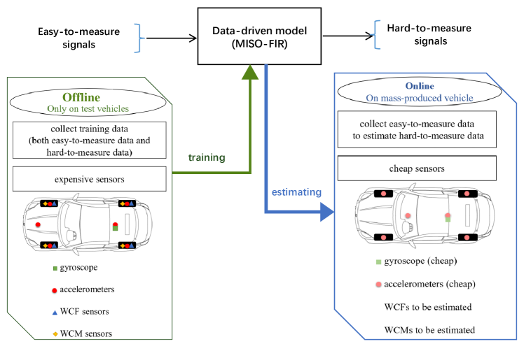
Figure 1: Working principle for online stage and offline stage.

Figure 1 shows the working principle and the background of our work. We use easy-to-measure sensor data (i.e. accelerometers) and hard-to-measure sensor data (i.e. wheel center force data, obtained from WCF sensors) to train the data-driven models offline. For the online stage, we just apply the model by using easy-to-measure sensor data to estimate hard-to-measure sensor data.

Multiple-input single-output finite impulse response (MISO-FIR) models are used. The output of such a model can be expressed as a linear combination of a specific set of input variables [9] as follows,

$$y(t)=\mathbf{a}_{0}^{\mathrm{T}}\mathbf{x}(t)+\ldots+\mathbf{a}_{n}^{\mathrm{T}}\mathbf{x}(t-n)+\bm{\varepsilon}(t),\quad t=n+1,\ldots,M+n,$$ (1)

where $n$ is the order of $\mathbf{x}(t)$, $\mathbf{x}(t)\in\mathbb{R}^{m}$ and ${y}(t)\in\mathbb{R}$ are inputs and output of the MISO-FIR model respectively, $\mathbf{a}_{i}(t)\in\mathbb{R}^{m}$, $i=0,\ldots,n$, are unknown parameters to be estimated, ${\bm{\varepsilon}(t)}$ is the measurement noise of the model, which we assume is independent and identically Gaussian distributed.

We can re-write (1) compactly as

$$\mathbf{Y}=\bm{\Phi}\bm{\theta}+\mathbf{E},$$ (2)

where the model parameter $\bm{\theta}=\left[\mathbf{a}_{0}^{\mathrm{T}}\cdots\mathbf{a}_{n}^{\mathrm{T}}\right]^{\mathrm{T}}$, and

$$\mathbf{Y}=\left[\begin{array}[]{c}y(n+1)\\ \vdots\\ y(M+n)\end{array}\right],\bm{\Phi}=\left[\begin{array}[]{c}\phi^{\mathrm{T}}(n+1)\\ \vdots\\ \phi^{\mathrm{T}}(M+n)\end{array}\right],\mathbf{E}=\left[\begin{array}[]{c}\varepsilon(n+1)\\ \vdots\\ \varepsilon(M+n)\end{array}\right],$$

the regressor $\bm{\phi}(t)=\left[\mathbf{x}^{\mathrm{T}}(t)\cdots\mathbf{x}^{\mathrm{T}}(t-n)\right]^{\mathrm{T}}$.

For each working condition, we construct one data-driven model. However, when there are hundreds of working conditions, we need to build hundreds of data-driven models. This will result in a heavy computational burden on edge devices (in which the soft sensor models have been implemented). Thus, we would like to reduce the computational burden and still keep the estimation accuracy high. In practice, different working conditions may benefit from different sensors. Furthermore, we do not know which working conditions that can be described by the same model. Thus, the difficulties of this work lie in:

• It is an unsupervised learning problem because there are no labels for categories.

• It is a big data problem, subject to dynamics and high-dimension.

• Explainable and generalizable solutions are needed.

3 Methodology

In this section, we first introduce the “Quadratic Parameter Difference Difference Regularization" algorithm and talk about the choice of the hyperparameter for this algorithm. Then, take the sparsity into account, and we propose the “Parameter Difference 2-Norm $\&$ Lasso Regularization" algorithm. Next, we discuss the choice of hyperparameters for the proposed algorithm. Finally, the clustering part is discussed followed by a summary of the algorithm.

3.1 Parameter Difference 2-Norm $\&$ Lasso Regularization

In our case, it is in the order of hundreds. One task is now to eliminate sensors that do not contribute to a model. This corresponds to determining which elements of $\theta_{k}$ are zero. Another task is to determine for which working conditions the same model can be used. As already mentioned, this is important in order to reduce the computational load of the soft-sensor itself. However, another reason is that the model accuracy can be improved if multiple working conditions can be used to estimate the model. Instead of performing the three tasks of model parameter estimation, sensor elimination and model clustering separately, we employ one single criterion where each of these requirements is encoded in a separate term: i) a term measuring the total squared model error, ii) a term measuring the distance between the different models, and iii) a term measuring the importance of each sensor. For the third term, we use the $\ell_{1}$-norm, i.e. lasso, as it is known to lead to sparse solutions [15]. For the second term, we use the Euclidean distance between the parameter vectors of different models. In comparison with group lasso [16], rather than forcing an entire parameter vector to be zero, we are in this way forcing the difference between parameter vectors to be zero, thus achieving that the models are clustered. In summary, we propose the following criterion

$$\mathop{\min}_{\theta_{1}\cdots\theta_{K}}\sum_{k=1}^{K}\|Y_{k}-\Phi_{k}\theta_{k}\|_{2}^{2}+\frac{1}{2}\lambda_{1}\sum_{k,i=1}^{K,K}\|\theta_{k}-\theta_{i}\|_{2}+\lambda_{2}\sum_{k,j=1}^{K,J}\|\theta_{k}^{j}\|_{1},$$ (3)

where, $\lambda_{1}$, and $\lambda_{2}$ are positive constants that are used to control the trade-off among the model fit (the first term), the clustering (the second term), and sparsity (the third term) of the model parameters. $\lambda_{1}$ is the penalty term coefficient of the inter-group, $\lambda_{2}$ is the penalty term coefficient of the intra-group (which shows the sparsity of model parameters within one model). $\theta_{k}$ is the model parameter of working condition $k$. $j=1,\cdots,J$ are the types of different sensors inside one working condition. For example, $\theta_{k}^{j}$ is the parameter of working condition $k$ and sensor channel $j$. Thus, we have $\theta_{k}=[\theta_{k}^{1\rm{T}},\cdots,\theta_{k}^{J\rm{T}}]^{\rm{T}}$. The novelty of this method is that it can not only cluster any two model parameters but can also make a sparsity among the sensor channels within one model. It is of great significance in the real life.

3.2 Choosing the Hyperparameters

Recall that the objective is to be able to eliminate sensors that do not contribute significantly to the estimate of the target signal, and to group together working conditions that can be modeled in the same way. To this end, the parameter $\lambda_{2}$ controls the sparsity and the parameter $\lambda_{1}$ how many different parameter vectors are forced to resemble one another. Picking these parameters too low does not achieve these objectives, while too large values will sacrifice the model fit as given by the first term in (3). It is thus necessary to find a good balance between these conflicting objectives. Starting with $\lambda_{1}$, we have the following result.

Theorem 1.

Let $Y_{k}\in\mathbb{R}^{M_{k}}$, $\Phi_{k}\in\mathbb{R}^{M_{k}\times n_{\theta}}$, $\theta_{k}\in\mathbb{R}^{n_{\theta}},k=1,\cdots,K$, $\lambda_{2}=0$, consider the optimization problem (3). Define

$$\lambda_{1\rm{max}}=\max_{k\in\{1,\cdots,K\}}\left\{\frac{2}{K-1}\|\Phi_{k}^{\rm{T}}[Y_{k}-\Phi_{k}\cdot\theta_{k}]\|_{2}\right\}.$$ (4)

Given that $\lambda_{1}\geq\lambda_{1\rm{max}}$ and $\Phi_{k}^{\rm{T}}\Phi_{k}\succ 0$, $\forall k\in{1,\cdots,K}$, the solution of (3) is given by

$$\theta_{k}=\theta_{\star}=\mathop{\rm{arg}\min}_{\theta}\sum_{k=1}^{K}\|Y_{k}-\Phi_{k}\theta\|_{2}^{2},k=1,\cdots,K.$$ (5)

Theorem 1 gives an upper bound for $\lambda_{1}$ that can be easily computed. In [17] there is a corresponding upper bound for $\lambda_{2}$, given by $\lambda_{2\rm{max}}=\max\left\{2\|\Phi_{k}^{\rm{T}}Y_{k}\|_{1}\right\},k=1,\ldots,K$. For $\lambda_{2}>\lambda_{2\rm{max}}$, it holds that $\theta_{k}^{j}=0$ for all $k,j$.

To find appropriate penalty coefficients, we use grid search. To make the selection of these hyperparameters, we estimate the model parameters $\theta_{k}$ on an estimation dataset, and then pick the $\lambda_{1}$ and $\lambda_{2}$ that minimize (4) on a validation dataset. We use the logaritmically spaced grids $\lambda_{1}=[0.00001\lambda_{1\rm{max}},\cdots,0.1\lambda_{1\rm{max}},\lambda_{1\rm{max}}]$, $\lambda_{2}=[0,10^{-6},10^{-4},10^{-2},1,10^{2}]$ (which are inside the boundary of $\lambda_{2}$).

3.3 Clustering

While the proposed algorithm forces models corresponding to different operating points to become close (due to the term for which $\lambda_{1}$ is a factor), the parameters may not become identical since the same tuning parameter $\lambda_{1}$ is used for all parameter differences. Therefore, we will use a post-processing step where a clustering algorithm is used to merge models. While there is a wide range of clustering algorithms available, we will use K-means in the experimental section. A potential improvement of the algorithm would be to tune the weights for different parameter differences $\|\theta_{k}-\theta_{i}\|_{2}$ individually. However, this would dramatically increase the number of hyperparameters that require tuning.

3.4 Summary

• Step 1: Calculate the boundary of the inter-group penalty term coefficient $\lambda_{1\rm{max}}$ using (5).

• Step 2: Use grid search to choose the two hyperparameters $\lambda_{1}$ and $\lambda_{2}$.

• Step 3: Estimate the model parameter $\theta_{k}$ using hyperparameters obtained from the step before.

• Step 4: Use k-means to cluster different kinds of models.

4 Experiments

4.1 Experimetal Setup

All the experiments are conducted using a 1.60 GHz Intel Core i5-8250U processor. The algorithm implementation is done in Matlab 2021b. The data used in this work is collected from multiple accelerometers and torque sensors installed on a prototype PT-4WD vehicle. Figure 3 shows the vehicle used for field tests, and the red boxes indicate the places where the torque sensors are installed, which can measure the torque in X, Y, and Z directions when driving and braking. Figure 3 shows the 3-axis accelerometers installed on wheels.

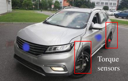
Figure 2: The torque sensors installed on the field test vehicle.

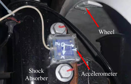
Figure 3: The accelerometers (three-axis) installed on wheels.

The datasets used in this work are named, for example, “BR30-1", where the “BR" refers to the braking working condition, “30" is the speed of the vehicle (i.e., 30km/h), and “1" is the index of the datasets (i.e., the first set under this condition). All datasets used in this work follow this format and each set includes system signals obtained from the multiple sensors during the field tests. In this paper, we use 3 working conditions randomly chosen from the hundreds of available datasets to demonstrate the effectiveness of the proposed algorithm, namely: BR30, BR40, and WBA40, where WBA is the abbreviation of the “Washboard Asynchronous" working condition.

For each working condition, we have hundreds of sensor categories. In this paper, 4 easy-to-measure sensors are chosen as the inputs to estimate the one hard-to-measure sensor. The definitions of the input sensors and output sensor are shown in Table 1. The model order is taken as n=50, which gives 200 parameters to estimate for each working condition as we have 4 inputs. The first 50 parameters are the parameters of the first sensor, whose number is the “throttle pedal (number 57 sensor, see Tab.1)". The 51-100 parameters represent the second sensor, which is the “road surface roughness". Parameters 101-150 and 151-200 are “Right front suspension displacement" and “Left front suspension displacement" respectively.

Table 1: Definitions of the input sensors and output sensor.

	Sensor Number	Category
	57	Throttle pedal
Input	90	Road surface roughness
Sensors	91	Right front suspension displacement
	92	Left front suspension displacement
Output	35	Left front wheel center force in the Z direction.

4.2 Experimental Results

4.2.1 Parameter Comparison

Figure 4 shows the estimated parameter vector for the three different operating conditions when each parameter vector has been estimated separately using least-squares (3). Figure 5 shows the corresponding estimates when the proposed approach has been used in.

Figure 4: Least-squares estimate of $\theta$ for the three used working conditions.

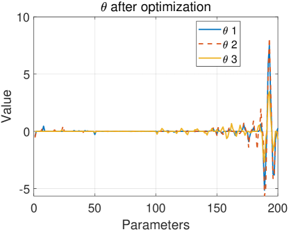
Figure 5: The resulting parameter estimates for the three used working conditions when the proposed algorithm is used.

By comparing the two figures, it can be observed that the parameters of the first sensor have noticeable values when standard least-squares estimation is used. However, they are nearly compressed to zero after applying our proposed algorithm. This indicates that the signal from this sensor contributes little to the estimation of the output sensor signal, and can therefore be considered an “irrelevant sensor". The parameter values of the second sensor are nearly zero both before and after optimization, indicating that this sensor makes a minimal contribution to estimating the output sensor signal, which is also an “irrelevant sensor". The third sensor has small values both before and after optimization, indicating a modest contribution to estimating the target sensor signal. The fourth sensor has large values both before and after optimization, making a significant contribution to estimating the target sensor signal. The penalty coefficients $\lambda_{1}$ and $\lambda_{2}$ are tuned as described in Section II, resulting in the inter-group penalty term coefficient $\lambda_{1}=0.00001\lambda_{1\rm{max}}=0.0369$, and the intra-group penalty term coefficient $\lambda_{2}=1$.

4.2.2 Model Classification

Different kinds of classification algorithms can be used to classify the models. Here, we just choose K-means, which is a fundamental clustering algorithm. We choose the cluster number $K=2$. Table 2 shows the classification results of the three working conditions. It shows that BR30 and BR40 are described by the same model, while WBA40 is classified to require another model.

Table 2: Classification results of the three working conditions.

Working condition	Category
BR30	Category 1
BR40	Category 1
WBA40	Category 2

4.2.3 Model Evaluation

To evaluate the performance of the proposed approach, we use the goodness of FIT [18], defined as

$$FIT=\left(1-\frac{\|Y-\hat{Y}\|_{2}^{2}}{\|Y-\bar{Y}\|_{2}^{2}}\right)\times 100\%,$$ (6)

where $Y$ are measurements collected from the sensors, $\hat{Y}$ is the estimated value obtained from the proposed algorithm, and $\bar{Y}$ is the mean vector of $Y$. The closer the value of FIT to $100\%$, the better the performance is.

To study how well the proposed method is able to classify the different working conditions (cf. Table II), we have estimated one model each, using least-squares, for the three working conditions and then computed the FITs when each of these models is applied to validation data sets coming from all three different working conditions. The results of this can be found in the first three columns of Table III. From the first block rows, it can be seen that working conditions BR30 and BR40 result in models that can be used for both BR30 and BR40, but not for WBA40. The last block row shows that the model estimated using WBA40-1 works well on validation data from the same working condition but not for BR30 and BR40. These results suggest that BR30 and BR40 can be represented with one common model, while a separate model is needed for WBA40. This is consistent with the outcome of the proposed method as indicated in Table 2. Table 4 shows the effectiveness after classification, which verifies our classification results in Table 2.

Table 3: FIT on evaluation data

Dataset for	Dataset for which	FIT using	FIT using
estimated	the FIT	least-square	the proposed
model	is computed	estimate	method
	BR30-2	76.49$\%$	76.44$\%$
BR30-1	BR40-2	75.46$\%$	74.19$\%$
	WBA40-2	-7.53$\%$	44.12$\%$
	BR30-2	74.21$\%$	75.38$\%$
BR40-1	BR40-2	75.65$\%$	75.63$\%$
	WBA40-2	5.80$\%$	46.61$\%$
	BR30-2	44.10$\%$	-6.41$\%$
WBA40-1	BR40-2	46.58$\%$	6.33$\%$
	WBA40-2	73.18$\%$	73.30$\%$

Table 4: FIT on evaluation data after classification

Dataset for	Dataset for which the	FIT using least-square
estimated mode	FIT is computed	estimate
BR30-01 + BR40-01	BR30-02	75.38$\%$
	BR40-02	75.52$\%$
WBA40-01	WBA40-02	73.18$\%$

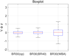
Figure 6: Boxplot for the BR30-2 working condition.

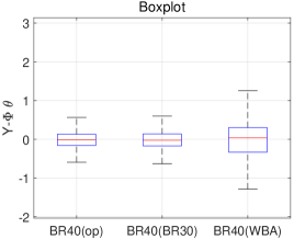
Figure 7: Boxplot for the BR40-2 working condition.

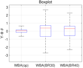
Figure 8: Boxplot for the WBA40-2 working condition.

Figure 9: Comparison between the output signal (see Table 1) for the BR30-2 working condition, and the estimated output using the BR30-1 dataset.

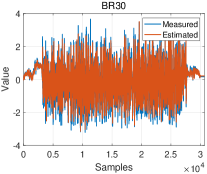
Figure 10: Comparison between the output signal (see Table 1) for the BR30-2 working condition, and the estimated output using the BR40-1 dataset.

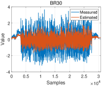
Figure 11: Comparison between the output signal (see Table 1) for the BR30-2 working condition, and the estimated output using the WBA40-1 dataset.

Figure 11,11, and 11 show the boxplot of the cross-evaluation performance of BR30-2, BR40-2, and WBA40-2 working conditions respectively. The content inside the parentheses is the cross-evaluation target, for example, BR30 (BR40) means that use parameters of BR40 to estimate BR30. It can be observed that the performance of the cross-evaluation between BR30 and WBA40, BR40 and WBA40 is not satisfied. Figure 11 shows the cross-evaluation between BR30 and BR40, and Fig.11 shows the cross-evaluation between BR30 and WBA40. It shows that the cross-evaluation effect between BR30 and BR40 is good, while the performance is poor between BR30 and WBA40. This also indicates that our classification results are good.

Alternatively to using the Euclidean norm for terms in the second sum in (4), one can use the squared Euclidean distance. This has been tested with similar results. Results show that $\ell_{2}$-norm with square just accelerates the algorithm within a small range. In this work, we just use the $\ell_{2}$-norm-norm for the inter-group.

5 Conclusion

This article contributes with a lasso-type algorithm based on MISO-FIR and K-means within the soft sensor framework, to classify multiple working conditions with irrelevant sensors into fewer working conditions. Validation with field test datasets from a prototype vehicle shows good performance for the classification. The problem discussed in this paper is very common in practical applications such as the estimation of vehicle dynamics. For future work, we will extend the classification of working conditions to include more scenarios.

References

- [1] E. Risaliti, J. Van Cauteren, T. Tamarozzi, B. Cornelis, and W. Desmet, “Virtual sensing of wheel center forces by means of a linear state estimator,” in International Conference on Noise and Vibration Engineering (ISMA2016), Leuven, Belgium, 2016.
- [2] X. Zhu and W. Li, “Takagi–sugeno fuzzy model based shaft torque estimation for integrated motor–transmission system,” ISA transactions, vol. 93, pp. 14–22, 2019.
- [3] Y. Jiang, S. Yin, J. Dong, and O. Kaynak, “A review on soft sensors for monitoring, control, and optimization of industrial processes,” IEEE Sensors Journal, vol. 21, no. 11, pp. 12 868–12 881, 2020.
- [4] Y. Wang, X. Zheng, L. Wang, G. Lu, Y. Jia, Y. Qiu, and M. Li, “Edge-computing based soft sensors with local finite impulse response models for vehicle wheel center loads estimation under multiple working conditions,” Control Engineering Practice, vol. 133, p. 105447, 2023.
- [5] D. Wang, J. Gong, Q. Kang, D. Fan, and J. Yang, “Soft sensing for gas-condensate field production using parallel-genetic-algorithm-based data reconciliation,” Journal of Computing and Information Science in Engineering, vol. 19, no. 4, p. 044501, 2019.
- [6] X. Fang, X. Li, and L. Xie, “3-d distributed localization with mixed local relative measurements,” IEEE Transactions on Signal Processing, vol. 68, pp. 5869–5881, 2020.
- [7] P. Kadlec, B. Gabrys, and S. Strandt, “Data-driven soft sensors in the process industry,” Computers & chemical engineering, vol. 33, no. 4, pp. 795–814, 2009.
- [8] J. Kang, Z. Shao, X. Chen, X. Gu, and L. Feng, “Fast and reliable computational strategy for developing a rigorous model-driven soft sensor of dynamic molecular weight distribution,” Journal of Process Control, vol. 56, pp. 79–99, 2017.
- [9] L. Ljung, System Identification: Theory for the User, 2nd ed. Englewood Cliffs, NJ: Prentice-Hall, 1999.
- [10] L. Wang, X. Zheng, Y. Wang, Y. Qiu, and M. Li, “A hybrid data-driven soft sensor framework for torque estimation,” IEEE Sensors Journal, 2023.
- [11] X. Zheng, Y. Wang, L. Wang, R. Cai, M. Li, and Y. Qiu, “Data-driven sensor selection for signal estimation of vertical wheel forces in vehicles,” Journal of Computing and Information Science in Engineering, vol. 23, no. 3, p. 031010, 2023.
- [12] N. Rao, R. Nowak, C. Cox, and T. Rogers, “Classification with the sparse group lasso,” IEEE Transactions on Signal Processing, vol. 64, no. 2, pp. 448–463, 2015.
- [13] D. Ghosh and A. M. Chinnaiyan, “Classification and selection of biomarkers in genomic data using lasso,” Journal of Biomedicine and Biotechnology, vol. 2005, no. 2, p. 147, 2005.
- [14] Y. Huo, L. Xin, C. Kang, M. Wang, Q. Ma, and B. Yu, “Sgl-svm: a novel method for tumor classification via support vector machine with sparse group lasso,” Journal of Theoretical Biology, vol. 486, p. 110098, 2020.
- [15] R. Tibshirani, “Regression shrinkage and selection via the LASSO,” Journal of the Royal Statistical Society. Series B, vol. 58, no. 1, pp. 267–288, 1996.
- [16] M. Yuan and Y. Lin, “Model selection and estimation in regression with grouped variables,” Journal of the Royal Statistical Society. Series B, vol. 68, no. 1, pp. 49–67, 2006.
- [17] L. Yuan, J. Liu, and J. Ye, “Efficient methods for overlapping group lasso,” Advances in neural information processing systems, vol. 24, 2011.
- [18] G. H. Golub and C. F. Van Loan, Matrix computations. JHU press, 2013.