Light-induced Hall currents in altermagnets

Abstract

Berry curvature, a momentum space property, can manifest itself in current responses. The well-known anomalous Hall effect in time-reversal-breaking systems arises from a Berry curvature monopole. In time-reversal-invariant materials, a second-order Hall conductivity emerges from a Berry curvature dipole. Recently, it has been shown that a Berry curvature quadrupole induces a third-order ac Hall response in systems that break time reversal ($K$) and a fourfold rotational ($C_{4}$) symmetry, while remaining invariant under the combination of the two ($C_{4}K$). In this letter, we demonstrate that incident light can induce a $\rm dc$ Hall current in such systems, driven by the Berry curvature quadrupole. We consider a combination of a static $\rm dc$ electric field and an ac light-induced electric field. We calculate the current perpendicular to both the static electric field and the fourfold axis. Remarkably, the induced current is generically spin-polarized. A net charge current appears for light that is linearly or elliptically polarized, but not for circular polarization. In contrast, the spin current remains unchanged when the polarization of light is varied. This allows for rich possibilities such as generating a spin current by shining circularly polarized light on an altermagnetic material. We demonstrate this physics using a two-dimensional toy model for altermagnets.

Introduction.—  Current responses provide an experimentally accessible window into the Berry curvature properties of electronic bands [1, 2]. In particular, the quantum Hall effect and the anomalous Hall effect serve as powerful tools across material families [3, 4, 5, 6, 7, 8, 9, 10]. The latter has been conceptualized as an expansion in moments of the Berry curvature distribution over the Brillouin zone – the $n^{\mathrm{th}}$ moment yields a response at the $(n+1)^{\mathrm{th}}$ order in the applied electric field [11]. A monopole component ($n=0$), which can only exist when time reversal (TR) symmetry is broken, yields a linear response [2, 6, 12]. A dipole moment ($n=1$) gives rise to a non-linear second-order response [13], which has been measured in ${\rm WTe}_{2}$ [14, 15, 16] and other materials [17, 18, 19, 20]. Recent studies have probed the quadrupole moment ($n=2$) and its third-order response [21, 22, 23, 24, 25, 26, 27]. This has been measured in FeSn, as a transverse voltage generated at three times the frequency of the applied field [28]. In this letter, we show that the same physics can yield a $\rm dc$ response when a $\rm dc$ applied field is combined with light.

The Berry curvature and its moments are strongly constrained by the symmetries of the material. We focus on materials that break time reversal (TR) symmetry $K$ and a fourfold rotational symmetry $C_{4}$, while preserving their combination $C_{4}K$. In this case, the Berry curvature monopole and dipole moments must vanish, so that the leading contribution comes from a quadrupole moment. The $C_{4}K$ symmetry is realized in altermagnets [29, 30, 31] as well as in magnetically ordered materials belonging to certain magnetic point groups [26]. Any material with this symmetry will generically have spin-polarized bands. We demonstrate that the Hall response will also be generically spin-polarized. Intriguingly, the very same symmetry requirements are also invoked in chiral higher order topological crystalline insulators [32]. Here, we restrict our attention to metallic systems where the Hall response appears as a Fermi-surface property [33, 34].

Our results provide a counterpoint to the photovoltaic Hall effect, first proposed in graphene [35, 36]. This effect uses a combination of a $\rm dc$ electric field and circularly polarized light to induce a transverse $\rm dc$ current. Circular polarization can be viewed as a TR symmetry-breaking field, akin to the magnetic field in the usual Hall effect. In contrast, our results pertain to materials with inherent time-reversal breaking such as altermagnets. A Hall current is produced by linearly or elliptically polarized light, but not when the polarization is circular. Moreover, this Hall current carries nonzero spin polarization.

Framework.—  We consider a metal with a single band crossing the Fermi level. We use semiclassical wavepacket dynamics [2] to describe transport, denoting wavepacket position as $\bm{r}$ and momentum as $\bm{k}$. Following the well-known semiclassical prescription, its velocity is given by $\dot{\bm{r}}=\bm{v}-\bm{k}\times\bm{\Omega}$, where $\bm{v}$ is the group velocity (we use units in which $\hbar=1$). An anomalous velocity contribution arises from the Berry curvature ${\bm{\Omega}}$ [12, 2, 6]. Neglecting external magnetic fields, momentum evolves according to $\dot{\bm{k}}=-e[\bm{E}+\bm{E}_{\rm ac}(t)]$, where the total applied electric field is a combination of a static field $\bm{E}$ and a light-induced field $\bm{E}_{\rm ac}$, as shown in Fig. 1. The latter is given by $\bm{E}_{\rm ac}(t)={\rm Re}(\bm{\mathcal{E}}e^{-i\omega t})$, where $\bm{\mathcal{E}}$ is a complex vector amplitude.

Following the Boltzmann transport paradigm, we define a distribution function $f(\bm{k})$, which satisfies the kinetic equation

$$\frac{\partial f}{\partial t}+\dot{\bm{k}}\,\cdot\frac{\partial f}{\partial\bm{k}}=-\frac{f-f_{0}}{\tau},$$ (1)

where $f_{0}$ is the equilibrium Fermi-Dirac distribution function. The relaxation time $\tau$ is assumed to be a constant for simplicity. Treating the applied electric fields as perturbations, we expand the solution of Eq. (1) in powers of the fields up to third order: $f=f_{0}+f_{1}+f_{2}+f_{3}$. We further divide the distribution into static and time-dependent parts. Keeping only the leading harmonic, we have

$$f_{a}=f^{(0)}_{a}+f_{a}^{(\omega)}e^{-i\omega t}+f_{a}^{(\omega),*}e^{i\omega t}\quad(a=1,2,3).$$ (2)

At first order, $f^{(0)}_{1}\propto E$ and $f_{1}^{(\omega)}\propto\mathcal{E}$. Second-order terms can be written as $f^{(0)}_{2}\propto\mathcal{E}\mathcal{E}^{*}$ and $f_{2}^{(\omega)}\propto E\mathcal{E}$. At third order, we have $f^{(0)}_{3}\propto E\mathcal{E}\mathcal{E}^{*}$ and $f_{3}^{(\omega)}\propto\mathcal{E}\mathcal{E}\mathcal{E}^{*}$. Other contributions, such as $f^{(0)}_{2}\propto EE$, do not affect the Hall currents discussed below. Details of the calculations are given in the Supplemental Material [37].

The electric charge ($c$) current density is given by ${\bm{j}}_{c}=-e\int_{\bm{k}}{\dot{\bm{r}}}\,f(\bm{k})$. Here and below we assume a two-dimensional (2D) system, so that $\int_{\bm{k}}\equiv\int_{\bm{k}}d^{2}k/(2\pi)^{2}$. Focusing on the dc current, we have

$$j_{c,i}= -e\int_{\bm{k}}\sum_{a=1}^{3}v_{i}f_{a}^{(0)}+e^{2}\int_{\bm{k}}\sum_{a=1}^{3}\Omega_{ij}E_{j}f_{a}^{(0)}$$

$$+e^{2}\int_{\bm{k}}\sum_{a=1}^{3}\Omega_{ij}[{\mathcal{E}}_{j}f_{a}^{(\omega),*}+c.c.],$$ (3)

where $i,j=x,y$. In our geometry, the only nonzero component of the Berry curvature is $\Omega(\bm{k})\equiv\Omega_{xy}(\bm{k})$.

We consider the possibility that this current may carry spin polarization. In materials such as altermagnets, Bloch states may have unequal weights in the two spin components [29, 38]. To incorporate this effect, we introduce a spin-polarization function, $s(\bm{k})$, that represents the expectation value of the $z$ component of spin in the Bloch state at momentum $\bm{k}$. Taking our 2D material to lie in the $xy$ plane, it is natural to focus on the spin polarization along $z$. Due to the $C_{4}K$ symmetry, $s(\bm{k})$ must switch sign under a four-fold rotation. The spin-polarized ($s$) component of charge current is given by $\bm{j}_{s}=-e\int_{\bm{k}}{\dot{\bm{r}}}s(\bm{k})f(\bm{k})$. Henceforth, we refer to this simply as “spin current”. It can be expressed in terms of the Fermi-Dirac distribution as in Eq. (3), by simply including a factor of $s(\bm{k})$ in the integrands.

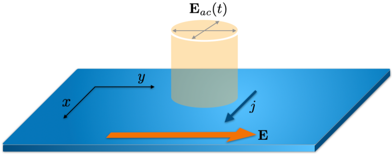
Figure 1: Proposed configuration for the light-induced Hall effect. The sample is assumed to be in the $xy$ plane with a fourfold axis along $z$. A static electric field is imposed along $y$. Light, linear or elliptically polarized, impinges from the $z$ axis. The dc current is measured along $x$.

Symmetry considerations.—  We wish to derive an expression for the Hall current perpendicular to the applied dc field in a 2D material which breaks $C_{4}$ and $K$, but preserves $C_{4}K$. Note that we will also have a $C_{2}$ symmetry, by applying $C_{4}K$ twice. We consider the geometry shown in Fig. 1 and calculate the dc Hall current to third order in applied electric fields. Assuming $\omega\tau$ is small, we obtain

$$j_{c,x}= j^{Q}_{c,x}+j^{D}_{c,x},$$ (4)

where

$$j^{Q}_{c,x}=e^{4}\tau^{2}\Big{(}\int_{\bm{k}}f_{0}~{}\partial_{i}\partial_{j}\Omega\Big{)}E_{y}\mathcal{E}_{i}\mathcal{E}^{*}_{j}$$ (5)

represents the contribution from the Berry curvature quadrupole, defined as $\mathcal{Q}^{c}_{ij}=\int_{\bm{k}}f_{0}\partial_{i}\partial_{j}\Omega$, a Fermi-surface property [33, 34]. The second term in Eq. (4),

$$j^{D}_{c,x}=-e^{4}\tau^{3}\Big{(}\int_{\bm{k}}v_{x}\partial_{i}\partial_{j}\partial_{y}f_{0}\Big{)}E_{y}\mathcal{E}_{i}\mathcal{E}^{*}_{j},$$ (6)

is a Drude-like contribution.

Expressions for the current responses crucially depend on the symmetries of the system. In particular, a Berry monopole contribution is ruled out by the $C_{4}K$ symmetry, whereas the linear Drude and Berry dipole contributions vanish due to the $C_{2}$ symmetry [26]. Therefore, the leading contributions are given by Eqs. (5) and (6). Any further contribution is either at higher order in electric fields or is scaled down by factors of $\omega\tau$.

The light-induced Hall current generically carries spin. As with the charge Hall current, the spin Hall current contains two contributions,

$$j_{s,x}=j^{Q}_{s,x}+j^{D}_{s,x},$$ (7)

where $j^{Q}_{s,x}$ and $j^{D}_{s,x}$ are the Berry-curvature-driven and Drude-like contributions respectively. These contributions are generically nonzero.

Below, we find expressions for the current contributions using only the $C_{4}K$ symmetry. Subsequently, as an explicit demonstration, we evaluate each contribution in a specific model.

Role of polarization—We assume normal incidence of light on the sample with a spot size much larger than the electronic mean free path. In the paraxial approximation [39], the electric field is spatially uniform. Allowing for an arbitrary polarization, the electric field of light of amplitude ${\mathcal{E}}_{\rm ac}$ is described by

$${\mathcal{E}}_{x}={\mathcal{E}}_{\rm ac}\cos\theta,\quad{\mathcal{E}}_{y}={\mathcal{E}}_{\rm ac}e^{i\phi}\sin\theta.$$ (8)

Linear polarization corresponds to $\phi=0$ or $\pi$. Linear polarization along $x$ ($y$) corresponds to $\theta=0$ or $\pi$ ($\pi/2$ or $3\pi/2$) with an arbitrary value of $\phi$. When $|{\mathcal{E}}_{x}|=|{\mathcal{E}}_{y}|$ and $\phi=\pm\pi/2$, the light is circularly polarized. For generic values of $\theta$ and $\phi$, we have elliptical polarization.

With the ac electric field given by Eq. (8), we now calculate each contribution to the current using the $C_{4}K$ symmetry. The Berry quadrupole contribution to the charge Hall current takes the form,

$$j^{Q}_{c,x}=2e^{4}\tau^{2}E_{y}\mathcal{E}_{\rm ac}^{2}\left(\mathcal{Q}^{c}_{xx}\cos 2\theta+\mathcal{Q}^{c}_{xy}\sin 2\theta\cos\phi\right).$$ (9)

Here, $\mathcal{Q}_{ij}^{c}$ is the same as the Berry quadrupole density defined earlier. The Berry quadrupole contribution to the spin Hall current is given by

$$j^{Q}_{s,x}=2e^{4}\tau^{2}E_{y}\mathcal{E}_{\rm ac}^{2}\mathcal{Q}^{s}_{xx},$$ (10)

where we have defined the spin-polarized Berry quadrupole density as $\mathcal{Q}_{ij}^{s}=\int_{\bm{k}}\,s(\bm{k})\,\Omega\partial_{i}\partial_{j}f_{0}$. For the charge current arising from third-order Drude contributions, we obtain

$$j_{x,c}^{D}=-4e^{4}\tau^{3}E_{y}\mathcal{E}_{\rm ac}^{2}\left[\mathcal{M}^{c}_{xxy}\cos 2\theta+\mathcal{M}^{c}_{xyy}\sin 2\theta\cos\phi\right],$$ (11)

where $\mathcal{M}^{c}_{ijk}=\int_{\bm{k}}v_{x}\partial_{i}\partial_{j}\partial_{k}f_{0}$. The Drude spin current is given by

$$j_{x,s}^{D}=-4e^{4}\tau^{3}E_{y}\mathcal{E}_{\rm ac}^{2}\mathcal{M}^{s}_{xxy},$$ (12)

where $\mathcal{M}^{s}_{ijk}=\int_{\bm{k}}v_{x}s(\bm{k})\partial_{i}\partial_{j}\partial_{k}f_{0}$. Expressions (9), (10), (11) and (12) have been derived using the constraints placed by the $C_{4}K$ symmetry on the response integrals. This symmetry ensures that $\mathcal{Q}_{xx}^{c}=-\mathcal{Q}_{yy}^{c}$, $\mathcal{Q}_{xx}^{s}=\mathcal{Q}_{yy}^{s}$, $Q_{xy}^{s}=0$, $\mathcal{M}^{c}_{xxy}=-\mathcal{M}^{c}_{yyy}$, $\mathcal{M}^{s}_{xxy}=\mathcal{M}^{s}_{yyy}$, and finally $\mathcal{M}^{s}_{xyy}=0$ (Sec. S4 B in Supplemental Material [37]).

Remarkably, as seen from Eqs. (9) and (11), both contributions to charge current vanish for circular polarization (e.g., when $\theta=\pi/4$ and $\phi=\pi/2$). The spin current contributions in Eqs. (10) and (12) are independent of $\theta$ and $\phi$. They do not change as the polarization of light is varied.

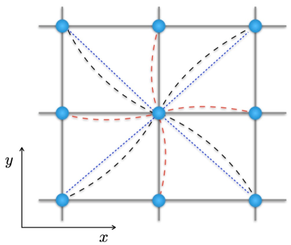
Figure 2: Proposed tight-binding model for a generic $C_{4}K$ material. We have standard hopping processes between nearest neighbours. Along diagonals we have Rashba-like hopping shown as blue dotted lines. Altermagnetic order is captured in two spin-dependent hopping processes: $J_{1}$ between nearest neighbours (red dashed lines) and $J_{2}$ between next nearest neighbours (black dashed lines).

Model and Hamiltonian; $C_{4}K$ symmetry.—  As a concrete demonstration, we build a minimal model with the required symmetries. We begin with a long-wavelength description, followed by a tight-binding model. We consider a 2D system with two bands arising from electron spin. At momenta that are invariant under $C_{4}K$, the two bands must necessarily be degenerate, giving rise to Dirac points.

In the vicinity of each Dirac point, we may write the two-level Hamiltonian as $\hat{H}(\bm{k})=d_{0}({\bm{k}})\hat{\sigma}_{0}+{\bm{d}}(\bm{k})\cdot\hat{\bm{\sigma}}$, where $\hat{\bm{\sigma}}$ is a vector of the Pauli matrices that act on the spin degree of freedom, $\bm{k}$ is measured from the Dirac point, and the coefficients $d_{i}(\bm{k})$ are real functions of $\bm{k}$. With the symmetry group generated by the antiunitary operation $C_{4}K$, at small $\bm{k}$ we have [37]

$$d_{0}(\bm{k}) = a_{0}+a_{1}(k^{2}_{x}+k^{2}_{y}),$$

$$d_{1}(\bm{k}) = b_{1}k_{x}+b_{2}k_{y},$$

$$d_{2}(\bm{k}) = -b_{2}k_{x}+b_{1}k_{y},$$

$$d_{3}(\bm{k}) = m_{1}(k_{x}^{2}-k_{y}^{2})+2m_{2}k_{x}k_{y}.$$ (13)

We have used the lowest-order polynomial expressions for the components of $\bm{d}$. Similar expressions have previously been used as toy models for altermagnets [40]. The Berry curvature can be immediately computed using $\Omega=\epsilon^{ijk}d_{i}\left(\partial_{k_{x}}d_{j}\partial_{k_{y}}d_{k}\right)/{2|\bm{d}|^{3}}$, where $|\bm{d}|=\sqrt{d_{1}^{2}+d_{2}^{2}+d_{3}^{2}}$. This results in a quadrupole-like distribution of $\Omega$ around $\bm{k}=0$ [37]. In the neighbourhood of each Dirac point, we will have a long-wavelength Hamiltonian of the form given in Eq. (13).

To better understand the origin of various terms in the Hamiltonian, we construct a tight-binding model that reproduces Eq. (13). We start with a 2D square lattice as shown in Fig. 2, with the lattice constant set to unity. We expect to find Dirac points at two $C_{4}K$-invariant momenta: $\bm{k}=(0,0)$ and $(\pi,\pi)$, corresponding to $\Gamma$ and $M$ points in the Brillouin zone respectively. Apart from the usual hopping processes, we have spin-dependent hopping between nearest neighbours, which could arise from the Rashba spin-orbit coupling. We introduce the “altermagnetic order parameters” $J_{1}$ and $J_{2}$, which encode preferential hopping of each spin along nearest and next-nearest neighbour bonds. Crucially, the $J_{1}$ and $J_{2}$ processes break $C_{4}$ and $K$, but preserve $C_{4}K$. We arrive at the following Hamiltonian in momentum space:

$$\hat{H}(\bm{k})= -t\big{(}\cos k_{x}+\cos k_{y}\big{)}\hat{\sigma}_{0}$$

$$+\frac{\lambda}{2}\left[\sin\left(k_{x}+k_{y}\right)\hat{\sigma}_{x}+\sin\left(k_{y}-k_{x}\right)\hat{\sigma}_{y}\right]$$

$$+\left[J_{1}(\cos k_{x}-\cos k_{y})+J_{2}\sin k_{x}\sin k_{y}\right]\hat{\sigma}_{z},$$ (14)

where $t$ is the usual hopping parameter and $\lambda$ corresponds to the Rashba spin-orbit coupling.

\begin{overpic}[width=210.30595pt]{t=0.02bandstructureplotJ1J2.png} \put(0.0,100.0){\rm{(a)}} \end{overpic}

\begin{overpic}[width=214.63977pt]{t=0.02mu=0.15fermicircleplot.png} \put(2.0,100.0){\rm{(b)}} \end{overpic}

Figure 3: (a) Band structure and (b) Fermi pockets for $\lambda=0.4$, $\mu=-0.15$, $J_{1}=J_{2}=1$, and $t=0.02$ in arbitrary units of energy.

The resulting band structure is plotted in Fig. 3, for a certain choice of model parameters. Changing the chemical potential affects the shape of the Fermi pockets (Supplemental Material, Figs. S1 and S2 [37]). To proceed analytically, we examine the behavior of the system near the Dirac nodes. Near the $\Gamma$ point, we recover the long-wavelength form of Eq. (13) with $a_{0}=-2t$, $a_{1}=t/2$, $b_{1}=b_{2}=\lambda/2$, $m_{1}=-J_{1}/2$, $m_{2}=J_{2}/2$. Near the $M$ point, we recover the same form, but with $a_{0}=2t$, $a_{1}=t/2$, $b_{1}=b_{2}=\lambda/2$, $m_{1}=J_{1}/2$, and $m_{2}=J_{2}/2$.

At each Dirac node, we have an upper band and a lower band. Their Berry curvatures are given by

$$\Omega^{\eta}_{\pm}=\pm\eta\frac{[J_{1}(k_{x}^{2}-k_{y}^{2})-2\eta J_{2}k_{x}k_{y}]\lambda^{2}}{\left([J_{1}(k_{x}^{2}-k_{y}^{2})-2\eta J_{2}k_{x}k_{y}]^{2}+2\lambda^{2}k^{2}\right)^{3/2}},$$ (15)

where $\eta=+1$ around $\Gamma$ and $-1$ around $M$. The upper (lower) sign applies for the upper (lower) band. Using these expressions, we may evaluate the quadrupole densities, $\mathcal{Q}_{ij}^{c,s}$ , which appear in the charge and spin Hall currents, see Eqs. (9) and (10). Notably, the $J_{1}$ and $J_{2}$ order parameters produce distinct quadrupole patterns. The former can be viewed as creating a $d_{x^{2}-y^{2}}$-wave altermagnet, whereas the latter yields a $d_{xy}$-wave altermagnet (Fig. S3 in the Supplemental Material [37]).

On examining the Bloch states of each band, we find them to be generically spin-polarized. The entries in each eigenspinor have unequal amplitudes. This allows us to define the spin-polarization function

$$s^{\eta}_{\pm}(\bm{k})=\mp\eta\frac{J_{1}(k^{2}_{x}-k^{2}_{y})-2\eta J_{2}k_{x}k_{y}}{\sqrt{[J_{1}(k_{x}^{2}-k_{y}^{2})-2\eta J_{2}k_{x}k_{y}]^{2}+2\lambda^{2}k^{2}}},$$ (16)

which enters the spin Hall current in Eqs. (7), (10) and (12).

Light-induced Hall currents.—  As an explicit demonstration, we calculate light-induced Hall current with the following simplifying assumptions. The Fermi energy is taken to be close to both Dirac points, resulting in two small Fermi pockets. We further assume weak altermagnetic order with $J_{1},J_{2}\ll\lambda$. This results in nearly circular Fermi surfaces (Supplemental Material [37]). Below, we calculate current contributions to leading order in $J_{1,2}/\lambda$. For concreteness, we suppose that the Fermi energy crosses the lower band at each pocket. Neglecting inter-pocket scattering, the charge and spin currents acquire contributions from each pocket separately.

The charge current induced by the Berry curvature quadrupole is obtained from Eq. (9), including contributions from both Fermi pockets:

$$j^{Q}_{c,x}= \frac{e^{4}\tau^{2}}{16\pi}E_{y}{\mathcal{E}}_{\rm ac}^{2}\bigg{[}J_{1}\left(\frac{1}{|\epsilon_{\Gamma}-\mu|}-\frac{1}{|\epsilon_{M}-\mu|}\right)\cos 2\theta$$

$$+J_{2}\left(\frac{1}{|\epsilon_{\Gamma}-\mu|}-\frac{1}{|\epsilon_{M}-\mu|}\right)\sin 2\theta\cos\phi\bigg{]},$$ (17)

where $\epsilon_{\Gamma}$ and $\epsilon_{M}$ are the energies of the degenerate bands at the $\Gamma$ and $M$ points, respectively. $\mu$ is the chemical potential. The quadrupole-induced spin current of Eq. (10) takes the form

$$j^{Q}_{s,x}=\frac{e^{4}\tau^{2}}{64\pi}\frac{(J_{1}^{2}+J_{2}^{2})^{2}}{\lambda^{4}}E_{y}{\mathcal{E}}_{\rm ac}^{2}\bigg{[}\frac{|\epsilon_{\Gamma}-\mu|^{2}}{\lambda^{2}}+\frac{|\epsilon_{M}-\mu|^{2}}{\lambda^{2}}\bigg{]}.$$ (18)

These expressions show that the quadrupole-induced Hall currents arise from the altermagnetic order parameters, $J_{1}$ and $J_{2}$. If these order parameters were to vanish, so would the Berry-curvature quadrupole and its contribution to the dc Hall current.

We next calculate the Drude current by including contributions from the two Fermi pockets. The Drude charge current of Eq. (11) comes out to be

$$j^{D}_{c,x}= \frac{e^{4}\tau^{3}\lambda^{2}}{8\pi}E_{y}{\mathcal{E}}_{\rm ac}^{2}\bigg{[}\left(\frac{1}{|\epsilon_{\Gamma}-\mu|}+\frac{1}{|\epsilon_{M}-\mu|}\right)\sin 2\theta\cos\phi$$

$$+\frac{3}{2}\frac{J_{1}J_{2}}{\lambda^{4}}\big{(}|\epsilon_{\Gamma}-\mu|+|\epsilon_{M}-\mu|\big{)}\cos 2\theta\bigg{]},$$ (19)

whereas the Drude spin current of Eq. (12) yields

$$j^{D}_{s,x}=\frac{e^{4}\tau^{3}J_{2}}{2\pi}E_{y}{\mathcal{E}}_{\rm ac}^{2}.$$ (20)

Conclusion.— In Eqs. (17)-(20), we present explicit analytical results for a specific altermagnetic model. We emphasize two features that are model-independent: (i) the charge Hall current vanishes when light is circularly polarized, and (ii) the spin current does not vary with polarization. These features arise solely from the $C_{4}K$ symmetry.

Our results can be readily tested by shining light on altermagnetic materials such as $\rm{RuO_{2}}$, $\rm{MnO_{2}}$ and $\rm{MnF_{2}}$ [30, 29]. Light-induced currents complement various other transport properties known in altermagnets [41, 42, 43, 44, 45]. Light can also provide a technological advantage, as a switch to generate currents on demand.

Acknowledgments.—  We thank R. Shankar, A. Soori, S. A. Jafari, R. Ghadimi, and K. Farain for helpful discussions. This work was supported by the Natural Sciences and Engineering Research Council of Canada through Discovery Grants 2022-05240 (RG) and 2021-03705 (KS).

I Semiclassical equations of motion

In the semiclassical description of transport, the electric current density can be expressed in terms of the distribution function $f({\bm{k}})$ as

$$j_{i}=-e\int_{\bm{k}}{\dot{r}}_{i}f(\bm{k}),$$ (S21)

where $\int_{\bm{k}}\equiv\int d^{d}{\bm{k}}/(2\pi)^{d}$ in $d$ dimensions and ${\dot{\bm{r}}}$ is the velocity of a wavepacket. The velocity obeys the semiclassical equations of motion, modified by the Berry curvature [46, 6, 12, 47],

$$\dot{r}_{i}=v_{i}+\Omega_{ij}\dot{k}_{j},$$ (S22)

and

$$\dot{k}_{i}=-e[E_{i}+E_{{\rm ac},i}(t)].$$ (S23)

Here, $\Omega_{ij}$ is the Berry curvature and $\bm{v}$ is the group velocity. The total applied electric field is a combination of a static field $\bm{E}$ and a light-induced field $\bm{E}_{\rm ac}$. The latter is given by $\bm{E}_{\rm ac}(t)={\rm Re}(\bm{\mathcal{E}}e^{-i\omega t})$, where $\bm{\mathcal{E}}$ is a complex vector. In the relaxation time approximation, the electron distribution function follows the Boltzmann equation,

$$\frac{\partial f}{\partial t}+\dot{k}_{i}\frac{\partial f}{\partial k_{i}}=-\frac{f-f_{0}}{\tau},$$ (S24)

where $f_{0}$ represents the equilibrium Fermi distribution function and $\tau$ denotes the relaxation time, assumed to be a constant for simplicity. By inserting Eq. (S23) we have

$$\frac{\partial f}{\partial t}-e[E_{i}+E_{{\rm ac},i}(t)]\frac{\partial f}{\partial k_{i}}=-\frac{f-f_{0}}{\tau}.$$ (S25)

Treating the applied electric fields as perturbations, we expand the solution of Eq. (S25) in powers of the fields up to third order:

$$f=f_{0}+f_{1}+f_{2}+f_{3}.$$ (S26)

We further divide the distribution into static and time-dependent parts. Keeping only the leading harmonic, we have

$$f_{a}=f^{(0)}_{a}+f_{a}^{(\omega)}e^{-i\omega t}+f_{a}^{(\omega),*}e^{i\omega t}\quad(a=1,2,3),$$ (S27)

where $a$ represents the order of the expansion in electric fields. We substitute the expansion of Eq. (S27) into Eq. (S25) and solve for each component of $f$ using an order-by-order approach, proceeding sequentially from lower to higher orders. At first order, $f^{(0)}_{1}\propto E$ and $f_{1}^{(\omega)}\propto\mathcal{E}$. Second-order terms can be written as $f^{(0)}_{2}\propto\mathcal{E}\mathcal{E}^{*}$ and $f_{2}^{(\omega)}\propto E\mathcal{E}$. At third order, we have $f^{(0)}_{3}\propto E\mathcal{E}\mathcal{E}^{*}$ and $f_{3}^{(\omega)}\propto\mathcal{E}\mathcal{E}\mathcal{E}^{*}$. We neglect certain contributions, such as $f^{(0)}_{2}\propto EE$, that do not impact the Hall current. We find

$$f_{1}^{(0)}=e\tau E_{i}\partial_{i}f_{0},$$

$$f_{1}^{(\omega)}=\frac{e\tau\mathcal{E}_{i}}{1-i\omega\tau}\partial_{i}f_{0},$$

$$f^{(0)}_{2}=e^{2}\tau^{2}\left(\frac{\mathcal{E}^{*}_{i}\mathcal{E}_{j}}{1-i\omega\tau}+\frac{\mathcal{E}_{i}\mathcal{E}^{*}_{j}}{1+i\omega\tau}\right)\partial_{i}\partial_{j}f_{0},$$

$$f_{2}^{(\omega)}=e^{2}\tau^{2}\left(\frac{E_{i}\mathcal{E}_{j}}{(1-i\omega\tau)^{2}}+\frac{E_{j}\mathcal{E}_{i}}{1-i\omega\tau}\right)\partial_{i}\partial_{j}f_{0},$$

$$f_{3}^{(0)}=e^{3}\tau^{3}\left(\frac{\mathcal{E}_{i}^{*}\mathcal{E}_{j}E_{k}}{(1-i\omega\tau)^{2}}+\frac{\mathcal{E}_{i}^{*}\mathcal{E}_{k}E_{j}}{1-i\omega\tau}+\frac{\mathcal{E}_{i}\mathcal{E}_{j}^{*}E_{k}}{(1+i\omega\tau)^{2}}+\frac{\mathcal{E}_{i}\mathcal{E}_{k}^{*}E_{j}}{1+i\omega\tau}\right)\partial_{i}\partial_{j}\partial_{k}f_{0},$$

$$f_{3}^{(\omega)}=e^{3}\tau^{3}\left(\frac{\mathcal{E}_{i}\mathcal{E}^{*}_{j}\mathcal{E}_{k}}{(1-i\omega\tau)(1-i\omega\tau)}+\frac{\mathcal{E}_{i}\mathcal{E}_{j}\mathcal{E}^{*}_{k}}{(1+i\omega\tau)(1-i\omega\tau)}\right)\partial_{i}\partial_{j}\partial_{k}f_{0}.$$ (S28)

II dc current

The dc current charge density is given by the expression

$$j^{(0)}_{i}=-e\int_{\bm{k}}\sum_{n}v_{i}f_{n}^{(0)}+e^{2}E_{j}\int_{\bm{k}}\sum_{n}\Omega_{ij}f_{n}^{(0)}+e^{2}\int_{\bm{k}}\sum_{n}\Omega_{ij}[\mathcal{E}_{j}f_{n}^{(\omega),*}+c.c.].$$ (S29)

Substituting the explicit solutions (S28) into Eq. (S29), we arrive at

$$j^{(0)}_{i} =-e\int_{\bm{k}}v_{i}f_{0}+e^{2}E_{j}\int_{\bm{k}}\Omega_{ij}f_{0}-e^{2}\tau E_{j}\int_{\bm{k}}v_{i}\partial_{j}f_{0}+e^{3}\tau E_{j}E_{k}\int_{\bm{k}}\Omega_{ij}\partial_{k}f_{0}$$

$$+\biggl{\{}\frac{e^{3}\tau}{1+i\omega\tau}\mathcal{E}_{j}\mathcal{E}_{k}^{*}\left[\int_{\bm{k}}\Omega_{ij}\partial_{k}f_{0}-e\tau\int_{\bm{k}}v_{i}\partial_{j}\partial_{k}f_{0}\right]+c.c.\biggr{\}}$$

$$+\biggl{\{}\frac{e^{4}\tau^{2}}{1+i\omega\tau}E_{j}\mathcal{E}_{k}\mathcal{E}^{*}_{m}\left[\int_{\bm{k}}\Omega_{ij}\partial_{m}\partial_{k}f_{0}~{}-\frac{\tau}{1+i\omega\tau}\int_{\bm{k}}v_{i}\partial_{k}\partial_{m}\partial_{j}f_{0}-\tau\int_{\bm{k}}v_{i}\partial_{k}\partial_{j}\partial_{m}f_{0}\right]+c.c.\biggr{\}}.$$ (S30)

The term $D_{k;ij}=\int_{\bm{k}}f_{0}~{}(\partial_{k}\Omega_{ij})=-\int_{\bm{k}}\Omega_{ij}\partial_{k}f_{0}$ is referred to as the Berry curvature dipole [13], while

$$Q_{km;ij}=\int_{\bm{k}}f_{0}(\partial_{k}\partial_{m}\Omega_{ij})=\int_{\bm{k}}\Omega_{ij}\partial_{k}\partial_{m}f_{0}$$ (S31)

is called the Berry curvature quadrupole [21, 26]. As we work in two dimensions, only one component of the Berry curvature, $\Omega_{xy}$, is non-zero. As discussed in the main text, the symmetries in the problem impose some constraints on the integrals in Eq. (S30). With the $C_{4}K$ symmetry, the Hall current (perpendicular to the static field) will only receive contributions at third order in the electric field. We focus on these terms in the following sections.

II.1 Charge current

We now present explicit expressions for the current contributions that arise from various combinations of electric fields. We assume that the static field is along $y$, i.e. ${\bm{E}}=E_{y}\hat{\bm{y}}$, whereas the ac field can have both $x$ and $y$ components. Below, we list the third-order terms proportional to $E_{y}\mathcal{E}_{y}\mathcal{E}_{y}$, $E_{y}\mathcal{E}_{x}\mathcal{E}_{x}$ and $E_{y}\mathcal{E}_{x}\mathcal{E}_{y}$, from which the final expressions in the main text are obtained.

The charge current along the $x$ direction, $j^{(0)}_{x}$, contains the following third-order contributions:

$$|\mathcal{E}_{y}|^{2}E_{y}\bigg{\{}\frac{e^{4}\tau^{2}}{1+i\omega\tau}\bigg{[}\int_{\bm{k}}\Omega_{xy}\partial_{y}\partial_{y}f_{0}-\frac{{2\tau+i\omega\tau^{2}}}{1+i\omega\tau}\int_{\bm{k}}v_{x}\partial_{y}\partial_{y}\partial_{y}f_{0}\bigg{]}+c.c.\bigg{\}}$$

$$+|\mathcal{E}_{x}|^{2}E_{y}\bigg{\{}\frac{e^{4}\tau^{2}}{1+i\omega\tau}\bigg{[}\int_{\bm{k}}\Omega_{xy}\partial_{x}\partial_{x}f_{0}-\frac{2\tau+i\omega\tau^{2}}{1+i\omega\tau}\int_{\bm{k}}v_{x}\partial_{x}\partial_{x}\partial_{y}f_{0}\bigg{]}+c.c.\bigg{\}}$$

$$+(\mathcal{E}_{x}\mathcal{E}^{*}_{y}+c.c.)E_{y}\bigg{\{}\frac{e^{4}\tau^{2}}{1+i\omega\tau}\bigg{[}\int_{\bm{k}}\Omega_{xy}\partial_{x}\partial_{y}f_{0}-\frac{2\tau+i\omega\tau^{2}}{1+i\omega\tau}\int_{\bm{k}}v_{x}\partial_{x}\partial_{y}\partial_{y}f_{0}\bigg{]}+c.c.\bigg{\}}.$$ (S32)

The spin current contains the same integrals, but with an additional factor in each integrand to account for spin polarization. Below, we provide explicit expressions for the spin polarization in a class of models.

III $C_{4}K$ symmetry

III.1 The Berry curvature under $C_{4}K$

We examine the action of $C_{4}K$ on the Berry curvature. To do this, we examine the semiclassical equations of motion,

$$\dot{x}=v_{x}+\Omega_{xy}\dot{k}_{y},\qquad\dot{y}=v_{y}-\Omega_{xy}\dot{k}_{x}.$$ (S33)

Under $C_{4}K$, we have $\dot{x}\rightarrow-\dot{y},~{}v_{x}\rightarrow-v_{y},~{}\dot{k}_{y}\rightarrow-\dot{k}_{x}$. In order to preserve the equations of motion, we must have $\Omega_{xy}\rightarrow-\Omega_{xy}$.

III.2 Symmetry constraints on response functions

The expressions in Eq. (S32) involve two types of integrals, one that involves the Berry curvature $\Omega\equiv\Omega_{xy}$ and one that does not. They can be written as

$$Q_{ij}^{c}=\int_{\bm{k}}\Omega\,\partial_{i}\partial_{j}f_{0}$$ (S34)

and

$$\mathcal{M}^{c}_{ijk}=\int_{\bm{k}}v_{x}\,\partial_{i}\partial_{j}\partial_{k}f_{0}.$$ (S35)

The superscript “$c$” here indicates that these integrals appear in the charge current. We now show that they are strongly constrained by the $C_{4}K$ symmetry. As an example, let us consider $Q_{xx}^{c}$,

$$Q_{xx}^{c} =\frac{1}{2}\int_{\bm{k}}\overbrace{\Omega(\partial_{x}\partial_{x}+\partial_{y}\partial_{y})f_{0}}^{{\text{A}}}+\frac{1}{2}\int_{\bm{k}}\overbrace{\Omega(\partial_{x}\partial_{x}-\partial_{y}\partial_{y})f_{0}}^{{\text{B}}}$$

$$=\frac{1}{2}\int_{\bm{k}}\Omega(\partial_{x}\partial_{x}-\partial_{y}\partial_{y})f_{0}.$$ (S36)

In the first line, we expressed $Q_{xx}^{c}$ as the sum of two integrals over the Brillouin zone. In the first term, the integrand (denoted as $A$) is odd under $C_{4}K$, because $\Omega$ is odd under while $f_{0}$ is even. As the integrand $A$ is odd, it integrates to zero. In the second term, the integrand (denoted as $B$), is even under $C_{4}K$ and may integrate to a non-zero value. Along the same lines, we have

$$Q_{yy}^{c}=\frac{1}{2}\int_{\bm{k}}\Omega(\partial_{x}\partial_{x}+\partial_{y}\partial_{y})f_{0}-\frac{1}{2}\int_{\bm{k}}\Omega(\partial_{x}\partial_{x}-\partial_{y}\partial_{y})f_{0}=-\frac{1}{2}\int_{\bm{k}}\Omega(\partial_{x}\partial_{x}-\partial_{y}\partial_{y})f_{0}.$$ (S37)

From Eqs. (S36) and (S37), we conclude that $Q_{xx}^{c}=-Q^{c}_{yy}$. In the same manner, it is easy to see that $\mathcal{M}_{xxy}^{c}=-\mathcal{M}_{yyy}^{c}$.

We next consider the spin current, which involves the spin polarization function $s(\bm{k})$ introduced in the main text. Below, in Sec. V, we provide expressions for $s(\bm{k})$ that are valid in any two-band model. For now, we note that $s(\bm{k})$ must be odd under $C_{4}K$. The expressions for the spin current are obtained from Eq. (S32) upon including a factor of $s(\bm{k})$ in the integrals. They involve two quantities, denoted as

$$Q_{ij}^{s}=\int_{\bm{k}}s(\bm{k})\Omega\,\partial_{i}\partial_{j}f_{0}$$ (S38)

and

$$\mathcal{M}^{s}_{ijk}=\int_{\bm{k}}s(\bm{k})v_{x}\,\partial_{i}\partial_{j}\partial_{k}f_{0}.$$ (S39)

We express $Q_{xx}^{s}$ as the sum of two terms:

$$Q_{xx}^{s} =\frac{1}{2}\int_{\bm{k}}s(\bm{k})\Omega(\partial_{x}\partial_{x}+\partial_{y}\partial_{y})f_{0}+\frac{1}{2}\int_{\bm{k}}s(\bm{k})\Omega(\partial_{x}\partial_{x}-\partial_{y}\partial_{y})f_{0}$$

$$=\frac{1}{2}\int_{\bm{k}}s(\bm{k})\Omega(\partial_{x}\partial_{x}+\partial_{y}\partial_{y})f_{0}.$$ (S40)

We have dropped the second term which is odd under $C_{4}K$ and must therefore integrate to zero. Similarly, we have

$$Q_{yy}^{s} =\frac{1}{2}\int_{\bm{k}}s(\bm{k})\Omega(\partial_{x}\partial_{x}+\partial_{y}\partial_{y})f_{0}-\frac{1}{2}\int_{\bm{k}}s(\bm{k})\Omega(\partial_{x}\partial_{x}-\partial_{y}\partial_{y})f_{0}$$

$$=\frac{1}{2}\int_{\bm{k}}s(\bm{k})\Omega(\partial_{x}\partial_{x}+\partial_{y}\partial_{y})f_{0}.$$ (S41)

From Eqs. (S40) and (S41), we conclude that $Q_{xx}^{s}=Q_{yy}^{s}$. With similar arguments, we find $Q_{xy}^{s}=0$, $\mathcal{M}_{xyy}^{s}=0$, and $\mathcal{M}_{xxy}^{s}=\mathcal{M}_{yyy}^{s}$.

III.3 Polarization dependence of the charge and spin currents

Having discussed the constraints imposed by the $C_{4}K$ symmetry on the response integrals, we put together expressions for the induced Hall current. Assuming $\omega\tau\ll 1$, Eq. (S32) can be written as

$$j_{x,\alpha}^{Q}=2{e^{4}\tau^{2}}\left[Q^{\alpha}_{yy}E_{y}\mathcal{E}_{y}\mathcal{E}_{y}^{*}+Q^{\alpha}_{xx}E_{y}\mathcal{E}_{x}\mathcal{E}_{x}^{*}+Q^{\alpha}_{xy}E_{y}(\mathcal{E}_{y}\mathcal{E}^{*}_{x}+\mathcal{E}_{x}\mathcal{E}^{*}_{y})\right].$$ (S42)

Here, $\alpha=c,s$ denotes charge ($c$) or spin ($s$) currents. The transverse components of the Drude current are given by

$$j_{x,\alpha}^{D}=-4e^{4}\tau^{3}E_{y}\left[\mathcal{M}^{\alpha}_{yyy}|\mathcal{E}_{y}|^{2}+\mathcal{M}^{\alpha}_{xxy}|\mathcal{E}_{x}|^{2}+\mathcal{M}^{\alpha}_{xyy}(\mathcal{E}_{y}\mathcal{E}^{*}_{x}+\mathcal{E}_{x}\mathcal{E}^{*}_{y})\right].$$ (S43)

Within the paraxial approximation [39], the electric fields associated with light are spatially uniform. As described in the main text, for arbitrary polarization the complex amplitude of the light field can be written as

$$\mathcal{E}_{x}=\mathcal{E}_{\rm ac}\cos\theta,\quad\mathcal{E}_{y}=\mathcal{E}_{\rm ac}\sin\theta e^{i\phi}.$$ (S44)

Using the $C_{4}K$ symmetry ($Q^{c}_{yy}=-Q^{c}_{xx}$), we have

$$j^{Q}_{c,x}=2e^{4}\tau^{2}E_{y}\mathcal{E}_{\rm ac}^{2}\left[Q^{c}_{xx}\cos 2\theta+Q^{c}_{xy}\sin 2\theta\cos\phi\right].$$ (S45)

The Drude contribution, with $\mathcal{M}_{xxy}^{c}=-\mathcal{M}_{yyy}^{c}$ due to $C_{4}K$ symmetry, is given by

$$j_{x,c}^{D}=-4e^{4}\tau^{3}E_{y}\mathcal{E}_{\rm ac}^{2}\left[\mathcal{M}^{c}_{xxy}\cos 2\theta+\mathcal{M}^{c}_{xyy}\sin 2\theta\cos\phi\right].$$ (S46)

For the spin currents, the $C_{4}K$ symmetry yields $Q^{s}_{xx}=Q^{s}_{yy}$ and $Q_{xy}^{s}=0$, and we obtain

$$j^{Q}_{s,x}=2e^{4}\tau^{2}E_{y}\mathcal{E}_{\rm ac}^{2}Q^{s}_{xx}.$$ (S47)

For the Drude spin contribution, with $\mathcal{M}^{s}_{xxy}=\mathcal{M}^{s}_{yyy}$ and $\mathcal{M}^{s}_{xyy}=0$, we obtain

$$j_{x,s}^{D}=-4e^{4}\tau^{3}E_{y}\mathcal{E}_{\rm ac}^{2}\mathcal{M}^{s}_{xxy}.$$ (S48)

IV Two-band systems with $C_{4}K$ symmetry

IV.1 Continuum model

Suppose the symmetry group of the system is generated by $C_{4}K$, where $C_{4}$ is a fourfold rotation about the $z$ axis and $K=-i\hat{\sigma}_{y}K_{0}$ is time reversal operation [48]. We aim to derive the generic long-wavelength “two-level” Hamiltonian allowed by the $C_{4}K$ symmetry:

$$H=\sum_{\bm{k},\alpha}d_{0}(\bm{k})a^{\dagger}_{\bm{k},\alpha}a_{\bm{k},\alpha}+\sum_{\bm{k},\alpha\beta}\bm{d}(\bm{k})\cdot{{\bm{\sigma}}}_{\alpha\beta}~{}a^{\dagger}_{\bm{k},\alpha}a_{\bm{k},\beta},$$ (S49)

where $\alpha,\beta=\uparrow,\downarrow$ is the spin projection, $d_{0}$ and $\bm{d}$ are real functions of $\bm{k}$, and ${\hat{\bm{\sigma}}}$ is the vector of the Pauli matrices. The operators $a^{\dagger}_{\bm{k},\alpha}$ ($a_{\bm{k},\alpha}$) create (annihilate) electrons in the pure spin states

$$\langle\bm{r}|\bm{k},\uparrow\rangle=\frac{1}{\sqrt{\mathcal{V}}}e^{i\bm{k}\cdot\bm{r}}\left(\begin{matrix}1\\ 0\end{matrix}\right),\qquad\langle\bm{r}|\bm{k},\downarrow\rangle=\frac{1}{\sqrt{\mathcal{V}}}e^{i\bm{k}\cdot\bm{r}}\left(\begin{matrix}0\\ 1\end{matrix}\right),$$ (S50)

where ${\cal V}$ is the system volume.

Under the operation $g=C_{4}K$, the wave functions (S50) transform as $g|\bm{k},\alpha\rangle=\hat{D}^{(1/2)}(C_{4})K|\bm{k},\alpha\rangle$, where $\hat{D}^{(1/2)}(R)$ is the spinor representation of a rotation $R$ [48]. Therefore, $g|\bm{k},\uparrow\rangle=e^{i\pi/4}|-C_{4}\bm{k},\downarrow\rangle$ and $g|\bm{k},\downarrow\rangle=-e^{-i\pi/4}|-C_{4}\bm{k},\uparrow\rangle$, and we obtain the following transformation rules for the electron creation and annihilation operators:

$$g(fa^{\dagger}_{\bm{k},\uparrow})g^{-1}=f^{*}e^{i\pi/4}a^{\dagger}_{-C_{4}\bm{k},\downarrow},\qquad g(fa^{\dagger}_{\bm{k},\downarrow})g^{-1}=-f^{*}e^{-i\pi/4}a^{\dagger}_{-C_{4}\bm{k},\uparrow},$$ (S51)

where we introduced a $c$-number constant $f$ to emphasize the antilinearity of $g$. Note that in general, in the presence of the spin-orbit coupling, the index $\alpha$ is no longer the spin projection and the transformation properties of the Bloch wave functions and the corresponding second-quantization operators can have a more complicated form [49].

Using Eq. (S51) in the invariance condition $gHg^{-1}=H$ for the Hamiltonian (S49), we obtain the following constraints on the coefficients:

$$d_{0}(\bm{k})=d_{0}(-C_{4}^{-1}\bm{k}),\quad d_{x}(\bm{k})=d_{y}(-C_{4}^{-1}\bm{k}),\quad d_{y}(\bm{k})=-d_{x}(-C_{4}^{-1}\bm{k}),\quad d_{z}(\bm{k})=-d_{z}(-C_{4}^{-1}\bm{k}).$$ (S52)

In a similar fashion, using the invariance of the Hamiltonian under $g^{2}=(C_{4}K)^{2}$ and the fact that $C_{2z}{\bm{k}}=-{\bm{k}}$ in 2D, we obtain that $d_{0}$ and $d_{z}$ are even in ${\bm{k}}$, while $d_{x}$ and $d_{y}$ are odd. Introducing $d_{\pm}=d_{x}\pm id_{y}$ and $k_{\pm}=k_{x}\pm ik_{y}$, Eq. (S52) takes the form

$$d_{0}(k_{+},k_{-})=d_{0}(ik_{+},-ik_{-}),\quad d_{\pm}(k_{+},k_{-})=\mp id_{\pm}(ik_{+},-ik_{-}),\quad d_{z}(k_{+},k_{-})=-d_{z}(ik_{+},-ik_{-}).$$ (S53)

The lowest-order polynomial in ${\bm{k}}$ solutions of these constraints can be written as

$$d_{0}(\bm{k})=a_{0}+a_{1}(k_{x}^{2}+k_{y}^{2}),$$

$$d_{x}(\bm{k})=b_{1}k_{x}+b_{2}k_{y},$$

$$d_{y}(\bm{k})=-b_{2}k_{x}+b_{1}k_{y},$$

$$d_{z}(\bm{k})=m_{1}(k_{x}^{2}-k_{y}^{2})+2m_{2}k_{x}k_{y},$$ (S54)

where $a_{0,1}$, $b_{1,2}$ and $m_{1,2}$ are all real. The in-plane components of ${\bm{d}}$ are odd in ${\bm{k}}$ and describe the antisymmetric spin-orbit coupling of the Rashba type. This is not surprising since our system is not invariant under the full spatial inversion $I$. The $d_{z}$ component is even in ${\bm{k}}$, which is possible in the absence of TR symmetry.

The continuum Hamiltonian given by Eqs. (S49) and (S54) is applicable in the vicinity of the $\Gamma$ point and indeed in the neighbourhood of any other momentum that is invariant under $C_{4}K$. On the square lattice, the $M$ point is the only other $C_{4}K$-invariant momentum.

IV.2 Tight-binding model

To better understand the origin of the various terms in the Hamiltonian, we construct a tight-binding model that is consistent with the $C_{4}K$ symmetry. We start with a 2D square lattice, as shown in Fig. 2 in the main text. Apart from the usual hopping processes, we have spin-dependent hopping between next-nearest neighbours. These could arise from the Rashba spin-orbit coupling. We introduce “altermagnetic order parameters”, $J_{1}$ and $J_{2}$. They encode preferential hopping of each spin along nearest and next-nearest neighbour bonds. Crucially, the $J_{1}$ and $J_{2}$ processes break $C_{4}$ and $K$, but preserve $C_{4}K$. The Hamiltonian is

$$H= -\frac{t}{2}\sum_{i,\alpha}\big{(}c^{\dagger}_{i,\alpha}c_{i+x,\alpha}+c^{\dagger}_{i,\alpha}c_{i+y,\alpha}+H.c.\big{)}$$

$$-i\frac{\lambda}{2}\sum_{i,\alpha\beta}(c^{\dagger}_{i,\alpha}{\sigma}_{\alpha\beta}^{y}c_{i-x+y,\beta}-c^{\dagger}_{i-x+y,\beta}{\sigma}^{y}_{\alpha\beta}c_{i,\alpha})$$

$$-i\frac{\lambda}{2}\sum_{i,\alpha\beta}(c^{\dagger}_{i,\alpha}{\sigma}_{\alpha\beta}^{x}c_{i+x+y,\beta}-c^{\dagger}_{i+x+y,\beta}{\sigma}^{x}_{\alpha\beta}c_{i,\alpha})$$

$$+\frac{J_{1}}{2}\sum_{i,\alpha}\big{(}c^{\dagger}_{i,\alpha}{\sigma}^{z}_{\alpha\beta}c_{i+x,\beta}-c^{\dagger}_{i,\alpha}{\sigma}^{z}_{\alpha\beta}c_{i+y,\beta}+H.c.\big{)}$$

$$+\frac{J_{2}}{2}\sum_{i,\alpha}\big{(}c^{\dagger}_{i,\alpha}{\sigma}^{z}_{\alpha\beta}c_{i-x+y,\beta}-c^{\dagger}_{i,\alpha}{\sigma}^{z}_{\alpha\beta}c_{i+x+y,\beta}+H.c.\big{)},$$ (S55)

where $c^{\dagger}_{i,\alpha}$ creates a particle with spin $\alpha$ at lattice site $i$, $t$ denotes the hopping parameter, and $\lambda$ corresponds to the spin-orbit coupling. In momentum space, this Hamiltonian takes the form

$$\hat{H}(\bm{k})= -t\big{(}\cos k_{x}+\cos k_{y}\big{)}\hat{\sigma}_{0}+\frac{\lambda}{2}\left[\sin\left(k_{x}+k_{y}\right)\hat{\sigma}_{x}+\sin\left(k_{y}-k_{x}\right)\hat{\sigma}_{y}\right]$$

$$+\left[J_{1}(\cos k_{x}-\cos k_{y})+J_{2}\sin k_{x}\sin k_{y}\right]\hat{\sigma}_{z}.$$ (S56)

Upon diagonalizing this Hamiltonian, the energy eigenvalues are obtained as

$$\epsilon_{\pm}({\bm{k}})=\delta\pm\frac{1}{2}\sqrt{\xi+\beta+\gamma},$$ (S57)

where

$$\delta=-t(\cos k_{x}+\cos k_{y}),$$

$$\xi=4J_{1}^{2}+J_{2}^{2}+\lambda^{2}-8J_{1}^{2}\cos k_{x}\cos k_{y},$$

$$\beta=(2J_{1}^{2}-J_{2}^{2})(\cos 2k_{x}+\cos 2k_{y})+(J_{2}^{2}-\lambda^{2})\cos 2k_{x}\cos 2k_{y},$$

$$\gamma=4J_{1}J_{2}(\sin 2k_{x}\sin k_{y}-\sin k_{x}\sin 2k_{y}).$$

Here $\epsilon_{\pm}({\bm{k}})$ denote the energy of upper and lower bands. The energy bands along the $M-Y-\Gamma-X-M$ are illustrated in Figs. S4-S5. The two high-symmetry points of Eq. (S56), $\Gamma=(0,0)$ and $M=(\pi,\pi)$ host gapless Dirac nodes with $\epsilon_{\Gamma}=-2t$ and $\epsilon_{M}=2t$. When $t$ is small and the chemical potential is close to zero, we obtain two Fermi pockets around each Dirac point, see Figs. S4-S5.

To connect with the long-wavelength form of Eq. (S54), we examine the form of the tight-binding Hamiltonian near the Dirac nodes. Near $\Gamma$, keeping terms up to second order in ${\bm{k}}$, the Hamiltonian (S56) takes the form

$$H_{\Gamma}({\bm{k}})= -\frac{t}{2}(4-k^{2})\hat{\sigma}_{0}+\frac{\lambda}{2}(k_{x}+k_{y})\hat{\sigma}_{x}+\frac{\lambda}{2}(k_{y}-k_{x})\hat{\sigma}_{y}-\left[\frac{J_{1}}{2}(k^{2}_{x}-k^{2}_{y})-J_{2}k_{x}k_{y}\right]\hat{\sigma}_{z},$$ (S58)

whereas near the $M$ point we have

$$H_{M}(\bm{k})=\frac{t}{2}(4-k^{2})\hat{\sigma}_{0}+\frac{\lambda}{2}(k_{x}+k_{y})\hat{\sigma}_{x}+\frac{\lambda}{2}(k_{y}-k_{x})\hat{\sigma}_{y}+\left[\frac{J_{1}}{2}(k_{x}^{2}-k_{y}^{2})+J_{2}k_{x}k_{y}\right]\hat{\sigma}_{z}.$$ (S59)

Near the two Dirac points, the band dispersions of Eq. (S57) take the form

$$\epsilon_{\pm}^{\Gamma}(\bm{k})=-\frac{t}{2}(4-k^{2})\pm\frac{1}{2}\sqrt{\big{[}J_{1}(k_{x}^{2}-k_{y}^{2})-2J_{2}k_{x}k_{y}\big{]}^{2}+2\lambda^{2}k^{2}},$$ (S60)

and

$$\epsilon_{\pm}^{\rm M}(\bm{k})=\frac{t}{2}(4-k^{2})\pm\frac{1}{2}\sqrt{\big{[}J_{1}(k_{x}^{2}-k_{y}^{2})+2J_{2}k_{x}k_{y}\big{]}^{2}+2\lambda^{2}k^{2}}.$$ (S61)

\begin{overpic}[width=112.73882pt]{t15J1} \put(0.0,100.0){\rm{(a)}} \end{overpic}

\begin{overpic}[width=123.14659pt]{t15mu0J1} \put(0.0,92.0){\rm{(b)}} \end{overpic}

\begin{overpic}[width=123.14659pt]{t15mu04J1} \put(0.0,92.0){\rm{(c)}} \end{overpic}

Figure S4: (a) Band structure for $\lambda=0.4$, $J_{1}=1,J_{2}=0$, and $t=0.15$. Fermi pockets for (b) $\mu=0$ and (c) $\mu=-0.4$.

\begin{overpic}[width=112.73882pt]{t15J1J2} \put(0.0,100.0){\rm{(a)}} \end{overpic}

\begin{overpic}[width=123.14659pt]{t15mu0J1J2} \put(0.0,92.0){\rm{(b)}} \end{overpic}

\begin{overpic}[width=123.14659pt]{t15mu04J1J2} \put(0.0,91.0){\rm{(c)}} \end{overpic}

Figure S5: (a) Band structure for $\lambda=0.4$, $J_{1}=J_{2}=1$, and $t=0.15$. Fermi pockets for (b) $\mu=0$ and (c) $\mu=-0.4$.

IV.3 Berry curvature

In a two-level system, the Hamiltonian can be represented as $\hat{H}=d_{0}({\bm{k}})\hat{\sigma}_{0}+{\bm{d}}(\bm{k})\cdot\hat{\bm{\sigma}}$. The associated Berry curvature is given by [46]

$$\Omega_{ij}^{\pm}=\pm\frac{1}{2|{\bm{d}}(\bm{k})|^{3}}{\bm{d}}(\bm{k})\cdot\left[\frac{\partial{\bm{d}}(\bm{k})}{\partial k_{i}}\times\frac{\partial{\bm{d}}(\bm{k})}{\partial k_{j}}\right],$$ (S62)

where $\pm$ indicates the upper and lower bands. In the tight-binding model described above, the Berry curvature at an arbitrary point in the Brillouin zone comes out to be

$$\Omega_{xy}^{\pm}=\mp\frac{\lambda^{2}(\cos k_{x}+\cos k_{y})[J_{1}(\cos k_{x}-\cos k_{y})+J_{2}\sin k_{x}\sin k_{y}]}{8\left(\lambda^{2}\big{(}1-\cos k_{x}\cos k_{y}\big{)}+[J_{1}(\cos k_{x}-\cos k_{y})-J_{2}\sin k_{x}\sin k_{y}]^{2}\right)^{3/2}}.$$ (S63)

We immediately find $\Omega_{xy}^{+}=-\Omega_{xy}^{-}$. In a $d_{xy}$-type altermagnet ($J_{1}=0$, $J_{2}\neq 0$), the Berry curvatures in the two Dirac valleys are identical. For the general case of non-zero $J_{1}$ and $J_{2}$, the Berry curvatures around the $\Gamma$ and $M$ points come out to be

$$\Omega^{\Gamma}_{\pm}=\pm\frac{[J_{1}(k_{x}^{2}-k_{y}^{2})-2J_{2}k_{x}k_{y}]\lambda^{2}}{\left([J_{1}(k_{x}^{2}-k_{y}^{2})-2J_{2}k_{x}k_{y}]^{2}+2\lambda^{2}k^{2}\right)^{3/2}}$$ (S64)

and

$$\Omega^{M}_{\pm}=\mp\frac{[J_{1}(k_{x}^{2}-k_{y}^{2})+2J_{2}k_{x}k_{y}]\lambda^{2}}{\left([J_{1}(k_{x}^{2}-k_{y}^{2})+2J_{2}k_{x}k_{y}]^{2}+2\lambda^{2}k^{2}\right)^{3/2}}.$$ (S65)

Fig. S6 shows $\Omega^{\Gamma}_{+}$ in the vicinity of the $\Gamma$ point for three representative values of $J_{1}$ and $J_{2}$. The plots exhibit clear quadrupole-like distributions.

V Spin polarization in the current

We examine spin polarization in the Bloch states and its impact on the Hall current. A two-level Hamiltonian, where the two states correspond to two spin projections along $z$, is given by $\hat{H}(\bm{k})=d_{0}(\bm{k})\hat{\sigma}_{0}+\bm{d}(\bm{k})\cdot\hat{\bm{\sigma}}$. For the energy dispersion and the eigenstates we have

$$\epsilon_{\pm}(\bm{k})=d_{0}(\bm{k})\pm|\bm{d}(\bm{k})|,\qquad\psi_{\pm}(\bm{k})=\left(\begin{matrix}u_{\pm,\uparrow}(\bm{k})\vskip 6.0pt plus 2.0pt minus 2.0pt\\ u_{\pm,\downarrow}(\bm{k})\end{matrix}\right).$$ (S66)

\begin{overpic}[width=134.42113pt]{PlotBerryJ1} \put(0.0,92.0){\rm{(a)}} \end{overpic}

\begin{overpic}[width=134.42113pt]{PlotBerryJ2} \put(0.0,92.0){\rm{(b)}} \end{overpic}

\begin{overpic}[width=134.42113pt]{PlotBerryJ1J2} \put(0.0,92.0){\rm{(c)}} \end{overpic}

Figure S6: Quadrupole-like distribution of the Berry curvature in the upper band around $\bm{k}=0$, for (a) $J_{1}\neq 0$ and $J_{2}=0$, (b) $J_{1}=0$ and $J_{2}\neq 0$ and (c) $J_{1}=J_{2}\neq 0$. The $C_{4}K$ symmetry is clearly seen. The distributions in (a) and (b) show $d_{x^{2}-y^{2}}$ and $d_{xy}$ character, respectively.

The electric current can now be considered to have two components, one associated with each spin projection:

$$j_{i}^{\uparrow}=-e\int_{\bm{k}}{\dot{r}}_{i}|u_{\pm,\uparrow}(\bm{k})|^{2}~{}f(\bm{k}),$$

$$j_{i}^{\downarrow}=-e\int_{\bm{k}}{\dot{r}}_{i}|u_{\pm,\downarrow}(\bm{k})|^{2}~{}f(\bm{k}).$$

From these equations, we obtain the net charge current previously introduced in Eq. (S21) as $j_{i}^{c}=j_{i}^{\uparrow}+j_{i}^{\downarrow}$. We note that $|u_{\pm,\uparrow}(\bm{k})|^{2}+|u_{\pm,\downarrow}(\bm{k})|^{2}=1$ due to the normalization of the eigenstates. We now define the spin-polarized component of current as

$$j_{s,i}=j_{i}^{\uparrow}-j_{i}^{\downarrow} =-e\int_{\bm{k}}{\dot{r}}_{i}\left[|u_{\pm,\uparrow}(\bm{k})|^{2}-|u_{\pm,\downarrow}(\bm{k})|^{2}\right]f(\bm{k})$$

$$=-e\int_{\bm{k}}{\dot{r}}_{i}~{}s(\bm{k})~{}f(\bm{k}),$$ (S67)

where we introduced a spin-polarization function in each band as follows:

$$s_{\pm}(\bm{k})=|u_{\pm,\uparrow}(\bm{k})|^{2}-|u_{\pm,\downarrow}(\bm{k})|^{2}.$$ (S68)

This quantity encodes the expectation value of the spin-$z$ operator in the Bloch state at the wave vector $\bm{k}$.

It is convenient to parameterize the vector $\bm{d}(\bm{k})$ by its polar angle $\Theta$ and azimuthal angle $\Phi$,

$$\bm{d}=|{\bm{d}}|\left(\sin\Theta\cos\Phi,\sin\Theta\sin\Phi,\cos\Theta\right),$$ (S69)

where

$$\sin\Theta=\frac{\sqrt{d_{x}^{2}+d_{y}^{2}}}{|{\bm{d}}|},\quad\cos\Theta=\frac{d_{z}}{|{\bm{d}}|},$$

$$\sin\Phi=\frac{d_{y}}{\sqrt{d_{x}^{2}+d_{y}^{2}}},\quad\cos\Phi=\frac{d_{x}}{\sqrt{d_{x}^{2}+d_{y}^{2}}}.$$

Then the eigenstates in Eq. (S66) take the form

$$\psi_{+}(\bm{k})=\left(\begin{matrix}\cos(\frac{\Theta}{2})e^{-i\Phi}\vskip 6.0pt plus 2.0pt minus 2.0pt\\ \sin(\frac{\Theta}{2})\end{matrix}\right),\qquad\psi_{-}(\bm{k})=\left(\begin{matrix}\sin(\frac{\Theta}{2})e^{-i\Phi}\vskip 6.0pt plus 2.0pt minus 2.0pt\\ -\cos(\frac{\Theta}{2})\end{matrix}\right).$$ (S70)

For the spin-polarization factor (S68) we have $s_{\pm}(\bm{k})=\pm\cos\Theta$. Using this last expression with the Hamiltonians (S58) and (S59), we finally obtain

$$s^{\Gamma}_{\pm}(\bm{k})=\mp\frac{J_{1}(k^{2}_{x}-k^{2}_{y})-2J_{2}k_{x}k_{y}}{\sqrt{[J_{1}(k_{x}^{2}-k_{y}^{2})-2J_{2}k_{x}k_{y}]^{2}+2\lambda^{2}k^{2}}},$$ (S71)

and

$$s^{M}_{\pm}(\bm{k})=\pm\frac{J_{1}(k^{2}_{x}-k^{2}_{y})+2J_{2}k_{x}k_{y}}{\sqrt{[J_{1}(k_{x}^{2}-k_{y}^{2})+2J_{2}k_{x}k_{y}]^{2}+2\lambda^{2}k^{2}}}$$ (S72)

near the Dirac points.

VI Symmetry-allowed Quadrupole and Drude integrals

We now consider the two-level system with two Fermi pockets described in the main text and calculate contributions to the charge and spin currents from each Fermi surface. We first note that the system hosts Dirac points at $\Gamma$ and $M$, due to a Kramers-like degeneracy arising from $C_{4}K$ symmetry. With the Fermi energy close to the Dirac points, we have two small Fermi pockets. In the vicinity of the Dirac points, we denote the momentum in polar coordinates as $(k_{x},k_{y})=k(\cos\varphi,\sin\varphi)$. The band dispersion of the lower band near the $\Gamma$ point, see Eqs. (S60) and (S61), is given by

$$\epsilon(\bm{k})=-2t+\frac{tk^{2}}{2}-\frac{\sqrt{2}}{2}\lambda k\bigg{[}1+\frac{1}{2}\frac{\tilde{J}^{2}(\varphi)k^{2}}{2\lambda^{2}}-\frac{1}{8}\frac{\tilde{J}^{4}(\varphi)k^{4}}{4\lambda^{4}}+\dots\bigg{]},$$ (S73)

where $\tilde{J}(\varphi)=J_{1}\cos 2\varphi-J_{2}\sin 2\varphi$. The leading term in this expression describes an isotropic (circular) Fermi surface and the anisotropies are of the order of $J_{1,2}^{2}/\lambda^{2}$.

Below, we calculate the current contributions assuming that $J_{1},J_{2}\ll\lambda$, which corresponds to nearly-isotropic Fermi surfaces. In order to evaluate currents to the leading order in $J_{1,2}/\lambda$, we need

$$s(\bm{k})\simeq\frac{\tilde{J}(\varphi)k}{\sqrt{2}\lambda}\bigg{[}1-\frac{1}{2}\frac{\tilde{J}^{2}(\varphi)k^{2}}{2\lambda^{2}}+\frac{3}{8}\frac{\tilde{J}^{4}(\varphi)k^{4}}{4\lambda^{4}}\bigg{]}$$ (S74)

and

$$\Omega\simeq-\frac{\tilde{J}(\varphi)}{2\sqrt{2}\lambda k}\bigg{[}1-\frac{3}{2}\frac{\tilde{J}^{2}(\varphi)k^{2}}{2\lambda^{2}}+\frac{15}{8}\frac{\tilde{J}^{4}(\varphi)k^{4}}{4\lambda^{4}}\bigg{]}.$$ (S75)

The current contributions involve several integrals over the Brillouin zone ($Q_{ij}^{c}$, $Q_{ij}^{s}$, $\mathcal{M}_{ijk}^{c}$ and $\mathcal{M}_{ijk}^{s}$, see Sec. III.2 above). We evaluate these integrals at zero temperature, where the equilibrium distribution function $f_{0}$ is the step-function in energy. After integration by parts, we may write $\partial_{i}f_{0}=-\delta[\epsilon(\bm{k})-\mu]\partial_{i}\epsilon(\bm{k})$, where $\mu$ is the chemical potential. Along these lines, each integral in the current can be written in the following form:

$$I=\frac{1}{(2\pi)^{2}}\int_{0}^{\infty}k\,dk\int_{0}^{2\pi}d\varphi\,F(k,\varphi)\left(\frac{1}{|\partial_{k}\epsilon(k)|}\right)_{k=k_{F}(\varphi)}\delta[k-k_{F}(\varphi)],$$ (S76)

where $F(k,\varphi)$ is some function in 2D polar coordinates,

$$|\partial_{k}\epsilon(k) |_{k=k_{F}(\varphi)}=tk_{F}(\varphi)-\frac{\sqrt{2}}{2}\lambda+\frac{\tilde{J}^{2}(\varphi)k_{F}^{2}(\varphi)[-24\lambda^{2}+5\tilde{J}^{2}(\varphi)k^{2}_{F}(\varphi)]}{32\sqrt{2}\lambda^{3}}$$ (S77)

and the Fermi wave vector is given by

$$k_{F}(\varphi)\simeq(\mu+2t)\left(-\frac{\sqrt{2}}{\lambda}+\frac{1}{w}\left[\frac{\tilde{J}^{2}(\varphi)}{2\lambda^{2}}\left(\frac{\mu+2t}{\lambda}\right)^{2}-\frac{1}{2}\frac{\tilde{J}^{4}(\varphi)}{4\lambda^{4}}\left(\frac{\mu+2t}{\lambda}\right)^{4}\right]\right).$$ (S78)

Here $w={d\epsilon_{0}}/dk$ is the isotropic Fermi velocity and $\epsilon_{0}=-2t+{tk^{2}}/{2}-\sqrt{2}/{2}~{}\lambda k$. Evaluating the integral over $k$, Eq. (S76) takes the form

$$I=\frac{1}{(2\pi)^{2}}\int_{0}^{2\pi}d\varphi~{}k_{F}(\varphi)~{}F(k_{F}(\varphi),\varphi)\left(\frac{1}{|\partial_{k}\epsilon(k)|}\right)_{k=k_{F}(\varphi)}.$$ (S79)

We can now evaluate the contributions to the Hall currents. For brevity, we provide explicit expressions for the $\Gamma$ pocket only, in the leading order in $J_{1,2}/\lambda$. Note that each of the following quantities may take non-zero values on symmetry grounds as shown in Sec. III.2 above. We have

$$Q_{xx}^{c}=-Q_{yy}^{c}=\frac{J_{1}}{32\pi|\epsilon_{\Gamma}-\mu|},~{}~{}~{}~{}~{}Q_{xy}^{c}=\frac{J_{2}}{32\pi|\epsilon_{\Gamma}-\mu|},$$

$$\mathcal{M}^{c}_{xyy}=-\frac{\lambda^{2}}{32\pi|\epsilon_{\Gamma}-\mu|},~{}~{}~{}~{}~{}~{}~{}~{}~{}~{}~{}~{}\mathcal{M}^{s}_{xxy}=\mathcal{M}^{s}_{yyy}=-\frac{J_{2}}{16\pi},$$ (S80)

$$\mathcal{M}^{c}_{xxy}=-\mathcal{M}^{c}_{yyy}=-\frac{3}{64\pi}\frac{J_{1}J_{2}}{\lambda^{2}}|\epsilon_{\Gamma}-\mu|,$$ (S81)

and

$$Q_{xx}^{s}=Q_{yy}^{s}=\frac{1}{128\pi}\frac{(J_{1}^{2}+J_{2}^{2})^{2}}{\lambda^{6}}|\epsilon_{\Gamma}-\mu|^{2}.$$ (S82)

Here $\epsilon_{\Gamma}$ is the degenerate band energy at the $\Gamma$ point.

References

• Resta [2000] R. Resta, Manifestations of Berry’s phase in molecules and condensed matter, Journal of Physics: Condensed Matter 12, R107 (2000).
• Xiao et al. [2010a] D. Xiao, M.-C. Chang, and Q. Niu, Berry phase effects on electronic properties, Rev. Mod. Phys. 82, 1959 (2010a).
• Thouless et al. [1982] D. J. Thouless, M. Kohmoto, M. P. Nightingale, and M. den Nijs, Quantized Hall conductance in a two-dimensional periodic potential, Phys. Rev. Lett. 49, 405 (1982).
• Avron and Seiler [1985] J. E. Avron and R. Seiler, Quantization of the Hall conductance for general, multiparticle Schrödinger Hamiltonians, Phys. Rev. Lett. 54, 259 (1985).
• Haldane [1988] F. D. M. Haldane, Model for a quantum Hall effect without landau levels: Condensed-matter realization of the “parity anomaly”, Phys. Rev. Lett. 61, 2015 (1988).
• Nagaosa et al. [2010] N. Nagaosa, J. Sinova, S. Onoda, A. H. MacDonald, and N. P. Ong, Anomalous Hall effect, Rev. Mod. Phys. 82, 1539 (2010).
• Chen et al. [2014] H. Chen, Q. Niu, and A. H. MacDonald, Anomalous Hall effect arising from noncollinear antiferromagnetism, Phys. Rev. Lett. 112, 017205 (2014).
• Nayak et al. [2016] A. K. Nayak, J. E. Fischer, Y. Sun, B. Yan, J. Karel, A. C. Komarek, C. Shekhar, N. Kumar, W. Schnelle, J. Kübler, C. Felser, and S. S. P. Parkin, Large anomalous hall effect driven by a nonvanishing berry curvature in the noncolinear antiferromagnet $\rm Mn_{3}Ge$Science Advances 2, e1501870 (2016).
• Chang et al. [2013] C.-Z. Chang, J. Zhang, X. Feng, J. Shen, Z. Zhang, M. Guo, K. Li, Y. Ou, P. Wei, L.-L. Wang, Z.-Q. Ji, Y. Feng, S. Ji, X. Chen, J. Jia, X. Dai, Z. Fang, S.-C. Zhang, K. He, Y. Wang, L. Lu, X.-C. Ma, and Q.-K. Xue, Experimental observation of the quantum anomalous Hall effect in a magnetic topological insulator, Science 340, 167 (2013).
• Yu et al. [2010] R. Yu, W. Zhang, H.-J. Zhang, S.-C. Zhang, X. Dai, and Z. Fang, Quantized anomalous Hall effect in magnetic topological insulators, Science 329, 61 (2010).
• Du et al. [2021] Z. Z. Du, H.-Z. Lu, and X. C. Xie, Nonlinear Hall effects, Nature Reviews Physics 3, 744 (2021).
• Böhm et al. [2003] A. Böhm, A. Mostafazadeh, H. Koizumi, Q. Niu, and J. Zwanziger, The Geometric Phase in Quantum Systems: Foundations, Mathematical Concepts, and Applications in Molecular and Condensed Matter Physics (Springer, Springer, 2003).
• Sodemann and Fu [2015] I. Sodemann and L. Fu, Quantum nonlinear Hall effect induced by Berry curvature dipole in time-reversal invariant materials, Phys. Rev. Lett. 115, 216806 (2015).
• Ma et al. [2019] Q. Ma, S.-Y. Xu, H. Shen, D. MacNeill, V. Fatemi, T.-R. Chang, A. M. Mier Valdivia, S. Wu, Z. Du, C.-H. Hsu, S. Fang, Q. D. Gibson, K. Watanabe, T. Taniguchi, R. J. Cava, E. Kaxiras, H.-Z. Lu, H. Lin, L. Fu, N. Gedik, and P. Jarillo-Herrero, Observation of the nonlinear Hall effect under time-reversal-symmetric conditions, Nature 565, 337 (2019).
• Kang et al. [2019] K. Kang, T. Li, E. Sohn, J. Shan, and K. F. Mak, Nonlinear anomalous Hall effect in few-layer $\rm WTe_{2}$Nature Materials 18, 324 (2019).
• Ye et al. [2023] X.-G. Ye, H. Liu, P.-F. Zhu, W.-Z. Xu, S. A. Yang, N. Shang, K. Liu, and Z.-M. Liao, Control over Berry Curvature Dipole with Electric Field in ${\mathrm{WTe}}_{2}$Phys. Rev. Lett. 130, 016301 (2023).
• Lee et al. [2017] J. Lee, Z. Wang, H. Xie, K. F. Mak, and J. Shan, Valley magnetoelectricity in single-layer MoS2Nature Materials 16, 887 (2017).
• Son et al. [2019] J. Son, K.-H. Kim, Y. H. Ahn, H.-W. Lee, and J. Lee, Strain Engineering of the Berry Curvature Dipole and Valley Magnetization in Monolayer ${\mathrm{MoS}}_{2}$Phys. Rev. Lett. 123, 036806 (2019).
• Kumar et al. [2021] D. Kumar, C.-H. Hsu, R. Sharma, T.-R. Chang, P. Yu, J. Wang, G. Eda, G. Liang, and H. Yang, Room-temperature nonlinear Hall effect and wireless radiofrequency rectification in Weyl semimetal TaIrTe4, Nature Nanotechnology 16, 421 (2021).
• Tiwari et al. [2021] A. Tiwari, F. Chen, S. Zhong, E. Drueke, J. Koo, A. Kaczmarek, C. Xiao, J. Gao, X. Luo, Q. Niu, Y. Sun, B. Yan, L. Zhao, and A. W. Tsen, Giant c-axis nonlinear anomalous Hall effect in Td-MoTe2 and WTe2Nature Communications 12, 2049 (2021).
• Parker et al. [2019] D. E. Parker, T. Morimoto, J. Orenstein, and J. E. Moore, Diagrammatic approach to nonlinear optical response with application to Weyl semimetals, Phys. Rev. B 99, 045121 (2019).
• Xiang et al. [2023] L. Xiang, C. Zhang, L. Wang, and J. Wang, Third-order intrinsic anomalous Hall effect with generalized semiclassical theory, Phys. Rev. B 107, 075411 (2023).
• Ye et al. [2022] X.-G. Ye, P.-F. Zhu, W.-Z. Xu, Z. Zang, Y. Ye, and Z.-M. Liao, Orbital polarization and third-order anomalous Hall effect in WTe2Phys. Rev. B 106, 045414 (2022).
• Nag et al. [2023] T. Nag, S. K. Das, C. Zeng, and S. Nandy, Third-order Hall effect in the surface states of a topological insulator, Phys. Rev. B 107, 245141 (2023).
• Zhu et al. [2023] Z. Zhu, H. Liu, Y. Ge, Z. Zhang, W. Wu, C. Xiao, and S. A. Yang, Third-order charge transport in a magnetic topological semimetal, Phys. Rev. B 107, 205120 (2023).
• Zhang et al. [2023] C.-P. Zhang, X.-J. Gao, Y.-M. Xie, H. C. Po, and K. T. Law, Higher-order nonlinear anomalous Hall effects induced by Berry curvature multipoles, Phys. Rev. B 107, 115142 (2023).
• Fang et al. [2023] Y. Fang, J. Cano, and S. A. A. Ghorashi, Quantum geometry induced nonlinear transport in altermagnets (2023), arXiv:2310.11489 [cond-mat.mes-hall] .
• Sankar et al. [2023] S. Sankar, R. Liu, X.-J. Gao, Q.-F. Li, C. Chen, C.-P. Zhang, J. Zheng, Y.-H. Lin, K. Qian, R.-P. Yu, X. Zhang, Z. Y. Meng, K. T. Law, Q. Shao, and B. Jäck, Experimental evidence for Berry curvature multipoles in antiferromagnets (2023), arXiv:2303.03274 [cond-mat.mes-hall] .
• Šmejkal et al. [2022a] L. Šmejkal, J. Sinova, and T. Jungwirth, Emerging research landscape of altermagnetism, Phys. Rev. X 12, 040501 (2022a).
• Šmejkal et al. [2022b] L. Šmejkal, J. Sinova, and T. Jungwirth, Beyond conventional ferromagnetism and antiferromagnetism: A phase with nonrelativistic spin and crystal rotation symmetry, Phys. Rev. X 12, 031042 (2022b).
• Fedchenko et al. [2024] O. Fedchenko, J. Minár, A. Akashdeep, S. W. D’Souza, D. Vasilyev, O. Tkach, L. Odenbreit, Q. Nguyen, D. Kutnyakhov, N. Wind, L. Wenthaus, M. Scholz, K. Rossnagel, M. Hoesch, M. Aeschlimann, B. Stadtmüller, M. Kläui, G. Schönhense, T. Jungwirth, A. B. Hellenes, G. Jakob, L. Šmejkal, J. Sinova, and H.-J. Elmers, Observation of time-reversal symmetry breaking in the band structure of altermagnetic RuO2Science Advances 10, 4883 (2024).
• Schindler et al. [2018] F. Schindler, A. M. Cook, M. G. Vergniory, Z. Wang, S. S. P. Parkin, B. A. Bernevig, and T. Neupert, Higher-order topological insulators, Science Advances 4, 0346 (2018).
• Haldane [2004] F. D. M. Haldane, Berry curvature on the fermi surface: Anomalous Hall effect as a topological fermi-liquid property, Phys. Rev. Lett. 93, 206602 (2004).
• Wang et al. [2007] X. Wang, D. Vanderbilt, J. R. Yates, and I. Souza, Fermi-surface calculation of the anomalous Hall conductivity, Phys. Rev. B 76, 195109 (2007).
• Oka and Aoki [2009] T. Oka and H. Aoki, Photovoltaic Hall effect in graphene, Phys. Rev. B 79, 081406 (2009).
• Durnev [2021] M. V. Durnev, Photovoltaic Hall effect in the two-dimensional electron gas: Kinetic theory, Phys. Rev. B 104, 085306 (2021).
• [37] Supplemental material .
• Krempaský et al. [2024] J. Krempaský, L. Šmejkal, S. W. D’Souza, M. Hajlaoui, G. Springholz, K. Uhlířová, F. Alarab, P. C. Constantinou, V. Strocov, D. Usanov, W. R. Pudelko, R. González-Hernández, A. Birk Hellenes, Z. Jansa, H. Reichlová, Z. Šobáň, R. D. Gonzalez Betancourt, P. Wadley, J. Sinova, D. Kriegner, J. Minár, J. H. Dil, and T. Jungwirth, Altermagnetic lifting of Kramers spin degeneracy, Nature 626, 517 (2024).
• Nienhuis [2008] G. Nienhuis, Chapter 2 - angular momentum and vortices in optics, in Structured Light and Its Applications, edited by D. L. Andrews (Academic Press, Burlington, 2008).
• Šmejkal et al. [2022] L. Šmejkal, A. H. MacDonald, J. Sinova, S. Nakatsuji, and T. Jungwirth, Anomalous Hall antiferromagnets, Nature Reviews Materials 7, 482 (2022).
• Bose et al. [2022] A. Bose, N. J. Schreiber, R. Jain, D.-F. Shao, H. P. Nair, J. Sun, X. S. Zhang, D. A. Muller, E. Y. Tsymbal, D. G. Schlom, and D. C. Ralph, Tilted spin current generated by the collinear antiferromagnet ruthenium dioxide, Nature Electronics 5, 267 (2022).
• Sun and Linder [2023] C. Sun and J. Linder, Spin pumping from a ferromagnetic insulator into an altermagnet, Phys. Rev. B 108, L140408 (2023).
• Das et al. [2023] S. Das, D. Suri, and A. Soori, Transport across junctions of altermagnets with normal metals and ferromagnets, Journal of Physics: Condensed Matter 35, 435302 (2023).
• Bai et al. [2023] H. Bai, Y. C. Zhang, Y. J. Zhou, P. Chen, C. H. Wan, L. Han, W. X. Zhu, S. X. Liang, Y. C. Su, X. F. Han, F. Pan, and C. Song, Efficient spin-to-charge conversion via altermagnetic spin splitting effect in antiferromagnet RuO2Phys. Rev. Lett. 130, 216701 (2023).
• Zhou et al. [2024] X. Zhou, W. Feng, R.-W. Zhang, L. Šmejkal, J. Sinova, Y. Mokrousov, and Y. Yao, Crystal thermal transport in altermagnetic RuO2Phys. Rev. Lett. 132, 056701 (2024).
• Xiao et al. [2010b] D. Xiao, M.-C. Chang, and Q. Niu, Berry phase effects on electronic properties, Rev. Mod. Phys. 82, 1959 (2010b).
• Shen [2018] S.-Q. Shen, Topological Insulators: Dirac Equation in Condensed Matter (Springer Berlin, 2018).
• Lax [2012] M. J. Lax, Symmetry Principles in Solid State and Molecular Physics (Dover Publications, 2012).
• Samokhin [2019] K. V. Samokhin, Symmetry of superconducting pairing in non-pseudospin electron bands, Phys. Rev. B 100, 054501 (2019).
Supplemental Material for “Light-induced Hall currents in altermagnets”
T. Farajollahpour,1 R. Ganesh,1 and K. V. Samokhin1
1Department of Physics, Brock University, St. Catharines, Ontario L2S 3A1, Canada
(Dated: )