Early Fault-Tolerant Quantum Algorithms in Practice:
Application to Ground-State Energy Estimation

Abstract

We explore the practicality of early fault-tolerant quantum algorithms, focusing on ground-state energy estimation problems. Specifically, we address the computation of the cumulative distribution function (CDF) of the spectral measure of the Hamiltonian and the identification of its discontinuities. Scaling to bigger system sizes unveils three challenges: the smoothness of the CDF for large supports, the absence of tight lower bounds on the overlap with the actual ground state, and the complexity of preparing high-quality initial states. To tackle these challenges, we introduce a signal processing technique for identifying the inflection point of the CDF. We argue that this change of paradigm significantly simplifies the problem, making it more accessible while still being accurate. Hence, instead of trying to find the exact ground-state energy, we advocate improving on the classical estimate by aiming at the low-energy support of the initial state. Furthermore, we offer quantitative resource estimates for the maximum number of samples required to identify an increase in the CDF of a given size. Finally, we conduct numerical experiments on a 26-qubit fully-connected Heisenberg model using a truncated density-matrix renormalization group (DMRG) initial state of low bond dimension. Results show that the prediction obtained with the quantum algorithm aligns well with the DMRG-converged energy at large bond dimensions and requires several orders of magnitude fewer samples than predicted by the theory. Hence, we argue that CDF-based quantum algorithms are a viable, practical alternative to quantum phase estimation in resource-limited scenarios.

I Introduction

Quantum computers may improve the simulation of many-body quantum systems in fields ranging from quantum chemistry to condensed-matter and high-energy physics. While substantial progress has been made towards this goal, there is still a continued need to improve quantum algorithms for a practical impact [1, 2, 3, 4, 5] and for solving problems paramount to these systems. One such critical problem is ground-state energy estimation, which historically has been addressed by two primary classes of quantum algorithms: variational methods and quantum phase estimation. The former class includes variational quantum eigensolvers (VQE) [6], which involve preparing variational quantum states and optimizing their parameters to minimize energy expectation values. Despite its numerous applications [7, 8, 9, 10, 11, 12, 13, 14, 15, 16, 17, 18], scaling to larger systems remains challenging due to the substantial sample requirements [19, 20] and trainability issues [21, 22, 23]. In contrast, the quantum phase estimation (QPE) [24] algorithm aims to extract the lowest-energy eigenstate by sampling eigenvalues from a distribution induced by an initial state.

Algorithmically, QPE’s strength lies in delivering results with quantitative confidence but experimentally involves challenges such as gate-intensive operations and preparing an initial state with sufficient overlap with the ground state. Consequently, most quantum algorithms for ground-state energies generally align with either noisy intermediate-scale quantum (NISQ) [25] computing or fault-tolerant quantum computing (FTQC). These observations motivate the exploration of algorithms suitable for early-FTQC devices [26] that will still be limited in width and depth but benefit from quantum error correction and mitigation.

Numerous adaptations to QPE have been made for the purpose of easing implementation on early fault-tolerant quantum computers. Notably, for any system described by a Hamiltonian $\mathcal{H}$ and an initial state $|\Psi\rangle$, we can mitigate the drawback of large circuit depths by analyzing the time series $\langle\Psi|e^{-it\mathcal{H}}|\Psi\rangle$, which only requires one ancilla qubit [27] and the connectivity induced by the target Hamiltonian. For example, the algorithm proposed by Lin and Tong [28], inspired by Ref. [29], builds the spectral measure’s cumulative distribution function (CDF) and identifies the discontinuities with the eigenvalues of the underlying Hamiltonian. In a nutshell, this algorithm, which we shall refer to as the LT algorithm, evaluates the expectation value of the Heaviside function $\Theta(\cdot)$ of the Hamiltonian for an initial state $\langle\Psi|\Theta(\mathcal{H})|\Psi\rangle$, by writing the Heaviside function as a Fourier series and computing the Fourier moments on a quantum computer using the Hadamard test [30, 31].

These methods have been further extended and improved by using an error function instead of a Heaviside one [32], introducing Gaussian kernels [33], employing the quantum eigenvalue transform of unitaries (QETU) [34], or by exploring implementation in real quantum hardware [35, 36]. Even if these methods aim at addressing the problem of limited resources, they all assume access to a lower bound $\eta$ on the overlap between the initial state and true ground state. It remains unclear how this algorithm would perform in practice without this information. Here, we instead focus on improving the energy estimation associated with an initial state obtained from classical methods such as DMRG, rather than solving for the exact ground state [37], which is known to be a QMA-complete problem [38, 39, 40, 41].

The contributions of this paper are threefold. First, we identify and address the practical challenges arising when implementing this algorithm in practice. More specifically, when scaling to large system sizes, the CDF no longer resembles a series of step functions but instead approaches a smooth, monotonically increasing curve. Since identifying discontinuities becomes challenging in this scenario, we propose a different approach, based on signal processing, to find the inflection point of the CDF. Moreover, concentrating on the inflection point has the additional advantage of not requiring a tight estimate of the overlap with the true ground state. Our second contribution consists of quantitative resource estimation for the maximal number of samples required to identify an increase of size $\eta$. Our third major contribution consists of numerical simulations on challenging systems up to $N=26$ qubits. Starting with a density-matrix renormalization group (DMRG) [42, 43] initial state with a low bond dimension and using a low-order Trotter-Suzuki for dynamics, we extract the converged energy of DMRG with larger bond dimension. We also consider a sparsified version of the DMRG initial state as a proxy for an unconverged calculation, which can also be potentially more efficient to load onto the quantum computer [44].

The paper is organized as follows: we start by describing the LT algorithm in Sec. II, discuss the practicality of this algorithm in Sec. III, and introduce our modification involving a procedure to identify inflection points in Sec. III.3. We give the numerical resource estimation in Sec. IV and report the numerical experiments on the capabilities of the LT algorithm in Sec. V. Finally, we conclude with a discussion of the results and future directions in Sec. VI.

Figure 1: CDF for the XXZ model. The exact CDFs are shown with coloured-solid lines and show a considerable smoothening behaviour for the eight-spin case. The initial state is chosen at random. The dashed-grey lines show the exact eigenvalues and are being given only for the four-spin case for readability. We note that the eigenvalues are in one-to-one correspondence with the discontinuities, or jumps, in both the CDFs.

II Review of the LT algorithm

We shall now describe the LT algorithm in more detail. The purpose of this section is to combine known results in a single place. We start by setting up the problem at hand and then describing the techniques developed in Refs. [28, 32, 33]. We consider a Hamiltonian $\mathcal{H}$ with the following eigendecomposition

$$\tau\mathcal{H}=\sum_{k}\lambda_{k}\Pi_{k},$$ (1)

where $\tau$ is chosen to normalize $\mathcal{H}$ as $\tau||\mathcal{H}||<\pi/2$, and $\Pi_{k}=|E_{k}\rangle\langle E_{k}|$ are the projectors onto eigenspace associated with scaled eigenvalues $\lambda_{k}=\tau E_{k}$, ordered as $\lambda_{0}\leq\lambda_{1}\leq\cdots\leq\lambda_{k}$. Moreover, we assume access to an initial state $\rho=|\Psi\rangle\langle\Psi|$ and define its spectral measure for $\mathcal{H}$ based on Eq. (1) as

$$p(x)=\sum_{k}p_{k}\tilde{\delta}(x-\lambda_{k})=\sum_{k}\mbox{Tr}[\rho\Pi_{k}]\tilde{\delta}(x-\lambda_{k}),$$ (2)

where $\tilde{\delta}(\cdot)$ is the Dirac delta function and $0<\eta\leq p_{0}\equiv|\langle E_{0}|\Psi\rangle|^{2}$ defines a lower bound on the ground-state overlap for which we wish to solve the given problem:

Problem 1.

Given a precision $\delta>0$ and lower bound on the overlap parameter $\eta>0$, we seek to decide if

$$\mbox{Tr}[\rho\Pi_{\leq x-\delta}]<\eta\quad\text{or}\quad\mbox{Tr}[\rho\Pi_{\leq x+\delta}]>0.$$ (3)

In other words, we aim to decide if the ground state energy obeys $\lambda_{0}\in[x-\delta,\,x+\delta]$. By answering this question, an approximation of the ground state energy can be found via binary search over an energy grid [28]. The LT algorithm does this by first approximating the cumulative distribution function (CDF)

$$C(x)=\underset{i:\lambda_{i}\leq x}{\sum}p_{i},$$ (4)

of the spectral measure, with error $\epsilon$ related to the precision as $\epsilon=\delta/\tau$, with a Fourier series whose moments can be obtained on a quantum computer. We can then extract the eigenvalues of the Hamiltonian, since they appear as discontinuities, or jumps, in the CDF, as shown as an example in Fig. 1 for the periodic four- and eight-spins XXZ chain with $J_{x}=-J_{z}=1$, using a random initial state.

The main observation to draw from this example is that it is challenging to identify discontinuities for large system sizes when the spectrum becomes continuous; addressing this is a core aspect of this work. The computation of the CDF involves convoluting the Heaviside step function $\Theta(x)$ with the spectral density $p(x)=\sum_{k}p_{k}\tilde{\delta}(x-\tau\lambda_{k})$, which gives $C(x)=p(x)*\Theta(x)$. This quantity can be computed coherently using quantum signal processing [45, 34]. However, for the early fault-tolerant regime, we instead compute its approximation as a Fourier series by evaluating Fourier moments on the quantum computer and then adding them, weighted by the Fourier coefficients, on a classical device. To do this, first, a Fourier series approximation of the error function $\erf{(\cdot)}$, with precision controlled by the parameter $\beta$, can be found as [32]

$$F(x;\beta)=\sum_{|k|\leq D}F_{k}(\beta)e^{ikx},$$ (5)

where $D$ is the number of Fourier moments, or runtime, of the algorithm, determining the precision of the approximation in terms of Chebyshev polynomials with Fourier coefficients $F_{k}(\beta)$ [32]

$$\begin{split}F_{0}(\beta)&=1/2,\\ F_{2j+1}(\beta)&=-i\sqrt{\frac{\beta}{2\pi}}e^{-\beta}\frac{I_{j}(\beta)+I_{j+1}(\beta)}{2j+1},\ \text{and}\\ F_{2d+1}(\beta)&=-i\sqrt{\frac{\beta}{2\pi}}e^{-\beta}\frac{I_{d}(\beta)}{2d+1}.\end{split}$$ (6)

Here $d$ is related to $D$ as $2d+1=D$, and $I_{n}(\beta)$ is the $n$-th modified Bessel function of the first kind. In order to guarantee an approximation error $\epsilon$, one can take [32]

$$\beta=\max{\left[1,\,\frac{1}{4\sin^{2}{\delta}}W_{0}\left(\frac{2}{\pi\epsilon^{2}}\right)\right]},$$ (7)

where $W_{0}(\cdot)$ is the principal branch of the Lambert-W function, together with a number of terms scaling as

$$D=\mathcal{O}\left(\delta^{-1}\log\left({\epsilon^{-1}}\right)\right)\,.$$ (8)

We guide the reader to [32, Appendix 1] for additional details and an explicit expression. In practice, higher $\beta$ will lead to a more accurate approximation of the Heaviside step function by the error function at the expense of more contributions from the higher-order terms. Using these coefficients, an approximate periodic CDF can be expressed as

$$\begin{split}\tilde{C}(x)&=\int_{-\pi/2}^{\pi/2}p(y)F(x-y)dy\\ &=\sum_{|k|\leq D}F_{k}e^{ikx}\langle\Psi|e^{-i\tau k\mathcal{H}}|\Psi\rangle.\end{split}$$ (9)

Noting that $g_{-k}=g_{k}^{*}$, $F_{2k}=0$, $F_{k}=-i|F_{k}|$ for $k>0$ and $F_{k}=i|F_{k}|$ for $k<0$, the approximate CDF can be written as

$$\begin{split}\tilde{C}(x)&=\frac{1}{2}+2\sum_{k=1}^{d}|F_{j}|\big{(}\real[g_{j}]\sin{jx}+\imaginary[g_{j}]\cos{jx}\big{)},\end{split}$$ (10)

where $j\equiv 2k+1$ and $g_{j}$ are the Fourier moments,

$$g_{j}=\sum_{k}p_{k}e^{-iE_{j}\tau j}=\langle\Psi|e^{-iH\tau j}|\Psi\rangle.$$ (11)

The real and imaginary part of the diagonal terms in Eq. (11) can be computed with a Hadamard test, visualized in Fig. 2.

Figure 2: Hadamard test. Quantum circuit which can be used to compute the real and imaginary part of the overlap $\langle\Psi|\,\mathcal{U}(j\tau)\,|\Psi\rangle$, where $\mathcal{U}(j\tau)$ is the time evolution operator $\exp{-i\mathcal{H}j\tau}$. The phase gate $S$ is applied on the ancilla qubit after the first Hadamard $H$ for obtaining the imaginary part. This is adapted from [31].

We use $\mathcal{U}(j\tau)=\exp{-i\mathcal{H}j\tau}$ to denote the time evolution operator and define the Hadamard gate $H$ and phase gate $S$ as

$$H=\frac{1}{\sqrt{2}}\begin{pmatrix}1&1\\ 1&-1\end{pmatrix},\quad S=\begin{pmatrix}1&0\\ 0&i\end{pmatrix}.$$ (12)

We note that the computation of Fourier moments can be performed without a direct control on the evolution operator $\mathcal{U}$, e.g., by using control reversal gates [28, 34], which turns out to be always economical compared to the standard approach [30]. Moreover, such gates also enjoy fast forwarding by a factor of two, thus dividing the maximal circuit’s depth by the same amount.

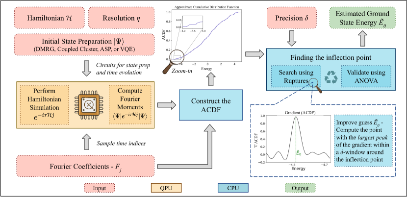
Figure 3: Workflow of the algorithm: The procedure takes as inputs the Hamiltonian $\mathcal{H}$, initial state $|\psi\rangle$ and tolerance parameters $\delta$ and $\eta$. The Fourier moments, see Eq. (11), are computed on the quantum computer with time indices $j$ sampled based on the Fourier coefficients of the approximate error function. The approximated CDF is built by summing the moments with the coefficients, as shown in Eq. (10). Finally, the ground state energy $\tilde{E}_{0}$ is predicted by first finding the inflection point using ruptures, validated by the ANOVA scheme, as an initial guess and improving upon it with the point with the maximal gradient in its $\delta$-neighbourhood (Sec. III.3).

Finally, to bring the convergence from $\mathcal{O}(\epsilon^{-2})$ down to $\mathcal{O}(\epsilon^{-1})$, and therefore reach the Heisenberg scaling limit, the sum can be computed using importance sampling [28]. More precisely, a set of $M$ values $\{k_{1},\dots,k_{M}\}\subset\{1,2,\dots,\lceil(D-1)/2\rceil\}$ is first sampled, where $k\sim|F_{k}|/\mathcal{F}$ and the normalization factor $\mathcal{F}=\sum_{k=1}^{d}|F_{2k+1}|$. The approximate CDF (ACDF) is then given by the average

$$\begin{split}G(x)=\frac{1}{2}+\frac{2\mathcal{F}}{M}\sum_{i=1}^{M}\Big{[}&\real[g_{k_{i}}(\tau)]\sin{(k_{i}x)}\\ +&\imaginary[g_{k_{i}}(\tau)]\cos{(k_{i}x)}\Big{]}.\end{split}$$ (13)

Following the same steps as in [28], one can easily show that the variance of $G$ is bounded by $2\mathcal{F}^{2}/M$. Once an estimate $\tilde{E}$ is found, we can refine it by computing the derivative of the ACDF and take the maximum on an interval $[\tilde{E}-\delta,\tilde{E}+\delta]$ of the CDF’s derivative [35]

$$\begin{split}G^{\prime}(x)=\frac{2\mathcal{F}}{M}\sum_{i=1}^{M}k_{i}\Big{[}&\real[g_{k_{i}}(\tau)]\cos{k_{i}x}\\ -&\imaginary[g_{k_{i}}(\tau)]\sin{k_{i}x}\Big{]}.\end{split}$$ (14)

We note that this is similar in spirit to identifying the maxima of a Gaussian kernel placed around the energy guess $\tilde{E}$ [33]. An overview of the whole algorithm is shown in Fig. 3, with input parameters, reconstruction of ACDF and the detection of inflection point, which we cover in greater detail in the next section.

III The LT algorithm in practice

The LT algorithm is a candidate ground-state energy estimation algorithm for early fault-tolerant quantum computing (FTQC) devices. Even though it is proven that this algorithm can find the ground-state energy using $M=\mathcal{O}(1/\eta^{2})$ samples and maximal depth $D=\mathcal{O}(\delta^{-1}\log{\delta^{-1}\eta^{-1}})$ [28], several challenges must be overcome for it to be useful in realistic settings. In this section, we identify these practical problems and propose implementable solutions. Most of them arise from the assumption that we have access to an initial state with at least $\eta$ overlap with the actual ground state, with $\eta$ large enough. However, this is not realistic in general for the following reasons: (i) it is difficult to prepare initial states with significant overlaps, and (ii) there is a lack of techniques to estimate the bound $\eta$ on the overlap parameter $p_{0}$.

III.1 Initial state preparation

The quality of the initial state significantly constrains the efficacy of quantum phase estimation (QPE) and its variants, specifically its overlap with the true ground state. Therefore, the method employed to prepare the initial states plays a pivotal role. In this regard, the two primary approaches involve evolving a known quantum state via quantum techniques or directly loading a wave function obtained via classical methods.

Adiabatic state preparation (ASP) methods have been widely studied to prepare ground-states [46]. They encompass advancements such as shortcuts to adiabaticity [47], counterdiabatic driving techniques [48, 49, 50], or hybrid approaches like counterdiabatic optimal local driving [51, 52]. Additionally, VQE [6] and dissipative [53, 54, 55, 56, 57] methods have some prospects. However, the scalability of these techniques to large system sizes remains to be determined. For instance, ASP demands an evolution time inversely proportional to the spectral gap, which can be exponentially small. Conversely, VQE is plagued by issues of trainability [22], particularly concerning the barren plateau phenomenon [23, 21] and high sample complexity [58]. Finally, dissipative methods require coupling to a bath or transformations of the Hamiltonian using quantum signal processing, which can be expensive to implement.

The second category comprises techniques that load state vectors, given in a classical representation obtained by methods such as DMRG [42, 43] and coupled cluster (CC) [59], directly on the quantum computer. These techniques offer a crucial advantage by introducing cutoff parameters, such as the bond dimension $\chi$ for DMRG or the number of interacting orbitals for CC. Despite their steep scaling with system size, it is always feasible to identify an affordable cutoff that makes these methods implementable in practice. Generally, this yields a state far superior to a random guess or a mean-field state like Hartree-Fock, enabling the extraction of low-lying eigenstate components using approaches like LT or QPE. An important step when using classical techniques is the loading of the obtained state onto the quantum computer. In fact, if the state vector is arbitrary, the cost is typically exponential in the number of qubits, e.g., using the scheme by Möttönen et al. [60]. Better scaling can be achieved if the state exhibits some special properties. For example, Refs  [61, 37] developed a method to load multi-Slater determinants and CC states, respectively. On the other hand, states obtained via DMRG can be loaded with overhead at most polynomial in the bond dimension [62, 63, 64, 65]. As an extra step, we note that techniques have been introduced to further enhance initial state overlap, for example by optimizing the set of orbitals [66], or filtering out undesirable contributions [67], while heuristics are provided in Ref. [68].

1

Input: signal $\{y_{i}\}_{i=1}^{n}$, failure probability $\alpha\in[0,1]$

FindBP(y, $\alpha$) ;

  $\triangleright$ Finds breakpoint (Eq. 17)

$b\leftarrow n$ ;

2 significant $\leftarrow$ True ;

3 while significant do

       $\tilde{b}=\textnormal{{FindBP}}(y[:b],\ \alpha)$ ;

        $\triangleright$ Optimization

       significant = ANOVA $(y,\ b,\ \alpha)$ ;

        $\triangleright$ Validation

4       if significant then

             $b\leftarrow\tilde{b}$ ;

              $\triangleright$ Upon successful validation

5            

6      

Output: $b$

Algorithm 1 Find smallest breakpoint

We instead choose to address this challenge by sparsifying (or truncating) the classical wavefunction and using the sparse quantum state preparation proposed by Gleinig and Hoefler [44]. The sparsification procedure consists of retaining only the $S$ largest components, setting all others to zero, and renormalizing. This $S$-sparsified state, denoted as $|\Psi_{S}\rangle$, can be efficiently loaded on the quantum computer, using only $\mathcal{O}(SN)$ two-qubit gates and $\mathcal{O}(S\log{S}+N)$ single-qubit gates, circumventing exponential scaling. Even if DMRG states can be loaded with only a polynomial overhead in the bond dimension [62, 63, 64, 65], the sparsification procedure might be useful in the case that the prefactor is still significantly high. Moreover, sparsifying the state enables us to probe the regime where DMRG does not converge and serves as a proxy to study the LT algorithms would perform in this scenario.

III.2 Hamiltonian simulation

It’s customary to quantify resource requirements in terms of calls to the time evolution oracle $\mathcal{U}(n\tau)$. However, a practical implementation necessitates an understanding of how to drive the dynamics efficiently. In order to keep the Heisenberg scaling, it is necessary to use asymptotically optimal methods based on linear combinations of unitaries (LCU) and qubitization [69, 70], generally scaling as $\mathcal{O}(\norm{\mathcal{H}}_{1}\tau D+\log{\epsilon^{-1}})$ queries to the LCU decomposition. However, they come with significant drawbacks, such as requiring multiple ancillary qubits, high connectivity and a usual high pre-factor. Therefore, we opt to utilize product formulas (PF) based on $p$-order Trotter-Suzuki decomposition [71], with an error scaling as $\epsilon\leq C(\tau D)^{p+1}/r^{p}$, and $r$ the number of Trotter steps and $C$ a prefactor depending on the commutators [72], which can be determined specifically for each system, e.g. spins [4], the Hubbard model [73] or neutrinos [74]. This choice is motivated by two key factors: firstly, PFs do not entail ancilla overhead or costly control operations, and they often outperform what is theoretically guaranteed, even when limited to the low-energy regime [75]. To contain the error below $\epsilon$, we can choose

$$\begin{split}r&=\left\lceil C^{1/p}(\tau D)^{(1+1/p)}\epsilon^{-1/p}\right\rceil.\end{split}$$ (15)

By doing so, we lose the Heisenberg scaling but retain quantum circuits that are resilient to the restrictions of early FTQC devices in the sense that they do not require expensive operations. In fact, for $d$-local Hamiltonians, PFs can leverage vanishing commutators and achieve better scaling than using qubitization, at least when the desired error is above some threshold. Moreover, since the Fourier coefficients decay as $1/x$, we are more likely to run short-time simulations, which is the strong suit of PFs. This intuition is supported by our numerical experiments in Sec. V, where good energy estimation is obtained even for circuits constrained to relatively low depths.

Although we do not explicitly delve into these techniques, various enhancements for product formulas exist, including but not limited to randomization [76, 77, 78], multi-product formulas [79, 80], qDRIFT compilation [81, 82, 83, 84], and composite formulas [85, 86]. Since those techniques trade the circuit’s depth with additional measurements, they are well suited for early FTQC, warranting further investigation in more targeted studies.

Input: signal $\{y_{i}\}_{i=1}^{n}$, breaking point $b\in[1,n]$, failure probability $\alpha\in[0,1]$

$\bar{y}=\frac{1}{n}\sum_{i=1}^{n}y_{i}$ ;

  $\triangleright$ Mean of signal components

$\bar{y}_{0}=\frac{1}{b}\sum_{i=1}^{b}y_{i}$ ;

  $\triangleright$ Mean of first segment

$\bar{y}_{1}=\frac{1}{n-b}\sum_{i\geq b}y_{i}$ ;

  $\triangleright$ Mean of second segment

$SS_{w}=\sum_{i=1}^{n}(y_{i}-\bar{y})^{2}$ ;

  $\triangleright$ Sum of squares within segments

$SS_{b}=\sum_{i<b}(y_{i}-\bar{y}_{0})^{2}+\sum_{i\geq b}(y_{i}-\bar{y}_{1})^{2}$ ;

  $\triangleright$ Sum of squares between segments

$f=(n-2)SS_{b}/SS_{w}$ ;

  $\triangleright$ F-ratio

1 significant $\leftarrow$ False ;

2 if $F(f,1,n-2)>(1-\alpha)$ then

3      if $\bar{y}_{1}>\bar{y}_{0}$ then

             significant $\leftarrow$ True ;

              $\triangleright$ Successful F-test & monotone function

4            

5       end if

6      

7 end if

Output: significant $\in$ {True, False}

Algorithm 2 ANOVA

III.3 Detection of discontinuities

The second main challenge we face is the detection of the discontinuities in the ACDF, which is directly related to the difficulty of computing a tight lower bound $\eta$ on the overlap with the true ground state. The problem is twofold: (i) having access to an upper bound $\eta$ that describes the size of the jump and is required to invert the CDF as described in [28] is difficult, and (ii) since the number of jumps grows exponentially with the system size, the CDF becomes quasi-continuous, making any jump detection difficult. This can already be seen from Fig. 1, where the CDF with eight qubits looks much smoother than with four. This is tightly related to the orthogonality catastrophe [87, 2, 88], stating that the overlap between a random initial state and any eigenstate vanishes exponentially fast for larger systems. We note that the continuous nature of the CDF is driven by the size of the support of the initial state in the eigenbasis. Hence, bound states, or more generally states which are sparse in this basis, will lead to clear step functions. However, since preparing initial states of this quality remains an open problem, it is important to consider states with exponential support.

We adopt a different perspective, seeking to understand the practical implications of employing LT with an initial state of unknown quality. Rather than striving for the exact determination of the ground state energy, we focus on enhancing the energy estimate of the initial state. To this end, we aim to locate the inflection point of the CDF, which is generally lower than the energy expectation value of the initial state yet still provides an upper bound on the ground-state energy. We address this new task by identifying a statistically significant increase in the ACDF comprised of small contributions from neighbouring eigenstates. More precisely, we replace the overlap with the true ground state by the overlap’s accumulation in the low-energy regime

$$\eta=\sum_{i<m}|\langle E_{i}|\Psi\rangle|^{2},$$ (16)

where $m$ is a truncation parameter related to the desired resolution.

We propose a procedure based on a kernel change-point detection method [89, 90]; this is a signal processing technique to detect changes in the mean of a given signal, implemented with the software package ruptures [91]. Despite its simplicity, the technique can be used to perform complex time series analysis, yielding great results across multiple scientific domains [92, 93, 94, 95]. In this scenario, we execute an iterative procedure (Algorithm 1) that comprises two primary steps: (i) dividing the signal into two segments, which entails identifying the breakpoint that optimally separates the time series, and (ii) evaluating the statistical significance of the split using the ANOVA-based scheme. If so, we repeat these steps on the early (left) part of the signal up to the recently detected split, finding new breakpoints closer to the initial point with every iteration until one is rejected. In other words, we aim to find the inflection point of the CDF, i.e., the zero of its second derivative.

To find the breakpoint, the signal $y$ is first mapped onto a reproducing Hilbert space with $\phi:\mathbb{R}\rightarrow\mathbb{H}$, implicitly defined as $\phi(y)=K(y,\cdot)$. The kernel function $K$, typically chosen to be Gaussian, induces the metric on the Hilbert space. We then solve the following minimization problem to find the smallest breakpoint:

$$\min_{b\in\{1,\ldots,n\}}\ \sum_{t=1}^{b}\norm{\phi(y_{t})-\bar{y}_{1:b}}+\sum_{t=b+1}^{n}\norm{\phi(y_{t})-\bar{y}_{b+1:n}},$$ (17)

where $\bar{y}_{a:b}=\sum_{x=a}^{b}y_{x}/(b-a)$ is the mean of the signal between $a$ and $b$. We guide the reader to Ref. [89] for an in-depth description of this technique.

The ANOVA algorithm (Algorithm 2) decides if the breakpoint is statically significant by computing the mean of the two segments, as well as their standard deviations and their ratio $f$. The breakpoint is accepted if the $p$ value of an F-test [96] with input $(f,1,n-2)$ is greater than $1-\alpha$, with $\alpha$ being a small permissible failure probability. We recall that the F-test is a statistical test for comparing the variances or standard deviations from two populations using the F-distribution. Since we require the CDF to be monotone increasing, the breakpoint $b$ is only accepted if $\bar{y}_{1:b}>\bar{y}_{b+1:n}$, in addition to passing the F-test.

Furthermore, we avoid overshooting by stopping the procedure if the left part of the breakpoint is, on average, smaller than a threshold. To this end, we stop the point search if $\bar{y}_{b-l:b}>k\sigma+\tilde{\epsilon}$, for $k\in\mathbb{N}$, $l$ a small window (for example, $l=20$), and $\sigma$ and $\tilde{\epsilon}$ are the empirical standard deviation and error, respectively, of the signal computed on the energy region $-\pi\leq x<-\pi/2$, where we know that no eigenvalues are present. Using these empirical estimates has the advantage of being closer to the truth than the theoretical upper bounds while being available at no additional cost. The value of $k$ sets the confidence of the predictions and is usually chosen as $k\in\{1,2,3\}$. In order to make the scheme more robust, we repeat the above procedure multiple times using different data for the ACDF and compute the median of means. Once the inflection point $\tilde{b}$ is known, the energy guess is chosen as the maxima of the gradient of the ACDF around a small window $\delta$ around the inflection point, $[\tilde{b}-\delta/2,\ \tilde{b}+\delta/2]$, as depicted in Fig. 3.

In summary, the signal is processed using ruptures to find a breakpoint, which is then validated according to a statistical test subject to a monotone function condition. If accepted, we perform the same analysis on the early part of the signal up to the breakpoint and discard the rest. We repeat these steps until a breakpoint is discarded and take the last valid breakpoint as a guess for the inflection point of the CDF. Since the eigenvalue is situated at the middle of the jump, it is important to look at the gradient of the CDF. The first significant maximum of the gradient exactly corresponds to an eigenvalue, while the secondary peaks are due to the approximation with the Fourier series. The whole procedure described in this section can be summed up as following steps -

1. Prepare the best possible ground state $|\Psi\rangle$ using the available methods in your toolbox, e.g., DMRG  [42], coupled cluster (CC) [59], etc.

2. Load the state on the quantum computer, e.g., by sparsification [44], or by encoding them as sums of Slater determinants or matrix-product states (MPS) [37].

3. Sample $M$ time indices from the coefficients of the Fourier series [Eq. (6)].

4. Use a product formula to compute one sample of the corresponding Fourier moment with a suitable number of steps [Eq. (15)].

5. Build the approximate CDF (ACDF) using $M$ samples [Eq. (13)].

6. Identify the inflection point $x$ of the ACDF using ruptures [Eq. (17)].

7. The energy estimate is the maxima of the ACDF’s derivative in an $\delta$-window around $x$.

IV Resources estimates

In light of the challenges that stem from implementing the LT algorithm in practice, especially obtaining tight lower bounds $\eta$, and the potentially small overlap between the initial state and the target ground state, we strive to find what is the best that can be done using limited resources. More precisely, we tackle the following problem.

Problem 2.

Given a maximal depth $D$ and a maximal shot budget $M$, what is the best upper bound on the ground-state energy that can be provided by the algorithm?

In this section, we provide quantitative resource estimates of the LT algorithm, which falls into two categories — the highest Fourier moment $D$, which is related to the maximal evolution time of the Hamiltonian simulation via $T_{\text{max}}=\tau D$, responsible for the bias in approximating the ACDF, and the number of samples $M$, which is associated with the variance of the output energy. We note that $D$ is directly linked to the maximal depth of the quantum circuits, which is why we also relate to it as maximal runtime.

Theorem 1.

For a given accuracy $\epsilon\in(0,1)$, the maximal runtime $D$ required to approximate the error function $\erf{(\cdot)}$ with $\epsilon$-error is given by

$$D=2\cdot\left\lceil\sqrt{f\left(\beta,\,\min{\left[1,\ 4e^{-w(\epsilon)/2}\right]}\right)\cdot w(\epsilon)}\ \right\rceil+1,$$ (18)

where $\beta$ is chosen according to Eq. (7) and

$$\begin{split}w(\epsilon)&=W_{0}\left(\frac{18}{\pi\epsilon^{2}}\right),\\ f(\beta,\epsilon)&=-\frac{\ln{\epsilon}+\beta}{W_{0}\left(-\left[1+\beta^{-1}\ln{\epsilon}\right]e^{-1}\right)}\ ,\\ \end{split}$$ (19)

with $W_{0}(\cdot)$ being the principal branch of the Lambert-W function.

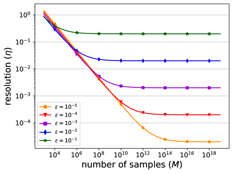
Figure 4: Estimating the resolution. Estimation of the resolution $\eta$ of a jump that can be resolved for the case of 26 spins fully connected Heisenberg model discussed in Sec. V.2, using a given number of samples $M$ with $1-\vartheta=95\%$ confidence for different precision parameters $\epsilon$.

Proof.

The proof of this theorem can be based on Ref. [32, Theorem 3, Appendix A], which describes a Fourier approximation to the Heaviside function as $\max|\Theta(x)-F(x;\beta)|\leq(\epsilon_{1}+\epsilon_{2}+\epsilon_{3})/2=\epsilon$  [32, Eq. (A12)], where $\epsilon_{\{1,2\}}$ are the errors due to finite truncation $d$ and scaling parameter $\beta$, respectively, in approximating the error function using Eqs. (5, 6), and $\epsilon_{3}$ is the error in approximating the Heaviside function with an error function. For the choice $\epsilon_{1}=\epsilon_{2}=\epsilon_{3}=2\epsilon/3$ in this approximation, and using the values of $\beta$ and $d$ such that of $-(\epsilon_{1}+\epsilon_{2})/2\leq F_{d}(x,\beta)\leq 1+(\epsilon_{1}+\epsilon_{2})/2$  [32, Eq. (A13)], we get $d\geq\sqrt{t\cdot w(\epsilon)}$ [32, Eq. (A6)] for an integer $t$ where

$$t=\begin{cases}f(\beta,\,4e^{-w(\epsilon)/2})&\text{for}\ w(\epsilon)\geq 2\ln 4\\ \beta&\text{for}\ w(\epsilon)<2\ln 4\\ \end{cases},$$ (20)

with the function $f(\cdot,\cdot)$ defined above. Since $f(\beta,1)=\beta$ and $\epsilon\in(0,1)$, one can rewrite Eq. (20) as $t=f(\beta,\,\min\left[1,\,4e^{-w(\epsilon)/2}\right])$ and obtain the minimum maximal runtime $D=2d+1$ as $2\left\lceil\sqrt{t\cdot w(\epsilon)}\,\right\rceil+1$. ∎

One can then use this maximal runtime for the estimation of the number of samples that are required to resolve an accumulation of size $\eta$. It is important to note that $\eta$ is no longer a lower bound on the overlap but a parameter chosen by the user, quantifying the desired resolution.

Theorem 2.

For a given maximal runtime $D$ and accuracy $\epsilon\in(0,1)$, the number of samples $M$ required to guarantee the correct result with probability $1-\vartheta$ is

$$\begin{split}M=&\Bigg{\lceil}2\cdot\left[\frac{2.07\pi^{-1}(\log{4D}+\gamma)+1}{\eta-2\epsilon}\right]^{2}\cdot\\ &\left[\log{\log{\left(\frac{1}{\tau\epsilon}\right)}+\log{(\vartheta^{-1})}}\right]\Bigg{\rceil},\end{split}$$ (21)

where $\eta>2\epsilon$ is the accumulation on the low-energy part of the spectrum and $\gamma$ is the Euler-Mascheroni constant. The last assumption is required since a jump smaller than the error threshold cannot be resolved.

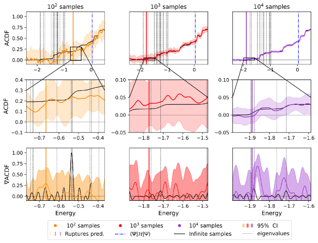
Figure 5: Six spins, random initial state. ACDF (top row), zoom ACDF (middle row) and its gradient ($\nabla$ACDF, bottom row) computed with different number of samples (each column). The first 20 eigenvalues obtained from exact diagonalization are reported with dashed vertical lines, while the thick blue vertical line shows the energy of the initial state. The coloured line represents the energy found with the ruptures procedure. The black line shows the ACDF (and its gradient) computed with infinite statistics, while the shaded area is a 95% confidence interval computed with ten repetitions.

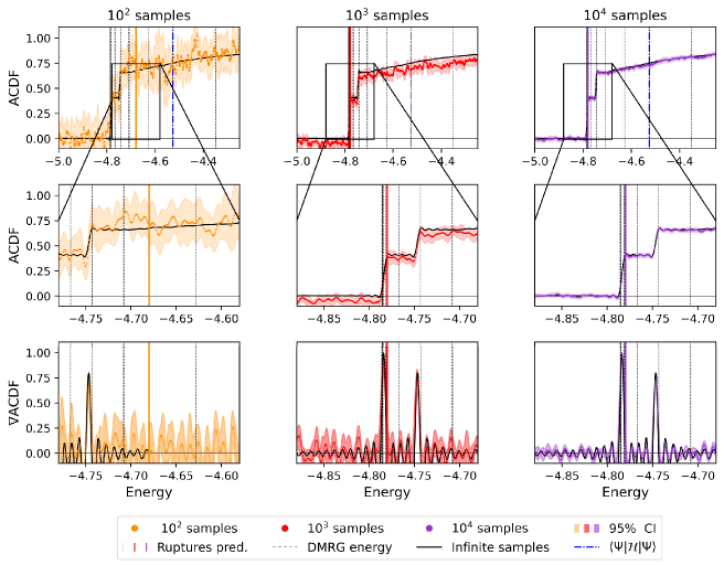
Figure 6: 26 spins, DMRG ($\mathbf{\chi=10}$). ACDF (top row), zoomed ACDF (middle row) and its gradient ($\nabla$ACDF, bottom row) computed with the different numbers of samples (each column). The energies obtained with untruncated DMRG states with different bond dimensions $5\leq\chi\leq 2000$ are reported with dashed vertical lines, while the thick blue vertical line shows the energy of the initial state. The coloured line represents the energy found with the ruptures procedure. The black line shows the ACDF (and its gradient) computed with infinite statistics, while the shaded region is a 95% confidence interval computed with ten repetitions.

Proof.

We make use of $\mathbb{E}[G]=\tilde{C}(x)$ from Eq. $\eqref{eq:acdf_def}$ to decide the Problem 1 from Eq. $\eqref{eq:prob_1}$ as:

$$\begin{split}G<\zeta\ &\Rightarrow\ \mbox{Tr}[\rho\Pi_{\leq x-\delta}]<\eta\\ G\geq\zeta\ &\Rightarrow\ \mbox{Tr}[\rho\Pi_{\leq x+\delta}]>0.\end{split}$$ (22)

We use $\zeta=\eta/2$ to attune for errors in estimating $G(x)$ from sampling (Eq. (13)) and decide whether $\tilde{C}(x)=0$ or $\tilde{C}(x)\geq\eta$. Consequently, we can define the above as the probability $\mathbb{P}[G<\eta/2]<\kappa$ conditioned on $\tilde{C}(x)<\eta-\epsilon$ which implies $C(x-\delta)<\eta$, and use the one-sided Chebyshev inequality to find

$$\begin{split}\mathbb{P}[G<\eta/2]&<\mathbb{P}[G\leq\eta/2]\\ &=\mathbb{P}[G\leq\tilde{C}-\eta/2+\epsilon]\\ &\leq\frac{\mbox{Var}[G]}{\mbox{Var}[G]+\left(\eta/2-\epsilon\right)^{2}}\\ &<\frac{\mbox{Var}[G]}{\left(\eta/2-\epsilon\right)^{2}}\;.\end{split}$$ (23)

Using the upper bound on the variance of $G$ discussed after Eq. (13) above we finally obtain

$$\mathbb{P}[G<\eta/2]<\frac{8\mathcal{F}^{2}}{M(\eta-2\epsilon)^{2}}\;,$$ (24)

and in order to guarantee that this probability will be bounded by $\kappa$ we can then take

$$M\geq\left(\frac{2\sqrt{2}\mathcal{F}}{\eta-2\epsilon}\right)^{2}\left(\frac{1}{\kappa}\right)\;.$$ (25)

We can improve the dependence on $\kappa$ by using the fact that the individual summands in the average that defines $G$ are bounded by $2\mathcal{F}/M$ which allows us to employ the Hoeffding inequality as follows

$$\begin{split}\mathbb{P}[\bar{G}<\eta/2]<&\exp\left(-\frac{2\cdot\left(\eta/2-\epsilon\right)^{2}}{M\cdot(2\mathcal{F}/M)^{2}}\right)\\ &\Rightarrow M\geq\left(\frac{2\sqrt{2}\mathcal{F}}{\eta-2\epsilon}\right)^{2}\log\left(\frac{1}{\kappa}\right)\;.\end{split}$$ (26)

We can now use the upper bound for the norm of the Fourier coefficients $\mathcal{F}$ computed as [32]:

$$\begin{split}\mathcal{F}=\sum_{|j|\leq d}|\hat{F}_{j}(\beta)|&\leq\frac{2.07}{2\pi}(H_{D}+2\ln{2})+\frac{1}{2}\\ &\approx\frac{2.07}{2\pi}\left(\log(4D)+\gamma\right)+\frac{1}{2},\end{split}$$ (27)

where $H_{k}$ denotes the k${}^{\text{th}}$ Harmonic number, which can be estimated as done above using the Euler-Mascheroni constant $\gamma=0.57721567$ [97].

Finally, we can get the provided result by noting that Algorithm 1 needs to be run $\mathcal{O}(\log\delta^{-1})$ times to solve Problem 1 [28], and if it fails with probability at most $\kappa$ then to successfully estimate the ground state of the system with probability $1-\vartheta$ we would have $\kappa^{-1}\leq\vartheta^{-1}\log\delta^{-1}$, with $\delta=\tau\epsilon$ as before.

∎

It is important to note that these estimates are meant to be used in estimating the error tolerance and resolution which can be achieved using limited resources $D$ and $M$. For instance, we use the Theorem 2 in Fig. 4 to show the inflections of size $\eta$ that can be resolved for different error tolerances $\epsilon$ with a given sample budget $M$. We observe that the resolution which can be achieved plateaus after a certain sample budget, meaning that for further refined resolution, we need to increase the simulation time (i.e., decrease $\epsilon$). In particular, this means that we can not trade depth with samples indefinitely, and that to reach higher resolution, it is required to increase the depth. As stated in Theorem 1, the maximum depth $D$ is primarily determined by the error $\epsilon$ when approximating the step function. This implies that considerable depth is required to detect even a minor accumulation in the CDF. However, if the initial state predominantly occupies the lower-energy eigenstates, the accumulation may be significant enough to be identified within a constrained maximum depth. For instance, aiming for a 1% error ratio may be sufficient for most applications and can be detected within a realistic maximum depth. We will now delve deeper into this observation by conducting numerical simulations on a challenging system.

Figure 7: 26 spins, sparsified DMRG ($\mathbf{\chi=10}$). ACDF (top row), zoomed ACDF (middle row) and its gradient ($\nabla$ACDF, bottom row) computed with the different numbers of samples (each column). The energies obtained with untruncated DMRG states with different bond dimensions $5\leq\chi\leq 2000$ are reported with dashed vertical lines, while the thick blue vertical line shows the energy of the sparsified initial state with $S=13$. The coloured line represents the energy found with the ruptures procedure. The black line shows the ACDF (and its gradient) computed with infinite statistics, while the shaded region is a 95% confidence interval computed with ten repetitions.

V Numerical simulations

We consider a fully connected Heisenberg model with random couplings over $N$ spins

$$\begin{split}\mathcal{H}&=\frac{1}{N}\sum_{i<j}\sum_{a\in\{x,y,z\}}J_{a}^{ij}\cdot\sigma_{a}^{i}\sigma_{a}^{j},\text{ where }J_{a}^{ij}\sim\mathcal{N}(0,1).\end{split}$$ (28)

Here, $\sigma_{a}^{i}$ is the corresponding Pauli matrix applied to the $i$-th qubit. This model is gapless in general and universal, in the sense that it can approximate any two-local Hamiltonian [98]. Moreover, the tensor network techniques are not expected to perform well due to the high number of connections, making it a good testbed for quantum algorithms. For this system, we simulate the dynamics using a second-order Trotter-Suzuki formula [71] with time step $\Delta t=\tau/r$, with $r=8$ being the number of Trotter steps, and a SWAP networks-based [99, 100] circuit construction to obtain the most compressed circuits as possible.

Using a product formula for approximating the time evolution has the advantage of keeping the circuit shallow, being, therefore, more suited for early FTQC devices. For instance, the depth of the quantum circuits used in the following reads $2NrD$. We note that we did not use any of the potential improvements to Hamiltonian simulation with product formulas discussed in Sec. III.2, which are likely to decrease the maximal depth at the expense of additional samples.

V.1 Small system sizes

We start with a small system with six spins ($N=6$). We choose a random initial state with $p_{0}=0.0014$ and $p_{1}=0.015$. Note that this is a state of poor quality, compared to DMRG. We also set $\epsilon=0.055$ and therefore require $D=350$ Fourier moments for constructing the ACDF.

Both the ACDF and its gradient are shown in Fig. 5 for different numbers of samples. The continuous black line, referred to as the infinite statistics limit, corresponds to the infinite samples regime, where the moments are exact, and all of them, up to $D$, are included in the approximation. The ground-state energy is estimated with the procedure introduced in Sec. III.3, in which we first find an approximate guess for the inflection point and then refine it by taking the maximum of the gradient around it. We observe that we are not able to find the ground state, which is due to the approximation error of the step function $\epsilon$ being larger than the overlap. However, we are able to find the first excited-state energy using only $10^{4}$ shots and a random initial state. We note that we are able to find the energy of the true ground state using a better initial state, e.g. a DMRG state of low bond dimension.

V.2 Large system sizes

We then move to a larger model composed of $N=26$ spins. Since exact diagonalization is too expensive, in this regime, we refer to DMRG with bond dimension $\chi=2000$ to obtain the target energy. We choose $\epsilon=0.019$, translating into $D=6600$. We perform two experiments: the first starting from $|\Psi\rangle=\text{DMRG}(\chi=10)$, and the second from its sparsification with $S=13$. The motivation to use DMRG with low bond dimension is to have a good initial state, which can be computed even for large system sizes.

The results with the DMRG state are shown in Fig. 6, which displays the ACDF computed with $10^{2}$, $10^{3}$ and $10^{4}$ samples. The data displays the two main contributions from low-level energy eigenstates and a continuous contribution from higher states. With our procedure, we can recover the ground-state energy equivalent to DMRG with $\chi=2000$ from the gradient of the ACDF. An important point to make at this stage is that the CDF clearly exhibits two jumps on the low-lying part of the spectrum. This is due to the high quality of the initial state, which consists of two bound states of low energy and a tail of high-energy residuum. Therefore, the left part of the CDF exhibits a step-like shape, while the right part is continuous. However, as seen in Fig. 7, the CDF obtained from the sparsified DMRG state looks continuous, and we only unravel discontinuities when magnifying by a factor of one hundred. The important point is that in both cases, we improve on the DMRG estimate (blue dotted vertical line), by $5\%$ and $32\%$ respectively.

The key difference with respect to the above case, is that the ACDF does not display any clear steps and, as such, we have to rely on finding the inflection point. This results in the need of more samples to find the ground state energy, requiring $10^{5}$ and $10^{7}$ samples to recover the energy of DMRG with $\chi=1000$ and $\chi=2000$, respectively. To study the quality of the sparsified initial state $|\Psi_{S}\rangle$, we show the $L^{2}$ distance and the overlap with the true DMRG initial state as a function of the truncation parameter $k$ in Fig. 8. We observe that the quality increase slows down after $S=13$, which is the reason this truncation was chosen. Furthermore, we note that the overlap squared $p_{0}$ between the (sparsified) initial state and the converged DMRG state reads ($2\times 10^{-5}$) $7\times 10^{-6}$, requiring $M=10^{13}$ (using Theorem 2) samples to distinguish the exact ground state with $95\%$ certainty. This is why we should instead search for inflection points since it requires several orders of magnitude less resources than what is expected theoretically from detecting discontinuities while achieving similar performance. The important point here is the change of paradigm, going from aiming at the true ground-state energy, which is challenging and costly, to detecting a relevant accumulation, which is much cheaper and is usually good enough for most applications.

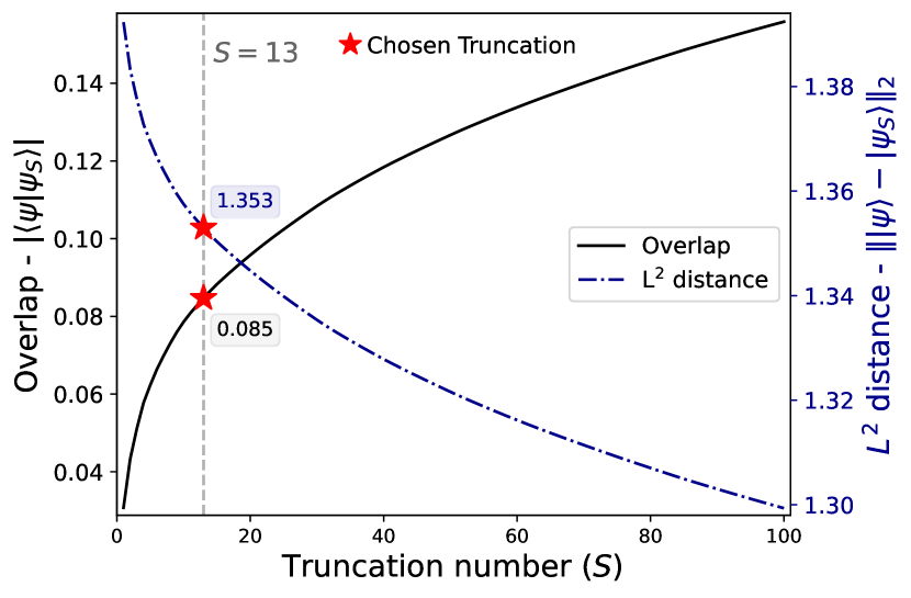
Figure 8: Quality of the sparsification The left axis (black) shows the overlap of $|\Psi_{S}\rangle$ with the full DMRG initial state, while the right axis (blue) shows the corresponding L² distance. The red stars correspond to the truncation number chosen for the experiments.

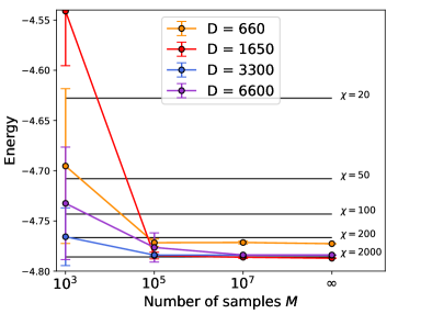
((a))

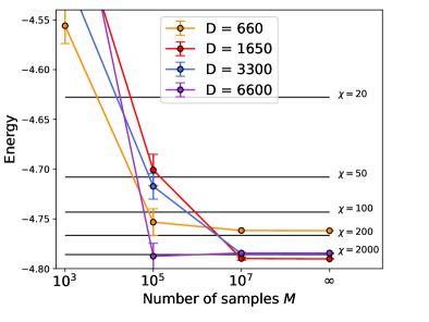
((b))

Figure 9: Energy predictions using the method introduced in Section III.3 taking the maxima of the gradient of the ACDF in a $\delta=0.01$ window. The horizontal lines depict the values predicted by DMRG with different bond dimensions $\chi$. The different colours refer to the maximum time evolution used to compute the ACDF, while the x-axis depicts the number of samples. The error bars represent one standard deviation computed over ten experiments. The infinity symbol refers to the regime of infinite samples.

Finally, we show the energy predictions as a function of the number of samples and maximal depth in Fig. 9. We observe that with only a fifth of the depth considered in the previous experiments, we can already obtain the same energy estimates using just $10^{3}$ and $10^{5}$ samples, respectively, for the full and sparse initial states. This hints that finding the inflection point requires less precision than a jump, thus that fewer moments are required, in practice.

VI Conclusion

In this paper, we examine the practical performance of early fault-tolerant algorithms for ground-state energy estimation. Specifically, our focus here has been on the Lin and Tong (LT) algorithm [28], which approximates the cumulative distribution function (CDF) of the spectral measure and associates its discontinuities with the eigenvalues of the corresponding Hamiltonian. Notably, this algorithm requires only one ancillary qubit and the ability to perform real-time evolution, making it a promising candidate for the intermediate-scale quantum hardware. We have summarized the current state-of-the-art setup of this algorithm and make three distinct contributions there to enhance its practicality: the identification of the relevant challenges appearing in practice and how to address them; quantitative resource estimation in terms of maximal shot budget and evolution time for Hamiltonian simulation; and numerical simulation on a non-trivial system. We advocate using product formulas for time evolution, even if we lose the Heisenberg scaling by doing so. Hence, they enjoy low implementation overhead and are likely better for the short-time evolution of local Hamiltonian, rather than the asymptotically optimal but more expensive techniques.

In light of the numerical simulation performed on the challenging fully-connected, fully-random Heisenberg model, LT-type algorithms emerge as a viable option for early fault-tolerant quantum (FTQ) devices. The key point was to change our mindset from aiming at the actual ground-state energy, which requires high depth and a number of samples, to instead concentrating on finding the spectral CDF’s inflection point. Moreover, suppose the initial state is of high enough quality, as seems to be the case for a (sparsified) DMRG state of low bond dimension. In that case, the inflection point lies close enough to the true energy and is usually precise enough for most applications. This paradigm change has the advantage of relaxing the requirement in the approximation error, which is responsible for scaling the depth and number of samples. While quantum phase estimation is still likely outperforming the LT algorithm in the FTQ computing era, our findings suggest that LT algorithms are able to improve on classical solutions, using only limited quantum resources ($10^{4}-10^{5}$ samples), orders of magnitude less than what is predicted by the theory. In conclusion, the LT algorithm emerges as a robust and efficient quantum algorithm, bridging the gap between NISQ and FTQ computing eras.

Code

We use Tenpy [101] for the DMRG calculations, PennyLane [102, 103] and Qsim [104] for the dynamics and Ruptures [91] for the breakpoint detection. Complete code is available upon request to the authors. Numerical experiments were performed on the CERN Openlab GPU cluster.

References

- Kempe et al. [2005] J. Kempe, A. Kitaev, and O. Regev, in FSTTCS 2004: Foundations of Software Technology and Theoretical Computer Science (Springer Berlin Heidelberg, 2005) pp. 372–383.
- Lee et al. [2023] S. Lee, J. Lee, H. Zhai, Y. Tong, A. M. Dalzell, A. Kumar, P. Helms, J. Gray, Z.-H. Cui, W. Liu, M. Kastoryano, R. Babbush, et al., Evaluating the evidence for exponential quantum advantage in ground-state quantum chemistry, Nature Communications 14, 10.1038/s41467-023-37587-6 (2023).
- Liu et al. [2022] H. Liu, G. H. Low, D. S. Steiger, T. Häner, M. Reiher, and M. Troyer, Prospects of quantum computing for molecular sciences, Materials Theory 6, 11 (2022).
- Childs et al. [2018] A. M. Childs, D. Maslov, Y. Nam, N. J. Ross, and Y. Su, Toward the first quantum simulation with quantum speedup, Proceedings of the National Academy of Sciences 115, 9456 (2018).
- Delgado et al. [2022] A. Delgado, P. A. M. Casares, R. dos Reis, M. S. Zini, R. Campos, N. Cruz-Hernández, A.-C. Voigt, A. Lowe, S. Jahangiri, M. A. Martin-Delgado, J. E. Mueller, and J. M. Arrazola, Simulating key properties of lithium-ion batteries with a fault-tolerant quantum computer, Phys. Rev. A 106, 032428 (2022).
- Peruzzo et al. [2014] A. Peruzzo, J. McClean, P. Shadbolt, M.-H. Yung, X.-Q. Zhou, P. J. Love, A. Aspuru-Guzik, and J. L. O’brien, A variational eigenvalue solver on a photonic quantum processor, Nature communications 5, 4213 (2014).
- Grimsley et al. [2019] H. R. Grimsley, S. E. Economou, E. Barnes, and N. J. Mayhall, An adaptive variational algorithm for exact molecular simulations on a quantum computer, Nature communications 10, 3007 (2019).
- Kiss et al. [2022] O. Kiss, M. Grossi, P. Lougovski, F. Sanchez, S. Vallecorsa, and T. Papenbrock, Quantum computing of the 6Li nucleus via ordered unitary coupled clusters, Physical Review C 106, 034325 (2022), publisher: American Physical Society.
- Uvarov et al. [2020] A. Uvarov, J. D. Biamonte, and D. Yudin, Variational quantum eigensolver for frustrated quantum systems, Phys. Rev. B 102, 075104 (2020).
- Grossi et al. [2023] M. Grossi, O. Kiss, F. De Luca, C. Zollo, I. Gremese, and A. Mandarino, Finite-size criticality in fully connected spin models on superconducting quantum hardware, Physical Review E 107, 024113 (2023), publisher: American Physical Society.
- Barkoutsos et al. [2018] P. K. Barkoutsos, J. F. Gonthier, I. Sokolov, N. Moll, G. Salis, A. Fuhrer, M. Ganzhorn, D. J. Egger, M. Troyer, A. Mezzacapo, S. Filipp, and I. Tavernelli, Quantum algorithms for electronic structure calculations: Particle-hole hamiltonian and optimized wave-function expansions, Phys. Rev. A 98, 022322 (2018).
- Feniou et al. [2023] C. Feniou, M. Hassan, D. Traoré, E. Giner, Y. Maday, and J.-P. Piquemal, Overlap-ADAPT-VQE: practical quantum chemistry on quantum computers via overlap-guided compact Ansätze, Communications Physics 6, 10.1038/s42005-023-00952-9 (2023).
- Azad and Singh [2022] U. Azad and H. Singh, Quantum chemistry calculations using energy derivatives on quantum computers, Chemical Physics 558, 111506 (2022).
- Dumitrescu et al. [2018] E. F. Dumitrescu, A. J. McCaskey, G. Hagen, G. R. Jansen, T. D. Morris, T. Papenbrock, R. C. Pooser, D. J. Dean, and P. Lougovski, Cloud quantum computing of an atomic nucleus, Phys. Rev. Lett. 120, 210501 (2018).
- Monaco et al. [2023] S. Monaco, O. Kiss, A. Mandarino, S. Vallecorsa, and M. Grossi, Quantum phase detection generalization from marginal quantum neural network models, Phys. Rev. B 107, L081105 (2023).
- Pérez-Obiol et al. [2023] A. Pérez-Obiol, A. Romero, J. Menéndez, A. Rios, A. García-Sáez, and B. Juliá-Díaz, Nuclear shell-model simulation in digital quantum computers, Scientific Reports 13, 12291 (2023).
- de Schoulepnikoff et al. [2024] P. de Schoulepnikoff, O. Kiss, S. Vallecorsa, G. Carleo, and M. Grossi, Hybrid ground-state quantum algorithms based on neural schrödinger forging, Phys. Rev. Res. 6, 023021 (2024).
- Sahoo et al. [2022] S. Sahoo, U. Azad, and H. Singh, Quantum phase recognition using quantum tensor networks, The European Physical Journal Plus 137, 10.1140/epjp/s13360-022-03587-6 (2022).
- Ralli et al. [2021] A. Ralli, P. J. Love, A. Tranter, and P. V. Coveney, Implementation of measurement reduction for the variational quantum eigensolver, Phys. Rev. Res. 3, 033195 (2021).
- Wecker et al. [2015] D. Wecker, M. B. Hastings, and M. Troyer, Progress towards practical quantum variational algorithms, Phys. Rev. A 92, 042303 (2015).
- Ragone et al. [2023] M. Ragone, B. N. Bakalov, F. Sauvage, A. F. Kemper, C. O. Marrero, M. Larocca, and M. Cerezo, A unified theory of barren plateaus for deep parametrized quantum circuits (2023), arXiv:2309.09342 [quant-ph] .
- Anschuetz and Kiani [2022] E. R. Anschuetz and B. T. Kiani, Quantum variational algorithms are swamped with traps, Nature Communications 13, 7760 (2022).
- Cerezo et al. [2021] M. Cerezo, A. Sone, T. Volkoff, L. Cincio, and P. J. Coles, Cost function dependent barren plateaus in shallow parametrized quantum circuits, Nature communications 12, 1791 (2021).
- Kitaev [1995] A. Y. Kitaev, Quantum measurements and the abelian stabilizer problem, arXiv e-prints (1995), arXiv:quant-ph/9511026 [quant-ph] .
- Preskill [2018] J. Preskill, Quantum Computing in the NISQ era and beyond, Quantum 2, 79 (2018).
- Liang et al. [2024] Q. Liang, Y. Zhou, A. Dalal, and P. Johnson, Modeling the performance of early fault-tolerant quantum algorithms, Phys. Rev. Res. 6, 023118 (2024).
- Somma et al. [2002] R. Somma, G. Ortiz, J. E. Gubernatis, E. Knill, and R. Laflamme, Simulating physical phenomena by quantum networks, Phys. Rev. A 65, 042323 (2002).
- Lin and Tong [2022] L. Lin and Y. Tong, Heisenberg-limited ground-state energy estimation for early fault-tolerant quantum computers, PRX Quantum 3, 10.1103/prxquantum.3.010318 (2022).
- Somma [2019] R. D. Somma, Quantum eigenvalue estimation via time series analysis, New Journal of Physics 21, 123025 (2019).
- Kiss et al. [2024] O. Kiss, M. Grossi, and A. Roggero, Quantum error mitigation for fourier moment computation, arXiv preprint arXiv:2401.13048 (2024).
- Cleve et al. [1998] R. Cleve, A. Ekert, C. Macchiavello, and M. Mosca, Quantum algorithms revisited, Proceedings of the Royal Society of London. Series A: Mathematical, Physical and Engineering Sciences 454, 339 (1998).
- Wan et al. [2022] K. Wan, M. Berta, and E. T. Campbell, A randomized quantum algorithm for statistical phase estimation, Physical Review Letters 129, 030503 (2022), arXiv:2110.12071 [quant-ph].
- Wang et al. [2023] G. Wang, D. S. França, R. Zhang, S. Zhu, and P. D. Johnson, Quantum algorithm for ground state energy estimation using circuit depth with exponentially improved dependence on precision, Quantum 7, 1167 (2023).
- Dong et al. [2022] Y. Dong, L. Lin, and Y. Tong, Ground-state preparation and energy estimation on early fault-tolerant quantum computers via quantum eigenvalue transformation of unitary matrices, PRX Quantum 3, 040305 (2022).
- Blunt et al. [2023] N. S. Blunt, L. Caune, R. Izsák, E. T. Campbell, and N. Holzmann, Statistical phase estimation and error mitigation on a superconducting quantum processor, PRX Quantum 4, 040341 (2023).
- Summer et al. [2024] A. Summer, C. Chiaracane, M. T. Mitchison, and J. Goold, Calculating the many-body density of states on a digital quantum computer, Phys. Rev. Res. 6, 013106 (2024).
- Fomichev et al. [2023] S. Fomichev, K. Hejazi, M. S. Zini, M. Kiser, J. F. Morales, P. A. M. Casares, A. Delgado, J. Huh, A.-C. Voigt, J. E. Mueller, and J. M. Arrazola, Initial state preparation for quantum chemistry on quantum computers, arXiv e-prints (2023), 2310.18410 [quant-ph] .
- Gottesman and Irani [2009] D. Gottesman and S. Irani, in 2009 50th Annual IEEE Symposium on Foundations of Computer Science (IEEE, 2009) pp. 95–104.
- Nagaj [2008] D. Nagaj, Local hamiltonians in quantum computation, arXiv preprint (2008), arXiv:0808.2117 [quant-ph] .
- Cubitt and Montanaro [2016] T. Cubitt and A. Montanaro, Complexity classification of local hamiltonian problems, SIAM Journal on Computing 45, 268 (2016).
- Aharonov et al. [2009] D. Aharonov, D. Gottesman, S. Irani, and J. Kempe, The power of quantum systems on a line, Communications in mathematical physics 287, 41 (2009).
- White [1992] S. R. White, Density matrix formulation for quantum renormalization groups, Phys. Rev. Lett. 69, 2863 (1992).
- Wilson [1975] K. G. Wilson, The renormalization group: Critical phenomena and the kondo problem, Rev. Mod. Phys. 47, 773 (1975).
- Gleinig and Hoefler [2021] N. Gleinig and T. Hoefler, in 2021 58th ACM/IEEE Design Automation Conference (DAC) (IEEE, 2021).
- Low and Chuang [2017] G. H. Low and I. L. Chuang, Optimal hamiltonian simulation by quantum signal processing, Phys. Rev. Lett. 118, 010501 (2017).
- Albash and Lidar [2018] T. Albash and D. A. Lidar, Adiabatic quantum computation, Reviews of Modern Physics 90, 10.1103/revmodphys.90.015002 (2018).
- Torrontegui et al. [2013] E. Torrontegui, S. Ibáñez, S. Martínez-Garaot, M. Modugno, A. del Campo, D. Guéry-Odelin, A. Ruschhaupt, X. Chen, and J. G. Muga, Shortcuts to adiabaticity, in Advances in Atomic, Molecular, and Optical Physics (Elsevier, 2013) p. 117–169.
- Berry [2009] M. V. Berry, Transitionless quantum driving, Journal of Physics A: Mathematical and Theoretical 42, 365303 (2009).
- Demirplak and Rice [2003] M. Demirplak and S. A. Rice, Adiabatic population transfer with control fields, The Journal of Physical Chemistry A 107, 9937 (2003).
- Demirplak and Rice [2005] M. Demirplak and S. A. Rice, Assisted adiabatic passage revisited, The Journal of Physical Chemistry B 109, 6838 (2005).
- Čepaitė et al. [2023] I. Čepaitė, A. Polkovnikov, A. J. Daley, and C. W. Duncan, Counterdiabatic optimized local driving, PRX Quantum 4, 010312 (2023).
- Pio Barone et al. [2024] F. Pio Barone, O. Kiss, M. Grossi, S. Vallecorsa, and A. Mandarino, Counterdiabatic optimized driving in quantum phase sensitive models, New Journal of Physics 26 (2024).
- Verstraete et al. [2009] F. Verstraete, M. Wolf, and J. Ignacio Cirac, Quantum computation and quantum-state engineering driven by dissipation, Nature Physics 5, 633 (2009).
- Polla et al. [2021] S. Polla, Y. Herasymenko, and T. E. O’Brien, Quantum digital cooling, Physical Review A 104, 012414 (2021).
- Su and Li [2020] H.-Y. Su and Y. Li, Quantum algorithm for the simulation of open-system dynamics and thermalization, Physical Review A 101, 012328 (2020).
- Kraus et al. [2008] B. Kraus, H. P. Büchler, S. Diehl, A. Kantian, A. Micheli, and P. Zoller, Preparation of entangled states by quantum markov processes, Physical Review A 78, 042307 (2008).
- Motlagh et al. [2024] D. Motlagh, M. S. Zini, J. M. Arrazola, and N. Wiebe, Ground state preparation via dynamical cooling (2024), arXiv:2404.05810 [quant-ph] .
- Gonthier et al. [2022] J. F. Gonthier, M. D. Radin, C. Buda, E. J. Doskocil, C. M. Abuan, and J. Romero, Measurements as a roadblock to near-term practical quantum advantage in chemistry: Resource analysis, Phys. Rev. Res. 4, 033154 (2022).
- Bartlett and Musiał [2007] R. J. Bartlett and M. Musiał, Coupled-cluster theory in quantum chemistry, Rev. Mod. Phys. 79, 291 (2007).
- Möttönen et al. [2005] M. Möttönen, J. J. Vartiainen, V. Bergholm, and M. M. Salomaa, Transformation of quantum states using uniformly controlled rotations, Quantum Info. Comput. 5, 467–473 (2005).
- Tubman et al. [2018] N. M. Tubman, C. Mejuto-Zaera, J. M. Epstein, D. Hait, D. S. Levine, W. Huggins, Z. Jiang, J. R. McClean, R. Babbush, M. Head-Gordon, et al., Postponing the orthogonality catastrophe: efficient state preparation for electronic structure simulations on quantum devices, arXiv preprint (2018), arXiv:1809.05523 [quant-ph] .
- Ran [2020] S.-J. Ran, Encoding of matrix product states into quantum circuits of one- and two-qubit gates, Phys. Rev. A 101, 032310 (2020).
- Schön et al. [2005] C. Schön, E. Solano, F. Verstraete, J. I. Cirac, and M. M. Wolf, Sequential generation of entangled multiqubit states, Phys. Rev. Lett. 95, 110503 (2005).
- Melnikov et al. [2023] A. A. Melnikov, A. A. Termanova, S. V. Dolgov, F. Neukart, and M. R. Perelshtein, Quantum state preparation using tensor networks, Quantum Science and Technology 8, 035027 (2023).
- Smith et al. [2024] K. C. Smith, A. Khan, B. K. Clark, S. Girvin, and T.-C. Wei, Constant-depth preparation of matrix product states with adaptive quantum circuits, arXiv preprint (2024), arXiv:2404.16083 [quant-ph] .
- Ollitrault et al. [2024] P. J. Ollitrault, C. L. Cortes, J. F. Gonthier, R. M. Parrish, D. Rocca, G.-L. Anselmetti, M. Degroote, N. Moll, R. Santagati, and M. Streif, Enhancing initial state overlap through orbital optimization for faster molecular electronic ground-state energy estimation (2024), arXiv:2404.08565 [quant-ph] .
- Wang et al. [2022] G. Wang, S. Sim, and P. D. Johnson, State preparation boosters for early fault-tolerant quantum computation, Quantum 6, 829 (2022).
- Gratsea et al. [2024] K. Gratsea, J. S. Kottmann, P. D. Johnson, and A. A. Kunitsa, Comparing classical and quantum ground state preparation heuristics, arXiv e-prints (2024), arXiv:2401.05306 [quant-ph] .
- Low and Chuang [2019] G. H. Low and I. L. Chuang, Hamiltonian simulation by qubitization, Quantum 3, 163 (2019).
- Childs and Wiebe [2012] A. M. Childs and N. Wiebe, Hamiltonian simulation using linear combinations of unitary operations, Quantum Info. Comput. 12, 901–924 (2012).
- Suzuki [1990] M. Suzuki, Fractal decomposition of exponential operators with applications to many-body theories and monte carlo simulations, Physics Letters A 146, 319 (1990).
- Childs et al. [2021] A. M. Childs, Y. Su, M. C. Tran, N. Wiebe, and S. Zhu, Theory of trotter error with commutator scaling, Physical Review X 11, 011020 (2021).
- Campbell [2021] E. T. Campbell, Early fault-tolerant simulations of the hubbard model, Quantum Science and Technology 7, 015007 (2021).
- Amitrano et al. [2023] V. Amitrano, A. Roggero, P. Luchi, F. Turro, L. Vespucci, and F. Pederiva, Trapped-ion quantum simulation of collective neutrino oscillations, Physical Review D 107, 023007 (2023).
- Hejazi et al. [2024] K. Hejazi, M. S. Zini, and J. M. Arrazola, Better bounds for low-energy product formulas, arXiv e-prints (2024), arXiv:2402.10362 [quant-ph] .
- Childs et al. [2019] A. M. Childs, A. Ostrander, and Y. Su, Faster quantum simulation by randomization, Quantum 3, 10.22331/q-2019-09-02-182 (2019).
- Cho et al. [2022] C. H. Cho, D. W. Berry, and M.-H. Hsieh, Doubling the order of approximation via the randomized product formula, arXiv e-prints (2022), arXiv:2210.11281 [quant-ph] .
- Knee and Munro [2015] G. C. Knee and W. J. Munro, Optimal trotterization in universal quantum simulators under faulty control, Phys. Rev. A 91, 052327 (2015).
- Faehrmann et al. [2022] P. K. Faehrmann, M. Steudtner, R. Kueng, M. Kieferová, and J. Eisert, Randomizing multi-product formulas for Hamiltonian simulation, Quantum 6, 806 (2022).
- Carrera Vazquez et al. [2023] A. Carrera Vazquez, D. J. Egger, D. Ochsner, and S. Woerner, Well-conditioned multi-product formulas for hardware-friendly Hamiltonian simulation, Quantum 7, 1067 (2023).
- Campbell [2019] E. Campbell, Random compiler for fast hamiltonian simulation, Phys. Rev. Lett. 123, 070503 (2019).
- Chen et al. [2021] C.-F. Chen, H.-Y. Huang, R. Kueng, and J. A. Tropp, Concentration for random product formulas, PRX Quantum 2, 040305 (2021).
- Kiss et al. [2023] O. Kiss, M. Grossi, and A. Roggero, Importance sampling for stochastic quantum simulations, Quantum 7, 977 (2023).
- Nakaji et al. [2023] K. Nakaji, M. Bagherimehrab, and A. Aspuru-Guzik, qswift: High-order randomized compiler for hamiltonian simulation (2023), arXiv:2302.14811 [quant-ph].
- Rajput et al. [2022] A. Rajput, A. Roggero, and N. Wiebe, Hybridized Methods for Quantum Simulation in the Interaction Picture, Quantum 6, 780 (2022).
- Hagan and Wiebe [2023] M. Hagan and N. Wiebe, Composite Quantum Simulations, Quantum 7, 1181 (2023).
- Anderson [1967] P. W. Anderson, Infrared catastrophe in fermi gases with local scattering potentials, Phys. Rev. Lett. 18, 1049 (1967).
- Louvet et al. [2023] T. Louvet, T. Ayral, and X. Waintal, Go-no go criteria for performing quantum chemistry calculations on quantum computers, arXiv e-prints (2023), arXiv:2306.02620 [quant-ph] .
- Celisse et al. [2018] A. Celisse, G. Marot, M. Pierre-Jean, and G. Rigaill, New efficient algorithms for multiple change-point detection with reproducing kernels, Computational Statistics & Data Analysis 128, 200 (2018).
- Arlot et al. [2019] S. Arlot, A. Celisse, and Z. Harchaoui, A kernel multiple change-point algorithm via model selection, Journal of Machine Learning Research 20, 1 (2019).
- Truong et al. [2020] C. Truong, L. Oudre, and N. Vayatis, Selective review of offline change point detection methods, Signal Processing 167, 107299 (2020).
- Ambroise et al. [2019] C. Ambroise, A. Dehman, P. Neuvial, G. Rigaill, and N. Vialaneix, Adjacency-constrained hierarchical clustering of a band similarity matrix with application to genomics, Algorithms for Molecular Biology 14, 22 (2019).
- Wang et al. [2021] H. Wang, Y. Li, M. Hutch, A. Naidech, and Y. Luo, Using tweets to understand how covid-19–related health beliefs are affected in the age of social media: Twitter data analysis study, J Med Internet Res 23, e26302 (2021).
- Bringmann et al. [2022] L. F. Bringmann, C. Albers, C. Bockting, D. Borsboom, E. Ceulemans, A. Cramer, S. Epskamp, M. I. Eronen, E. Hamaker, P. Kuppens, W. Lutz, R. J. McNally, P. Molenaar, P. Tio, M. C. Voelkle, and M. Wichers, Psychopathological networks: Theory, methods and practice, Behaviour Research and Therapy 149, 104011 (2022).
- Requena et al. [2023] B. Requena, S. Masó-Orriols, J. Bertran, M. Lewenstein, C. Manzo, and G. Muñoz-Gil, Inferring pointwise diffusion properties of single trajectories with deep learning, Biophysical Journal 122, 4360–4369 (2023).
- Jürgen Bortz [2010] C. S. Jürgen Bortz, Statistik für Human- und Sozialwissenschaftler, 7th ed. (Springer, 2010).
- Graham et al. [1994] R. L. Graham, D. E. Knuth, and O. Patashnik, Concrete mathematics, 2nd ed. (Addison Wesley, Boston, MA, 1994).
- Cubitt et al. [2018] T. S. Cubitt, A. Montanaro, and S. Piddock, Universal quantum hamiltonians, Proceedings of the National Academy of Sciences 115, 9497 (2018).
- Kivlichan et al. [2018] I. D. Kivlichan, J. McClean, N. Wiebe, C. Gidney, A. Aspuru-Guzik, G. K.-L. Chan, and R. Babbush, Quantum simulation of electronic structure with linear depth and connectivity, Phys. Rev. Lett. 120, 110501 (2018).
- Hall et al. [2021] B. Hall, A. Roggero, A. Baroni, and J. Carlson, Simulation of collective neutrino oscillations on a quantum computer, Phys. Rev. D 104, 063009 (2021).
- Hauschild and Pollmann [2018] J. Hauschild and F. Pollmann, Efficient numerical simulations with tensor networks: Tensor network python (tenpy), SciPost Phys. Lect. Notes , 5 (2018), code available from https://github.com/tenpy/tenpy, arXiv:1805.00055 .
- Bergholm et al. [2018] V. Bergholm, J. Izaac, M. Schuld, C. Gogolin, S. Ahmed, V. Ajith, M. Sohaib Alam, G. Alonso-Linaje, B. AkashNarayanan, A. Asadi, J. M. Arrazola, U. Azad, et al., PennyLane: Automatic differentiation of hybrid quantum-classical computations, arXiv e-prints (2018), arXiv:1811.04968 [quant-ph] .
- Asadi et al. [2024] A. Asadi, A. Dusko, C.-Y. Park, V. Michaud-Rioux, I. Schoch, S. Shu, T. Vincent, and L. J. O’Riordan, Hybrid quantum programming with PennyLane Lightning on HPC platforms, arXiv e-prints (2024), arXiv:2403.02512 [quant-ph] .
- Team and Collaborators [2021] Q. A. Team and Collaborators, qsim (2021).