Anatomy of Higher-Order Non-Hermitian Skin and Boundary Modes

Abstract

The anomalous bulk-boundary correspondence in non-Hermitian systems featuring an intricate interplay between skin and boundary modes has attracted enormous theoretical and experimental attention. Still, in dimensions higher than one, this interplay remains much less understood. Here we provide insights from exact analytical solutions of a large class of models in any dimension, $d$, with open boundaries in $d_{c}\leq d$ directions and by tracking their topological origin. Specifically, we show that Amoeba theory accounting for the separation gaps of the bulk skin modes augmented with higher-dimensional generalizations of the biorthogonal polarization and the generalized Brillouin zone approaches accounting for boundary modes provide a comprehensive understanding of these systems.

Introduction.– The non-Hermitian skin effect (NHSE) and the anomalous bulk-boundary correspondence of non-Hermitian systems has attracted enormous amounts of theoretical [1, 2, 3] as well as experimental [4, 5, 6, 7, 8, 9, 10] interest in recent years [11, 12, 13, 14, 15]. The intense research has amounted to deep insights in one dimension in terms of winding invariants a generalized Brillouin zone (GBZ) [2, 16], biorthogonal polarization and (de)localization transitions [3], spectral winding [17, 18, 19, 20], Green’s functions [21, 22], transfer matrices [23] and spectral sensitivity [24, 25, 26, 27, 28, 29].

The general case in higher dimensions has been much less explored and remains controversial [30, 31]. Approximate methods [32, 33] as well as hybrid boundary conditions [34, 35] have been considered, yet there are issues including the problem of defining the GBZ beyond 1D since NHSE depends on the lattice geometry [30]. Very recently, the novel idea of using the mathematical theory of Amoebas [36, 37, 38, 39] to understand this problem was suggested [31]. While very promising, a key limitation in testing this theory lies in the fact that the spectrum under open boundary conditions (OBC) and its density of modes (DOS) predicted by the Amoeba both converge in the limit of large system size, which increases computational cost and is hard to check in absence of exact solutions. It also ignores boundary geometries, thus losing track of higher-order skin modes of potential interest [40, 41, 42, 43]. In general these boundary modes may significantly change spectrum properties. To remedy this it has been suggested to introduce disorder on each boundary site [31] or to consider customized lattice cuts [44] to recover what has been called the universal spectrum, which corresponds to the bulk spectrum in the thermodynamic limit [31, 44].

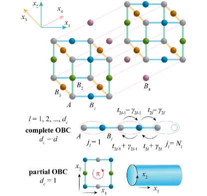
Figure 1: Lattice geometry of exactly solvable $d$-dimensional NH hypercubic models with OBCs in $d_{c}\leq d$ directions. In the presence of a magnetic field, the NH Lieb lattice with $\pi$ flux per plaquette becomes solvable by projecting to a cylinder.

Here, we pursue an alternative path to address the outstanding problem of the interplay between higher-dimensional NH skin and boundary modes. We present an extension of the GBZ approach in 1D to a class of NH hypercubic models, of which the exact solvability in arbitrary spatial dimensions and with arbitrary system sizes is associated with a spectral mirror symmetry. The OBC spectrum and the localization lengths related to NHSE belonging to all orders of skin modes can be resolved in the context of the GBZ that we here generalize to surface Brillouin zones. We test the Amoeba formulation in our models and clarify the topology of higher-order skin modes through the lens of biorthogonal polarization.

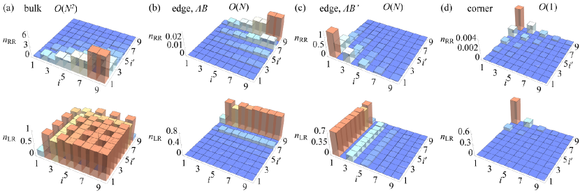
Figure 2: Total density comparison for the NH Lieb lattice: $n_{RR}$ vs $n_{LR}$. While $n_{RR}$ of the bulk (a), edge AB (b), edge AB’ (c) and corner (d) skin modes are centered towards different corners of the Lieb lattice, $n_{LR}$ shows whether the modes are of bulk, edge, or corner nature. $n_{LR}$ of the bulk modes becomes almost uniform (excluding holes, the empty sites on the Lieb lattice in Fig. 1). Summing over all types of skin modes, $n_{LR,\text{tot}}$ is normalized to $1$ on each available site. We take small size $N_{1,2}=5$ and choose hopping parameters $t_{1}=-1,t_{2}=2,\gamma_{1}=0.25,\gamma_{2}=0$ ($t_{3}=1,t_{4}=0.3,\gamma_{3}=0.5,\gamma_{4}=0$) along $x_{1}$ ($x_{2}$) direction denoted by site index $i$ ($i^{\prime}$).

Exact GBZ in higher dimensions.– As illustrated in Fig. 1, we build the NH Hamiltonian on a $d$-dimensional hypercubic lattice expanded by unit vectors $\vec{e}_{l}$: $\mathcal{H}=\sum_{\vec{j}}\sum_{l=1}^{d}t_{2l-1}^{+}c^{\dagger}_{\vec{j},A}c_{\vec{j},B_{l}}+t_{2l-1}^{-}c^{\dagger}_{\vec{j},B_{l}}c_{\vec{j},A}+t_{2l}^{+}c^{\dagger}_{\vec{j},B_{l}}c_{\vec{j}+\vec{e}_{l},A}+t_{2l}^{-}c^{\dagger}_{\vec{j}+\vec{e}_{l},A}c_{\vec{j},B_{l}}$, where $t^{\pm}_{l}=t_{l}\pm\gamma_{l}$. For simplicity, the hopping parameters $t_{l}$ and $\gamma_{l}$ are chosen to be real. $c^{\dagger}_{\vec{j},\lambda}$ ($c_{\vec{j},\lambda}$) creates (annihilates) a particle on the motif $\lambda\in\{A,B_{1},\dots,B_{d}\}$ inside the $j$-th unit cell with $\vec{j}=(j_{1},j_{2},\dots,j_{d})$. Along each direction $x_{l}$, the complete OBC leads to coupled arrays of odd-length NH SSH chains consisting of $N_{l}$ unit cells, each exactly solvable in 1D [45, 46]. We extend the exact solutions to higher dimensions. In the eigenvalue equations $H\ {\underline{\psi}}_{Rm}=E_{m}{\underline{\psi}}_{Rm},H^{\dagger}\ {\underline{\psi}}_{Lm}=E_{m}^{*}{\underline{\psi}}_{Lm}$, the left and right eigenvectors assigned with the band index $m$ respect biorthogonal relations [47]: ${\underline{\psi}}_{Lm}^{*}\cdot{\underline{\psi}}_{Rm^{\prime}}=\delta_{m,m^{\prime}}$. The notation $\underline{x}=(x_{1},x_{2},...,x_{k})^{T}$ is adopted to denote a vector of scalars or operators. Our real-space multi-band Hamiltonian corresponds to a multi-level block Toeplitz matrix [48]. After Fourier transform $c_{\vec{j},\lambda}=\frac{1}{\sqrt{N_{1}\dots N_{d}}}\sum_{\vec{k}}e^{i\vec{k}\cdot\vec{j}}c_{\vec{k},\lambda}$ with $k_{l}=\frac{2\pi\tilde{n}}{N_{l}}$ ($\tilde{n}=0,1,\dots,N_{l}-1$), its symbol becomes the Bloch Hamiltonian: $\mathcal{H}=\sum_{\vec{k}}\Psi_{\vec{k}}^{\dagger}H(\vec{k})\Psi_{\vec{k}}$, sharing the form in the basis $\Psi_{\vec{k}}=(c_{\vec{k},A},c_{\vec{k},B_{1}},\dots,c_{\vec{k},B_{d}})^{T}$:

$$H(k)=$$ (1)

$$\begin{pmatrix}0&t_{1}^{+}+t_{2}^{-}e^{-ik_{1}}&\dots&t_{2d-1}^{+}+t_{2d}^{-}e^{-ik_{d}}\\ t_{1}^{-}+t_{2}^{+}e^{ik_{1}}&0&&0\\ \vdots&&\ddots&\\ t_{2d-1}^{-}+t_{2d}^{+}e^{ik_{d}}&0&&0\end{pmatrix}$$

which exhibits two dispersive and $(d-1)$ zero-energy flat bands.

Although spectral mirror symmetry is not present with periodic boundary conditions (PBC), i.e. in the eigenvalues of Eq. 1, it is respected in every direction with OBCs:

$$E_{\alpha}^{\text{OBC}}(k_{l})=E_{\alpha}^{\text{OBC}}(-k_{l}),$$ (2)

where $\alpha=\pm,0$ and $k_{l}=\frac{\pi\tilde{m}}{N_{l}}\ (\tilde{m}=1,2,\dots,N_{l}-1)$. In analogy with 1D, the OBC and PBC spectra are related by an imaginary momentum shift [2, 23, 45, 46]: $k^{\prime}_{l}=k_{l}-i\ln r_{l}$. This characterizes GBZ by an unconventional Bloch phase factor $\beta_{l}=e^{ik^{\prime}_{l}}$ hosting a modulus $|\beta_{l}|=|r_{l}|\neq 1$ in general. In our model, we identify

$$r_{l}=\sqrt{\frac{r_{R,l}}{r^{*}_{L,l}}},\quad r_{R,l}=-\frac{t^{-}_{2l-1}}{t^{+}_{2l}},\quad r^{*}_{L,l}=-\frac{t^{+}_{2l-1}}{t^{-}_{2l}}.$$ (3)

The higher-order skin modes shown in Fig. 2 are obtained through a systematic dimension reduction [49] by identifying associated Bloch Hamiltonians as sub-blocks of $H(k)$ in Eq. 1. The one involving pairs $(t_{2l_{1}-1}^{\pm},t_{2l_{1}}^{\pm}),\dots,(t_{2l_{n}-1}^{\pm},t_{2l_{n}}^{\pm})$ generates a total number of ${\mathcal{O}(N^{n})}$ skin modes living on motifs $AB_{l_{1}}\cdots B_{l_{n}}$ with momentum $\vec{k}=(k_{l_{1}},\dots,k_{l_{n}},0,\dots,0)$. We take $n=0,1,\dots,d$, and for $n<d$, it refers to boundary modes. Our construction leads to the exact spectrum and the exact GBZ, which is extended to surface Brillouin zones, of right $\mathcal{O}(N^{n})$ skin modes [50]:

$$k_{l}\to(1-\delta_{k_{l},0})(k_{l}-i\ln r_{l})+\delta_{k_{l},0}(-i\ln r_{R,l}),$$ (4)

$$E_{n,\pm}^{\text{OBC}}(\vec{k})=E^{\text{PBC}}_{n,\pm}(k_{l}-i\ln r_{l})=\pm\sqrt{\sum_{l=l_{1}}^{l_{n}}g_{2l-1,2l}(k_{l})}.$$

Here, $r_{R,l}$ plays the role of cancelling the interference from neighbouring sites on unoccupied motifs, and the even $g$-functions read $g_{i,j}(q)=t_{i}^{+}t_{i}^{-}+t_{j}^{+}t_{j}^{-}+2\sqrt{t_{i}^{+}t_{j}^{+}}\sqrt{t_{i}^{-}t_{j}^{-}}\cos q$. Additionally, there exist $(n-1)$ zero-energy boundary (bulk) flat bands $E_{n,\ 0}^{\text{OBC}}(\vec{k})=0$ for $1<n<d\ (n=d)$. The GBZ approach also predicts the hybrid localization behaviour:

$$\underline{\psi}_{nR,(\alpha,\vec{k})}(\vec{j}) \propto\prod_{l\in\bar{l}_{n}}(r_{l})^{j_{l}}\prod_{l^{\prime}\notin\bar{l}_{n}}(r_{R,l^{\prime}})^{j_{l^{\prime}}},$$

$$\underline{\psi}_{nL,(\alpha,\vec{k})}(\vec{j}) \propto\prod_{l\in\bar{l}_{n}}(r^{*}_{l})^{-j_{l}}\prod_{l^{\prime}\notin\bar{l}_{n}}(r_{L,l^{\prime}})^{j_{l^{\prime}}},$$ (5)

with $\bar{l}_{n}=\{l_{1},\dots,l_{n}\}$. The dispersive part of the eigenvectors can be built as a superposition of non-Bloch waves at opposite momentum $\pm k_{l}$ [45, 46], fulfilling the requirement that its component vanishes at empty $B$ sites in last broken unit cells (see Fig. 1).

Let us consider 2D NH Lieb lattice as an example (see Fig. 2). Based on our exact solutions [50], Fig. 2 compares localization properties of different types of skin modes in terms of $n_{RR}(j)=\sum_{m}\langle\psi_{Rm}|\Pi_{j}|\psi_{Rm}\rangle$ and $n_{LR}(j)=\sum_{m}\langle\psi_{Lm}|\Pi_{j}|\psi_{Rm}\rangle$, with $\Pi_{j}=\sum_{\lambda}|\vec{j},\lambda\rangle\langle\vec{j},\lambda|$ and $|\vec{j},\lambda\rangle=c^{\dagger}_{\vec{j},\lambda}|0\rangle$. While in $n_{RR}$, all types of skin modes are centered at corners of the Lieb lattice under the influence of localization factors, the biorthogonal density $n_{LR}$ exhibits localization properties analogous to Hermitian systems and thereby motivates their categorization in terms of bulk, edge and corner modes.

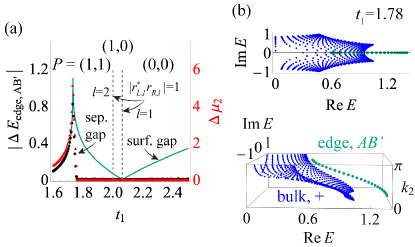
Figure 3: Gap comparison for the NH Lieb lattice: surface gap vs separation gap formed by the edge skin mode $AB^{\prime}$. While its surface gap with the bulk closes when biorthogonal polarization $P_{1}$ jumps at $|r^{*}_{L,1}r_{R,1}|=1$, its separation gap closing is accompanied by a vanishing Amoeba hole. In (a), we take size $N_{1,2}=26$ and choose a parameter path with $t_{1}=t_{3}$ and fixed $t_{2,4}=1$, $\gamma_{1,3}=\sqrt{3}$, $\gamma_{2}=1.5$, $\gamma_{4}=0$. (b) shows the distribution of energies of bulk ($+$) and edge $AB^{\prime}$ skin modes, displaying a closed separation gap (upper panel) and a finite surface gap (lower panel).

Biorthogonal polarization.– We proceed to locate topological phase transitions of higher-order edge skin modes through biorthorgonal polarization [3, 41]. It is built on the zero-energy corner skin mode, the associated right and left eigenvectors of which normalized by $\langle\underline{\psi}_{L0}|\underline{\psi}_{R0}\rangle=1$ live on the motif $A$ only: $E^{\text{OBC}}_{n=0}=0$,

$$|{\psi}_{R/L,0}\rangle=\mathcal{N}_{R/L}\sum_{\vec{j}}\prod_{l=1}^{d}(r_{R/L,l})^{j_{l}}c^{\dagger}_{\vec{j},A}|0\rangle.$$ (6)

The product encoding localization information can be viewed as a special case of Eq. 5 with $\bar{l_{0}}=\varnothing$. The polarization vector $\vec{P}=(P_{1},P_{2},\dots,P_{d})$ is quantized in the definition

$$P_{l}=1-\lim_{N_{l}\to\infty}\frac{1}{N_{l}}|\langle\psi_{L0}|\sum_{\vec{j}}j_{l}\Pi_{j}|\psi_{R0}\rangle|.$$ (7)

$P_{l}=1\ (0)$ when $|r^{*}_{L,l}r_{R,l}|<1\ (>1)$. In the non-Bloch band theory in presence of chiral symmetry, this polarization is equivalent to another topological invariant in GBZ, namely the winding number of edge skin modes [2]:

$$W_{l}=\frac{i}{2\pi}\int q_{l}^{-1}dq_{l},\quad|W_{l}|=P_{l},$$ (8)

with $q_{l}=-(t_{2l-1}^{+}+t_{2l}^{-}r_{l}^{-1}e^{-ik_{l}})/E_{AB_{l},+}^{\text{OBC}}(k_{l})$. In Fig. 3 (a) and Fig. 4 (a), we identify phase transitions of the second-order and third-order edge skin modes in 2D and 3D according to the value of $\vec{P}$ ($\vec{W}$) along selected parameter paths. As a diagnostic of bulk-boundary correspondence, the jump of $\vec{P}$ at $|r^{*}_{L,l}r_{R,l}|=1$ predicts surface gap closings between the bulk $O(N^{d})$ and higher-order $\mathcal{O}(N^{n})$ skin modes. It is convenient to introduce surface energy gap [51, 52]: $|\Delta E_{\text{Surf.}}(\vec{k}_{n})|=\min_{\forall\vec{q},\alpha,\alpha^{\prime}}\{|E_{d,\alpha}^{\text{OBC}}(\vec{k}_{n},\vec{q})-E^{\text{OBC}}_{n,\alpha^{\prime}}(\vec{k}_{n},\vec{0})|\}$ where $\vec{k}_{n}=(k_{l_{1}},\dots,k_{l_{n}})$ denotes the non-zero surface momentum of higher-order skin modes and $\alpha,\alpha^{\prime}\in\{\pm\}$. If $|\Delta E_{\text{Surf.}}|\neq 0$, the gap between their spectra and the bulk remains open at any surface momentum (see Fig. 3 (b), lower panel). It can be established that

$$\left.\Delta E_{\text{Surf.}}\right|_{N\to\infty}=0,\quad\text{if}\quad\Delta P_{\text{tot}}\neq 0.$$ (9)

From Fig. 4 (a), one further observes the total change in polarization $\Delta P_{\text{tot}}=\sum_{l}|\Delta P_{l}|$ imposes a constraint on the type of higher-order skin modes that can enter the bulk spectrum across the transition lines,

$$n\geq d-\Delta P_{\text{tot}}.$$ (10)

It results from the fact that $\Delta P_{\text{tot}}$ registers the number of zeros in the $g$-functions in Eq. 4: $g_{2l-1,2l}(\pi)=0$ at $r^{*}_{L,l}r_{R,l}=1$ and $g_{2l-1,2l}(0)=0$ at $r^{*}_{L,l}r_{R,l}=-1$.

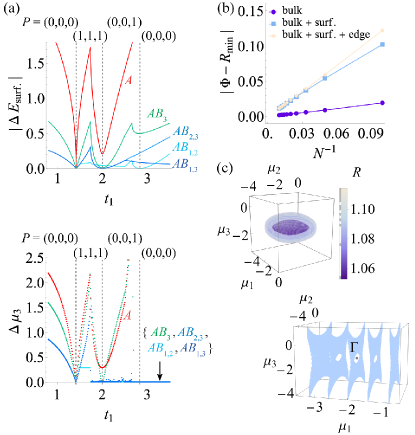
Figure 4: NH cubic lattice. (a) Surface gap vs Amoeba hole closings of $\mathcal{O}(N^{n})$ skin modes (marked by the motifs they occupy $AB_{l_{1},l_{2},\dots,l_{n}}$) across topological phase transition lines of edge skin modes. $\Delta P=3,2,1$ according to $|r^{*}_{L,l}r_{R,l}|=1$. Amoeba hole disappears at different places signaling separation gap closings. We choose $N_{1,2,3}=26$ and keep $t_{2,4,6}=1$, $\gamma_{1,3,5}=\sqrt{3}$, $\gamma_{2,4,6}=0$. The path varies with $t_{1}$: $t_{1}=t_{3,5}$ for $t_{1}\in[0.8,1.5]$; $t_{3}=t_{1},t_{5}=1.5$ for $t_{1}\in(1.5,2.5]$; $t_{3}=2.5,t_{5}=1.5t_{1}-2.25$ for $t_{1}\in(2.5,3.5]$; (b) Difference between Coulomb potential and Ronkin minimum as a function of system size $N=N_{1,2,3}$ at $E=0$, $t_{1}=0.8$. In $R_{\min}$, we take $\mu_{\min}=\mu_{c}$ and an integral grid with size $M_{1,2,3}=100$; (c) Illustration of 3D Amoeba hole in terms of Ronkin minimum and “vacuole” inside Amoeba body at $E=0,t_{1}=1.8$.

Amoeba formulation.– Next, we apply the Amoeba formulation [31] to locate the separation gap [51, 52] on the complex-energy plane: $|\Delta E_{\text{Sep.}}|=\min_{\forall\vec{k},\vec{k}^{\prime},\alpha,\alpha^{\prime}}\{|E_{d,\alpha}^{\text{OBC}}(\vec{k})-E^{\text{OBC}}_{n,\alpha^{\prime}}(\vec{k}^{\prime})|\}$. When $|\Delta E_{\text{Sep.}}|=0$, the spectra of $\mathcal{O}(N^{n})$ skin modes are inseparable from the bulk at normally different momenta [see Fig. 3 (b), upper panel]. The Amoeba is defined as a logarithmic map of solutions to the characteristic equation: $\mathcal{A}_{f}=\{\mu=\log|\beta|:f(\beta)=0\}$ where $f(\beta)=\det[H(\beta)-E]/E^{d-1}$. $H(\beta)$ denotes the Bloch Hamiltonian in Eq. 1 with $e^{ik_{l}}\to\beta_{l}$ and $E$ the reference energy. By dividing $E^{d-1}$, we neglect trivial solutions from $(d-1)$ zero-energy bulk flat bands. Notably, as observed from Fig. 3 (a), the separation gap closings are captured by an absence of hole inside Amoeba body [31]:

$$\left.\Delta E_{\text{Sep.}}\right|_{N\to\infty}=0,\quad\text{if}\quad\left.\mathcal{V}_{\text{hole}}\right|_{E=E^{\text{OBC}}_{n,\text{min}}}=0.$$ (11)

$\mathcal{V}_{\text{hole}}$ denotes the volume of Amoeba hole at the energy $E^{\text{OBC}}_{n,\text{min}}$ that minimizes the separation gap, with $\Delta\mu_{l}$ the longest distance it extends along the direction $x_{l}$. One can prove Eq. 11 in our models using the exact GBZ. Let us introduce the convex Ronkin function [39, 37, 38]: $R_{f}(\mu)=\int_{T^{d}}\frac{d^{d}q}{(2\pi)^{d}}\log|f(e^{\mu+iq})|$, which reaches its minimum in the Amoeba hole [see Fig. 4 (c)]. The exact GBZ predicts the center of the hole $\Gamma=\mu_{c}=(\log|r_{1}|,\log|r_{2}|,\dots,\log|r_{d}|)$. It can be verified [50] that $\partial_{\mu}R_{f}(\mu){\Large|}_{\mu=\mu_{c}}=0,\min_{\mu}R_{f}(\mu)=R_{f}(\mu_{c})$. Taking into account $\log|f(e^{\mu_{c}+iq})|=\sum_{\alpha=\pm}\log|E_{d,\alpha}^{\text{OBC}}(\vec{q})-E|$, when varying $E\notin E_{\text{bulk}}^{\text{OBC}}$, the Amoeba hole always encloses $\mu_{c}$ [$f(e^{\mu_{c}+iq})\neq 0$] and changes shape continuously in its vicinity. Once $E$ enters $E_{\text{bulk}}^{\text{OBC}}$, the hole closes at $\mu_{c}$.

We further compare in Fig. 4 (a) the analytical tools of polarization and Amoeba, and find the Amoeba fails to predict topological phase transitions of higher-order edge skin modes since the gaps they capture are intrinsically different: $\Delta E_{\text{Surf.}}\neq\Delta E_{\text{Sep.}}$. The two only match at boundary modes of codimension zero, e.g. the corner skin mode. Indeed, the jump of $\vec{P}$ is related to the Amoeba hole closing defined on edge Bloch Hamiltonians $f(\tilde{\beta}_{l})=\det[H_{\text{edge},AB_{l}}(\tilde{\beta}_{l})]$: $\Delta P_{l}=1,\Delta\tilde{\mu}_{l}=0$.

Finally, we address the influence of higher-order skin modes on the universal spectrum. Let us focus on the isolated spectrum in Fig. 4 (a) at small $t_{1}$ and compare its Coulomb potential with Ronkin function minimum [31]:

$$\Phi(E)=R_{\text{min}}+{\mathcal{O}(N^{-1})}.$$ (12)

Here, $\Phi(E)=\frac{1}{M}\sum_{m}\log|E_{m}-E|$ with a total number of $M$ eigenenergies $E_{m}$ selected from our exact solutions, determines the DOS through $\rho(E)=\frac{1}{2\pi}\Delta\Phi(E)$. While $\Phi(E)$ depends on the linear system size $N$, $R_{\text{min}}$ by definition is a universal quantity. Fig. 4 (b) indicates as $N$ increases, the convergence to the universal spectrum goes slower when the potential profile includes more types of boundary modes.

Discussion.– In this work we have exactly solved a class of NH models in any dimension. Our exact solutions make it explicit that no previously suggested approach is able to fully account for the interplay of bulk and boundary modes in these systems due to the presence of higher-dimensional NHSEs. However, we here successfully remedied these problems by combining and extending several previously distinct approaches. Specifically, we showed that the very recently proposed Amoeba theory [31] fully accounts for the $\mathcal{O}(N^{d})$ bulk modes. While the Amoeba approach does not account for any of the $\mathcal{O}(N^{d_{c}})$ boundary modes, we managed to fully describe those by generalizing the GBZ [2] and biorthogonal polarization [3] approaches to higher dimensions. While full analytical solvability of our models facilitates a direct confirmation of the aforementioned approaches, this is in general an exceedingly challenging task relying essentially on numerical tests. Some insights can however be obtained analytically by suitably extending the models described here. First of all, a prominent feature of our models is a generalized chiral symmetry. Insights can be gleaned from breaking chiral symmetry in one dimension where the GBZ winding numbers and the biorthogonal polarization still provide key information about phase transitions despite the winding number (but not the polarization) loosing its quantization [53, 54]. Our models are still solvable when distinct mass is added to each motif with broken chiral symmetry in every direction, and when $A$ motif includes internal degrees of freedom. Moreover, while we in the main text focused on complete OBC in all directions ($d_{c}=d$), the general case with hybrid boundary conditions $d_{c}<d$, can be accounted for analytically, as detailed in the supplementary material [50]. A concrete example comes from the cylinder geometry in Fig. 1, making it a convenient setting to study the effect of a magnetic field. At $\pi$ flux, with six sites in one unit cell, biorthogonal polarization and Amoeba formulation are generalized to capture four chiral edge skin modes. Here two zero-energy flat bands emerge reminiscent of the recently studied NH flat band topology in the quasi-1D diamond chain [55]. We also note that our models can be generalized to open quantum systems where the non-Hermiticity described by engineered Lindblad dissipators gives rise to the Liouvillian skin effect [56, 57, 46, 58, 59, 60, 61]. A dynamical distillation [62, 63, 64] of higher-order skin modes in the full master equation framework will be featured in a future work.

In conclusion, our present work marks a significant step towards a general quantitative understanding of the NHSE and its interplay with boundary modes in higher dimensions.

Appendix A Supplementary Material for “Anatomy of Higher-Order Non-Hermitian Skin and Boundary Modes”

In this supplementary material, we provide details on the derivation of the exact GBZ for the NH hybercubic models in arbitrary dimension $d$ with open boundaries in arbitrary $d_{c}\leq d$ directions. Exact solutions to the skin modes of all orders are presented for the NH Lieb lattice under the complete OBC. We also relate the GBZ approach to the Amoeba formulation through an analysis of the Ronkin function. In the end, we study one example of our models with hybrid boundaries, the NH Lieb model at $\pi$ flux on a cylinder. The interplay between four chiral edge skin modes and the bulk can be captured by generalized biorthogonal polarization and Amoeba formulation.

A.1 Exactly solvable NH hypercubic lattices

A.1.1 GBZ in arbitrary spatial dimension under complete OBC

To begin with, we give a proof of the existence of exact GBZ for the $\mathcal{O}(N^{n})$ skin modes in our NH hypercubic models under complete OBC ($d_{c}=d$) in Eq. 4 of the main text, which is one of the most important results in this work.

As a first step to diagonalize the multi-level block Toeplitz matrix, we generalize the method of the transformation matrix previously developed in 1D [2, 46], and map the original NH Hamiltonian to its effective Hermitian counterpart. Since it is more convenient to express the matrix algebra in the operator form, let us define a transformation matrix $S$ as a gauge transform on the annihilation operators,

$$\forall l:\quad c_{\vec{j},A}\to\prod_{i=1}^{d}(r_{i})^{j_{i}-1}\cdot c_{\vec{j},A},\quad c_{\vec{j},B_{l}}\to r_{l,1}\prod_{i=1}^{d}(r_{i})^{j_{i}-1}\cdot c_{\vec{j},B_{l}}.$$ (13)

The creation operators undergo the gauge transform simultaneously,

$$\forall l:\quad c^{\dagger}_{\vec{j},A}\to\prod_{i=1}^{d}(r_{i})^{-(j_{i}-1)}\cdot c^{\dagger}_{\vec{j},A},\quad c^{\dagger}_{\vec{j},B_{l}}\to r^{-1}_{l,1}\prod_{i=1}^{d}(r_{i})^{-(j_{i}-1)}\cdot c^{\dagger}_{\vec{j},B_{l}}.$$ (14)

We recall our NH lattice Hamiltonian with asymmetric real hopping amplitudes ($t_{l}^{\pm}=t_{l}\pm\gamma_{l}\in\mathbb{R}$),

$$\mathcal{H}=\sum_{\vec{j}}\sum_{l=1}^{d}t_{2l-1}^{+}c^{\dagger}_{\vec{j},A}c_{\vec{j},B_{l}}+t_{2l-1}^{-}c^{\dagger}_{\vec{j},B_{l}}c_{\vec{j},A}+t_{2l}^{+}c^{\dagger}_{\vec{j},B_{l}}c_{\vec{j}+\vec{e}_{l},A}+t_{2l}^{-}c^{\dagger}_{\vec{j}+\vec{e}_{l},A}c_{\vec{j},B_{l}}.$$ (15)

If we introduce a set of localization parameters into $S$,

$$r_{l,1}=\sqrt{\frac{t_{2l-1}^{-}}{t_{2l-1}^{+}}},\quad r_{l,2}=\sqrt{\frac{t_{2l}^{-}}{t_{2l}^{+}}},\quad r_{l}=r_{l,1}r_{l,2}=\sqrt{\frac{t_{2l-1}^{-}t_{2l}^{-}}{t_{2l-1}^{+}t_{2l}^{+}}},$$ (16)

after the transform, an effective Hermitian Hamiltonian arises

$$\tilde{\mathcal{H}}=S^{-1}\mathcal{H}S=\sum_{\vec{j}}\sum_{l=1}^{d}\tilde{t}_{2l-1}c^{\dagger}_{\vec{j},A}c_{\vec{j},B_{l}}+\tilde{t}_{2l}c^{\dagger}_{\vec{j},B_{l}}c_{\vec{j}+\vec{e}_{l},A}+\text{H.c.},$$ (17)

where

$$\tilde{t}_{l}=\sqrt{t_{l}^{+}t_{l}^{-}}.$$ (18)

Our goal is now simplified to diagonalize the Hermitian counterpart $\tilde{\mathcal{H}}$ in terms of $\mathcal{O}(N^{n})$ Hermitian bulk and boundary modes $|{\tilde{\psi}}_{n,m}\rangle$ assigned with band index $m$,

$$\tilde{\mathcal{H}}=\sum_{n}\sum_{m}\tilde{E}^{\text{OBC}}_{n,m}|{\tilde{\psi}}_{n,m}\rangle\langle{\tilde{\psi}}_{n,m}|.$$ (19)

Here, the summation over $n$ also includes all possible realizations of $\mathcal{O}(N^{n})$ eigenmodes that cover different motifs $AB_{l_{1}}\cdots B_{l_{n}}$ over the entire lattice. For convenience, we adopt the notation $\bar{l}_{n}=\{l_{1},\dots,l_{n}\}$. To achieve the decomposition in Eq. 19, we perform another gauge transform $U_{n}$, which projects the physical space from dimension $d$ to codimension $D=n$ in the limit $\epsilon\to 0^{+}$,

$$l\in\bar{l}_{n},\ l^{\prime}\notin\bar{l}_{n}:\quad c_{\vec{j},A}\to\prod_{i\notin\bar{l}_{n}}(\tilde{r}_{i})^{j_{i}}\cdot c_{\vec{j},A},\quad c_{\vec{j},B_{l}}\to\prod_{i\notin\bar{l}_{n}}(\tilde{r}_{i})^{j_{i}}\cdot c_{\vec{j},B_{l}},\quad c_{\vec{j},B_{l^{\prime}}}\to\epsilon\ c_{\vec{j},B_{l^{\prime}}},$$

$$c_{\vec{j},A}^{\dagger}\to\prod_{i\notin\bar{l}_{n}}(\tilde{r}_{i})^{-j_{i}}\cdot c^{\dagger}_{\vec{j},A},\quad c^{\dagger}_{\vec{j},B_{l}}\to\prod_{i\notin\bar{l}_{n}}(\tilde{r}_{i})^{-j_{i}}\cdot c^{\dagger}_{\vec{j},B_{l}},\quad c^{\dagger}_{\vec{j},B_{l^{\prime}}}\to\epsilon^{-1}\ c^{\dagger}_{\vec{j},B_{l^{\prime}}}.$$ (20)

Applying $U_{n}$ to $\tilde{H}$, one arrives at $U_{n}^{-1}\tilde{H}U_{n}=\tilde{H}_{n}+\tilde{H}^{\prime}_{n}$ with

$$\tilde{H}_{n}=\sum_{\vec{j}}\sum_{l\in\bar{l}_{n}}\tilde{t}_{2l-1}c^{\dagger}_{\vec{j},A}c_{\vec{j},B_{l}}+\tilde{t}_{2l}c^{\dagger}_{\vec{j},B_{l}}c_{\vec{j}+\vec{e}_{l},A}+\text{H.c.},$$ (21)

$$\left.\tilde{H}^{\prime}_{n}\right|_{\epsilon\to 0^{+}}=\sum_{\vec{j}}\sum_{l^{\prime}\notin\bar{l}_{n}}\epsilon^{-1}[\prod_{i\notin\bar{l}_{n}}(\tilde{r}_{i})^{j_{i}}](\tilde{t}_{2l^{\prime}-1}c^{\dagger}_{\vec{j},B_{l^{\prime}}}c_{\vec{j},A}+\tilde{t}_{2l^{\prime}}\cdot\tilde{r}_{l^{\prime}}c^{\dagger}_{\vec{j},B_{l^{\prime}}}c_{\vec{j}+\vec{e}_{l^{\prime}},A}).$$

When $\tilde{t}_{2l^{\prime}-1}+\tilde{t}_{2l^{\prime}}\cdot\tilde{r}_{l^{\prime}}=0$, the interference from neighbouring occupied $A$ sites on the unoccupied $B_{l^{\prime}}$ sites vanishes: $\tilde{H}^{\prime}_{n}\simeq 0$. Therefore, a second mapping is established in the physical limit $\epsilon\to 0^{+}$:

$$U_{n}^{-1}\tilde{H}U_{n}=\tilde{H}_{n},\quad\quad\text{for}\quad\tilde{r}_{l}=-\frac{\tilde{t}_{2l-1}}{\tilde{t}_{2l}}=-\sqrt{\frac{t_{2l-1}^{+}t_{2l-1}^{-}}{t_{2l}^{+}t_{2l}^{-}}}.$$ (22)

To obtain the exact OBC spectrum of $\tilde{\mathcal{H}}_{n}$, it is important to employ symmetries associated with different boundary conditions. Indicated by Fig. 1, for the hypercubic lattice under complete OBC, the last unit cells of which are broken in every direction, $\tilde{\mathcal{H}}_{n}$ inherits the spectral mirror symmetry: $\tilde{E}_{n,\alpha}^{\text{OBC}}(k_{l})=\tilde{E}_{n,\alpha}^{\text{OBC}}(-k_{l}),\forall l\in\bar{l}_{n}$. As a consequence, its OBC and PBC spectra coincide with each other: $\tilde{E}^{\text{OBC}}_{n,\alpha}(k)=\tilde{E}_{n,\alpha}^{\text{PBC}}(k)$. Here, $\alpha\in\{0,\pm\}$ comes from the generalized chiral symmetry of the Bloch Hamiltonian, in the representation $\mathcal{C}=\text{diag}\{1,-1,-1,\dots,-1\}$,

$$\tilde{H}_{n}(k)=\begin{pmatrix}0&\tilde{t}_{2l_{1}-1}+\tilde{t}_{2l_{1}}e^{-ik_{l_{1}}}&\dots&\tilde{t}_{2l_{n}-1}+\tilde{t}_{2l_{n}}e^{-ik_{l_{n}}}\\ \tilde{t}_{2l_{1}-1}+\tilde{t}_{2l_{1}}e^{ik_{l_{1}}}&0&&0\\ \vdots&&\ddots&\\ \tilde{t}_{2l_{n}-1}+\tilde{t}_{2l_{n}}e^{-ik_{l_{n}}}&0&&0\end{pmatrix},\quad\mathcal{C}\tilde{H}_{n}(k)\mathcal{C}^{-1}=-\tilde{H}_{n}(k).$$ (23)

Given $k$, apart from one pair of energies $\tilde{E}^{\text{PBC}}_{n,+}(k)=-\tilde{E}^{\text{PBC}}_{n,-}(k)$, there emerge $(n-1)$ zero-energy boundary (bulk) flat bands for $1<n<d$ ($n=d$): $\tilde{E}_{n,0}^{\text{PBC}}(k)=0$. From the second mapping in Eq. 20 and Eq. 22, one resolves the eigenvalue decomposition problem of the Hermitian Hamiltonian in Eq. 19:

$$\tilde{E}^{\text{OBC}}_{n,\alpha}(k)=\tilde{E}_{n,\alpha}^{\text{PBC}}(k),\quad|{\tilde{\psi}}_{n,\alpha}(k,j)\rangle\propto\prod_{i\notin\bar{l}_{n}}(\tilde{r}_{i})^{j_{i}}\cdot e^{ik\cdot j}|{\tilde{u}}_{n,\alpha}(k)\rangle,$$ (24)

where $|{\tilde{u}}_{n,\alpha}(k)\rangle$ denotes normalized eigenvectors of the Bloch Hamiltonian: $\tilde{H}_{n}(k)=\sum_{\alpha,k}\tilde{E}^{\text{PBC}}_{n,\alpha}(k)|{\tilde{u}}_{n,\alpha}(k)\rangle\langle{\tilde{u}}_{n,\alpha}(k)|$.

We are now ready to go back and derive the analytical solutions to the original NH Hamiltonian by taking the inverse of the first mapping in Eq. 17,

$$\mathcal{H}=S\tilde{\mathcal{H}}S^{-1}=\sum_{n}\sum_{\alpha,k}\tilde{E}^{\text{PBC}}_{n,\alpha}(k)S\tilde{P}_{n,\alpha}(k)S^{-1},\quad\tilde{P}_{n,\alpha}(k)=|{\tilde{\psi}}_{n,\alpha}(k)\rangle\langle{\tilde{\psi}}_{n,\alpha}(k)|.$$ (25)

Thanks to its Hermitian counterpart, the NH Hamiltonian is already decomposed in a formal form of $\mathcal{O}(N^{n})$ NH skin modes. The projection operator $\tilde{P}_{n,\alpha}(k)$ also enables us to focus on the subspace of occupied motifs where an effective basis $\underline{\psi}(j)=(c_{\vec{j},A},c_{\vec{j},B_{l_{1}}},\dots,c_{\vec{j},B_{l_{n}}})^{T}$ can be constructed for each unit cell. In this basis, the transformation matrix $S$ of Eq. 13 finds expression as

$$S\tilde{P}S^{-1}=S_{n}\tilde{P}S_{n}^{-1},\quad S_{n}=\bigoplus_{j}\prod_{i\in\bar{l}_{n}}(r_{i})^{j_{i}}\cdot S_{nj},\quad S_{nj}=\text{diag}\{1,r_{l_{1}},\dots,r_{{l_{n}}}\}\cdot\prod_{i\in\bar{l}_{n}}(r_{i})^{-1}.$$ (26)

It is straightforward to identify in Eq. 25 that in the $j$-th unit cell,

$$S_{nj}\tilde{H}_{n}(k)S_{nj}^{-1}=\begin{pmatrix}0&t_{2l_{1}-1}^{+}+t_{2l_{1}}^{-}r_{l_{1}}^{-1}e^{-ik_{l_{1}}}&\dots&t_{2l_{n}-1}^{+}+t_{2l_{n}}^{-}r_{l_{n}}^{-1}e^{-ik_{l_{n}}}\\ t_{2l_{1}-1}^{-}+t_{2l_{1}}^{+}r_{l_{1}}e^{ik_{l_{1}}}&0&&0\\ \vdots&&\ddots&\\ t_{2l_{n}-1}^{-}+t_{2l_{n}}^{+}r_{l_{n}}e^{ik_{l_{n}}}&0&&0\end{pmatrix}.$$ (27)

Comparing with the subblocks of the original NH Bloch Hamiltonian in Eq. 1 which act on motifs $AB_{l_{1}}\cdots B_{l_{n}}$, an equality can be established by a momentum shift:

$$S_{nj}\tilde{H}_{n}(\vec{k})S_{nj}^{-1}=H_{n}(k_{l}-i\ln r_{l}),\quad\forall l\in\bar{l}_{n}.$$ (28)

Taking into account ${H}_{n}(k)=\sum_{\alpha,k}{E}^{\text{PBC}}_{n,\alpha}(k)|{{u}}_{nR,\alpha}(k)\rangle\langle{{u}}_{nL,\alpha}(k)|$ in the biorthogonal basis $\langle{{u}}_{nL,\alpha}(k)|{{u}}_{nR,\alpha^{\prime}}(k)\rangle=\delta_{\alpha,\alpha^{\prime}}$, we obtain the eigenvalue decomposition of the NH Hamiltonian:

$$\mathcal{H}=\sum_{n}\sum_{\alpha,k}E_{n,\alpha}^{\text{OBC}}(k)|{\psi}_{nR,\alpha}(k)\rangle\langle{\psi}_{nL,\alpha}(k)|,$$

$$E_{n,\pm}^{\text{OBC}}(\vec{k})=E^{\text{PBC}}_{n,\pm}(k_{l}-i\ln r_{l}),\quad E_{n,0}^{\text{OBC}}(\vec{k})=0\ (n>1),$$ (29)

with the analytical functions,

$$E^{\text{PBC}}_{n,\pm}(\vec{k}) =\pm\sqrt{\sum_{l=l_{1}}^{l_{n}}f_{2l-1,2l}(k_{l})},\quad f_{i,j}(q)=t_{i}^{+}t_{i}^{-}+t_{j}^{+}t_{j}^{-}+2(t_{i}t_{j}+\gamma_{i}\gamma_{j})\cos q+2i(t_{i}\gamma_{j}+t_{j}\gamma_{i})\sin q,$$

$$E_{n,\pm}^{\text{OBC}}(\vec{k}) =\pm\sqrt{\sum_{l=l_{1}}^{l_{n}}g_{2l-1,2l}(k_{l})},\quad g_{i,j}(q)=t_{i}^{+}t_{i}^{-}+t_{j}^{+}t_{j}^{-}+2\sqrt{t_{i}^{+}t_{j}^{+}}\sqrt{t_{i}^{-}t_{j}^{-}}\cos q.$$ (30)

While the spectrum under OBC inherits the spectral mirror symmetry reflected in the even-$g$ functions, the PBC spectrum is not invariant under $k_{l}\to-k_{l}$. From Eqs. (24)-(26), the left and right $\mathcal{O}(N^{n})$ skin modes exhibit hybrid localization behaviours:

$$|{\psi}_{nR,(\alpha,k)}(\vec{j})\rangle\propto\prod_{l\in\bar{l}_{n}}(r_{l})^{j_{l}}\prod_{l^{\prime}\notin\bar{l}_{n}}(r_{R,l^{\prime}})^{j_{l^{\prime}}}\cdot e^{ik\cdot j}|{u}_{nR,\alpha}(k_{l}-i\ln r_{l})\rangle,$$

$$\langle{\psi}_{nL,(\alpha,k)}(\vec{j})|\propto\prod_{l\in\bar{l}_{n}}(r_{l})^{-j_{l}}\prod_{l^{\prime}\notin\bar{l}_{n}}(r^{*}_{L,l^{\prime}})^{j_{l^{\prime}}}\cdot e^{ik\cdot j}\langle{u}_{nL,\alpha}(k_{l}-i\ln r_{l})|,$$ (31)

where the localization parameters read

$$r_{R,l}=r_{l}\tilde{r}_{l}=-\frac{t^{-}_{2l-1}}{t^{+}_{2l}},\quad r^{*}_{L,l}=r^{-1}_{l}\tilde{r}_{l}=-\frac{t^{+}_{2l-1}}{t^{-}_{2l}}.$$ (32)

Eq. 31 can also be obtained by performing imaginary momentum shifts on $\vec{k}=(k_{l_{1}},\dots,k_{l_{n}},0,\dots,0)$, which leads to the exact GBZ for the right $\mathcal{O}(N^{n})$ skin modes:

$$k_{l}\to(1-\delta_{k_{l},0})(k_{l}-i\ln r_{l})+\delta_{k_{l},0}(-i\ln r_{R,l}).$$ (33)

The exact skin modes can be further built from Eq. 31 by taking a superposition of non-Bloch waves at opposite momenta $\pm k_{l}$, such that the total wavefunction meets the boundary condition with vanishing component on the empty $B_{l}$ sites of last broken unit cells (see Fig. 1). It is also interesting to comment on the structures of biorthogonal eigenvectors $|u_{nR/L}\rangle$ associated with the non-Bloch Hamiltonian in Eq. 27. It can be checked that while the eigenvectors of the two dispersive bands in Eq. 29 live on all $AB_{l_{1}}\cdots B_{l_{n}}$ motifs, the ones for those flat bands have zero occupancy on the $A$ motif. And by satisfying one more condition from the eigenvalue equation, they can be built as $(n-1)$ linearly independent states covering all $B_{l_{1}}\cdots B_{l_{n}}$ motifs, thus fulfilling the requirement of a codimension $D=n$.

Meanwhile, with gauge transforms, we are able to retrieve the phase transitions of higher-order edge skin modes in our models. It immediately follows from Eq. 17 that on motifs $AB_{l}$, the complex gap of the edge skin mode closes as soon as its Hermitian counterpart $\tilde{\mathcal{H}}_{AB_{l}}=\sum_{\vec{j}}\tilde{t}_{2l-1}c^{\dagger}_{\vec{j},A}c_{\vec{j},B_{l}}+\tilde{t}_{2l}c^{\dagger}_{\vec{j},B_{l}}c_{\vec{j}+\vec{e}_{l},A}+\text{H.c.}$ becomes gapless:

$$|\tilde{t}_{2l-1}|=|\tilde{t}_{2l}|\quad\Longleftrightarrow\quad|r^{*}_{L,l}r_{R,l}|=1.$$ (34)

From the biorthogonal bulk-boundary correspondence, these gapless lines are accompanied by a quantized change in topological invariants in NH systems compatible with open boundaries: the biorthogonal polarization of the corner skin mode or the GBZ winding number of the edge skin modes in presence of chiral symmetry [see Eq. 7 and Eq. 8 of the main text].

A.1.2 GBZ for boundaries of arbitrary codimension

Next, we address our NH hypercubic models under hybrid boundary conditions ($d_{c}<d$): $\text{OBC}_{d_{c}}+\text{PBC}_{d-d_{c}}$.

In the spatial dimension $d$ with open boundary conditions in $d_{c}$ directions and periodic boundary conditions in $d-d_{c}$ directions, it yields boundary skin modes of codimension $D=0,1,\ldots,d_{c}-1$, the total number of which is proportional to $\mathcal{O}(N^{n})$ with $n=d-d_{c}+D$ or $n=d-d_{c},\dots,d-1$. For bulk skin modes, $D=d_{c}$, $n=d$. To further simplify notations, we adopt symbols $\perp$ and $\parallel$ to denote elements in the OBC and PBC directions. In this manner, the spectral mirror symmetry related to momenta along the OBC directions, is manifested as $E(k_{\perp},k_{\parallel})=E(-k_{\perp},k_{\parallel})$.

In the full NH lattice Hamiltonian $\mathcal{H}=\mathcal{H}_{\perp}+\mathcal{H}_{\parallel}$, it is convenient to first diagonalize $\mathcal{H}_{\parallel}$ and create a new $\tilde{A}$ motif from its eigenmodes, such that the original $A$ motif and the $B_{\perp}$ motifs are all absorbed into the $\tilde{A}$ motif as $(d-d_{c}+1)$ internal degrees of freedom. To acheive this, we perform the Fourier transform along the PBC directions on the operators,

$$c_{j_{\perp},\lambda}(j_{\parallel})=\frac{1}{\sqrt{\prod_{l\in\bar{l}_{\parallel}}N_{l}}}\sum_{k_{\parallel}}e^{ik_{\parallel}\cdot j_{\parallel}}c_{j_{\perp},\lambda}(k_{\parallel}),$$ (35)

where $\lambda\in\{A,B_{1},\cdots B_{d}\}=A\cup B_{\perp}\cup B_{\parallel}$ with ${B}_{\perp}=\{B_{1},\cdots B_{d}\}-B_{\parallel}$, $B_{\parallel}=\{B_{m_{1}},\cdots B_{m_{d-d_{c}}}\}$, and $k_{\parallel,l}=\frac{2\pi\tilde{n}}{N_{l}}$ ($\tilde{n}=0,1,\dots,N_{l}-1$) for $l\in\bar{l}_{\parallel}=\{m_{1},\dots,m_{d-d_{c}}\}$. The subscript $j_{\perp}$ can be ignored for the moment. Given each $k_{\parallel}$, in the basis $\underline{\varphi}(k_{\parallel})=(c_{A}(k_{\parallel}),c_{B_{\parallel}}(k_{\parallel}))^{T}$, the Bloch Hamiltonian of $\mathcal{H}_{\parallel}$ shares the form

$$H_{\parallel}(k_{\parallel})=\begin{pmatrix}0&t_{2m_{1}-1}^{+}+t_{2m_{1}}^{-}e^{-ik_{m_{1}}}&\dots&t_{2m_{d-d_{c}}-1}^{+}+t_{2m_{d-d_{c}}}^{-}e^{-ik_{m_{d-d_{c}}}}\\ t_{2m_{1}-1}^{-}+t_{2m_{1}}^{+}e^{ik_{m_{1}}}&0&&0\\ \vdots&&\ddots&\\ t_{2m_{d-d_{c}}-1}^{-}+t_{2m_{d-d_{c}}}^{+}e^{ik_{m_{d-d_{c}}}}&0&&0\end{pmatrix}.$$ (36)

After the diagonalization, there emerge two dispersive bands and $(d-d_{c}-1)$ zero-energy flat bands:

$$H_{\parallel}(k_{\parallel})=\sum_{\alpha}\epsilon_{\tilde{A},\alpha}(k_{\parallel})|\varphi_{R,\alpha}(k_{\parallel})\rangle\langle\varphi_{L,\alpha}(k_{\parallel})|,$$

$$\quad\epsilon_{\tilde{A},\pm}(k_{\parallel})=\pm\sqrt{\sum_{l\in\bar{l}_{\parallel}}f_{2l-1,2l}(k_{\parallel})},\quad\epsilon_{\tilde{A},0}(k_{\parallel})=0\ (d-d_{c}>1),$$ (37)

with the $f$-functions given by Eq. 30. Identifying each eigenmode of $H_{\parallel}(k_{\parallel})$ as a particle on the new $\tilde{A}$ motif,

$$|\varphi_{R,i}(k_{\parallel})\rangle=c_{\tilde{A}_{i}}^{\dagger}(k_{\parallel})|0\rangle,\quad\langle\varphi_{L,i}(k_{\parallel})|=\langle 0|c_{\tilde{A}_{i}}(k_{\parallel}),$$ (38)

we arrive at

$$H_{\parallel}(k_{\parallel})=\sum_{i=1}^{d-d_{c}+1}\epsilon_{\tilde{A}_{i}}(k_{\parallel})c_{\tilde{A}_{i}}^{\dagger}(k_{\parallel})c_{\tilde{A}_{i}}(k_{\parallel}).$$ (39)

It is interesting to see the coexistence of non-skin modes and skin modes under hybrid boundary conditions. Particles on the $\tilde{A}$ motifs are coupled to the $B_{\perp}$ motifs through the original $A$ sites,

$$c_{A}^{\dagger}(k_{\parallel})=\sum_{i}\varphi_{L,i}^{*}(k_{\parallel},1)c_{\tilde{A}_{i}}^{\dagger}(k_{\parallel}),\quad c_{A}(k_{\parallel})=\sum_{i}\varphi_{R,i}(k_{\parallel},1)c_{\tilde{A}_{i}}(k_{\parallel}),$$ (40)

where we have applied to Eq. 38 $|\varphi_{R/L,i}(k_{\parallel})\rangle=\sum_{\lambda\in A\cup B_{\parallel}}\varphi_{R/L,i}(k_{\parallel},\lambda)c_{\lambda}^{\dagger}(k_{\parallel})|0\rangle$ and the identity $\mathbbm{1}_{\lambda}=\sum_{i}|\varphi_{R,i}(k_{\parallel},\lambda)\rangle\langle\varphi_{L,i}(k_{\parallel},\lambda)|$. Taking into account the zero-energy eigenmodes of PBC flat bands in Eq. 37 vanish on the $A$ motif: $\varphi_{L,\alpha=0}^{*}(k_{\parallel},1)=\varphi_{R,\alpha=0}(k_{\parallel},1)=0$, they constitute $(d-d_{c}-1)$ non-skin (non-localized) modes living exclusively on the $B_{\parallel}$ motifs that can be described by the normal BZ along the PBC directions. On the other hand, the two eigenmodes with opposite energies $(\alpha=\pm)$ belonging to the PBC dispersive bands are elevated to localized skin modes when NHSEs along OBC directions come into play.

Restoring the unit cell index $j_{\perp}$ in Eq. 35, one builds on the effective $\tilde{A}B_{\perp}$ motifs a generalized NH hypercubic model under complete OBC: $\mathcal{H}=\sum_{k_{\parallel}}\mathcal{H}(k_{\parallel})$,

$$\mathcal{H}(k_{\parallel})=\sum_{\alpha=\pm}\sum_{\vec{j}_{\perp}}\sum_{l\in\bar{l}_{\perp}} \epsilon_{\tilde{A},\alpha}(k_{\parallel})c_{\vec{j}_{\perp},\tilde{A}_{\alpha}}^{\dagger}(k_{\parallel})c_{\vec{j}_{\perp},\tilde{A}_{\alpha}}(k_{\parallel})+{t}_{2l-1,\alpha}^{+}c^{\dagger}_{\vec{j}_{\perp},\tilde{A}_{\alpha}}(k_{\parallel})c_{\vec{j}_{\perp},B_{l}}(k_{\parallel})+t_{2l-1,\alpha}^{-}c^{\dagger}_{\vec{j}_{\perp},B_{l}}(k_{\parallel})c_{\vec{j}_{\perp},\tilde{A}_{\alpha}}(k_{\parallel})$$

$$+t_{2l,\alpha}^{+}c^{\dagger}_{\vec{j}_{\perp},B_{l}}(k_{\parallel})c_{\vec{j}_{\perp}+\vec{e}_{l},\tilde{A}_{\alpha}}(k_{\parallel})+t_{2l,\alpha}^{-}c^{\dagger}_{\vec{j}_{\perp}+\vec{e}_{l},\tilde{A}_{\alpha}}(k_{\parallel})c_{\vec{j}_{\perp},B_{l}}(k_{\parallel}),$$ (41)

with renormalized asymmetric hopping parameters from Eq. 40,

$$t_{2l-1,\alpha}^{+}=t_{2l-1}^{+}\varphi_{L,\alpha}^{*}(k_{\parallel},1),\quad t_{2l-1,\alpha}^{-}=t_{2l-1}^{-}\varphi_{R,\alpha}(k_{\parallel},1),\quad t_{2l,\alpha}^{+}=t_{2l}^{+}\varphi_{R,\alpha}(k_{\parallel},1),\quad t_{2l,\alpha}^{-}=t_{2l}^{-}\varphi^{*}_{L,\alpha}(k_{\parallel},1).$$ (42)

Although the effective mass term $\epsilon_{\tilde{A},\alpha}(k_{\parallel})\neq 0$ breaks generalized chiral symmetry, the solvability of our models remains unaffected since spectral mirror symmetry is still respected along the OBC directions $E(k_{\perp},k_{\parallel})=E(-k_{\perp},k_{\parallel})$, and equally important, the same localization parameter $r_{l}^{\alpha}$ is shared by two independent particles on the $\tilde{A}$ motif:

$$r_{R,l}^{\alpha}=-\frac{t_{2l-1,\alpha}^{-}}{t_{2l,\alpha}^{+}}=-\frac{t_{2l-1}^{-}}{t_{2l}^{+}}=r_{R,l},\quad r_{L,l}^{\alpha*}=-\frac{t_{2l-1,\alpha}^{+}}{t_{2l,\alpha}^{-}}=-\frac{t_{2l-1}^{+}}{t_{2l}^{-}}=r_{L,l},$$

$$r_{l}^{\alpha}=\sqrt{\frac{r_{R,l}^{\alpha}}{r_{L,l}^{\alpha*}}}=\sqrt{\frac{t_{2l-1}^{-}t_{2l}^{-}}{t_{2l-1}^{+}t_{2l}^{+}}}=r_{l}.$$ (43)

As a consequence, the two exact mappings $S$ and $U$ for the Hamiltonian $\mathcal{H}(k_{\parallel})$ in Eq. 41 under complete OBC can be established by simply replacing in Eqs. (13)-(14) and Eq. 20:

$$\bar{l}_{d}\to\bar{l}_{\perp},\quad\bar{l}_{n}\to\bar{l}_{D},\quad c_{\vec{j},\lambda}\to c_{\vec{j}_{\perp},\lambda}(k_{\parallel}),$$ (44)

where $\bar{l}_{d}=\bar{l}_{\perp}\cup\bar{l}_{\parallel}$, and $\bar{l}_{D}=\{l_{1},\dots,l_{D}\}\in\bar{l}_{\perp}$ denotes the motifs $\tilde{A}_{\alpha}B_{l_{1}}\cdots B_{l_{D}}$ covered by the ${\mathcal{O}(N^{n})}$ skin modes of codimension $D=0,1,\dots,d_{c}$ with $n=d-d_{c}+D$. The extra $(d-d_{c})$ arises from the degrees of freedom in PBC dimensions encoded in each $\tilde{A}_{\alpha}$ particle in Eq. 38. Moreover, the solvability can be further relaxed to different values of $r_{R/L,l}^{\alpha}$, which corresponds to different localization factors $\tilde{r}_{l}^{\alpha}=r^{\alpha}_{R,l}/r_{l}$ in $U$, as the contributions from the occupied $\tilde{A}_{\alpha}$ sites on the unoccupied $B_{\perp}$ motifs can be cancelled independently (see the example of the cylinder geometry at $\pi$ flux). However, the transformation matrix $S$ acts on the common $B_{\perp}$ motifs, leading to a unique $r_{l}$ factor.

Performing the Fourier transform along the OBC directions on the Hamiltonian $\mathcal{H}(k_{\parallel})$ of Eq. 41,

$$c_{j_{\perp},\lambda}(k_{\parallel})=\frac{1}{\sqrt{\prod_{l\in\bar{l}_{\perp}}N_{l}}}\sum_{k_{\perp}}e^{ik_{\perp}\cdot j_{\perp}}c_{\lambda}(k_{\perp},k_{\parallel}),$$ (45)

with $\lambda\in\tilde{A}\cup B_{\perp}$, followed by imaginary momentum shifts in the GBZ, we can obtain the non-Bloch Hamiltonian for the ${\mathcal{O}(N^{n})}$ skin modes of codimension $D=0,1,\dots,d_{c}$. As the eigen energies do not change with a different biorthogonal basis, we can either stay with the new basis $\tilde{A}\cup B_{\perp}^{D}$ or choose the original basis with motifs $A\cup B_{\parallel}\cup B_{\perp}^{D}$, where $B_{\perp}^{D}=\{B_{l_{1}},\dots,B_{l_{D}}\}$. It turns out that while the former is convenient for identifying corner skin modes, the latter is a more natural choice to get access to the skin modes of codimension $D>0$. In the original basis $\underline{\psi}(k_{\perp},k_{\parallel})=(c_{A}(k_{\perp},k_{\parallel}),c_{B_{\parallel}}(k_{\perp},k_{\parallel}),c_{B_{\perp}^{D}}(k_{\perp},k_{\parallel}))^{T}$, the non-Bloch Hamiltonian for $O(N^{n})$ skin modes has the structure

$$H_{D}(k_{l}-i\ln r_{l},k_{\parallel})=\begin{pmatrix}0&H_{\parallel,-}&H_{\perp,-}\\ H_{\parallel,+}^{T}&0&0\\ H_{\perp,+}^{T}&0&0\end{pmatrix},$$ (46)

with the matrix elements

$$H_{\parallel,\pm} =(t_{2m_{1}-1}^{\mp}+t_{2m_{1}}^{\pm}e^{\pm ik_{m_{1}}},\ \dots,\ t_{2m_{d-d_{c}}-1}^{\mp}+t_{2m_{d-d_{c}}}^{\pm}e^{\pm ik_{m_{d-d_{c}}}}),$$

$$H_{\perp,\pm} =(t_{2l_{1}-1}^{\mp}+t_{2l_{1}}^{\pm}(r_{l_{1}})^{\pm 1}e^{\pm ik_{l_{1}}},\ \dots,\ t_{2l_{D}-1}^{\mp}+t_{2l_{D}}^{\pm}(r_{l_{D}})^{\pm 1}e^{\pm ik_{l_{D}}}).$$ (47)

The exact spectrum follows

$$E_{D,\pm}^{\text{OBC}}(\vec{k})=\pm\sqrt{\sum_{l\in\bar{l}_{\parallel}}f_{2l-1,2l}(k_{l})+\sum_{l\in\bar{l}_{D}}g_{2l-1,2l}(k_{l})},\quad E_{D,0}(\vec{k})=0\ (D>0),$$ (48)

where $f$ and $g$-functions are given in Eq. 30. There are two corner skin modes of codimension $D=0$ at $\bar{l}_{D}=\varnothing$ endowed with opposite energies $\epsilon_{\tilde{A},\pm}(k_{\parallel})$ in Eq. 37, and they are localized on the $\tilde{A}_{+}$ and $\tilde{A}_{-}$ motifs. By taking $\bar{l}_{\parallel}=\varnothing$, the two dispersive bands under hybrid boundary conditions ($d_{c}<d$) are connected to those under the complete OBC ($d_{c}=d$) in Eq. 30. At the same time, in addition to $(d-d_{c}-1)$ zero-energy bulk flat bands in normal BZ along the PBCs in Eq. 37 accounting for non-localized modes that cover only the $B_{\parallel}$ motifs, there exist $D$ zero-energy boundary (bulk) flat bands in GBZ as well for $1\leq D<d_{c}\ (D=d_{c})$ accounting for the skin modes that are exponentially localized (delocalized) on the $B_{\perp}$ ($B_{\parallel}$) motifs and vanish completely on the $A$ motif. In this way, we retrieve in total $n=2+d-d_{c}-1+D=d-d_{c}+D$ bands for the $O(N^{n})$ skin modes.

Under hybrid boundary conditions, given the surface momentum $\vec{k}=(k_{\perp},k_{\parallel})=(k_{l_{1}},\dots,k_{l_{D}},0,\dots,0;k_{\parallel})$, the exact GBZ for the right ${\mathcal{O}(N^{n})}$ skin modes is generalized to

$$\forall l\in\bar{l}_{\perp}:k_{l}\to(1-\delta_{k_{l},0})(k_{l}-i\ln r_{l})+\delta_{k_{l},0}(-i\ln r_{R,l}),$$ (49)

which is consistent with hybrid localization behaviours in the exact mappings $(\alpha=\pm,0)$,

$$|{\psi}_{D,R,(\alpha,k)}(\vec{j})\rangle\propto\prod_{l\in\bar{l}_{D}}(r_{l})^{j_{\perp,l}}\prod_{l^{\prime}\in(\bar{l}_{\perp}-\bar{l}_{D})}(r_{R,l^{\prime}})^{j_{\perp,l^{\prime}}}\cdot e^{i\vec{k}\cdot\vec{j}}|{u}_{D,R,\alpha}(k_{l}-i\ln r_{l},k_{\parallel})\rangle,$$

$$\langle{\psi}_{D,L,(\alpha,\vec{k})}(\vec{j})|\propto\prod_{l\in\bar{l}_{D}}(r_{l})^{-j_{\perp,l}}\prod_{l^{\prime}\in(\bar{l}_{\perp}-\bar{l}_{D})}(r_{L,l^{\prime}}^{*})^{j_{\perp,l^{\prime}}}\cdot e^{i\vec{k}\cdot\vec{j}}\langle{u}_{D,L,\alpha}(k_{l}-i\ln r_{l},k_{\parallel})|,$$ (50)

where $|u_{D,R/L,\alpha}\rangle$ represent the biorthogonal eigenvectors of the non-Bloch Hamiltonian in Eq. 46.

In the end, we comment briefly on the analytical tools that can be developed to detect the gap closings in our models with hybrid boundaries. In absence of chiral symmetry in the non-Bloch Hamiltonian of Eq. 46, the GBZ winding number is no longer a good invariant. In order to capture the surface gap closings of the higher-order skin modes, one can extend the more robust biorthogonal polarization to include two corner skin modes,

$$|{\psi}_{R/L,0,\alpha=\pm}(k_{\parallel})\rangle=\mathcal{N}_{R/L,\alpha}(k_{\parallel})\sum_{\vec{j}_{\perp}}\prod_{l\in\bar{l}_{\perp}}(r_{R/L,l})^{j_{\perp,l}}c^{\dagger}_{\vec{j}_{\perp},\tilde{A}_{\alpha}}(k_{\parallel})|0\rangle.$$ (51)

We define the generalized polarization vector $\vec{P}$ with

$$l\in\bar{l}_{\perp},\quad P_{l}=2-\lim_{N_{l}\to\infty}\frac{1}{N_{l}}\sum_{\alpha=\pm}|\langle\psi_{L0,\alpha}(k_{\parallel})|\sum_{\vec{j}_{\perp}}j_{\perp,l}\Pi_{j_{\perp}}(k_{\parallel})|\psi_{R0,\alpha}(k_{\parallel})\rangle|.$$ (52)

Here, $\Pi_{j_{\perp}}(k_{\parallel})=\sum_{\lambda\in\tilde{A}}|\vec{j}_{\perp},\lambda,k_{\parallel}\rangle\langle\vec{j}_{\perp},\lambda,k_{\parallel}|$ and $|\vec{j},\lambda,k_{\parallel}\rangle=c^{\dagger}_{\vec{j}_{\perp},\lambda}(k_{\parallel})|0\rangle$. Since the localization factors of two corner skin modes do not depend on $k_{\parallel}$ and $\langle{\psi}_{L0,\alpha}(k_{\parallel})|{\psi}_{R0,\alpha}(k_{\parallel})\rangle=1$, $P_{l}$ does not vary with $k_{\parallel}$. $P_{l}=2\ (0)$ when $|r^{*}_{L,l}r_{R,l}|<1\ (>1)$. In a similar manner, the separation gaps with the bulk skin modes on the motifs $AB_{\parallel}B_{\perp}$ can be captured by the generalized Amoeba of codimension $d_{c}$ as a function of $k_{\parallel}$: $\mathcal{A}_{f}(k_{\parallel})=\{\mu(k_{\parallel})=\log|\beta(k_{\parallel})|:f(\beta)=0\}$ where $f(\beta)=\det[H(\beta,k_{\parallel})-E]/E^{d-1}$ and $E$ denotes the reference energy. The trivial solutions from $(d-1)$ zero-energy bulk flat bands are excluded by the denominator. By analogy to the complete OBC, here $H(\beta,k_{\parallel})$ comes from the bulk Bloch Hamiltonian with $\beta_{l}=e^{ik_{l}}$ for any $l\in\bar{l}_{\perp}=\{l_{1},\dots,l_{d_{c}}\}$ along the OBC directions,

$$H(\beta,k_{\parallel})=\begin{pmatrix}0&H_{\parallel,-}(k_{\parallel})&H_{\perp,-}(\beta)\\ H_{\parallel,+}^{T}(k_{\parallel})&0&0\\ H_{\perp,+}^{T}(\beta)&0&0\end{pmatrix},\quad H_{\perp,\pm}(\beta)=(t_{2l_{1}-1}^{\mp}+t_{2l_{1}}^{\pm}\beta_{l_{1}}^{\pm},\ \dots,\ t_{2l_{d_{c}}-1}^{\mp}+t_{2l_{d_{c}}}^{\pm}\beta_{l_{d_{c}}}^{\pm}).$$ (53)

A.1.3 Exact solutions to the NH Lieb lattice under complete OBC

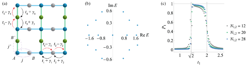
Figure 5: (a) Lattice geometry of the NH Lieb lattice; (b) Comparison of complex eigenvalues between the numerical (dark blue) and analytical (light blue) results for a finite-size Lieb lattice with $N_{1,2}=3$. We choose distinct values for all hopping parameters: $\{t_{1},t_{2},t_{3},t_{4}\}=\{1.5,1,1.6,1.2\}$, $\{\gamma_{1},\gamma_{2},\gamma_{3},\gamma_{4}\}=\{\sqrt{3},0.2,\sqrt{2},0.4\}$; (c) Quantization of polarization $P_{1}$ with varying system size as a function of $t_{1}$. We keep $t_{1}=t_{3}$ and fix $t_{2,4}=1,\gamma_{1,3}=\sqrt{3},\gamma_{2,4}=0$. $P_{1}$ jumps at $|r^{*}_{L,1}r_{R,1}|=1$.

In this section, we give an explicit example of the diverse types of skin modes in our NH hypercubic models in 2D, the NH Lieb lattice. Starting from the results of the exact mappings in Eq. 31, we finalize the construction of eigenmodes by taking into account spectral mirror symmetry and boundary constraints under complete OBC.

Fig. 5 (a) illustrates the geometry of the NH Lieb lattice of size $(2N_{1}-1)\times(2N_{2}-1)$ where we designate three motifs $ABB^{\prime}$ in each unit cell at the position $\vec{j}=(j,j^{\prime})$ with $j=1,\dots,N_{1}$ and $j^{\prime}=1,\dots,N_{2}$. There are $N_{\text{tot}}=3N_{1}N_{2}-N_{1}-N_{2}$ sites, equal to the total number of $\mathcal{O}(N^{n})$ skin modes ($n=0,1,2$). Among them, we recognize one corner skin mode at $k_{0}=(0,0)$, $2(N_{1}-1)+2(N_{2}-1)$ edge skin modes at $k_{\text{edge}}=(k_{1},0),(0,k_{2})$ and $3(N_{1}-1)(N_{2}-1)$ bulk skin modes at $k_{\text{bulk}}=(k_{1},k_{2})$. They correspond to the third-order, second-order and first-order NHSEs in two dimensions. Let us first test the exact spectrum in Eq. 29 related to imaginary momentum shifts in the GBZ,

$${\mathcal{O}(1)}:\quad E^{\text{OBC}}_{\text{corner}}(0,0)=0,$$

$${\mathcal{O}(N)}:\quad E^{\text{OBC}}_{\text{edge},AB,\pm}(k_{1},0)=E^{\text{PBC}}_{\text{edge},AB,\pm}(k_{1}-i\ln r_{1})=\pm\sqrt{g_{1,2}(k_{1})},$$

$$E^{\text{OBC}}_{\text{edge},AB^{\prime},\pm}(0,k_{2})=E^{\text{PBC}}_{\text{edge},AB^{\prime},\pm}(k_{2}-i\ln r_{2})=\pm\sqrt{g_{3,4}(k_{2})},$$

$${\mathcal{O}(N^{2})}:\quad E^{\text{OBC}}_{\text{bulk},0}(k_{1},k_{2})=0,$$

$$E^{\text{OBC}}_{\text{bulk},\pm}(k_{1},k_{2})=E^{\text{PBC}}_{\text{bulk},\pm}(k_{1}-i\ln r_{1},k_{2}-i\ln r_{2})=\pm\sqrt{g_{1,2}(k_{1})+g_{3,4}(k_{2})},$$ (54)

with

$$r_{1}=\sqrt{\frac{t_{1}^{-}t_{2}^{-}}{t_{1}^{+}t_{2}^{+}}},\quad r_{2}=\sqrt{\frac{t_{3}^{-}t_{4}^{-}}{t_{3}^{+}t_{4}^{+}}}.$$ (55)

Recalling our convention for the momentum under OBC: $k_{l}={\pi\tilde{m}}/{N_{l}}$, with $\tilde{m}=1,2,\dots,N_{l}-1$ and the form of $g$-function in Eq. 30, we find our analytical solutions are consistent with numerical diagonalization of the real-space NH Hamiltonian of arbitrary system size and arbitrary hopping parameters. Fig. 5 (b) shows the precision of complex eigenvalues on a finite $5\times 5$ NH Lieb lattice.

Apart from the eigenvalues, we can also construct the exact eigenvectors of $\mathcal{O}(N^{n})$ skin modes on hypercubic lattices of any finite size. On the NH Lieb lattice, the zero-energy corner skin mode lives on the $A$ motif only, and by setting $\bar{l}_{0}=\varnothing$ in Eq. 31, it is given by

$$|{\psi}_{R/L,0}\rangle=\mathcal{N}_{R/L}\sum_{j=1}^{N_{1}}\sum_{j^{\prime}=1}^{N_{2}}r_{R/L,1}^{j}r_{R/L,2}^{j^{\prime}}c^{\dagger}_{A,(j,j^{\prime})}|0\rangle,$$ (56)

where $\mathcal{N}_{R/L}$ denote the normalization factors coming from the biorthogonal relation: $\langle{\psi}_{L0}|{\psi}_{R0}\rangle=1$, and $\mathcal{N}^{*}_{L}\mathcal{N}_{R}=(r^{*}_{L,1}r_{R,1}r^{*}_{L,2}r_{R,2})^{-1}(r^{*}_{L,1}r_{R,1}-1)(r^{*}_{L,2}r_{R,2}-1)/\{[(r^{*}_{L,1}r_{R,1})^{N_{1}}-1][(r^{*}_{L,2}r_{R,2})^{N_{2}}-1]\}$. Depending on the choice of parameters $\{|r_{R,1}|,|r_{L,1}|\}$ and $\{|r_{R,2}|,|r_{L,2}|\}$ from Eq. 32,

$$r_{R,1}=-\frac{t_{1}^{-}}{t_{2}^{+}},\quad r^{*}_{L,1}=-\frac{t_{1}^{+}}{t_{2}^{-}},\quad r_{R,2}=-\frac{t_{3}^{-}}{t_{4}^{+}},\quad r^{*}_{L,2}=-\frac{t_{3}^{+}}{t_{4}^{-}}.$$ (57)

the localization of the left and right corner modes would be different as soon as the spectral winding number of the associated edge Bloch Hamitonian becomes non-trivial [26, 46],

$$l=1,2:\quad H_{AB_{l}}(k_{l})=\begin{pmatrix}0&t_{2l-1}^{+}+t_{2l}^{-}e^{-ik_{l}}\\ t_{2l-1}^{-}+t_{2l}^{+}e^{-ik_{l}}&0\end{pmatrix},\quad\omega_{l}=\frac{1}{2\pi i}\int_{-\pi}^{\pi}dk_{l}\partial_{k_{l}}\log\{\det[H_{AB_{l}}(k_{l})]\},$$

$$|\omega_{l}|=1\quad\Longleftrightarrow\quad\text{sgn}[\log(|r_{R,l}|)]\neq\text{sgn}[\log(|r_{L,l}|)].$$ (58)

For the edge and bulk skin modes, both spectra under OBC respect spectral mirror symmetry:

$$E^{\text{OBC}}_{AB,\pm}(k_{1})=E^{\text{OBC}}_{AB,\pm}(-k_{1}),\quad E^{\text{OBC}}_{AB^{\prime},\pm}(k_{2})=E^{\text{OBC}}_{AB^{\prime},\pm}(-k_{2}),$$

$$E_{\pm}^{\text{OBC}}(k_{1},k_{2})=E_{\pm}^{\text{OBC}}(-k_{1},k_{2})=E_{\pm}^{\text{OBC}}(k_{1},-k_{2})=E_{\pm}^{\text{OBC}}(-k_{1},-k_{2}).$$ (59)

It enables us to build their eigenvectors as a superposition of non-Bloch waves in Eq. 31 at opposite momenta $\pm k_{l}$. The edge skin modes share the form,

$$\underline{{\psi}}^{AB}_{R,(\pm,k_{1})}(j,j^{\prime}) =\mathcal{N}_{R,AB}\frac{r_{1}^{j}r_{R,2}^{j^{\prime}}}{\sqrt{2N_{1}}}[e^{ik_{1}j}\underline{u}_{R,\pm}(k_{1})-e^{-ik_{1}j}\underline{u}_{R,\pm}(-k_{1})],$$

$$\underline{{\psi}}^{AB^{\prime}}_{R,(\pm,k_{2})}(j,j^{\prime}) =\mathcal{N}_{R,AB^{\prime}}\frac{r_{R,1}^{j}r_{2}^{j^{\prime}}}{\sqrt{2N_{2}}}[e^{ik_{2}j^{\prime}}\underline{u}_{R,\pm}(k_{2})-e^{-ik_{2}j^{\prime}}\underline{u}_{R,\pm}(-k_{2})],$$ (60)

where $\underline{u}_{R,\pm}(k_{1,2})$ denote the right eigenvectors of two edge non-Bloch Hamiltonians,

$$H_{\text{edge},AB}(k_{1})=\begin{pmatrix}0&t_{1}^{+}+t_{2}^{-}r_{1}^{-1}e^{-ik_{1}}\\ t_{1}^{-}+t_{2}^{+}r_{1}e^{ik_{1}}&0\end{pmatrix},\quad H_{\text{edge},AB^{\prime}}(k_{2})=\begin{pmatrix}0&t_{3}^{+}+t_{4}^{-}r_{2}^{-1}e^{-ik_{2}}\\ t_{3}^{-}+t_{4}^{+}r_{2}e^{ik_{2}}&0\end{pmatrix},$$ (61)

in the basis $\underline{\psi}_{AB}(k_{1})=(c_{A}(k_{1}),c_{B}(k_{1}))^{T}$ and $\underline{\psi}_{AB^{\prime}}(k_{2})=(c_{A}(k_{2}),c_{B^{\prime}}(k_{2}))^{T}$ respectively. Correspondingly,

$$\underline{u}_{R,\pm}(k_{1})=\underline{u}_{R,\pm}^{\text{PBC}}(k_{1}-i\ln r_{1})=\frac{1}{\sqrt{2}}\begin{pmatrix}(t_{1}^{+}+t_{2}^{-}{r_{1}}^{-1}e^{-ik_{1}})/E^{\text{OBC}}_{AB,\pm}(k_{1})\\ 1\end{pmatrix},$$

$$\underline{u}_{R,\pm}(k_{2})=\underline{u}_{R,\pm}^{\text{PBC}}(k_{2}-i\ln r_{2})=\frac{1}{\sqrt{2}}\begin{pmatrix}(t_{3}^{+}+t_{4}^{-}r_{2}^{-1}e^{-ik_{2}})/E^{\text{OBC}}_{AB^{\prime},\pm}(k_{2})\\ 1\end{pmatrix}.$$ (62)

The relative minus sign in Eq. 60 comes from the boundary condition where the wavefunction vanishes on the empty $B$ and $B^{\prime}$ sites in last unit cells [see Fig. 5 (a) and Fig. 1]. The left edge eigenmodes are obtained in a similar way:

$$\underline{{\psi}}^{AB}_{L,(\pm,k_{1})}(j,j^{\prime}) =\mathcal{N}_{L,AB}\frac{(r_{1}^{*})^{-j}(r_{L,2})^{j^{\prime}}}{\sqrt{2N_{1}}}\left(e^{ik_{1}j}\underline{u}_{L,\pm}(k_{1})-e^{-ik_{1}j}\underline{u}_{L,\pm}(-k_{1})\right),$$

$$\underline{{\psi}}^{AB^{\prime}}_{L,(\pm,k_{2})}(j,j^{\prime}) =\mathcal{N}_{L,AB^{\prime}}\frac{(r_{L,1})^{j}(r_{2}^{*})^{-j^{\prime}}}{\sqrt{2N_{2}}}\left(e^{ik_{2}j^{\prime}}\underline{u}_{L,\pm}(k_{2})-e^{-ik_{2}j^{\prime}}\underline{u}_{L,\pm}(-k_{2})\right),$$ (63)

where

$$\underline{u}_{L,\pm}(k_{1})=\frac{1}{\sqrt{2}}\begin{pmatrix}[(t_{1}^{-}+t_{2}^{+}r_{1}e^{ik_{1}})/E^{\text{OBC}}_{AB,\pm}(k_{1})]^{*}\\ 1\end{pmatrix},$$

$$\underline{u}_{L,\pm}(k_{2})=\frac{1}{\sqrt{2}}\begin{pmatrix}[(t_{3}^{-}+t_{4}^{+}r_{2}e^{ik_{2}})/E^{\text{OBC}}_{AB^{\prime},\pm}(k_{2})]^{*}\\ 1\end{pmatrix}.$$ (64)

As the eigenvectors of non-Bloch edge Hamiltonians are already biorthogonal $\underline{u}^{*}_{L,\alpha}(k_{1})\cdot\underline{u}_{R,\alpha^{\prime}}(k_{1})=\underline{u}^{*}_{L,\alpha}(k_{2})\cdot\underline{u}_{R,\alpha^{\prime}}(k_{2})=\delta_{\alpha,\alpha^{\prime}}$, to realize ${\underline{\psi}}_{Lm}^{AB*}\cdot{\underline{\psi}}_{Rm^{\prime}}^{AB}={\underline{\psi}}_{Lm}^{AB^{\prime}*}\cdot{\underline{\psi}}_{Rm^{\prime}}^{AB^{\prime}}=\delta_{m,m^{\prime}}$, we can fix the normalization factors by

$$\mathcal{N}_{L,AB}^{*}\mathcal{N}_{R,AB}=\frac{(r^{*}_{L,2}r_{R,2})^{-1}(r^{*}_{L,2}r_{R,2}-1)}{(r^{*}_{L,2}r_{R,2})^{N_{2}}-1},\quad\mathcal{N}_{L,AB^{\prime}}^{*}\mathcal{N}_{R,AB^{\prime}}=\frac{(r^{*}_{L,1}r_{R,1})^{-1}(r^{*}_{L,1}r_{R,1}-1)}{(r^{*}_{L,1}r_{R,1})^{N_{1}}-1}.$$ (65)

For the right bulk skin modes at $\vec{k}=(k_{1},k_{2})$, we start from a superposition of non-Bloch waves containing all possible combinations of $\pm k_{1,2}$ allowed by spectral mirror symmetry of Eq. 59:

$$\underline{{\psi}}_{R,(\alpha,\vec{k})}(j,j^{\prime}) =\frac{r_{1}^{j}{r_{2}}^{j^{\prime}}}{2\sqrt{N_{1}N_{2}}}\left[C_{1}e^{i(k_{1}j+k_{2}j^{\prime})}\underline{u}_{R,\alpha}(k_{1},k_{2})+C_{2}e^{i(-k_{1}j+k_{2}j^{\prime})}\underline{u}_{R,\alpha}(-k_{1},k_{2})\right.$$

$$\left.+C_{3}e^{i(k_{1}j-k_{2}j^{\prime})}\underline{u}_{R,\alpha}(k_{1},-k_{2})+C_{4}e^{-i(k_{1}j+k_{2}j^{\prime})}\underline{u}_{R,\alpha}(-k_{1},-k_{2})\right].$$ (66)

Here, $\underline{u}_{R,\alpha}(\vec{k})$ denote three eigenvectors ($\alpha=0,\pm$) of the non-Bloch bulk Hamiltonian,

$$H(k_{1},k_{2})=H^{\text{PBC}}(k_{1}-i\ln r_{1},k_{2}-i\ln r_{2})=\begin{pmatrix}0&t_{1}^{+}+t_{2}^{-}r_{1}^{-1}e^{-ik_{1}}&t_{3}^{+}+t_{4}^{-}r_{2}^{-1}e^{-ik_{2}}\\ t_{1}^{-}+t_{2}^{+}r_{1}e^{ik_{1}}&0&0\\ t_{3}^{-}+t_{4}^{+}r_{2}e^{ik_{2}}&0&0\end{pmatrix},$$ (67)

in the basis $\underline{\psi}(\vec{k})=(c_{A}(\vec{k}),c_{B}(\vec{k}),c_{B^{\prime}}(\vec{k}))^{T}$. A convenient choice for $\underline{u}_{R,\alpha}(\vec{k})$ turns out to be

$$\underline{u}_{R,0}(k_{1},k_{2}) =\mathcal{N}_{R,0}(k_{1},k_{2})\begin{pmatrix}0\\ t_{3}^{+}+t_{4}^{-}r^{\prime-1}e^{-ik_{2}}\\ -(t_{1}^{+}+t_{2}^{-}r^{-1}e^{-ik_{1}})\end{pmatrix},$$

$$\underline{u}_{R,\pm}(k_{1},k_{2}) =\mathcal{N}_{R,\pm}(k_{1},k_{2})\begin{pmatrix}E_{\pm}^{\text{OBC}}(k_{1},k_{2})[(t_{1}^{-}+t_{2}^{+}re^{ik_{1}})(t_{3}^{-}+t_{4}^{+}r^{\prime}e^{ik_{2}})]^{-1}\\ (t_{3}^{-}+t_{4}^{+}r^{\prime}e^{ik_{2}})^{-1}\\ (t_{1}^{-}+t_{2}^{+}re^{ik_{1}})^{-1}\end{pmatrix},$$ (68)

with mirror-symmetric normalization factors

$$\mathcal{N}_{R,0}(k_{1},k_{2})=\frac{1}{\sqrt{g_{1,2}(k_{1})+g_{3,4}(k_{2})}},\quad\mathcal{N}_{R,\pm}(k_{1},k_{2})=\sqrt{\frac{g_{1,2}(k_{1})g_{3,4}(k_{2})}{2[g_{1,2}(k_{1})+g_{3,4}(k_{2})]}},$$

$$\mathcal{N}_{R,\alpha}(k_{1},k_{2})=\mathcal{N}_{R,\alpha}(-k_{1},k_{2})=\mathcal{N}_{R,\alpha}(k_{1},-k_{2})=\mathcal{N}_{R,\alpha}(-k_{1},-k_{2}).$$ (69)

Again, the coefficients $C_{i}$ in Eq. 66 can be determined by ensuring the total wavefunction vanishes on the $B$ and $B^{\prime}$ sites in the last broken unit cells in the NH Lieb lattice [see Fig. 5 (a) and Fig. 1]. With our choice of $\underline{u}_{R,\alpha}(\vec{k})$ in Eq. 68, the spectral mirror symmetry in the normalization factors and the independence of the remaining component of the $B$ ($B^{\prime}$) motif on the associated momentum $k_{1}$ ($k_{2}$) greatly simplify the boundary constraints [these two features are also present in the eigenvectors for edge non-Bloch Hamiltonian in Eq. 62]. For $\alpha=\{0,\pm\}$, it is easy to verify that

$$\left.\underline{{\psi}}_{R,(\alpha,\vec{k})}(N_{1},j^{\prime})\right|_{B}=0,\forall j^{\prime}:\quad C_{1}=-C_{2},\quad C_{3}=-C_{4},$$

$$\left.\underline{{\psi}}_{R,(\alpha,\vec{k})}(j,N_{2})\right|_{B^{\prime}}=0,\forall j:\quad C_{1}=-C_{3},\quad C_{2}=-C_{4}.$$ (70)

Choosing $(C_{1},C_{2},C_{3},C_{4})=(1,-1,-1,1)$, we arrive at a closed form for the right bulk skin modes:

$$\underline{{\psi}}_{R,(\alpha,\vec{k})}(j,j^{\prime}) =\frac{r_{1}^{j}{r_{2}}^{j^{\prime}}}{2\sqrt{N_{1}N_{2}}}\left[e^{i(k_{1}j+k_{2}j^{\prime})}\underline{u}_{R,\alpha}(k_{1},k_{2})-e^{i(-k_{1}j+k_{2}j^{\prime})}\underline{u}_{R,\alpha}(-k_{1},k_{2})\right.$$

$$\left.-e^{i(k_{1}j-k_{2}j^{\prime})}\underline{u}_{R,\alpha}(k_{1},-k_{2})+e^{-i(k_{1}j+k_{2}j^{\prime})}\underline{u}_{R,\alpha}(-k_{1},-k_{2})\right].$$ (71)

The left bulk eigenmodes can be constructed in the same manner:

$$\underline{{\psi}}_{L,(\alpha,\vec{k})}(j,j^{\prime}) =\frac{(r_{1}^{*})^{-j}{(r_{2}^{*})}^{-j^{\prime}}}{2\sqrt{N_{1}N_{2}}}\left[e^{i(k_{1}j+k_{2}j^{\prime})}\underline{u}_{L,\alpha}(k_{1},k_{2})-e^{i(-k_{1}j+k_{2}j^{\prime})}\underline{u}_{L,\alpha}(-k_{1},k_{2})\right.$$

$$\left.-e^{i(k_{1}j-k_{2}j^{\prime})}\underline{u}_{L,\alpha}(k_{1},-k_{2})+e^{-i(k_{1}j+k_{2}j^{\prime})}\underline{u}_{L,\alpha}(-k_{1},-k_{2})\right],$$ (72)

where

$$\underline{u}_{L,0}(k_{1},k_{2}) =\mathcal{N}_{L,0}(k_{1},k_{2})\begin{pmatrix}0\\ (t_{3}^{-}+t_{4}^{+}r^{\prime}e^{ik_{2}})^{*}\\ -(t_{1}^{-}+t_{2}^{+}re^{ik_{1}})^{*}\end{pmatrix},$$

$$\underline{u}_{L,\pm}(k_{1},k_{2}) =\mathcal{N}_{L,\pm}(k_{1},k_{2})\begin{pmatrix}\{E_{\pm}^{\text{OBC}}(k_{1},k_{2})[(t_{1}^{+}+t_{2}^{-}r^{-1}e^{-ik_{1}})(t_{3}^{+}+t_{4}^{-}{r^{\prime}}^{-1}e^{-ik_{2}})]^{-1}\}^{*}\\ [(t_{3}^{+}+t_{4}^{-}{r^{\prime}}^{-1}e^{-ik_{2}})^{-1}]^{*}\\ [(t_{1}^{+}+t_{2}^{-}r^{-1}e^{-ik_{1}})^{-1}]^{*}\end{pmatrix},$$ (73)

and $\mathcal{N}_{L}(k_{1},k_{2})=\mathcal{N}_{R}^{*}(k_{1},k_{2})$. Meanwhile, $\underline{u}_{R/L,\alpha}(\vec{k})$ are biorthogonal to each other: $\underline{u}^{*}_{L,\alpha}(k_{1},k_{2})\cdot\underline{u}_{R,\alpha^{\prime}}(k_{1},k_{2})=\delta_{\alpha,\alpha^{\prime}}$.

In the end, it can be checked that our analytical wave functions for the corner mode in Eq. 56, the edge modes in Eq. 60 and Eq. 63, and the bulk modes in Eq. 71 and Eq. 72 mutually satisfy biorthogonal relations. Therefore, we obtain the entire set of eigenmodes of the NH Lieb model under complete OBC:

$${\underline{\psi}}_{Lm}^{*}\cdot{\underline{\psi}}_{Rm^{\prime}}=\delta_{m,m^{\prime}},\quad\mathcal{H}_{\text{Lieb}}^{\text{NH}}=\sum_{m}E^{\text{OBC}}_{m}|{\underline{\psi}}_{Rm}\rangle\langle{\underline{\psi}}_{Lm}|,$$ (74)

with the band index $m=(n,\alpha,\vec{k})$ designated for the $\mathcal{O}(N^{n})$ skin modes of Eq. 54. In particular, our exact solutions are valid for the NH Lieb lattice of arbitrary system sizes $2(N_{1}-1)\times 2(N_{2}-1)$. In Fig. 5 (c), we further show its biorthogonal polarization vector along $x_{1}$ direction given by Eq. 7 of the main text. $P_{1}$ jumps at $|r_{L,1}^{*}r_{R,1}|=1$, the quantization of which becomes more and more ideal when the system size increases.

A.2 Ronkin function, Amoeba hole and the relation to the GBZ

Figure 6: Ronkin function and the Amoeba in the NH Lieb lattice. We choose the reference energy $E=0$ of the corner skin mode and fix $t_{2,4}=1$, $\gamma_{1,3}=\sqrt{3}$, $\gamma_{2,4}=0$. The Ronkin integral is evaluated on a grid with $M_{1,2}=100$. The minimum of the Ronkin function locates the hole inside Amoeba body. As shown in (a), when the hole closes at its center point $\Gamma=(\log(|r_{1}|),\log(|r_{2}|))$ given by the GBZ, the corner skin mode enters the bulk with a separation gap closing, which is equivalent to the surface gap in $d_{c}=0$. Therefore, this transition takes place at $|r_{L,1}^{*}r_{R,1}|=|r_{L,2}^{*}r_{R,2}|=1$, $\Delta P_{\text{tot}}=2$, fulfilling the criteria $d_{c}\geq d-\Delta P_{\text{tot}}$.

In this section, we relate the center of the Amoeba hole to the localization parameters of the GBZ through the Ronkin function.

From Ref. [31], the minimum of the Ronkin function lies in the Amoeba hole for a reference energy $E\notin E^{\text{OBC}}_{\text{bulk}}$. Apart from the example of 3D NH cubic lattice in the main text, here we can also observe the evidence in 2D, the NH Lieb lattice shown in Fig. 6. We fix $E=0$ at the energy of the corner skin mode and vary the hopping parameters, thus changing the shape of the Amoeba and the radius ($|r_{1}|$, $|r_{2}|$) of the GBZ. The Amoeba is given by $\vec{\mu}=(\log|\beta_{1}|,\log|\beta_{2}|)$ from the solutions to $f(\beta)=\det[H(\beta)-E]=0$,

$$E=0,\quad\sum_{i=1}^{4}t_{i}^{+}t_{i}^{-}+t_{1}^{-}t_{2}^{-}\beta_{1}^{-1}+t_{3}^{-}t_{4}^{-}\beta_{2}^{-1}+t_{1}^{+}t_{2}^{+}\beta_{1}+t_{3}^{+}t_{4}^{+}\beta_{2}-E^{2}=0.$$ (75)

As expected, when the corner skin mode is separated from the bulk spectrum in Fig. 6 (b)-(c), the Ronkin function $R_{f}(\mu)=\int_{T^{2}}\frac{d^{2}q}{(2\pi)^{2}}\log|f(e^{\mu+iq})|$ reaches its mininum in the Amoeba hole. In contrast, when the corner mode enters the bulk spectrum in Fig. 6 (a), the Amoeba body contains no hole and the Ronkin minimum shrinks to a single point. Moreover, we observe that the center of the Amoeba hole is consistently given by the localization factors of the GBZ: $\Gamma=\mu_{c}=(\log|r_{1}|,\log|r_{2}|)$. It is true for our NH hypbercubic lattices in any dimension $d$ with open boundaries in any $d_{c}\leq d$ directions. Without loss of generality, we consider the complete OBC ($d_{c}=d$) as in the main text.

Let us take a gradient of the real Ronkin function along the $x_{l}$ direction,

$$\partial_{\mu_{l}}R_{f}(\mu)=\int_{T^{d-1}}\frac{\prod_{i\neq l}dq_{i}}{(2\pi)^{d-1}}\omega_{l}(\mu),\quad\omega_{l}(\mu)=\frac{1}{2\pi i}\int_{-\pi}^{\pi}dq_{l}\partial_{q_{l}}\log|f(e^{\mu+iq})|,$$ (76)

where the relation $i\partial_{\mu_{l}}f(e^{\mu+iq})=\partial_{q_{l}}f(e^{\mu+iq})$ is applied. With the Amoeba defined on two dispersive bulk bands,

$$f(e^{\mu+iq}) =\det[H(e^{\mu+iq})-E]/E^{d-1}$$

$$=\sum_{l=1}^{d}t_{2l-1}^{+}t_{2l-1}^{-}+t_{2l}^{+}t_{2l}^{-}+t_{2l-1}^{-}t_{2l}^{-}e^{-\mu_{l}-iq_{l}}+t_{2l-1}^{+}t_{2l}^{+}e^{\mu_{l}+iq_{l}}-E^{2},$$ (77)

the generalized winding number $\omega_{l}$ vanishes at $\mu_{c}=(\log|r_{1}|,\dots,\log|r_{d}|)$,

$$\left.\omega_{l}(\mu)\right|_{\mu=\mu_{c}} =\frac{1}{2\pi i}\int_{-\pi}^{\pi}dq_{l}\frac{\partial_{q_{l}}f(e^{\mu_{c}+iq})}{f(e^{\mu_{c}+iq})}$$

$$=\sqrt{t_{2l-1}^{+}t_{2l}^{+}}\sqrt{t_{2l-1}^{-}t_{2l}^{-}}\int_{-\pi}^{\pi}\frac{dq_{l}}{2\pi}\frac{e^{iq_{l}}-e^{-iq_{l}}}{[E^{\text{OBC}}_{d,\pm}(\vec{q})]^{2}-E^{2}}$$

$$=0.$$ (78)

Here, $[E^{\text{OBC}}_{d,\pm}(\vec{q})]^{2}=\sum_{l^{\prime}=1}^{d}g_{2l^{\prime}-1,2l^{\prime}}(q_{l^{\prime}})$ is defined for a given $\vec{q}$ in the integrand with the form of $g$-function in Eq. 30. In the last step, we perform $q_{l}\to-q_{l}$ in the second half of the integral which cancels the first half by taking into account spectral mirror symmetry $E^{\text{OBC}}_{\pm}(q_{l})=E^{\text{OBC}}_{\pm}(-q_{l})$. We thus arrive at $\left.\partial_{\mu_{l}}R_{f}(\mu)\right|_{\mu=\mu_{c}}=0$ for any $l=1,2,\dots d$. Considering the convexity of the Ronkin function,

$$\min_{\mu}R_{f}(\mu)=R_{f}(\mu_{c})=\int_{T^{d}}\frac{d^{d}q}{(2\pi)^{d}}\log|f(e^{\mu_{c}+iq})|=\int_{T^{d}}\frac{d^{d}q}{(2\pi)^{d}}\sum_{\alpha=\pm}\log|E_{d,\alpha}^{\text{OBC}}(\vec{q})-E|.$$ (79)

If $E_{d,\alpha}^{\text{OBC}}(\vec{q})-E\neq 0$ for any $\vec{q}$ and $\alpha$, it leads to $f(e^{\mu_{c}+iq})\neq 0$, indicating there is a hole at $\mu_{c}$ inside the Amoeba. On the contrary, if there exist $\vec{q}$ and $\alpha$ such that $E_{d,\alpha}^{\text{OBC}}(\vec{q})=E$, $f(e^{\mu_{c}+iq})=0$, the Amoeba has no hole at $\mu_{c}$. As the shape of the hole changes continuously with $E$, ${\mu}_{c}$ becomes the center of the hole when the separation gap opens.

A.3 NH Lieb Lattice in a magnetic field

For completeness, in the last section we give an example of our solvable NH hypercubic models under hybrid boundary conditions, the NH Lieb lattice on a cylinder geometry of codimension $d_{c}=1<d$ shown in Fig. 7 (a). Additionally, an external magnetic field is introduced at $\pi$ flux per plaquette, which enriches the phase diagram in Fig. 8 (a). We derive the exact spectrum for the bulk and four chiral edge skin modes. Their complex gap closings are studied with the biorthogonal polarization and the Amoeba formulation both generalized for systems with hybrid boundaries, falling into the general framework of Eq. 52 and Eq. 53.

A.3.1 Exact spectrum on a cylinder at $\pi$ flux

Figure 7: (a) Cylinder geometry for the NH Lieb lattice of size $(4N_{1}-1)\times(2N_{2}-1)$ at $\pi$ flux which can be mapped to a generalized NH SSH model along the open $x_{1}$ direction respecting spectral mirror symmetry. The four boundary modes arising from the NH SSH chain form two chiral edge pairs; (b) Comparison of complex eigenvalues between the numerical (dark dots) and analytical (light dots) results for a finite-size cylinder with $N_{1}=3$ at given momenta $k_{2}=\pi/10$ (purple) and $k_{2}=\pi$ (orange). Different values are taken for the whole set of parameters: $\{t_{1},t_{2},t_{3},t_{4}\}=\{0.8,1,0.9,1.2\}$, $\{\gamma_{1},\gamma_{2},\gamma_{3},\gamma_{4}\}=\{\sqrt{3},0.1,\sqrt{2},0.2\}$.

As illustrated in Fig. 7 (a), the external magnetic field imposes a $\pi$ flux on a square plaquette of the NH Lieb lattice. One can fix the gauge by assigning $(+/-)$ signs alternatively on the $t_{4}^{\pm}$ bonds. Yet, this gauge choice explicitly breaks spectral mirror symmetry along $x_{2}$ direction under the complete OBC, rendering the case no longer solvable. To retrieve the solvability and get access to the chiral edge modes, we can put the lattice on a cylinder with PBC in $x_{2}$ direction and OBC in $x_{1}$ direction, such that spectral mirror symmetry is still present along the open boundary direction: $E(k_{1},k_{2})=E(-k_{1},k_{2})$. Each unit cell is now enlarged to include six sites at $\pi$ flux, which guided by spectral mirror symmetry we group into two motifs $A\cup B_{2}$, where the motif $A=\{A_{1},B_{1},B_{1}^{\prime},A_{2},,B_{2}^{\prime}\}$ holds five internal degrees of freedom.

By analogy to Eq. 41, we can map the model on the cylinder to a generalized NH SSH chain in Fig. 7 (a). After diagonalizing the Hamiltonian inside the $A$ motif, all internal degrees of freedom become independent from each other with the only remaining couplings from the external $B_{2}$ motif. Let us first perform a Fourier transform along the PBC direction, $c_{j,\lambda}(j^{\prime})=\frac{1}{\sqrt{N_{2}}}\sum_{k_{2}}e^{ik_{2}\cdot j^{\prime}}c_{j,\lambda}(k_{2})$ where $k_{2}=\frac{2\pi\tilde{n}}{N_{2}},\tilde{n}=0,1,\dots,N_{2}-1$. $\vec{j}=(j,j^{\prime})$ denotes the unit cell index with $j=1,\dots,N_{1}$, $j^{\prime}=1,\dots,N_{2}$ and $\lambda\in A\cup B_{2}$ represents different motifs. Since the part of the Hamiltonian $\mathcal{H}_{j,A}$ that involves exclusively the $A$ motif keeps the same form for any $j$, we can ignore the $j$ index for the moment. In the basis $\underline{\varphi}_{A}(k_{2})=(c_{A_{1}}(k_{2}),c_{B_{1}}(k_{2}),c_{B^{\prime}_{1}}(k_{2}),c_{A_{2}}(k_{2}),c_{B^{\prime}_{2}}(k_{2}))^{T}$, its Bloch Hamiltonian reads: $\mathcal{H}_{A}=\sum_{k_{2}}\underline{\varphi}^{\dagger}_{A}(k_{2})H_{A}(k_{2})\underline{\varphi}_{A}(k_{2})$,

$$H_{A}(k_{2})=\begin{pmatrix}0&t_{1}^{+}&t_{3}^{+}-t_{4}^{-}e^{-ik_{2}}&0&0\\ t_{1}^{-}&0&0&t_{2}^{+}&0\\ t_{3}^{-}-t_{4}^{+}e^{ik_{2}}&0&0&0&0\\ 0&t_{2}^{-}&0&0&t_{3}^{+}+t_{4}^{-}e^{-ik_{2}}\\ 0&0&0&t_{3}^{-}+t_{4}^{+}e^{ik_{2}}&0\end{pmatrix}.$$ (80)

The sign change in front of $t_{4}^{\pm}$ reproduces the $\pi$ flux. A direct diagonalization leads to

$$H_{A}(k_{2})=\sum_{i=0}^{4}\epsilon_{i}(k_{2})|\varphi_{R,i}(k_{2})\rangle\langle\varphi_{L,i}(k_{2})|,\quad\epsilon_{0}=0,\quad\epsilon_{i}(k_{2})=\pm\sqrt{h_{1}\pm\sqrt{h_{2}(k_{2})}},$$ (81)

with

$$h_{1}=t_{1}^{+}t_{1}^{-}+t_{2}^{+}t_{2}^{-}+2(t_{3}^{+}t_{3}^{-}+t_{4}^{+}t_{4}^{-}),\quad h_{2}(k_{2})=[t_{1}^{+}t_{1}^{-}-t_{2}^{+}t_{2}^{-}-2(t_{3}^{+}t_{4}^{+}e^{ik_{2}}+t_{3}^{-}t_{4}^{-}e^{-ik_{2}})]^{2}+4t_{1}^{+}t_{1}^{-}t_{2}^{+}t_{2}^{-}.$$ (82)

Here, we assign the subscript $i=1,2,3,4$ to denote four dispersive $\epsilon(k_{2})$ bands: $(+,+),(-,+),(+,-),(-,-)$, respectively. In particular, the zero-energy mode has no occupancy on $A_{1}$ and $A_{2}$ sites, thus decoupled from the $B_{2}$ motif as shown in Fig. 7 (a):

$$|\varphi_{R,0,\text{bulk}}(k_{2})\rangle \sim(0,\ t_{3}^{+}-t_{4}^{-}e^{-ik_{2}},\ -t_{1}^{+},\ 0,\ -t_{2}^{-}(t_{3}^{+}-t_{4}^{-}e^{-ik_{2}})/(t_{3}^{+}+t_{4}^{-}e^{-ik_{2}}))^{T},$$

$$\langle\varphi_{L,0,\text{bulk}}(k_{2})| \sim(0,\ t_{3}^{-}-t_{4}^{+}e^{ik_{2}},\ -t_{1}^{-},\ 0,\ -t_{2}^{+}(t_{3}^{-}-t_{4}^{+}e^{ik_{2}})/(t_{3}^{-}+t_{4}^{+}e^{ik_{2}})).$$ (83)

$\epsilon_{0}$ corresponds to one zero-energy bulk flat band in the normal BZ along the PBC direction, and its left and right eigenmodes are non-localized modes that reside on $B_{1}$, $B^{\prime}_{1}$ and $B_{2}$ motifs only, thus immune from the NHSE in the OBC direction. Next, from four dispersive eigenmodes of $H_{A}(k_{2})$ we build the new $\tilde{A}$ motif:

$$c_{\tilde{A}_{i}}^{\dagger}(k_{2})|0\rangle=|\varphi_{R,i}(k_{2})\rangle\sim(\epsilon_{i},\ t_{1}^{-}s_{i},\ t_{3}^{-}-t_{4}^{+}e^{ik_{2}},\ -\frac{t_{1}^{-}}{t_{2}^{+}}(1-s_{i})\epsilon_{i},\ -\frac{t_{1}^{-}}{t_{2}^{+}}(1-s_{i})(t_{3}^{-}+t_{4}^{+}e^{ik_{2}}))^{T},$$

$$\langle 0|c_{\tilde{A}_{i}}(k_{2})=\langle\varphi_{L,i}(k_{2})|\sim(\epsilon_{i},\ t_{1}^{+}s_{i},\ t_{3}^{+}-t_{4}^{-}e^{-ik_{2}},\ -\frac{t_{1}^{+}}{t_{2}^{-}}(1-s_{i})\epsilon_{i},\ -\frac{t_{1}^{+}}{t_{2}^{-}}(1-s_{i})(t_{3}^{+}+t_{4}^{-}e^{-ik_{2}})),$$ (84)

where

$$s_{i}(k_{2})=\frac{1}{t_{1}^{+}t_{1}^{-}}[\epsilon_{i}^{2}-(t_{3}^{+}-t_{4}^{-}e^{-ik_{2}})(t_{3}^{-}-t_{4}^{+}e^{ik_{2}})].$$ (85)

The couplings from the $\tilde{A}_{i}$ motif to $B_{2}$ in Fig. 7 (a) can be read from the change of basis associated with $A_{1}$ and $A_{2}$ sites originally coupled to $B_{2}$:

$$c_{A_{1}}^{\dagger}(k_{2})=\sum_{i=1}^{4}\varphi_{L,i}^{*}(1)c_{\tilde{A}_{i}}^{\dagger}(k_{2}),\quad c_{A_{1}}(k_{2})=\sum_{i=1}^{4}\varphi_{R,i}(1)c_{\tilde{A}_{i}}(k_{2}),$$

$$c_{A_{2}}^{\dagger}(k_{2})=\sum_{i=1}^{4}\varphi_{L,i}^{*}(4)c_{\tilde{A}_{i}}^{\dagger}(k_{2}),\quad c_{A_{2}}(k_{2})=\sum_{i=1}^{4}\varphi_{R,i}(4)c_{\tilde{A}_{i}}(k_{2}).$$ (86)

As a result, after restoring the $j$ index, one maps the original Hamiltonian on the cylinder to a generalized NH SSH chain along the OBC direction for each $k_{2}$: $\mathcal{H}=\sum_{k_{2}}\mathcal{H}(k_{2})$,

$$\mathcal{H}(k_{2})=\sum_{j=1}^{N_{1}}\sum_{i=1}^{4} \epsilon_{i}(k_{2})c^{\dagger}_{j,\tilde{A}_{i}}(k_{2})c_{j,\tilde{A}_{i}}(k_{2})+t_{1,i}^{+}c^{\dagger}_{j,\tilde{A}_{i}}(k_{2})c_{j,B_{2}}(k_{2})+t_{1,i}^{-}c^{\dagger}_{j,B_{2}}(k_{2})c_{j,\tilde{A}_{i}}(k_{2})$$

$$+t_{2,i}^{+}c^{\dagger}_{j,B_{2}}(k_{2})c_{j+1,\tilde{A}_{i}}(k_{2})+t_{2,i}^{-}c^{\dagger}_{j+1,\tilde{A}_{i}}(k_{2})c_{j,B_{2}}(k_{2}),$$ (87)

where

$$t_{1,i}^{+}=t_{1}^{+}\varphi_{L,i}^{*}(4),\quad t_{1,i}^{-}=t_{1}^{-}\varphi_{R,i}(4),\quad t_{2,i}^{+}=t_{2}^{+}\varphi_{R,i}(1),\quad t_{2,i}^{-}=t_{2}^{-}\varphi_{L,i}^{*}(1).$$ (88)

We can now apply the generic results for the $\mathcal{O}(N^{n})$ skin modes under hybrid boundary conditions in Eq. 48 and Eq. 51 to the cylinder geometry ($d_{c}=1$). Given $k_{2}$, there are four chiral edge skin modes of codimension $D=0$ with a dispersive OBC spectrum equal to the effective mass term in Eq. 81:

$$E_{\text{edge},i}(k_{2})=\epsilon_{i}(k_{2}),\quad|{\psi}_{R/L,i}^{\text{edge}}(k_{2})\rangle=\mathcal{N}_{R/L,i}(k_{2})\sum_{j=1}^{N_{1}}r_{R/L,i}^{j}(k_{2})c^{\dagger}_{j,\tilde{A}_{i}}(k_{2})|0\rangle.$$ (89)

In contrast to Eq. 43, the case without a magnetic field, the localization factors now vary with $k_{2}$ under the influence of $\pi$ flux:

$$r_{R,i}(k_{2})=-\frac{t_{1,i}^{-}}{t_{2,i}^{+}}=\left(\frac{t_{1}^{-}}{t_{2}^{+}}\right)^{2}[1-s_{i}(k_{2})],\quad r^{*}_{L,i}(k_{2})=-\frac{t_{1,i}^{+}}{t_{2,i}^{-}}=\left(\frac{t_{1}^{+}}{t_{2}^{-}}\right)^{2}[1-s_{i}(k_{2})].$$ (90)

The normalization factors are given by $\mathcal{N}^{*}_{L,i}(k_{2})\mathcal{N}_{R,i}(k_{2})=[r^{*}_{L,i}(k_{2})r_{R,i}(k_{2})]^{-1}[r^{*}_{L,i}(k_{2})r_{R,i}(k_{2})-1]/\{[r^{*}_{L,i}(k_{2})r_{R,i}(k_{2})]^{N_{1}}-1\}$. The total number of each edge skin mode is proportional to $\mathcal{O}(N_{2})$, equal to the degrees of freedom in $k_{2}$ and in consistency with $n=d-d_{c}+D=1$. It is noted that the four chiral edge modes form two pairs, each pair with the same localization length but opposite energies,

$$i =1,2\text{\ or\ }(+,+),(-,+):\quad r_{R/L,1}(k_{2})=r_{R/L,2}(k_{2}),\quad\epsilon_{1}(k_{2})=-\epsilon_{2}(k_{2});$$

$$i =3,4\text{\ or\ }(+,-),(-,-):\quad r_{R/L,3}(k_{2})=r_{R/L,4}(k_{2}),\quad\epsilon_{3}(k_{2})=-\epsilon_{4}(k_{2}).$$ (91)

The two chiral edge pairs (CEPs) also hint a unique localization factor for the bulk skin modes:

$$r=\sqrt{\frac{r_{R,i}(k_{2})}{r^{*}_{L,i}(k_{2})}}=\frac{t_{1}^{-}t_{2}^{-}}{t_{1}^{+}t_{2}^{+}}=r_{1}^{2},$$ (92)

where $r_{1}$ is hosted by the NH Lieb model under two OBCs at $0$ flux. Intuitively, $\pi$ flux makes the unit cell twice in size, thus increasing the localization factor in the exponential: $\log|r|=2\log|r_{1}|$. The existence of a single localization factor $r$ along the OBC direction together with spectral mirror symmetry lead to an exact GBZ, manifested in the method of gauge transforms in Eq. 44 (see also related discussion below it). Then, the bulk spectrum can be obtained conveniently through an imaginary momentum shift in the Bloch Hamiltonian in the original basis as Eq. 46. Let us perform a second Fourier transform along $x_{1}$ direction, $c_{j,\lambda}(k_{2})=\frac{1}{\sqrt{N_{1}}}\sum_{k_{1}}e^{ik_{1}\cdot j}c_{\lambda}(k_{1},k_{2})$. In the original basis $\underline{\psi}(\vec{k})=(c_{A_{1}}(\vec{k}),c_{B_{1}}(\vec{k}),c_{B^{\prime}_{1}}(\vec{k}),c_{A_{2}}(\vec{k}),c_{B^{\prime}_{2}}(\vec{k}),c_{B_{2}}(\vec{k}))^{T}$, , the Bloch Hamiltonian shares the form

$$H(k_{1},k_{2})=\begin{pmatrix}0&t_{1}^{+}&t_{3}^{+}-t_{4}^{-}e^{-ik_{2}}&0&0&t_{2}^{-}e^{-ik_{1}}\\ t_{1}^{-}&0&0&t_{2}^{+}&0&0\\ t_{3}^{-}-t_{4}^{+}e^{ik_{2}}&0&0&0&0\\ 0&t_{2}^{-}&0&0&t_{3}^{+}+t_{4}^{-}e^{-ik_{2}}&t_{1}^{+}\\ 0&0&0&t_{3}^{-}+t_{4}^{+}e^{ik_{2}}&0&0\\ t_{2}^{+}e^{ik_{1}}&0&0&t_{1}^{-}&0&0\end{pmatrix},$$ (93)

which gives rise to the exact OBC bulk spectrum in the GBZ:

$$E_{\text{bulk},(\alpha,\alpha^{\prime})}^{\text{OBC}}(\vec{k}) =E_{\text{bulk},(\alpha,\alpha^{\prime})}^{\text{PBC}}(k_{1}-i\ln r,k_{2})$$

$$=\alpha\left[\sum_{l=1}^{4}t_{l}^{+}t_{l}^{-}+\alpha^{\prime}\sqrt{4t_{1}^{+}t_{1}^{-}t_{2}^{+}t_{2}^{-}\cos^{2}(k_{1}/2)+(t_{3}^{+}t_{4}^{+}e^{ik_{2}}+t_{3}^{-}t_{4}^{-}e^{-ik_{2}})^{2}}\right]^{1/2};$$

$$E_{\text{bulk},0}^{\text{OBC}}(\vec{k}) =0,$$ (94)

where $k_{1}=\frac{\pi\tilde{m}}{N_{1}}(\tilde{m}=1,\dots,N_{1}-1)$ and $\alpha,\alpha^{\prime}=\pm$. $\pi$ flux doubles the number of dispersive bands and by the $1/2$ factor, establishes the magnetic BZ: $k_{1}/2\in(0,\pi/2)$. Apart from the non-localized zero-energy flat band in normal BZ of $k_{2}$ along PBC direction, there emerges a second zero-energy flat band in the GBZ which generates bulk skin modes that are exponentially localized on the $B_{2}$ motif with the localization factor $r$, vanish completely on the $A_{1}$ and $A_{2}$ motifs and delocalized on all other three motifs. Whereas, the bulk skin modes belonging to the four dispersive bands cover all six motifs in spite of sharing the same localization factor.

To sum up, Eq. 81, Eq. 89 and Eq. 94 give the complete spectrum of the NH Lieb lattice at $\pi$ flux on a cylinder geometry, which includes zero-energy bulk non-localized modes, four chiral edge skin modes at each $k_{2}$ and bulk skin modes. Shown in Fig. 7 (b), our analytical solutions of the eigen energies are consistent with numerical results for different $k_{2}$ values.

A.3.2 Generalized biorthogonal polarization and Amoeba formulation for chiral edge pairs

Figure 8: Generalized biorthogonal polarization in the NH Lieb lattice at $\pi$ flux with a cylinder geometry. The existence of two pairs of chiral edge skin modes with opposite energies but same localization length leads to $P\in\{0,2,4\}$. We keep $t_{1}=t_{3}$ and choose $t_{2,4}=1$, $\gamma_{1,3}=0.2$ and $\gamma_{2,4}=0$. In (a), the orange arrow denotes a parameter path with fixed $t_{1}=0.8$ and varying $k_{2}$, along which the quantization of polarization with varying system size $N_{1}$ is shown in (b). $P$ jumps at $|r^{*}_{L,1}(k_{2})r_{R,1}(k_{2})|=1$ (red dashed lines) and $|r^{*}_{L,3}(k_{2})r_{R,3}(k_{2})|=1$ (green dashed lines).

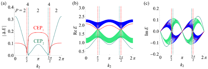
Figure 9: Spectrum properties of NH Lieb lattice on a cylinder at $\pi$ flux. (a) Complex energy gap closings between chiral edge pairs and bulk skin modes. CEP₁ and CEP₂ correspond to the edge modes at $i=1,3$ or equivalently $(+,+)$ and $(+,-)$; (b)-(c) Real and imaginary energy spectra at $\text{Re}E>0$ of bulk skin modes [$(+,+)$ mode in blue and $(+,-)$ mode in light green] and two chiral edge skin modes (in red and dark green). We take a system size $N_{1}=26$ ($N_{2}=200$) along the OBC (PBC) direction. The parameter path follows the orange arrow in Fig. 8 (a). For each edge skin mode, there are two solutions (red and dark green dashed lines) to $|r^{*}_{L,i}(k_{2})r_{R,i}(k_{2})|=1$ over $k_{2}\in[0,2\pi)$, accompanied by a jump of $2$ in generalized biorthogonal polarization. Across these transition lines, the complex energy gap closes and the chiral edge mode enters the bulk.

With the addition of the effective mass terms in Eq. 86, the chiral symmetry is broken. The GBZ winding number is no longer a good invariant for predicting the gap closings at $\pi$ flux. Yet, one can apply the generalized biorthogonal polarization for hybrid boundary conditions in Eq. 52. Based on four chiral edge skin modes constructed in Eq. 89, we define

$$P(k_{2})=M-\lim_{N_{1}\to\infty}\frac{1}{N_{1}}\sum_{i=1}^{M}|\langle\psi^{\text{edge}}_{L,i}(k_{2})|\sum_{j=1}^{N_{1}}j\cdot\Pi_{j}(k_{2})|\psi^{\text{edge}}_{R,i}(k_{2})\rangle|,\quad M=4.$$ (95)

Here, $\Pi_{j}(k_{2})=\sum_{\lambda\in\tilde{A}}|j,\lambda,k_{2}\rangle\langle j,\lambda,k_{2}|$ with $|j,\lambda,k_{2}\rangle=c^{\dagger}_{j,\lambda}(k_{2})|0\rangle$. Due to $\pi$ flux, the polarization varies with $k_{2}$ in contrast to being independent of $k_{\parallel}$ at $0$ flux in Eq. 52. Meanwhile, as shown in Fig. 8 (b), the quantization of $P(k_{2})$ is still well-defined for different system sizes. By further varying one of the hopping parameters, Fig. 8 (a) depicts the pattern of polarization over the $(t_{1},k_{2})$-space, the boundaries of which are captured by $|r^{*}_{L,l}(k_{2})r_{R,l}(k_{2})|=1$. Taking into account the four edge skin modes form two CEPs, each sharing the same localization length, $P(k_{2})$ jumps by $2$ or $4$ every time it crosses the phase boundary. To restore bulk-boundary correspondence for NH bulk and edge skin modes, we introduce the complex energy gap at each $k_{2}$, analogous to the surface energy gap under complete OBC:

$$|\Delta E(k_{2})|=\min_{\forall k_{1}}\{|E_{\text{bulk}}(k_{1},k_{2})-E_{\text{edge}}(k_{2})|\}.$$ (96)

Fig. 9 (a) shows the complex energy gap closings at the transition lines $|r_{R,i}(k_{2})r^{*}_{L,i}(k_{2})|=1$ where the polarization of the chiral edge skin modes jumps.

One can also extend the Amoeba formulation to the cylinder of codimension $d_{c}=1<d$, following the general approach in Eq. 53. As a function of $k_{2}$, the generalized Amoeba is reduced to 1D, capable of predicting complex energy gap closings of chiral edge skin modes. We define $\mathcal{A}_{f}(k_{2})=\{\mu(k_{2})=\log|\beta(k_{2})|:f(\beta,k_{2})=0\}$ where $f(\beta,k_{2})=\det[H(\beta,k_{2})-E]/E^{2}$ and $H(\beta,k_{2})$ is given by the Bloch Hamiltonian in Eq. 93 with the replacement $e^{ik_{1}/2}\to\beta$, in consistency with the magnetic BZ: $k_{1}/2\in(0,\pi/2)$. Two zero-energy bulk flat bands are excluded by the denominator. The Amoeba is solvable in 1D. From $f(\beta,k_{2})=0$, one obtains $\beta_{\pm}(k_{2})=(-b\pm\sqrt{b^{2}-4ac})$/(2a) with $a=(t_{1}^{+}t_{2}^{+})^{2}$, $b=-[(E^{2}-\sum_{l=1}^{4}t_{l}^{+}t_{l}^{-})^{2}-2t_{1}^{+}t_{1}^{-}t_{2}^{+}t_{2}^{-}-(t_{3}^{+}t_{4}^{+}e^{ik_{2}}+t_{3}^{-}t_{4}^{-}e^{-ik_{2}})^{2}]$ and $c=(t_{1}^{-}t_{2}^{-})^{2}$. The two solutions become degenerate at $b^{2}-4ac=0$, indicating an absence of a Amoeba hole. Choosing the reference energy $E$ at the eigenenergy of one of the four chiral edge skin modes, it can be checked that

$$E=\epsilon_{i}(k_{2}):\quad\beta_{+}(k_{2})=\beta_{-}(k_{2})=-\frac{t_{1}^{-}t_{2}^{-}}{t_{1}^{+}t_{2}^{+}}=-r,\quad\text{at}\quad|r^{*}_{L,i}(k_{2})r_{R,i}(k_{2})|_{k_{2}=k_{2,c}}=1.$$ (97)

As expected, the Amoeba hole closes when the corresponding chiral edge skin mode enters the bulk [compare Fig. 9 (a)-(b) with Fig. 10 (a)]. The transition is accompanied by a jump of polarization, demonstrating the consistency of the two approaches for predicting gap closings of boundary modes of codimension zero. Moreover, the center of the Amoeba hole is located at $\mu_{c}=\log|r|$ linked to the imaginary momentum shift in the GBZ. Fig. 10 (c) also shows the Ronkin function descends quickly from a line of minima to a single minimum at $(k_{2,c},\mu_{c})$ where the Amoeba hole disappears.

To conclude, from the simplest example on a cylinder, the biorthogonal polarization and the Amoeba formulation we generalize to hybrid boundary conditions prove to be robust analytical tools to study the interplay between the bulk and higher-order boundary skin modes. The introduction of $\pi$ flux with the magnetic field enriches the phase diagram and creates more diverse types of chiral edge skin modes, as well as more intricate structure in the NH bulk flat band, which leaves possibilities for future exploration.

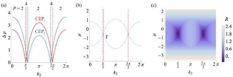
Figure 10: Generalized Amoeba on a cylinder as a function of $k_{2}$ in the NH Lieb lattice at $\pi$ flux. In (a), the reference energies are chosen at the eigen energies of two CEPs, the codimension of which becomes zero at given $k_{2}$. Along the same parameter path as the orange arrow in Fig. 8 (a), their Amoeba hole closes where the polarization jumps, both predicting a complex gap closing with the bulk. In (b) and (c), we take the reference energy from the spectrum of the chiral edge mode $(+,+)$ belonging to CEP₁. At $\Gamma$ points (gray), given by $\Gamma=(k_{2,c},\mu_{c})$, $\mu_{c}=\log(|r|)$ and $|r^{*}_{L_{1}}(k_{2,c})r_{R_{1}}(k_{2,c})|=1$, the Amoeba hole disappears and the Ronkin function descends to a single mininum. The integral grid for the Ronkin function takes a size $M_{1}=100$. We choose $N_{2}=200$ unit cells in the PBC direction of the cylinder.