Probing SUSY at Gravitational Wave Observatories
Abstract
Under the assumption that the recent pulsar timing array evidence for a stochastic gravitational wave (GW) background at nanohertz frequencies is generated by metastable cosmic strings, we analyze the potential of present and future GW observatories for probing the change of particle degrees of freedom caused, e.g., by a supersymmetric (SUSY) extension of the Standard Model (SM). We find that signs of the characteristic doubling of degrees of freedom predicted by SUSY could be detected at Einstein Telescope and Cosmic Explorer even if the masses of the SUSY partner particles are as high as about TeV, far above the reach of any currently envisioned particle collider. We also discuss the detection prospects for the case that some entropy production, e.g. from a late decaying modulus field inducing a temporary matter domination phase in the evolution of the universe, somewhat dilutes the GW spectrum, delaying discovery of the stochastic GW background at LIGO-Virgo-KAGRA. In our analysis we focus on SUSY, but any theory beyond the SM predicting a significant increase of particle degrees of freedom could be probed this way.
I Introduction
The Standard Model (SM) of elementary particles successfully describes a plethora of experimental observations. But it is nevertheless regarded as only an effective theory, that has to be extended to a more complete theory, addressing e.g. the origin of neutrino masses, dark matter, the baryon asymmetry of the universe, the stability of the electroweak scale and finally the quantum nature of gravity. One crucial information we are currently lacking is the energy scale at which new physics extends the SM. Future particle colliders like the FCC-hh FCC:2018vvp could discover new particle degrees of freedom with masses up to TeV. In this letter we demonstrate that future gravitational wave (GW) observatories have the potential to discover signs of SM extensions at even higher energy scales, by detecting the effects of the extra particle degrees of freedom on the evolution of the universe.
Supersymmetry (SUSY) may serve as a benchmark for such considerations. It is motivated, among other things, by its ability to resolve or at least ameliorate the hierarchy problem, i.e. the instability of the electroweak scale under quantum corrections. Although a lower mass scale of the predicted superpartner particles, close to the electroweak scale, is favorable by naturalness arguments, there is no upper bound on . As we will show, signs of the doubling of particle degrees of freedom characteristic of SUSY could be probed for superpartner masses up to TeV, far beyond the reach of any currently envisioned collider.
The condition under which the planned GW observatories can have this intriguing reach is that there exists a predicted stochastic GW background (SGWB) that allows to measure deviations of it caused by the impact of the extra particle degrees of freedom on the evolution of the universe. Interestingly, recent pulsar timing array (PTA) measurements pointing at a SGWB at nanohertz frequencies Xu:2023wog ; Antoniadis:2023ott ; NANOGrav:2023gor ; Reardon:2023gzh ; InternationalPulsarTimingArray:2023mzf indicate that such a possibility might indeed exist. In particular, metastable cosmic strings Kibble:1976sj ; Vilenkin:1982hm are among the best-fitting explanations of the PTA data NANOGrav:2023hvm , which has generated some excitement in the particle physics community (see e.g. Antusch:2023zjk ; Buchmuller:2023aus ; Fu:2023mdu ; Lazarides:2023rqf ; Ahmed:2023rky ; Afzal:2023cyp ; Maji:2023fhv ; Ahmed:2023pjl ; Afzal:2023kqs ; King:2023wkm ; Ahmed:2024iyd , and Lazarides:2023ksx ; Yamada:2023thl ; Lazarides:2023bjd ; Pallis:2024mip ; Kume:2024adn for other works on unstable cosmic strings). The preferred parameters for the metastable cosmic strings from the PTA measurements lead to a prediction of a SGWB in reach of various future GW observatories, such as the Laser Interferometer Space Antenna (LISA) Audley:2017drz , Big Bang Observer (BBO) Corbin:2005ny , DECi hertz Interferometer Gravitational wave Observatory (DECIGO) Seto:2001qf ), Einstein Telescope (ET) Sathyaprakash:2012jk and Cosmic Explorer (CE) Evans:2016mbw . If a SGWB from metastable cosmic strings is indeed be confirmed, this opens up the possibility to discover signs of SUSY up to very high .
In our analysis, we first focus on the sensitivity to signs of SUSY assuming metastable cosmic strings with a standard cosmological history, apart from the extra SUSY particle degrees of freedom. We then explore the potential impact of additional late-time entropy production, which could, e.g., be induced by a late-decaying modulus field, leading to a temporary early matter-dominated phase that dilutes the GW spectrum. This dilution may postpone the detection of the SGWB from a metastable cosmic string network in the currently running observatories, i.e. at LIGO-Virgo-KAGRA (LVK) LIGOScientific:2014pky ; VIRGO:2014yos ; KAGRA:2018plz . While our focus is on the implications of SUSY degrees of freedom on the GW spectrum, we emphasize that our results are more general and applicable to any theoretical framework beyond the SM that predicts a substantial increase in particle degrees of freedom.
II Metastable cosmic strings and PTA data
Topological defects Kibble:1976sj ; Vilenkin:2000jqa can be generated during phase transitions in the early universe. The most prominent examples of topological defects are monopoles and cosmic strings. The former emerge, e.g., when a compact simple group, for example in the context of Grand Unified Theories (GUTs), is spontaneously broken into a subgroup containing an Abelian factor, whereas e.g. the breaking of an Abelian group leads to the latter. Monopoles must be diluted away by a phase of cosmic inflation, since their presence would overclose the universe. Cosmic strings, on the other hand, rapidly enter a scaling regime and emit GWs (see e.g. Hindmarsh:1994re ; Auclair:2019wcv ) over a long period in the history of the universe.
Cosmic strings are metastable if these two aforementioned symmetry breaking scales are close by, and the same Abelian factor involved in the monopole formation takes part in the cosmic string production. Metastable strings eventually decay when monopole-antimonopole pairs spontaneously nucleate along the string cores Vilenkin:1982hm . Such decaying strings have the decay rate per string unit length given by Vilenkin:1982hm ; Preskill:1992ck ; Monin:2008mp ; Leblond:2009fq ; Chitose:2023dam
| (1) |
where is the mass of the monopole, is the energy per unit length of the string, and () are the vacuum expectation values corresponding to monopole (string) formation. For the network behaves like a stable string network. Due to the decay at time after network formation, metastable cosmic strings have a distinct characteristic GW spectrum at low frequencies, compared to stable cosmic strings.
As mentioned in the introduction, metastable cosmic string networks offer a compelling interpretation of the latest PTA observations. Indeed CPTA Xu:2023wog , EPTA Antoniadis:2023ott , NANOGrav NANOGrav:2023gor , and PPTA Reardon:2023gzh (see also Ref. InternationalPulsarTimingArray:2023mzf ) found strong evidence for Hellings-Downs angular correlation Hellings:1983fr , suggesting a SGWB in the nanoherz frequency range. These observations point at a string tension within the range , with being Newton’s constant, for , exhibiting a pronounced correlation between the two quantities, as e.g. shown in Fig. 10 of Ref. NANOGrav:2023hvm . A particularly noteworthy aspect is the overlap of the credible interval in the parameter space with the third-generation constraints from the LVK collaboration.111The current LVK bound on the GW amplitude at frequency 25 Hz KAGRA:2021kbb leads to the upper limit of LIGOScientific:2021nrg ; NANOGrav:2023hvm . Moreover, a substantial portion of the credible region aligns well with these constraints, suggesting a preference for and , if standard cosmological history is assumed.
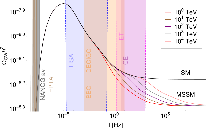
Opposed to other sources of GWs, the spectrum of SGWB originating from (metastable) comic strings is relatively flat over a large frequency range (multiple orders of magnitudes). For a radiation dominated universe with a fixed number of particle species above the electroweak scale it forms a calculable plateau at large frequencies, see Fig. 1. Therefore, it will be possible to fully test whether the observations made by PTAs indeed originate from metastable cosmic strings in GW observatories, including the currently operating detectors LIGOScientific:2014pky ; VIRGO:2014yos ; KAGRA:2018plz , as well as upcoming or planned ones Audley:2017drz ; Corbin:2005ny ; Seto:2001qf ; Sathyaprakash:2012jk ; Evans:2016mbw . It is this property which enables the search for modifications of the cosmic evolution via deviations from the predicted GW spectrum, such as the ones caused by the extra SUSY particle degrees of freedom.
III Effects of SUSY degrees of freedom
In this section, we focus on the effects of the extra SUSY particle degrees of freedom on the GW spectrum of metastable cosmic strings within the minimal supersymmetric SM (MSSM). To compute the spectrum from a cosmic string network, one needs to determine two basic ingredients: (i) the loop number density, which is the number density of sub-horizon sized loops of invariant length at a cosmic time , and (ii) the loop power spectrum, i.e. the emitted power of GWs of frequency by a string having length . The details of these computations are relegated to Appendix A. Both these factors, and therefore the GW spectrum of a cosmic string network, depend non-trivially on the expansion rate of the universe. This cosmological dependence is encoded in the Hubble rate, which reads
| (2) |
with km/s/Mpc, , , and Planck:2018vyg .
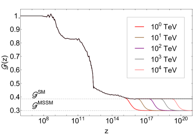
The expansion rate of the universe changes in early times due to the annihilation of relativistic species, which release additional energy into the cosmic plasma, thereby slowing its cooling rate. During the course of this decoupling, entropy is conserved, and the factor that captures the changes in the number of relativistic degrees of freedom is given by
| (3) |
Here, is the effective number of degrees of freedom and is the effective number of entropic degrees of freedom at redshift ( represents redshift today).
Altering the number of degrees of freedom results in smooth variations in the GW spectrum at frequencies that match the temperature at which this modification occurs. The larger the number of degrees of freedom annihilating at a particular temperature, the more prominent the variations in the spectrum. Assuming all SUSY particles have a common mass scale with corresponding temperature (cf. Appendix A for details), one expects a drastic decrease of the number of degrees of freedom by a factor of , leaving an identifiable imprint on the GW spectrum Battye:1997ji ; Cui:2018rwi ; Auclair:2019wcv . The corresponding effect starts to show up at a frequency, , given by Cui:2018rwi ; Auclair:2019wcv
| (4) | ||||
where is used, and temperature (frequency) is given in the unit of GeV (Hz). Moreover, the loop size parameter (defined as ) is , and the total GW power radiated by each loop is (cf. Blanco-Pillado:2017oxo ).
Furthermore, at very high frequencies, the spectrum from a cosmic string network shows a characteristic flat plateau, which deep in the radiation era is given by Blanco-Pillado:2017oxo
| (5) |
The decoupling of the additional degrees of freedom reduces this amplitude of the GW spectrum. The value of the new plateau due to the additional new physics (NP) degrees of freedom can be estimated as Vilenkin:2000jqa ; Cui:2018rwi
| (6) |
In particular, for the MSSM, we have , giving . By measuring the frequency where the GW spectrum starts to show deviations from the cosmic string one in standard cosmology, as well as the characteristic drop of the amplitude towards the new plateau , GW observatories can be sensitive to and .
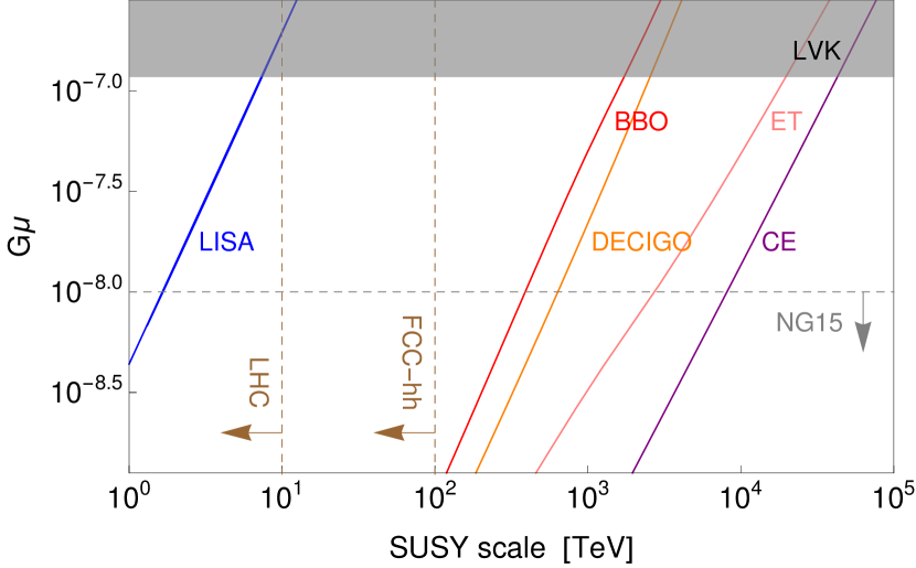
As can be seen from the above formula, , which is preferred to explain the recent PTA dataset, leads to a frequency of Hz for a 3 TeV SUSY scale, which is within the LISA sensitivity (towards the end of the band, to be specific). This is confirmed by our numerical results shown in Fig. 1. Moreover, ET and CE (BBO and DECIGO), having sensitives in the range (), will provide us with the fascinating possibility of probing SUSY scales from the TeV scale to much higher scales. To determine the sensitivity of these experiments we carry out a signal-to-noise ratio (SNR) analysis, where we compare the GW spectrum that includes the SUSY degrees of freedom with the one only incorporating the SM degrees of freedom. We assume standard cosmology and set the detectability threshold to SNR=1 for an observation time of one year. See Appendix B for details of the computational procedure. The results are depicted in Fig. 2. We find that high values of SNR can be obtained in multiple GW detectors. However, Advanced LVK’s (HLVK’s) upcoming observing run, O5, is not sensitive to SUSY degrees of freedom. As can be seen from Fig. 2, LISA is sensitive to the SUSY scale in the muti-TeV range, whereas ET and CE have the potential to detect signs of SUSY up to TeV. Moreover, to determine how exact the number of additional degrees of freedom can be measured from the modified GW spectrum, we perform a Fisher analysis (see Appendix B for details). For we find the Fisher forecast measurement uncertainty of to be less than 10% for TeV ( TeV) at ET (CE). Also, (within the same range of ) we find a Fisher forecast measurement uncertainty of around 5% for the SUSY scale for both ET and CE. Therefore, future GW detectors can access new physics scales far beyond the reach of any planned particle collider.
We have discussed SUSY as characteristic NP example, but of course any theory beyond the SM predicting a significant increase of particle degrees of freedom with up to TeV masses can be probed this way.
IV Effects of Late Time Entropy Production
So far, we have discussed the case that the universe evolves according to standard cosmology, apart from the effects of the extra degrees of freedom, for which we assumed a common mass scale . In the following, we discuss the possibility that late time entropy production, which is a characteristic possibility in SUSY models, affects the SGWB produced from metastable cosmic strings.
For example, when SUSY is broken spontaneously in a hidden sector by the F-term of some chiral superfield, its fermionic component is eaten by the gravitino to generate its mass via the super-Higgs mechanism. But the scalar component, the sgoldstino, remains in the theory and typically has a mass around the gravitino mass. During inflation the sgoldstino is frozen at a field value displaced from its true minimum. When the temperature drops beyond a certain value, the field starts to oscillate and adds a matter-like contribution to the energy density of the universe, which at this time is radiation dominated. Since the matter-like contribution dilutes less than radiation, it can dominate the universe for some time period before it decays. When it decays, it produces entropy that dilutes also the earlier produced GWs.
Other examples of such super-weakly interacting particles, which can produce significant late time entropy (for impacts on cosmology from late decaying particles, see, e.g., Refs. Ellis:1984eq ; Endo:2006zj ; Nakamura:2006uc ; deCarlos:1993wie ; Hasenkamp:2010if ; Co:2016xti ; Apers:2024ffe ), are the gravitinos themselves, moduli fields from string theory, or saxions from a SUSY solution to the strong CP problem. In all these cases it has to be ensured that the late decaying field either has negligible energy, or that it decays before Big Bang Nucleosynthesis (BBN) in order not to spoil the light element distributions (cf. Coughlan:1983ci ), which for only gravitationally interacting particles implies that its mass has to be TeV (for studies of the compatibility of late decaying gravitinos with BBN, see, e.g. Ellis:1986zt ; Moroi:1994rs ; Moroi:1999zb ; Moroi:1999zb ). Since the former case has negligible consequences for the GW spectrum, we focus on the latter.
To investigate the effects of late decaying super-weakly interacting particles on the SGWB from metastable cosmic strings Cui:2017ufi ; Cui:2018rwi ; Auclair:2019wcv ; Gouttenoire:2019kij ; Blasi:2020wpy , we assume an additional matter dominated epoch in the evolution of the otherwise radiation dominated universe before BBN. We assume that the matter domination phase ends at redshift , and gives rise to a dilution factor (i.e. it has started when the scale factor of the universe was a factor smaller than at redshift ). To ensure compatibility with BBN, we consider scenarios where the late decay happens at temperature MeV. Details about the numerical implementation are given in Appendix A.
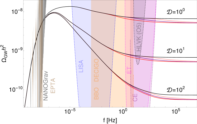
Our numerical results are shown in Fig. 3, demonstrating that the additional matter domination phase can dramatically impact the GW spectrum. The plot shows the case with dilution factors and the undiluted case for comparison, and with TeV. The late decay causes a characteristic break in the GW spectrum, which can be estimated to occur at a frequency given by Cui:2018rwi
| (7) |
where denotes time today, the time of standard matter-radiation equality, is the redshift of standard matter-radiation equality, and is the time where the additional phase of matter domination ends.
We emphasize that due to the drastic drop of for frequencies above , one can raise the value of to without being in conflict with the present LVK bound. Therefore, a perfect fit to the latest PTA data with is possible already with a small dilution factor . A dilution factor of order could delay the discovery of a metastable cosmic string induced SGWB beyond planned HLVK sensitivities, while still remaining in reach of future GW observatories.
It is also important to note that when the dilution factor is large, one can argue that the GW spectrum at large frequencies approaches a GW spectral index Blasi:2020wpy . For we find that the matter domination phase is too short for this characteristic logarithmic slope to develop. This is interesting, because (as long as the logarithmic slope has not reached ) it enhances the possibilities to reconstruct the given model (here specified by , , , and ) from the combined data of future GW observatories. In particular, the maximal logarithmic slope of the spectrum could be used to reconstruct . We furthermore note that the dilution shifts the effects of the SUSY degrees of freedom towards lower frequencies by a factor , whereas smaller would shift these effects to larger frequencies by a factor (cf. Eq. (4)).
Fig. 3 also indicates that the effect of the extra SUSY degrees of freedom could be measurable even in case of dilution from late time entropy production. As commented on in the previous paragraph, this would require to reconstruct the model parameters , , , , e.g. from LISA and PTA results, such that then ET and CE can be sensitive to the extra effect from at . We leave the analysis of the reachable sensitivities in the presence of dilution from late time entropy production to a future work prep , where we will also discuss the impact of lower on the fit to the recent PTA data.
V Conclusions and Summary
Leveraging recent PTA observations of a SGWB at nanohertz frequencies we examine how future GW observatories could detect variations in particle degrees of freedom indicative of SUSY. Under the assumption that the PTA signal originates from metastable cosmic strings, we demonstrate that these detectors could identify the signature doubling of degrees of freedom even for superpartner masses up to TeV. We also discuss scenarios where entropy production, potentially caused e.g. by a late-decaying modulus field leading to an intermediate matter dominated phase, somewhat dilutes the GW spectrum. This would affect the timeline for detecting the GW background with LIGO-Virgo-KAGRA, but could nevertheless allow for detecting a sign of the extra SUSY degrees of freedom with Einstein Telescope and Cosmic Explorer. In summary, if the explanation of the PTA results by metastable cosmic strings is confirmed, future GW observatories open up the intriguing possibility to probe extensions of the SM of elementary particles, like SUSY, up to mass scales far exceeding the reach of current and planned future colliders.
Acknowledgments
We would like to thank Valerie Domcke and Kai Schmitz for fruitful discussions.
oneΔ
Appendix A Computing the GW spectrum of (Meta-)Stable Strings
In this Appendix we describe the used method for computing the GW spectrum of (meta-)stable cosmic strings. It is comprised of three main steps: the determination of the expansion history of the universe, the computation of the loop number density, and, last but not least, using the output of the two previous steps, the computation of the GW spectrum.
For redshift , we take the Hubble rate to be as given by Eq. (2). In this regime . For larger redshift, we neglect sub-leading components of the universe and only keep the dominating fluid. Hence for is initially given by
| (8) |
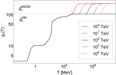
with given by Eq. (3) and . Setting aside a possible period of matter domination, the effect of additional degrees of freedom in thermal equilibrium can then be encoded in and . In the case of the MSSM where all superpartner particles have a common mass we get222We ignore here that neutralinos might have to be treated differently, which, however, depends on the specific model details.
| (9) |
In the regime where and differ substantially, the relation holds, eliminating the need to compute separately. For we have used the values provided by Ref. Husdal:2016haj . Additionally, temperature is needed as a function of redshift, which we determine by the following procedure: First, is computed at some early via
| (10) |
taking advantage of the fact that for small enough . Using , , and entropy conservation we then solve numerically for . In our analysis we approximate with step functions. An example has been illustrated in Fig. 4.
Now, we turn to the inclusion of a phase of matter domination (MD). The picture we have in mind is the following. At early times the universe is radiation dominated (RD), we denote the corresponding energy density by . Additionally there is a subdominant component to the total energy density, denoted by , which scales as matter due to, e.g., a long lived massive particle or a coherently oscillating modulus field. Since and , the matter component will eventually dominate, giving rise to a MD phase. The phase of MD should eventually end, through decay. Hence, we assume that the energy contained in is transferred into , reheating the subdominant radiation component and making it dominant again. The start and end of the phase of MD are in principle determined by the NP model and solving the adequate equations of motion and/or Boltzmann equations. However, we opt to parameterize the phase of MD in a model independent way using the redshift at its end and the dilution factor , see Sec. IV. Going backwards in time, is given by Eq. (8) until , with and being determined as discussed above. For , we take to be
| (11) |
is fixed by requiring to be continuous at . Prior to the phase of MD, is again of the form of (8). Again, is fixed by continuity, the procedure to determine is the straight forward generalization of the one described above. allows for computing and the Hubble radius , which is required for the subsequent steps.
To determine the loop number-density , one has to solve the following partial differential equation Buchmuller:2021mbb :
| (12) |
where is the loop production function. In the above equation, relativistic effects have been neglected, cf. Blanco-Pillado:2013qja ; Buchmuller:2021mbb . Eq. (12) has an analytic solution Buchmuller:2021mbb :
| (13) |
with initial conditions for specified at a time and . As in Ref. Buchmuller:2021mbb , we distinguish between two regimes: early times during which the exponentials can be drooped, and late times where justified by the fact that the cosmic strings network producing loops will have disappeared due to monopole nucleation. The solution Eq. (13) then simplifies to
| (14) |
where
| (15) |
For the purpose of numerics, it is more convenient to compute
| (16) |
from which can easily be recovered. To incorporate different expansion backgrounds, the integral in Eq. (16) is split into several pieces such that within each piece, corresponds to either Eq. (11) or Eq. (8) with :
| (17) |
is chosen according to whether the universe is in an era of MD or RD. We use the simulation results from Ref. Blanco-Pillado:2013qja :
| (18) | ||||
| (19) |
Note that the second function in Eq. (18) is introduced to cut off the divergence (cf. Blanco-Pillado:2013qja , remark after Eq. (30)), other regulators are in principle possible.
Integrals corresponding to a period of MD have been evaluated numerically, however in the case of RD one can easily derive an analytic expression. During one particular integration interval of Eq. (17) the scale factor and the Hubble radius are given by
| (20) |
where and can be determined from the requirement that and should be continuous functions. The result is given by
| (21) |
where
and
| (22) |
and are numerical constants defined as and , respectively. Note that when taking the limit of an eternally radiation dominated universe, i.e. , , , and , and taking advantage of one recovers the loop number density of Blanco-Pillado:2013qja . It is also possible to recover the expression in Eq. (37) of Ref. Blanco-Pillado:2017oxo . The benefit of our approach is that it allows for the epochs being arbitrarily small, whereas the authors of Ref. Blanco-Pillado:2017oxo implicitly assume which only holds asymptotically. Additionally, the true is typically larger than . Since enters with the fifth inverse power into equation Eq. (21) this can lead to an additional suppression. Finally, the GW spectrum is evaluated via
| (23) |
We have evaluated the sum using the method proposed in the Appendix of Ref. Blanco-Pillado:2017oxo and used the coefficients from the same reference.
Appendix B Statistical Analysis
In this Appendix, we discuss the details of the data analysis method adopted in the main text. The GW signal emanating from a cosmic string is given in terms of the GW energy density spectrum, , as a function of frequency. While the instantaneous sensitivity of a GW experiment is characterized in terms of the noise spectrum, . Possessing both spectra enables an evaluation of the likelihood that the anticipated signal will be detected in an experiment. Commonly, this assessment is carried out through computing the SNR, defined as Allen:1996vm ; Allen:1997ad ; Maggiore:1999vm ; Romano:2016dpx
| (24) |
Here the integration is taken over the experiment’s accessible frequency range and its total observing time . For an observation time of years, when SNR is obtained one can deduce that the corresponding GW experiment possesses the capability to detect the anticipated GW signal. For finding the SNR, we compute from our theory predictions, and for , we use the data provided in Ref. Schmitz:2020syl for various GW facilities.
In order to determine the sensitivity of the additional SUSY degrees of freedom, in Eq. (24) we instead consider the following form of the GW signal Kuroyanagi:2018csn ; Caldwell:2018giq , and perform a -analysis to minimize the corresponding SNR as a function of with fixed additional SUSY degrees of freedom, i.e., . We utilize this statistical method to determine if the difference between the spectra, with and without the additional degrees of freedom, is significant enough relative to the noise to be detected. For experiments which will start taking data after LISA, we assume that LISA has already determined and do not perform a -minimization. Moreover, a Fisher analysis allows estimating how well the number of additional degrees of freedom and their corresponding mass scale can be determined in a given GW observatory. To that end, the Fisher matrix is defined as (see e.g. Tegmark:1996bz )
| (25) |
where denote the parameters of the GW spectrum which are in our case chosen to be , and . The covariance matrix is then given as the inverse of the Fisher matrix.
mltΘ
References
- (1) FCC Collaboration, A. Abada et al., “FCC-hh: The Hadron Collider: Future Circular Collider Conceptual Design Report Volume 3,” Eur. Phys. J. ST 228 no. 4, (2019) 755–1107.
- (2) H. Xu et al., “Searching for the Nano-Hertz Stochastic Gravitational Wave Background with the Chinese Pulsar Timing Array Data Release I,” Res. Astron. Astrophys. 23 no. 7, (2023) 075024, arXiv:2306.16216 [astro-ph.HE].
- (3) J. Antoniadis et al., “The second data release from the European Pulsar Timing Array III. Search for gravitational wave signals,” arXiv:2306.16214 [astro-ph.HE].
- (4) NANOGrav Collaboration, G. Agazie et al., “The NANOGrav 15 yr Data Set: Evidence for a Gravitational-wave Background,” Astrophys. J. Lett. 951 no. 1, (2023) L8, arXiv:2306.16213 [astro-ph.HE].
- (5) D. J. Reardon et al., “Search for an Isotropic Gravitational-wave Background with the Parkes Pulsar Timing Array,” Astrophys. J. Lett. 951 no. 1, (2023) L6, arXiv:2306.16215 [astro-ph.HE].
- (6) International Pulsar Timing Array Collaboration, G. Agazie et al., “Comparing recent PTA results on the nanohertz stochastic gravitational wave background,” arXiv:2309.00693 [astro-ph.HE].
- (7) T. W. B. Kibble, “Topology of Cosmic Domains and Strings,” J. Phys. A 9 (1976) 1387–1398.
- (8) A. Vilenkin, “Cosmological Evolution og Monopoles Connected by Strings,” Nucl. Phys. B 196 (1982) 240–258.
- (9) NANOGrav Collaboration, A. Afzal et al., “The NANOGrav 15 yr Data Set: Search for Signals from New Physics,” Astrophys. J. Lett. 951 no. 1, (2023) L11, arXiv:2306.16219 [astro-ph.HE].
- (10) S. Antusch, K. Hinze, S. Saad, and J. Steiner, “Singling out SO(10) GUT models using recent PTA results,” Phys. Rev. D 108 no. 9, (2023) 095053, arXiv:2307.04595 [hep-ph].
- (11) W. Buchmuller, V. Domcke, and K. Schmitz, “Metastable cosmic strings,” JCAP 11 (2023) 020, arXiv:2307.04691 [hep-ph].
- (12) B. Fu, S. F. King, L. Marsili, S. Pascoli, J. Turner, and Y.-L. Zhou, “Testing realistic SO(10) SUSY GUTs with proton decay and gravitational waves,” Phys. Rev. D 109 no. 5, (2024) 055025, arXiv:2308.05799 [hep-ph].
- (13) G. Lazarides, R. Maji, A. Moursy, and Q. Shafi, “Inflation, superheavy metastable strings and gravitational waves in non-supersymmetric flipped SU(5),” JCAP 03 (2024) 006, arXiv:2308.07094 [hep-ph].
- (14) W. Ahmed, M. U. Rehman, and U. Zubair, “Probing stochastic gravitational wave background from SU(5) U(1)χ strings in light of NANOGrav 15-year data,” JCAP 01 (2024) 049, arXiv:2308.09125 [hep-ph].
- (15) A. Afzal, M. Mehmood, M. U. Rehman, and Q. Shafi, “Supersymmetric hybrid inflation and metastable cosmic strings in ,” arXiv:2308.11410 [hep-ph].
- (16) R. Maji and W.-I. Park, “Supersymmetric U(1)B-L flat direction and NANOGrav 15 year data,” JCAP 01 (2024) 015, arXiv:2308.11439 [hep-ph].
- (17) W. Ahmed, T. A. Chowdhury, S. Nasri, and S. Saad, “Gravitational waves from metastable cosmic strings in the Pati-Salam model in light of new pulsar timing array data,” Phys. Rev. D 109 no. 1, (2024) 015008, arXiv:2308.13248 [hep-ph].
- (18) A. Afzal, Q. Shafi, and A. Tiwari, “Gravitational wave emission from metastable current-carrying strings in E6,” Phys. Lett. B 850 (2024) 138516, arXiv:2311.05564 [hep-ph].
- (19) S. F. King, G. K. Leontaris, and Y.-L. Zhou, “Flipped SU(5): unification, proton decay, fermion masses and gravitational waves,” JHEP 03 (2024) 006, arXiv:2311.11857 [hep-ph].
- (20) W. Ahmed, M. Mehmood, M. U. Rehman, and U. Zubair, “Inflation, Proton Decay and Gravitational Waves from Metastable Strings in Model,” arXiv:2404.06008 [hep-ph].
- (21) G. Lazarides, R. Maji, and Q. Shafi, “Superheavy quasi-stable strings and walls bounded by strings in the light of NANOGrav 15 year data,” arXiv:2306.17788 [hep-ph].
- (22) M. Yamada and K. Yonekura, “Dark baryon from pure Yang-Mills theory and its GW signature from cosmic strings,” JHEP 09 (2023) 197, arXiv:2307.06586 [hep-ph].
- (23) G. Lazarides and C. Pallis, “Probing the supersymmetry-mass scale with F-term hybrid inflation,” Phys. Rev. D 108 no. 9, (2023) 095055, arXiv:2309.04848 [hep-ph].
- (24) C. Pallis, “PeV-Scale SUSY and Cosmic Strings from F-term Hybrid Inflation,” arXiv:2403.09385 [hep-ph].
- (25) J. Kume and M. Hindmarsh, “Revised bounds on local cosmic strings from NANOGrav observations,” arXiv:2404.02705 [astro-ph.CO].
- (26) LISA Collaboration, P. Amaro-Seoane et al., “Laser Interferometer Space Antenna,” arXiv:1702.00786 [astro-ph.IM].
- (27) V. Corbin and N. J. Cornish, “Detecting the cosmic gravitational wave background with the big bang observer,” Class. Quant. Grav. 23 (2006) 2435–2446, arXiv:gr-qc/0512039.
- (28) N. Seto, S. Kawamura, and T. Nakamura, “Possibility of direct measurement of the acceleration of the universe using 0.1-Hz band laser interferometer gravitational wave antenna in space,” Phys. Rev. Lett. 87 (2001) 221103, arXiv:astro-ph/0108011.
- (29) B. Sathyaprakash et al., “Scientific Objectives of Einstein Telescope,” Class. Quant. Grav. 29 (2012) 124013, arXiv:1206.0331 [gr-qc]. [Erratum: Class.Quant.Grav. 30, 079501 (2013)].
- (30) LIGO Scientific Collaboration, B. P. Abbott et al., “Exploring the Sensitivity of Next Generation Gravitational Wave Detectors,” Class. Quant. Grav. 34 no. 4, (2017) 044001, arXiv:1607.08697 [astro-ph.IM].
- (31) LIGO Scientific Collaboration, J. Aasi et al., “Advanced LIGO,” Class. Quant. Grav. 32 (2015) 074001, arXiv:1411.4547 [gr-qc].
- (32) VIRGO Collaboration, F. Acernese et al., “Advanced Virgo: a second-generation interferometric gravitational wave detector,” Class. Quant. Grav. 32 no. 2, (2015) 024001, arXiv:1408.3978 [gr-qc].
- (33) KAGRA Collaboration, T. Akutsu et al., “KAGRA: 2.5 Generation Interferometric Gravitational Wave Detector,” Nature Astron. 3 no. 1, (2019) 35–40, arXiv:1811.08079 [gr-qc].
- (34) A. Vilenkin and E. P. S. Shellard, Cosmic Strings and Other Topological Defects. Cambridge University Press, 7, 2000.
- (35) M. B. Hindmarsh and T. W. B. Kibble, “Cosmic strings,” Rept. Prog. Phys. 58 (1995) 477–562, arXiv:hep-ph/9411342.
- (36) P. Auclair et al., “Probing the gravitational wave background from cosmic strings with LISA,” JCAP 04 (2020) 034, arXiv:1909.00819 [astro-ph.CO].
- (37) J. Preskill and A. Vilenkin, “Decay of metastable topological defects,” Phys. Rev. D 47 (1993) 2324–2342, arXiv:hep-ph/9209210.
- (38) A. Monin and M. B. Voloshin, “The Spontaneous breaking of a metastable string,” Phys. Rev. D 78 (2008) 065048, arXiv:0808.1693 [hep-th].
- (39) L. Leblond, B. Shlaer, and X. Siemens, “Gravitational Waves from Broken Cosmic Strings: The Bursts and the Beads,” Phys. Rev. D 79 (2009) 123519, arXiv:0903.4686 [astro-ph.CO].
- (40) A. Chitose, M. Ibe, Y. Nakayama, S. Shirai, and K. Watanabe, “Revisiting metastable cosmic string breaking,” JHEP 04 (2024) 068, arXiv:2312.15662 [hep-ph].
- (41) R. w. Hellings and G. s. Downs, “Upper Limits on the Isotropic Gravitational Radition Background from Pulsar Timing Analysis,” Astrophys. J. Lett. 265 (1983) L39–L42.
- (42) KAGRA, Virgo, LIGO Scientific Collaboration, R. Abbott et al., “Upper limits on the isotropic gravitational-wave background from Advanced LIGO and Advanced Virgo’s third observing run,” Phys. Rev. D 104 no. 2, (2021) 022004, arXiv:2101.12130 [gr-qc].
- (43) LIGO Scientific, Virgo, KAGRA Collaboration, R. Abbott et al., “Constraints on Cosmic Strings Using Data from the Third Advanced LIGO–Virgo Observing Run,” Phys. Rev. Lett. 126 no. 24, (2021) 241102, arXiv:2101.12248 [gr-qc].
- (44) Planck Collaboration, N. Aghanim et al., “Planck 2018 results. VI. Cosmological parameters,” Astron. Astrophys. 641 (2020) A6, arXiv:1807.06209 [astro-ph.CO]. [Erratum: Astron.Astrophys. 652, C4 (2021)].
- (45) R. A. Battye, R. R. Caldwell, and E. P. S. Shellard, “Gravitational waves from cosmic strings,” in Conference on Topological Defects and CMB, pp. 11–31. 6, 1997. arXiv:astro-ph/9706013.
- (46) Y. Cui, M. Lewicki, D. E. Morrissey, and J. D. Wells, “Probing the pre-BBN universe with gravitational waves from cosmic strings,” JHEP 01 (2019) 081, arXiv:1808.08968 [hep-ph].
- (47) J. J. Blanco-Pillado and K. D. Olum, “Stochastic gravitational wave background from smoothed cosmic string loops,” Phys. Rev. D 96 no. 10, (2017) 104046, arXiv:1709.02693 [astro-ph.CO].
- (48) J. R. Ellis, J. E. Kim, and D. V. Nanopoulos, “Cosmological Gravitino Regeneration and Decay,” Phys. Lett. B 145 (1984) 181–186.
- (49) M. Endo, K. Hamaguchi, and F. Takahashi, “Moduli-induced gravitino problem,” Phys. Rev. Lett. 96 (2006) 211301, arXiv:hep-ph/0602061.
- (50) S. Nakamura and M. Yamaguchi, “Gravitino production from heavy moduli decay and cosmological moduli problem revived,” Phys. Lett. B 638 (2006) 389–395, arXiv:hep-ph/0602081.
- (51) B. de Carlos, J. A. Casas, F. Quevedo, and E. Roulet, “Model independent properties and cosmological implications of the dilaton and moduli sectors of 4-d strings,” Phys. Lett. B 318 (1993) 447–456, arXiv:hep-ph/9308325.
- (52) J. Hasenkamp and J. Kersten, “Leptogenesis, Gravitino Dark Matter and Entropy Production,” Phys. Rev. D 82 (2010) 115029, arXiv:1008.1740 [hep-ph].
- (53) R. T. Co, F. D’Eramo, and L. J. Hall, “Supersymmetric axion grand unified theories and their predictions,” Phys. Rev. D 94 no. 7, (2016) 075001, arXiv:1603.04439 [hep-ph].
- (54) F. Apers, J. P. Conlon, E. J. Copeland, M. Mosny, and F. Revello, “String Theory and the First Half of the Universe,” arXiv:2401.04064 [hep-th].
- (55) G. D. Coughlan, W. Fischler, E. W. Kolb, S. Raby, and G. G. Ross, “Cosmological Problems for the Polonyi Potential,” Phys. Lett. B 131 (1983) 59–64.
- (56) J. R. Ellis, D. V. Nanopoulos, and M. Quiros, “On the Axion, Dilaton, Polonyi, Gravitino and Shadow Matter Problems in Supergravity and Superstring Models,” Phys. Lett. B 174 (1986) 176–182.
- (57) T. Moroi, M. Yamaguchi, and T. Yanagida, “On the solution to the Polonyi problem with 0 (10-TeV) gravitino mass in supergravity,” Phys. Lett. B 342 (1995) 105–110, arXiv:hep-ph/9409367.
- (58) T. Moroi and L. Randall, “Wino cold dark matter from anomaly mediated SUSY breaking,” Nucl. Phys. B 570 (2000) 455–472, arXiv:hep-ph/9906527.
- (59) Y. Cui, M. Lewicki, D. E. Morrissey, and J. D. Wells, “Cosmic Archaeology with Gravitational Waves from Cosmic Strings,” Phys. Rev. D 97 no. 12, (2018) 123505, arXiv:1711.03104 [hep-ph].
- (60) Y. Gouttenoire, G. Servant, and P. Simakachorn, “Beyond the Standard Models with Cosmic Strings,” JCAP 07 (2020) 032, arXiv:1912.02569 [hep-ph].
- (61) S. Blasi, V. Brdar, and K. Schmitz, “Fingerprint of low-scale leptogenesis in the primordial gravitational-wave spectrum,” Phys. Rev. Res. 2 no. 4, (2020) 043321, arXiv:2004.02889 [hep-ph].
- (62) S. Antusch, K. Hinze, S. Saad, and J. Steiner ,in preparation .
- (63) L. Husdal, “On Effective Degrees of Freedom in the Early Universe,” Galaxies 4 no. 4, (2016) 78, arXiv:1609.04979 [astro-ph.CO].
- (64) W. Buchmuller, V. Domcke, and K. Schmitz, “Stochastic gravitational-wave background from metastable cosmic strings,” JCAP 12 no. 12, (2021) 006, arXiv:2107.04578 [hep-ph].
- (65) J. J. Blanco-Pillado, K. D. Olum, and B. Shlaer, “The number of cosmic string loops,” Phys. Rev. D 89 no. 2, (2014) 023512, arXiv:1309.6637 [astro-ph.CO].
- (66) B. Allen, “The Stochastic gravity wave background: Sources and detection,” in Les Houches School of Physics: Astrophysical Sources of Gravitational Radiation, pp. 373–417. 4, 1996. arXiv:gr-qc/9604033.
- (67) B. Allen and J. D. Romano, “Detecting a stochastic background of gravitational radiation: Signal processing strategies and sensitivities,” Phys. Rev. D 59 (1999) 102001, arXiv:gr-qc/9710117.
- (68) M. Maggiore, “Gravitational wave experiments and early universe cosmology,” Phys. Rept. 331 (2000) 283–367, arXiv:gr-qc/9909001.
- (69) J. D. Romano and N. J. Cornish, “Detection methods for stochastic gravitational-wave backgrounds: a unified treatment,” Living Rev. Rel. 20 no. 1, (2017) 2, arXiv:1608.06889 [gr-qc].
- (70) K. Schmitz, “New Sensitivity Curves for Gravitational-Wave Signals from Cosmological Phase Transitions,” JHEP 01 (2021) 097, arXiv:2002.04615 [hep-ph].
- (71) S. Kuroyanagi, T. Chiba, and T. Takahashi, “Probing the Universe through the Stochastic Gravitational Wave Background,” JCAP 11 (2018) 038, arXiv:1807.00786 [astro-ph.CO].
- (72) R. R. Caldwell, T. L. Smith, and D. G. E. Walker, “Using a Primordial Gravitational Wave Background to Illuminate New Physics,” Phys. Rev. D 100 no. 4, (2019) 043513, arXiv:1812.07577 [astro-ph.CO].
- (73) M. Tegmark, A. Taylor, and A. Heavens, “Karhunen-Loeve eigenvalue problems in cosmology: How should we tackle large data sets?,” Astrophys. J. 480 (1997) 22, arXiv:astro-ph/9603021.