Generated Contents Enrichment

Abstract

In this paper, we investigate a novel artificial intelligence generation task, termed as generated contents enrichment (GCE). Different from conventional artificial intelligence contents generation task that enriches the given textual description implicitly with limited semantics for generating visually real content, our proposed GCE strives to perform content enrichment explicitly on both the visual and textual domain, from which the enriched contents are visually real, structurally reasonable, and semantically abundant. Towards to solve GCE, we propose a deep end-to-end method that explicitly explores the semantics and inter-semantic relationships during the enrichment. Specifically, we first model the input description as a semantic graph, wherein each node represents an object and each edge corresponds to the inter-object relationship. We then adopt Graph Convolutional Networks on top of the input scene description to predict the enriching objects and their relationships with the input objects. Finally, the enriched graph is fed into an image synthesis model to carry out the visual contents generation. Our experiments conducted on the Visual Genome dataset exhibit promising and visually plausible results.

I Introduction

Given the rich semantics and complex inter-semantic relationships in the real-world scenes in Fig. LABEL:fig:teaser(f), their available descriptions, shown in Fig. LABEL:fig:teaser(a), are usually inadequately informative, thus leading to the semantic richness gap between the accordingly generated images and the real-world ones, as shown in Fig. LABEL:fig:teaser(d) and (f). However, given the simple descriptions, our human minds can easily hallucinate a semantically abundant image, filling the semantic richness gap by first understanding the given description, then enriching it with its related semantics and inter-semantic relationships, and finally hallucinating the accordingly generated image.

We term this task, barely investigated in conventional research, as generated contents enrichment (GCE). Although the human brain can fulfill this task effortlessly, existing artificial intelligence content generation methods produce results with inadequate semantic richness. In contrast to our approach, these methods overlook explicit content enrichment by neglecting reasoning on relevant semantics and inter-semantic relationships. As shown in Fig. LABEL:fig:teaser(d), the state-of-the-art generation approach [2], without reasoning the related semantics of the given descriptions, generates the images with insufficient semantics compared with the real-world ones in Fig. LABEL:fig:teaser(f). Indeed, all existing content generation methods, to the best of our knowledge, rely on implicit learning to generate visual contents that follow the distribution of visually real images without explicitly considering the semantic richness and structural reasonableness, thus incompetent in tackling GCE.

Although GCE is essential for filling the semantic richness gap between the short description and the expected image, it is challenging to learn to solve it. Firstly, the enriching content should be semantically relevant to the ones in the description and form appropriate inter-semantic relationships. Secondly, the enriched scene graph, composited by the description and its enriched semantics, should be structurally real, which follows the distribution of scene graphs from real-world images. Thirdly, since the existing text-to-image generation methods cannot ensure preserving all the textual information in their generated image, the synthesized image from GCE should reflect the input description during the enrichment process.

Towards solving the mentioned challenges and achieving GCE, we propose an intriguing approach that, to some extent, mimics the human reasoning procedure for hallucinating the enriching content. Particularly, our introduced method is designed with an end-to-end trainable architecture consisting of three principal stages. As an initial step, we represent the input description as a scene graph, wherein each node resembles a semantic, i.e., an object, and each edge corresponds to an inter-object relationship. In the first stage, we enrich the scene graph iteratively. In each iteration, we append a single object by modeling it as an unknown node and its related inter-object relationships as unknown edges, which are then predicted employing a Graph Convolutional Network (GCN) by aggregating the information from the known nodes and edges; thus, the enriching contents are semantically relevant with the ones in the description. Then, the enriched scene graph is fed into a pair of Scene Graph Discriminators to guarantee its structural reality. In the second stage, we synthesize the enriched image from the enriched scene graph by adopting an image generator [3]. The third stage simultaneously feeds the enriched image and the input description into the Visual Scene Characteriser and Image-Text Aligner, respectively, thus the generated image is visually real and preserves the information of the description.

Therefore, our contribution is a novel end-to-end trainable framework appointed to handle the proposed GCE task as the first attempt, to our best knowledge. This is executed by demonstrating the input scene descriptions as scene graphs and then enriching the semantics by employing GCNs. Afterward, the final enrichments are produced by feeding the enriched scene graphs into an image generator. In contrast to traditional text-to-image generation approaches, which solely focus on visual authenticity, we enhanced the generation by incorporating explicit visual and textual content enrichments that are semantically and structurally coherent with the provided input description. We assess our method on the real-world images and scene descriptions with rich semantics from the Visual Genome dataset [1], and achieve encouraging quantitative and qualitative outcomes.

II Related Work

II-A Realistic Image Generation

Generative Adversarial Networks (GANs) [4, 5] jointly train a generator and discriminator to distinguish real from fake synthesized images. GANs produce images of high quality that are, in some cases, almost impossible for humans to discriminate from real images [6, 7, 8, 9]. However, their training procedure is not as stable as the other methods, and they may not model all parts of the data distribution [10]. The first attempts for GAN-based text-to-image synthesis [11, 12] are followed by stacking GANs [13] and employing the attention mechanism [14, 15, 16]. Variational Auto Encoder (VAE) [17] consists of an encoder to a latent space and a decoder to return to the image space. VAE is also employed for image synthesis [18, 19], generating high-resolution data but with lower quality than their GAN counterpart. Alternatively, autoregressive approaches [20, 21, 22, 23, 24] synthesize pixels conditioned on an encoded version of the input description that could depend on the previously generated pixels with computationally expensive training and sequential sampling process. Although state-of-the-art diffusion-based [25] models [26, 27, 28, 29] synthesize images of astounding quality, these architectures necessitate elevated computational costs during training and a time-consuming inference. Stable Diffusion [2] is one of the first open-source methods that attracted so much attention among artists as it applies the diffusion process to low-dimensional image embeddings. On the other hand, there has been some research on a hybrid two-stage method like VQ-VAEs [30, 31] and VQGANs [32, 33] which aims to benefit from a mixed version of the mentioned methods.

II-B Graph Neural Networks (GNNs)

Neural networks were first applied to graphs in [34] and further explored in subsequent studies such as [35, 36, 37, 38]. Following improvements in computer vision tasks stemming from the introduction of CNNs, convolution-based models for processing graphs were proposed and divided into two main categories: spectral-based [39, 40, 41, 37, 42] and spatial-based [43, 44, 45, 46]. GNNs may handle many different tasks [47], such as clustering the graph nodes [48], predicting edges between nodes [48], and partitioning the graph [49]. Other GNN applications include but are not limited to text or document classification or capturing the internal structure of text [50, 51], machine translation [52], recommender systems [53, 54], programming [55, 56], predicting social influence [57], preventing adversarial attacks [58], brain networks [59], combinatorial optimization [60], detecting events [61], chemistry-related tasks such as understanding the molecular fingerprints [62], predicting a structure’s properties [46], generating new chemical structures [63, 64], and even predicting the taxi demand [65]. Specifically in Computer Vision, GNNs are employed to tackle human activity recognition [66, 67], processing 3D point clouds [68, 69], interactions of humans and objects [70], image classification with only a few samples [71], question answering [72], visual reasoning [73], and semantic segmentation [74].

II-C Scene Graphs

Scene graphs proposed in [75] and further investigated in [76, 77, 78] are a structured version of a scene representation containing information about objects, their relationships, and often their attributes. Previously, understanding a scene was limited to detecting and recognizing the objects in an image. However, scene graphs aim to obtain a higher level of scene understanding [79] and are employed to improve action recognition [80], image captioning [81], and retrieve images [82]. Also, scene graphs may be predict from images [83, 84, 85, 86, 87, 88] and serve as inputs to generate synthesized images [3, 89, 90, 91, 92].

II-D Semantic Expansion

In prior literature, [93] addresses image outpainting by performing semantic extension applied to a scene graph constructed from a provided input image. Compared to the GCE task, they attempt to solve a separate problem, leading to different objectives and assessment criteria. In other words, we introduce and confront GCE, aiming to enhance the image synthesis quality. This is performed by enriching the same scene described by an input text description by incorporating supplementary related semantics and content.

III Method

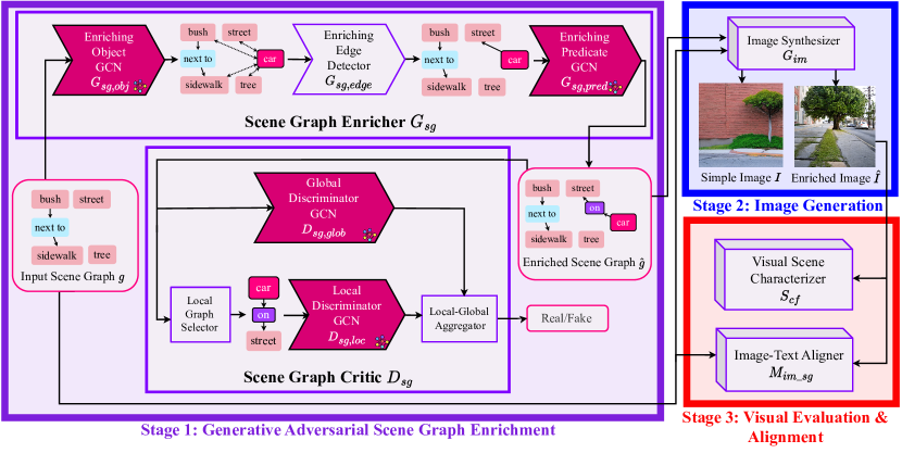
Figure -1: High-Level Overview of our end-to-end Generated Contents Enrichment framework. In Stage 1, the input scene graph (SG) is fed to the Scene Graph Enricher ${G_{sg}}$ to produce an enriched SG. Besides, a pair of local and global discriminators in the SG Critic $D_{sg}$ are jointly trained to differentiate between original and enriched SGs. These discriminators aid the enrichment process in constructing realistic, structurally coherent, and semantically meaningful scenes. In Stage 2, the Image Synthesizer $G_{im}$ leverages the resultant enriched SG to generate an image. In Stage 3, essential visual and textual scene characteristics are extracted in the Visual Scene Characterizer $S_{cf}$ and the Image-Text Aligner $M_{im\_sg}$. These two components ensure that the enriched image appropriately reflects the original description’s inherent characteristics.

Fig. -1 illustrates a high-level representation of our end-to-end model accepting a scene graph (SG) $g$ as input to simultaneously enrich the content in both textual and visual domains. Our proposed approach for GCE consists of three stages performed iteratively.

Initially, Stage 1: Generative Adversarial SG Enrichment accomplishes content enrichment at the object level leveraging Graph Convolutional Networks (GCNs). The SG Enricher, functioning as our generator, employs GCNs and Multi-Layer Perceptrons (MLPs) to identify the enriching objects and their inter/intra-relationships. The SG Critic, as a pair of local and global discriminators, ensures the enriched parts are realistic, structurally coherent, and semantically meaningful both on their own and within the context of the entire graph that represents the scene as a whole. Eventually, the enriched scene graph advances to Stage2: Image Generation, where it serves as the basis for synthesizing an enriched image containing richer relevant content. Lastly, this enriched image, combined with the input SG, progresses to Stage 3: Visual Evaluation & Alignment. Here, we aim to guarantee that the final generated output is visually plausible and faithfully reflects the fundamental scene characteristics outlined in the input prompt. This process involves the employment of a scene classifier and a pair of image/text encoders.

Furthermore, it is important to note that in scenarios where Ground Truth (GT) is unavailable, such as during inference time, both Stage 3: Visual Evaluation & Alignment and the SG Critic are detached from the network.

III-A Scene Graphs

The input scene graph denoted as $g$ consists of two sets, namely $(O,E)$, accompanied by their corresponding features. Here, $O=\{o_{1},\ldots,o_{n}\}$ signifies the set of objects and $E\subseteq O\times\mathcal{R}\times O$ is the set of edges, where $\mathcal{R}$ is the set of all relationship categories. Each individual object is represented as $o_{i}\in\mathcal{C}$, wherein $\mathcal{C}$ is the set of all object categories. Additionally, each edge assumes the form of $(o_{i},r,o_{j})$, where $o_{i},o_{j}\in O$, and the predicate $r\in\mathcal{R}$ describes the relationship type. Within the triplet $(o_{i},r,o_{j})$, $o_{i}$ takes on the role of the relationship’s subject, $o_{j}$ functions as the object of the relationship, and $r$ operates as the predicate characterizing the relationship itself. In other words, this formulation essentially employs a directed edge connecting two nodes, where the relationship’s nature is encapsulated by the relationship category acting as the predicate.

III-B Graph Convolutional Network

Our Graph Convolutional Network (GCN) is inspired by SG2IM [3] and shares similarities with Convolutional Neural Networks (CNNs) in various aspects. Though GCNs are primarily designed to process graphs as inputs, they have the capacity to produce an output graph with a structure similar to the input. This is analogous to CNNs employing appropriate paddings. Each GCN is composed of multiple graph convolution (GConv) layers utilized to aggregate the data from nodes and edges, enabling the propagation of information throughout the graph. In this framework, the $l^{th}$ GConv layer, denoted as $GConv^{(l)}$ performs the message-passing as:

$$\begin{split}(V_{O}^{(l+1)},V_{R}^{(l+1)})=GConv^{(l)}(V_{O}^{(l)},V_{R}^{(l)},O,E).\end{split}$$ (1)

In the context of the $GConv^{(l)}$ input graph, $V_{O}^{(l)}$ represents the feature vectors for all nodes, and $V_{R}^{(l)}$ denotes the feature vectors for all predicates. Additionally, the corresponding output vectors are characterized as $V_{O}^{(l+1)}$ and $V_{R}^{(l+1)}$. To initialize the process, $V_{O}^{(0)}$ and $V_{R}^{(0)}$ serve as the initial vector values for the objects and predicates within the GCN input graph.

Like CNNs, our approach employs weight sharing. This design choice allows the GCN to accommodate graphs with an arbitrary number of vertices and edges. Moreover, parallelization is feasible due to the independence of calculations for each node, enhancing computational efficiency.

The fundamental building block of our GCN is the GConv layer. For every object $o_{i}\in O$ and edge $(o_{i},r,o_{j})\in E$, we concatenate the three corresponding sets of feature vectors, which consist of $(v_{i},v_{r},v_{j})$ representing the subject, predicate, and object vectors, respectively. These concatenated feature sets are then passed through the GConv layer for further processing, initiating with an MLP represented as $f_{g}$:

$$\begin{split}(\bar{v}_{i},\bar{v}_{r},\bar{v}_{j})=f_{g}(v_{i},v_{r},v_{j}).\end{split}$$ (2)

This is to compute the set of three intermediate subject, predicate, and object vectors $(\bar{v}_{i},\bar{v}_{r},\bar{v}_{j})$. Subsequently, these intermediate vectors are aggregated to form $V_{O}^{(l)}$ and $V_{R}^{(l)}$. Node features $V_{O}^{(l)}$ include the new feature vectors $v^{\prime}_{i}$ for the output nodes and edge features $V_{R}^{(l)}$ consist of the new feature vectors $v^{\prime}_{r}$ for the output predicates:

$$v^{\prime}_{r}=f_{r}(v_{r},\bar{v}_{r}),$$ (3)

$$\begin{split}C_{i}^{s}=\{\bar{v}_{i}|(\bar{v}_{i},\bar{v}_{r},\bar{v}_{j})=f_{g}(v_{i},v_{r},v_{j})\text{ and }(o_{i},r,o_{j})\in E\},\\ C_{i}^{o}=\{\bar{v}_{i}|(\bar{v}_{j},\bar{v}_{r},\bar{v}_{i})=f_{g}(v_{j},v_{r},v_{i})\text{ and }(o_{j},r,o_{i})\in E\},\end{split}$$ (4)

$$v^{\prime}_{i}=f_{o}(v_{i},\frac{1}{|C_{i}^{s}|+|C_{i}^{o}|}\sum_{\bar{v}_{i}\in C_{i}^{s}\cup C_{i}^{o}}\bar{v}_{i}).$$ (5)

Here, $f_{r}$ and $f_{o}$ refer to MLPs that include residual links. Additionally, $C_{i}^{s}$ and $C_{i}^{o}$ represent candidate vectors for node $o_{i}$, corresponding to edges where this node serves as either a subject or an object, respectively. To consolidate these candidate vectors for each node, a mean aggregation operation is applied, forming a single vector $v^{\prime}_{i}$. On the other hand, the predicate vector $\bar{v}_{r}$ is directed through additional neural network layers represented as $f_{r}$, which generate the new vector $v^{\prime}_{r}$ incorporating the effects of the residual link.

For more comprehensive information regarding the structure of our GCN and GConv, including detailed illustrations and further explanations, please refer to Section Method and Fig. 1 in the supplementary material.

III-C Stage 1: Generative Adversarial SG Enrichment

III-C1 SG Enricher.

The Scene Graph Enricher, serving as our SG generator and featured in Fig. -1, encompasses three distinct steps, each tailored to address specific subproblems associated with appending a new object, edges, and predicates. These steps leverage the proposed GCNs along with an Enriching Edge Detector. Here is an overview of the process:

First, Enriching Object GCN $G_{sg,obj}$ takes an input SG $g$ to append an enriching object to the scene. Following the addition of objects in the previous step, Enriching Edge Detector $G_{sg,edg}$ takes the new graph and the hidden object vectors and appends edges to the scene. Finally, Enriching Predicate GCN $G_{sg,pred}$ employs the resulting enriched SG from the previous step to detect the predicates associated with the newly added enriching edges. Together, these three steps progressively enhance the input SG by introducing new objects, edges, and predicates, ultimately enriching the scene’s content iteratively.

Our Scene Graph Enricher $G_{sg}$ processes the input graph $g$ as:

$$\hat{g}=G_{sg}(g).$$ (6)

This operation yields an enriched graph $\hat{g}$. Afterward, $\hat{g}$ is reintroduced into the $G_{sg}$ process, initiating an iterative procedure for further enrichment. This recursive approach allows for the scene’s gradual improvement and refinement.

$G_{sg,obj}$ is modeled with the proposed GCN. Additional layers and skip connections are introduced to deepen the GCN, avoiding issues like vanishing gradients. $G_{sg,obj}$ results in the creation of an enriching object denoted as $\hat{o}$, where

$$\hat{o}=G_{sg,obj}(g).$$ (7)

This newly generated enriching object is then added to the original graph $g$. The augmented graph, consisting of both the original objects and the newly created object, continues to serve as the input for the succeeding steps of the enrichment process.

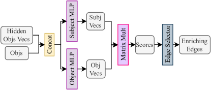
Figure 2: Enriching Edge Detector receives the nodes of a graph but not their edges. It also accepts hidden object vectors from the Enriching Object GCN as input. After concatenation, each node is fed to two neural networks with the same architecture but separate sets of weights to form hidden vectors for subjects and objects of a relationship. This part aims to transfer the nodes to another space where cosine similarity represents the potential of existing edges between two nodes. Therefore, the resulting subject and object vectors form a score matrix implemented as matrix multiplication.

$G_{sg,edg}$ is designed with the utilization of two MLPs $\phi_{s}$ and $\phi_{o}$ sharing the same architecture but with different sets of weights. These MLPs receive several inputs: the initial input node feature vectors $V_{O}^{(0)}$, the enriching object $\hat{o}$, and hidden vectors $V_{O}^{(L)}$ extracted from the final layer of $G_{sg,obj}$. The MLPs $\phi_{s}$ and $\phi_{o}$ are specifically designed to capture information from the objects and subjects, respectively, within the context of directed inter-object relationships. This process is clearly illustrated in Eq. 8 and further elucidated in the supplementary material in Fig. 2.

$$\hat{M}=\phi_{s}(V_{O}^{(0)},v_{\hat{o}},V_{O}^{(L)})\cdot\phi_{o}(V_{O}^{(0)},v_{\hat{o}},V_{O}^{(L)})^{T}$$ (8)

In the Enriching Edge Detector $G_{sg,edg}$, each node vector is transformed into another space to determine the location of the new edges within the enriched graph. These transformed object vectors are then compared using the dot product to detect the enriching edges. The similarity of node features in the new space indicates a higher probability of an edge existing between the two corresponding nodes, as reflected in the entries of $\hat{M}$, similar to an adjacency matrix. Consequently, nodes denoted as $o_{e}$ are selected that form edges $\hat{e}=(o_{e},.,\hat{o})$ or $\hat{e}=(\hat{o},.,o_{e})$, where the notation ”.” signifies a placeholder for the unknown predicate. This selection process for nodes forming enriching edges by considering the similarity of node features in the transformed space is summarized as:

$$\hat{e}=G_{sg,edg}(V_{O}^{(0)},v_{\hat{o}},V_{O}^{(L)}).$$ (9)

After the determination of edges between the enriching node $\hat{o}$ and the pre-existing objects is completed, the newly formed graph $\tilde{g}=\{g,\hat{o},\hat{e}\}$ is then passed to $G_{sg,pred}$. Notably, $G_{sg,pred}$ maintains the same architecture as $G_{sg,obj}$ but operates with an independent set of parameters:

$$\hat{r}=G_{sg,pred}(g,\hat{o},\hat{e}).$$ (10)

$G_{sg,pred}$ is designed with the proposed GCN tasked with producing the type of relationship $\hat{r}$ for each enriching edge $\hat{e}$ derived from the previous step.

Finally, a new graph $\hat{g}$ is assembled by combining the input graph $g$, enriching object $\hat{o}$, the edges $\hat{e}$, and the relationships $\hat{r}$. This comprehensive graph serves as input for the following enrichment iterations and represents the enriched scene with all the appended elements and their associated attributes.

III-C2 SG Critic.

Scene Graph Critic $D_{sg}$, as depicted in Fig. -1, indeed consists of a pair of discriminators trained jointly with the rest of the network. The high-level architecture of this critic draws inspiration from discriminators employed in GAN-based image inpainting [94]. Some additional details regarding the architecture of GCNs are provided in the supplementary materials.

In the global discriminator denoted as $D_{sg,glob}$, a GCN is employed to transform the input into another graph. The extracted features in nodes and edges of this graph are utilized to differentiate the source of input data. Given that our model handles graphs with varying numbers of nodes and edges, an aggregation method such as averaging needs to be utilized at this stage. The output vectors for nodes and edges are separately aggregated and then input into additional neural network layers for further processing and discrimination.

Our global discriminator is deeper compared to the local discriminator represented as $D_{sg,loc}$ by incorporating two additional GConv layers. The local discriminator exclusively receives a subgraph comprising the enriching nodes, their immediate neighbors, and corresponding edges. The outputs of two discriminators are concatenated and subsequently passed through additional layers. This process ultimately culminates in the computation of a score. This score reflects the discrimination of an enriched graph from an original one in our critic’s assessment.

III-D Stage 2: Image Generation

Our base image generator employs a pre-trained image synthesizer [3]. Precisely, the process entails feeding scene graphs to a GCN for object features to be extracted. These extracted features are then utilized to form a scene layout for image synthesis with some convolutional layers. Simultaneously, image discriminators are jointly trained to ensure that the objects within the generated image are recognizable and image patches appear realistic, enhancing the overall quality and coherence of the generated images.

Both the GT scene graph $g_{GT}$ corresponding to the input graph $g$ in addition to the resulting enriched scene graph $\hat{g}$ are provided as input to the image generator $G_{im}$ to produce images $I$ and $\hat{I}$ (Eq. 11). These images further contribute to the overall enrichment objective function.

$$I=G_{im}(g_{GT});\hat{I}=G_{im}(\hat{g}).$$ (11)

III-E Stage 3: Visual Evaluation & Alignment

III-E1 Visual Scene Characterizer.

We need to ensure that the enriched output image, with its additional content, faithfully reflects the essential characteristics outlined in the GT description. Thus, a pre-trained scene classifier $S_{cf}$ [95] receives the generated enriched image $\hat{I}$ to evaluate the mentioned criteria. The hidden scene features for both images $I$ and $\hat{I}$ are extracted (Eq. 12). These extracted features are afterward integrated into the objective function, thus playing a crucial role in the end-to-end training of all components within the framework.

$$h_{I}=S_{cf}(I);h_{\hat{I}}=S_{cf}(\hat{I}).$$ (12)

III-E2 Image-Text Aligner.

The Image-Text Aligner, represented as $M_{im\_sg}$, leverages pre-trained CLIP encoders [96]. It aims to ensure that the enriched generated images accurately reflect the essential scene elements outlined in the input description. This multimodal network operates by accepting both the input graph $g$ and the enriched image $\hat{I}$. It extracts features denoted as $F_{g}$ from the graph and $F_{I}$ from the image:

$$F_{g}=M_{im\_sg}(g);F_{I}=M_{im\_sg}(\hat{I}).$$ (13)

These features are further employed in the objective function.

III-F Objective Function

To train the model end-to-end, one random object is selected from each GT graph $g_{GT}$ to be eliminated along with its connected edges. $G_{sg,obj}$ aims to predict the object category of this removed node, which leads to our Objs Loss,

$$\mathcal{L}_{obj}=\frac{1}{N}\sum_{i=1}^{N}CE(\hat{o}^{(i)},o_{GT}^{(i)}),$$ (14)

where $N$ represents the mini-batch size. This loss is structured as a cross-entropy measure, comparing the predicted object $\hat{o}^{(i)}$ and its GT counterpart $o_{GT}^{(i)}$ in the GT graph $g_{GT}$. In fact, the eliminated object is denoted using an introduced distinct object category labeled as $unknown\_obj$. Additionally, all the potential edges leading to or from this node are included as $unknown\_pred$, a newly introduced predicate category.

$G_{sg,edg}$ produces a matrix $\hat{M}$ which resembles an adjacency matrix. However, each entry $\hat{m}_{i,j}$ within this matrix signifies the probability of an edge existing between $o_{i}$ as a subject and $o_{j}$ as an object. The Enriching Edge Detector contributes to the objective function with Edge Loss,

$$\mathcal{L}_{edg}=\frac{1}{N}\sum_{k=1}^{N}\sum_{i,j}BCE(\hat{m}_{i,j}^{(k)},m^{(k)}_{GT;i,j})$$ (15)

computed as a binary cross-entropy considering whether an edge exists between each pair of nodes in the GT graph, including the enriching object.

Based on $\hat{M}$, one of the edges could be selected, and then its predicate is predicted by $G_{sg,pred}$. In the GT, the predicate for this edge may or may not be provided, leading to the formulation of two supplementary loss terms computed via cross-entropy as Available Preds Loss and Not Avail Preds Loss:

$$\mathcal{L}_{pred,avail}=\frac{1}{N}\sum_{i=1}^{N}CE(\hat{r}^{(i)},r_{GT}^{(i)}),$$ (16)

$$\mathcal{L}_{pred,not\_avail}=\frac{1}{N}\sum_{i=1}^{N}CE(\hat{r}^{(i)},none\_pred),$$ (17)

where the term $none\_pred$ signifies a predicate category analogous to no relationships.

We extract a pair of features from the final layer of the scene classifier, one corresponding to the generated image from the GT scene graph and the other to the enriched synthesized image (Eq. 12). These features are then compared, leading to the alignment process contributing to enrichment. This alignment is to ensure that the appended content is coherent with the high-level essential visual characteristics of the GT. This loss term is denoted by Scene Classifier Loss,

$$\mathcal{L}_{sc}=\frac{1}{N}\sum_{i=1}^{N}||h_{I}^{(i)}-h_{\hat{I}}^{(i)}||_{p},$$ (18)

implemented as $L_{p}$ difference between GT and enriched scene features. Alternatively, it can be modeled as another form of comparison:

$$\mathcal{L}_{sc}=\frac{1}{N}\sum_{i=1}^{N}CE(s_{\hat{I}}^{(i)},s_{I}^{(i)}),$$ (19)

the cross-entropy between the predicted scene classes denoted as $s_{I}$ for image $I$ and $s_{\hat{I}}$ for image $\hat{I}$. This constraint guarantees that the predicted scene classes are identical, thereby signifying that the enrichment content does not modify the high-level scene comprehension of the input description.

The Image-Text Aligner produces a pair of normalized features, denoted as $F_{g}$ and $F_{I}$ both of which share the same dimension (Eq. 20). These features are then used to establish the Image-SG Alignment Loss,

$$\mathcal{L}_{im\_sg}=-\frac{1}{N}\sum_{i=1}^{N}F_{g}^{(i)}\cdot F_{I}^{(i)},$$ (20)

which takes the form of a cosine similarity. This similarity measure is applied to maintain the consistency of the synthesized enriched image in relation to the fundamentals outlined in the original description.

$D_{sg}$ and $G_{sg}$ undergo training within an adversarial setting by engaging in a GAN min-max game. In this setting, the generator and the discriminators have opposing objectives, seeking to minimize and maximize the following loss term, respectively:

$$\mathcal{L}_{GAN}=\mathop{\mathbb{E}}_{g\sim p_{\textrm{real}}}\log D_{sg}(g)+\mathop{\mathbb{E}}_{\hat{g}\sim p_{\textrm{enriched}}}\log(1-D_{sg}(\hat{g}))$$ (21)

Finally, in our end-to-end training process, we opt for a weighted sum $\mathcal{L}$ that encompasses all the previously mentioned loss terms (Eq. 22). This comprehensive objective function promotes the training of the entire framework, ensuring that all components work together cohesively.

$$\begin{split}\mathcal{L}=w_{0}\mathcal{L}_{obj}+w_{1}\mathcal{L}_{edg}+w_{2}\mathcal{L}_{GAN}+w_{3}\mathcal{L}_{pred,avail}\\ +w_{4}\mathcal{L}_{pred,not\_avail}+w_{5}\mathcal{L}_{sc}+w_{6}\mathcal{L}_{im\_sg}\end{split}$$ (22)

A thorough exploration of training specifics and hyperparameter selection can be found in the supplementary materials. This encompasses various configurations for our GCNs’ architectures, mini-batch size, activation functions, dimensions of embedding vectors within the generator and discriminators, dropout layers, normalization techniques, and different combinations of weights for loss terms as defined in Eq. 22.

During the training process, gradients are backpropagated through the pre-trained versions of the image generator, scene classifier, and CLIP encoders. However, it is essential to note that only the parameters associated with $G_{sg}$ and $D_{sg}$ are updated as part of the training procedure.

During the inference phase, an $unknown\_obj$ node along with its corresponding $unknown\_pred$ edges are introduced into the input graph before being passed to $G_{sg}$. The enrichment process can be iteratively performed multiple times to progressively add additional content. At each iteration of this process, images may be generated from the resulting enriched intermediate scene graphs.

IV Experiments

In this section, we aim to establish the coherence between the enriching objects and relationships with the original scene as described by the input scene graph. Additionally, we demonstrate that scene graph enrichment leads to an augmented version of the input graph, ultimately generating richer images. We achieve these through a combination of qualitative illustrations and quantitative results.

IV-A Dataset

For our experiments, we employed the Visual Genome (VG) dataset [1], which comprises approximately 110k images, each accompanied by its corresponding scene graph. We adopted a preprocessing pipeline similar to that in [3] where only objects and relationships with at least 2k and 0.5 occurrences are selected. This resulted in a dataset containing 178 object categories and 45 predicate categories. Consequently, for our training, testing, and validation splits, we retained approximately 62.5k, 5.5k, and 5k data points, respectively.

IV-B ChatGPT Comparison Experiments

In case the input is represented as raw text rather than modeling as scene graphs, Large Language Models (LLMs) may be employed to expand the scene descriptions [97, 98, 99, 100, 101, 102, 103]. However, LLMs cannot efficiently and effectively perform the GCE task. First, simultaneous training of LLMs and image generators demands substantial training data and entails significant computational expenses. Secondly, despite the LLMs’ capacity to enrich the textual information, they lack the ability to comprehend the visual implications of the augmented content and measure its adequacy for generating a single real-world image. Thirdly, the direct utilization of LLMs might result in redundant content generation for image synthesis, particularly given that even the state-of-the-art generation method [2] struggles with handling exceedingly complex prompts.

To illustrate the superiority of our proposed framework over LLMs, we conducted a comparison utilizing ChatGPT [98] for the content enrichment task. This is presented qualitatively in Figure  ‣ IV-B and quantitatively in Table II. The input descriptions are provided to ChatGPT, which generates enriched descriptions that are then used to synthesize images utilizing Stable Diffusion. We limited the word count for ChatGPT output as originally it generates very long texts unsuitable for inputs to SOTA image generators. These three different styles of prompts were used:

• ChatGPT Direct: Please complete this given text so that the final text contains between 15 to 25 words: ”input_description”

• ChatGPT Scene: Please complete this given text describing a scene so that the final text contains between 15 to 25 words: ”input_description”

• ChatGPT Object: Please complete this given text describing a scene with more related objects so that the final text contains between 15 to 25 words: ”input_description”

(a)
Input Text

(b)
Enriched Text
ChatGPT

(c)
Enriched Text
Ours

(d)
Simple Image
(Directly by Input Text)

(e)
Enriched Image
ChatGPT

(f)
Enriched Image
Ours

Railing around Edge. Water. Railing around edge. Water below. A tranquil view, with safety in mind, encapsulates the beauty of this waterfront setting. Railing on sidewalk and around edge. Water. Sky has edge. Tree on sidewalk that has beach, ocean, grass, and cloud.
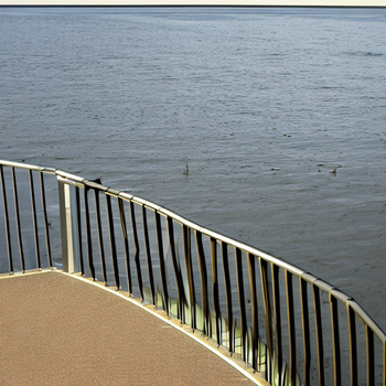
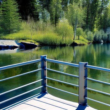
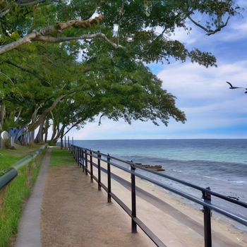
Plate next to bowl. Glass next to bowl Plate and glass next to bowl. The table set for a simple, yet inviting meal, ready to be enjoyed. Plate and glass next to bowl on top of table. Food, cup, leaf, flower, water on top of plate.
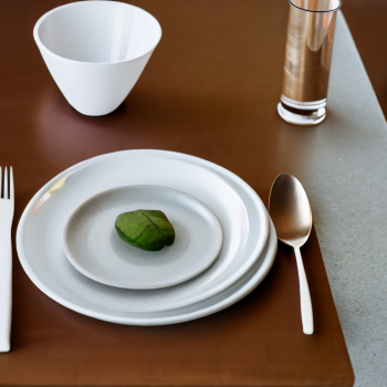
Cloud above water. Reflection on top of water. Cloud above water. Reflection on top of water. The peaceful lake mirrors the sky, creating a serene and beautiful sight. Cloud in mountain. Cloud above water. Reflection on top of water. Sky, tree, building, boat, and house in water.
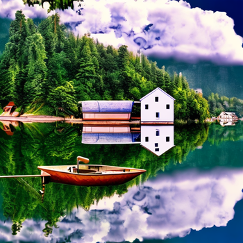
Glass with water. Plate with pizza. Glass with water. Plate with pizza. A delicious meal, with a refreshing drink, awaits, satisfying both thirst and appetite. Glass with water on table. Plate with pizza. Cup, handle, bottle, food, bowl, glasses, and hand on table.
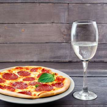
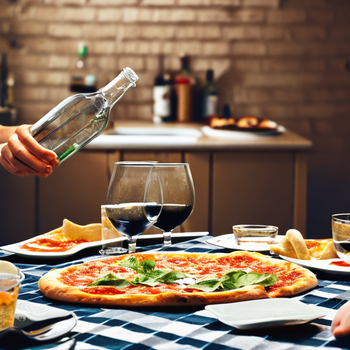
Snow next to road. Snow next to road. A wintry landscape, where the glistening snow adds a touch of magic to the familiar thoroughfare. Snow on top of truck next to road. Sky, tree, sign, line, ground, building, car, cloud, and sidewalk on road.
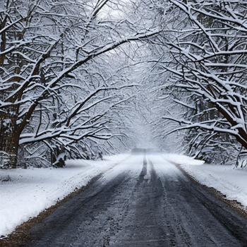
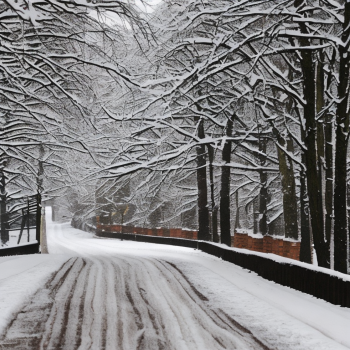
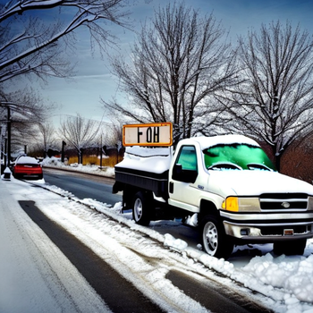
Car. Road near Street. Car. Road near street. An everyday scene where the car navigates the road close to a charming, bustling street. Car. Sign on road near street. Bus and line on street near tree and building. Sky and sidewalk near building.

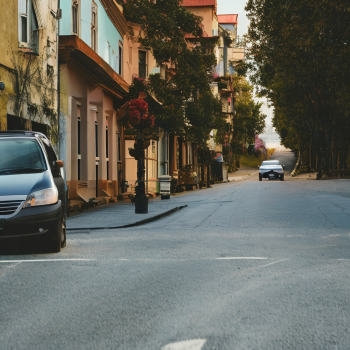
Figure 0: Qualitative Results. Samples of scene descriptions from the Visual Genome test split have been enriched, along with their synthesized images featuring richer content. The simple image is generated directly from the input text, and the enriched images are produced from their corresponding enriched text.

IV-C Qualitative Results

Fig.  ‣ IV-B showcases input descriptions and their enrichments alongside their corresponding synthesized images employing ChatGPT Direct and our proposed model. These input scene graphs are selected from the VG test split. In cases where the original scene graph contains a large number of objects, a subgraph with its associated edges is randomly selected and used as the initial input for our experiments. This subgraph strategy is primarily driven by the limitations of image generators when synthesizing images with lots of objects. Thus, if the initial input description already contains a substantial number of objects, the image synthesizer cannot accurately depict the enriched scene with even more objects. However, it is essential to note that there are no constraints regarding the number of semantics in the input description. Our proposed method carries out semantic enrichment iteratively, focusing on enriching one object at a time in each step, regardless of the number of existing objects in the scene.

To ensure there is no overlap in VG between the data used for training different stages of our model, Stage1: Image Generation is pre-trained on the same train split as ours. Moreover, in Visual Scene Characterizer, we employ a pre-trained residual CNN scene classifier [95]. During network training, the gradients backpropagate through Stage 3: Visual Evaluation & Alignment and Stage2: Image Generation; however, their parameters are not updated, as our objective function is specifically designed to optimize a different problem which is joint SG/image enrichment.

IV-D Quantitative Results

Measure	SG Enrich	Deep G	Best NoD	128 BS
Objs Acc	19.04	17.31	15.09	16.85
Avail Preds Acc	41.95	39.90	40.25	31.38
Not Avail Preds Acc	-	-	3.02	-
Avail Edges Acc	75.00	75.64	76.08	66.89
Not Avail Edges Acc	99.58	99.70	99.54	99.54
Scene Class Acc	20.33	20.84	19.18	25.33

TABLE I: Quantitative Results, including our defined measures for the Generated Contents Enrichment task on scene graphs, is shown for selected hyperparameter configurations. For more detailed information, please refer to the supplementary materials.

Evaluating the performance of SG enrichment presents a non-trivial challenge, given that there is no unique solution. In other words, there are multiple ways to enrich a graph by adding objects and relationships, each leading to a richer generated image with reasonable semantics.

IV-D1 Inpainting Inspired Metrics

Similar to the domain of image inpainting, we may seek simple measures comparing predictions and GT, such as $L_{p}$ distance for pixel values or, in our specific case, accuracy for object and relationship predictions.

As so many terms are encompassed within our loss function, the contribution of each term plays an essential role in the overall enrichment task. For this reason, we conducted comprehensive hyperparameter tuning, and detailed results and discussions can be found in the supplementary materials. This includes the selected hyperparameters corresponding to the models in Table I, providing our quantitative evaluation methods for some of the chosen instances.

We have included Table I to demonstrate that our proposed method is capable of content enrichment in a structurally reasonable manner, as opposed to merely adding random content. It is important to emphasize that the enrichment process is inherently ill-posed since any appropriate enrichment is correct, and the final result is not deterministic. Therefore, the relatively low prediction accuracy does not provide a comprehensive illustration of the real performance of our introduced approach.

The metric Objs Acc represents the accuracy of our prediction among approximately 178 object categories. While it may appear relatively low, it is important to note that this outcome arises from the nature of our task. We randomly eliminate an object from a scene and then attempt to predict it based on the semantics and structure of the scene. Moreover, the GT scene graph is not the only reasonable answer. Thus, different objects, other than the GT, may be appended to form visually plausible enriched images while maintaining the reasonable structure and coherence of the entire scene.

The edge detection task involves binary predictions between every pair of nodes. During the training of the Enriching Edge Detector, predictions are made for all objects in the scene graph, encompassing both the enriching and original objects.

Avail Edges Acc measures the accuracy of predicting the presence of a directed edge between two nodes connected as subject and object in a relationship within the GT graph. Similarly, Not Avail Edges Acc represents the accuracy for edges whose existence is not provided in the GT graph. It is worth mentioning that the absence of an edge in the GT graph does not necessarily imply that predicting such an edge would lead to a description of a different scene. Therefore, any comparisons between the results should be made cautiously, as the problem inherently allows for multiple valid solutions.

In cases where the Enriching Edge Detector fails to accurately predict the existence of an enriching edge compared to the GT, we also penalize the Enriching Predicate GCN. This is achieved using the appropriate loss term and the introduced $none\_pred$ as the GT predicate category. The accuracy of this prediction is denoted as Not Avail Preds Acc, which is included in Table I only if the edge prediction fails for at least one enriching object, as per the GT graph. However, assume the Enriching Edge Detector successfully performs its task based on the GT. Then, we consider the prediction of the Enriching Predicate GCN as Avail Preds Acc. This metric assesses the accuracy of predicting the predicates among approximately 45 different relationship categories.

Scene Class Acc demonstrates whether the scene categories for a pair of images generated from GT and enriched scene graph are the same. During training, images have a lower resolution, and the pre-trained scene classifier does not have a high classification accuracy on its own. Thus, we do not anticipate a high matching accuracy for Scene Class Acc. Though the GT scene category is not unique, our goal is to enrich a scene by appending only one object and its relationships to finally synthesize images with the same essential visual scene characteristics as the GT graph.

IV-D2 Generated Image Quality Metrics

Metric (Reference Distribution)	Simple	Enriched ChatGPT Direct	Enriched ChatGPT Scene	Enriched ChatGPT Object	Enriched Ours	GT Synthesized	VG	Improvement Ours vs. Simple
IS$\uparrow$	17.03 $\pm$ 0.37	15.44 $\pm$ 0.32	14.90 $\pm$ 0.19	15.69 $\pm$ 0.26	19.37 $\pm$ 0.28	24.44$\pm$ 0.32	38.61 $\pm$ 0.52	13.74%
FID$\downarrow$ (GT Synthesized)	37.85	42.15	47.74	52.74	34.89	0	35.32	7.82%
FID$\downarrow$ (VG)	61.27	64.69	68.06	73.48	53.23	35.32	0	13.12%

TABLE II: Inception Scores (IS) [104] and Fréchet Inception Distances (FID) [105] are computed to compare real-world VG dataset and sets of images generated from GT scene descriptions (GT Synthesized), Simple descriptions, and Enriched versions utilizing Our model and ChatGPT with three different prompt styles.

Inception Scores (IS) [104] and Fréchet Inception Distances (FID) [105] are widely recognized metrics used to evaluate the quality of synthesized images. IS relies on a pre-trained image classifier to assess the presence of recognizable objects and their diversity within the generated image set. FID, on the other hand, employs a pre-trained classifier to extract deep features from both generated and real image sets. It then measures the statistical similarity between the distributions of these extracted features for the generated and real image sets.

Table II exhibits FID and IS metrics for evaluating the image quality. Stable Diffusion is employed as the image synthesizer to generate images for different scenarios compared to the real-world VG images:

• First, simple scene descriptions from the test set are utilized for synthesizing a total of 36.5k simple images denoted by Simple.

• Second, the same simple descriptions are fed to our proposed GCE method or ChatGPT with the three introduced prompting styles. This is to produce the enriched descriptions used for synthesizing 36.5k enriched images denoted by Enriched for each of the mentioned four cases: Enriched ChatGPT Direct/Scene/Object and Enriched Ours.

• Third, GT training scene descriptions are directly used to generate 35k images denoted by GT Synthesized.

• The fourth set of images is 87k real-world VG images denoted by VG.

The FID metric is calculated with two different reference distributions denoted by FID [GT Synthesized] and FID [VG]: one considering GT Synthesized images and the other one using VG images as reference distributions, respectively. The results show improvements in both IS and FID metrics for Enriched images compared to Simple ones. This coarsely demonstrates that our enriched images have higher-quality content and similarity to the reference distributions. However, it is important to note that GT Synthesized images maintain better IS and FID metrics than Enriched images. This is because GT Synthesized images are generated directly from the GT training split, which provides more detailed and diverse descriptions. Thus, when using a fixed image synthesizer, GT Synthesized may be considered an upper bound for the enrichment task.

Due to limitations in the VG dataset, our model does not enrich the attributed properties of each object, such as its color. However, these attributes are present in ChatGPT-enriched texts, which adds diversity to the generated images, potentially improving IS and FID. As a result, ChatGPT might be placed in a superior prior position compared to our proposed model. Nonetheless, when evaluating FID and IS, our introduced framework outperforms ChatGPT, which performs worse than even Simple initial descriptions. Notably, as we include specific information related to the task, transitioning from ChatGPT Direct to Scene and then Object, FID scores worsen, indicating that LLMs such as ChatGPT, in their standard out-of-the-box version, are not well-suited for the GCE task. This is primarily due to LLMs generating redundant content for image synthesis without considering the visual implications of the enriched text for producing a realistic image.

Measure	SG Enrich	W/o $D_{sg}$	W/o $D_{sg,glob}$	W/o $D_{sg,loc}$	W/o $S_{cf}$	With $M_{im\_sg}$
Objs Acc	19.04	18.33	18.52	18.66	17.88	19.48
Avail Preds Acc	41.95	37.43	38.87	37.47	36.08	42.20
Not Avail Preds Acc	-	-	-	-	-	-
Avail Edges Acc	75.00	74.89	74.20	75.33	74.62	75.18
Not Avail Edges Acc	99.58	99.61	99.61	99.60	99.66	99.57
Scene Class Acc	20.33	19.99	21.14	21.66	-	22.66

TABLE III: Ablation study results. Modules are altered with respect to SG Enrich as the baseline.

IV-E Ablation Study

In order to demonstrate the necessity of each component in our model and their individual contribution to the overall performance, we conducted an ablation study. The results of this study are presented in Table III, where the ablated models are compared employing our defined metrics for scene graph enrichment. Since this task lacks a unique solution, raw results with the specified metrics may be misleading for comparison and often can contradict human judgments.

The baseline for these studies is the SG Enrich model with hyperparameters and architectures detailed in the supplementary materials. We explore various cases, including eliminating the scene classifier and adding the Image-Text Aligner. The pair of discriminators or each of the local and global discriminators individually is also removed to coarsely indicate their contribution.

In the case labeled W/o $D_{sg}$, we omit the pair of discriminators, effectively eliminating the adversarial GAN loss component, which backpropagates from the discriminators to aid the enrichment process.

W/o $D_{sg,loc}$ and W/o $D_{sg,glob}$ are cases with only global or local discriminators retained, respectively. W/o $D_{sg,loc}$ understands the entire scene without paying specific attention to the enrichments. Although the individual enriched subgraphs may seem realistic in W/o $D_{sg,glob}$, it is incapable of capturing the overall inconsistency between the enriched content and the entire scene.

W/o $S_{cf}$ omits the pre-trained scene classifier in the Visual Scene Characterizer. This component evaluates whether the synthesized images reflect the essential scene characteristics described in the original input. Though some objects in the synthesized images might often not be recognizable for the scene classifier, the related loss term still contributes to the overall performance, helping the model to enrich scenes effectively.

The variant labeled With $M_{im\_sg}$ includes the Image-Text Aligner component, which is not present in our baseline model denoted by SG Enrich. This component comprises the CLIP encoders accountable for ensuring that the generated enriched images accurately reflect the essential scene components described in the original input scene graphs.

IV-F User Studies

S1: Which one of the images is more realistic?
Stable Diffusion Image	Real-World Image	$\pm$ Standard Deviation
20.09%	79.91%	$\pm$ 23.27%
S2: Which one of the images is more realistic?
Enriched Image	Simple Image	$\pm$ Standard Deviation
49.45%	50.55%	$\pm$ 28.30%
S3: Does the image reflect the description?
Yes	No	$\pm$ Standard Deviation
70.82%	29.18%	$\pm$ 13.92%
S4: Based on real image, which AI-generated image do you prefer?
Enriched Image	Simple Image	$\pm$ Standard Deviation
83.40%	16.60%	$\pm$ 12.24%

TABLE IV: User studies are conducted in four sections to evaluate the effectiveness of the enrichment process.

Our efforts to demonstrate the performance of our model and its different variations involved employing our defined metrics and borrowed measures from the assessment of generated image quality. Nevertheless, it is crucial to acknowledge that evaluating the model’s performance solely against GT provides only a rough measure due to the inherently ill-posed nature of the problem. Ultimately, human judgment is essential to truly claim the quality of the enrichment process. In this regard, our user studies, detailed in Table IV, were conducted with the participation of 110 individuals, spanning four sections.

S1: Real vs. Stable Diffusion Images Realisticness. To showcase the capability of our image generator to produce realistic images, we presented users with ten pairs of images. Each pair consists of an image selected from either the VG or MS COCO [106] and an image generated by Stable Diffusion, both depicting similar scenes. Participants were asked: Which one is more realistic? Surprisingly, only in 20.09% of cases did participants select the synthesized images as more realistic. In most instances, users tend to successfully identify the generated images, probably attributed to the vivid and visually appealing nature of Stable Diffusion images, imitating the characteristics of their training data.

S2: Simple vs. Enriched Images Realisticness. For ten simple descriptions extracted from subgraphs in the test split and their corresponding enriched descriptions produced by our model, pairs of images are synthesized. Users were asked: Which one is more realistic? The enriched images contain more objects and richer content, increasing the potential for artifacts, while the simple images represent minimalistic everyday scenes. However, participants found the enriched images seem as realistic as the simple ones. In essence, they were unable to distinguish between the two in terms of realisticness. This study indicates that the scenes depicted in our enriched images maintain coherence and structural plausibility, incorporating semantics that do not construct unrealistic scenes.

S3: Simple Description & Enriched Images. Ten pairs of simple descriptions, analogous to those in S2, were presented to participants alongside their corresponding enriched images. The question posed to the participants was: Does the generated image reflect the description? This investigation illustrates that our model can produce enriched versions of descriptions and images with richer content while faithfully reflecting the principal components of the original input description.

S4: Simple vs. Enriched Images Preference. In this evaluation, 14 triplets of images were displayed to the users. Each triplet includes a pair of simple and enriched images, similar to S2, alongside their real-world VG images corresponding to identical scene descriptions. Users were explicitly informed which two images were AI-generated while specifying the real one. They were asked: Based on the real image, which AI-generated image do you prefer? The outcomes of this study reveal that users prefer our enriched images, which offer meaningful content and adhere to structural coherence.

V Conclusion

In this paper, we addressed the task of Generated Contents Enrichment by proposing an innovative approach. A novel adversarial GCN-based architecture accompanied by its affiliated multi-term objective function is introduced. We synthesize an enriched version of the input description, resulting in richer content in both visual and textual domains. This method aims to tackle the semantic richness gap between human hallucination and the SOTA image synthesizers. We guarantee that the final enriched image accurately reflects the essential scene elements specified in the input description. Accordingly, a pair of discriminators and alignment modules ensure that the explicitly appended objects and relationships cohesively form a structurally and semantically adequate scene.

[Supplementary Materials]

Method

-A GConv Operation

Our GCN and its building block GConv are depicted in Fig. 1. Elements of an edge are $(o_{i},r,o_{j})$ with corresponding vector values $(v_{i},v_{r},v_{j})$ and dimensions $(D_{in},D_{in},D_{in})$. They are concatenated and then fed into a graph convolution layer. At the start of the GConv operation, there are two fully connected (FC) layers with output dimensions $H=2(D_{in}+D_{out})$ and $3H$. The output of these FC layers is then divided into three parts, which represent candidate vectors for the subject node, the edge, and the object node. They are represented as $(\bar{v}_{i},\bar{v}_{r},\bar{v}_{j})$ with dimensions $(H,H,H)$. $\bar{v}_{r}$ is then fed into additional layers for the skip connection. If this operation is performed for every edge, in the end, for each node, we may have some candidate object vectors and some other candidate subject vectors. By computing the mean of these candidate vectors for each node and then feeding into additional FC layers with output dimensions $H$ and $D_{out}$, a new vector is calculated for each node after the skip connection. A new graph could be formed with the new vectors for the edges and nodes, which is then fed into the following graph convolution layers. There is also an additional skip connection link from the input graph to the final layers of the GCN. This is because we may train deeper networks using skip connections without gradient vanishing problems.

-B GCN Implementation

For processing a mini-batch in parallel, all the edges in the mini-batch graphs are fed into a graph convolution layer simultaneously. Similar to [3], in order to make each SG separate from others, it is made connected using a dummy node with $image$ as its category. Each node of the SG is connected to this dummy node with directed edges and $in\_image$ as their categories. In addition, two other vectors corresponding to objects and edges showing the corresponding SG placement in the mini-batch are fed to the networks.

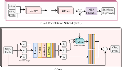
Figure 1: Graph Convolutional Network (GCN) and its building block GConv are employed in Stage 1: Generative Adversarial SG Enrichment.

-C Generator’s GCNs Architecture

The architecture of the generator’s two GCNs is the same but with different weights. First, the dimension of the data is increased to form a subspace where we can do the processing, then reduced back to a low dimension to encourage the network to extract an encoded version of input information. Finally, it returns to its original dimension. The number of neural network layers in the GCN classifiers and Enriching Edge Detector model are selected via GCN Classifier Layers and Enriching Edge Layers in Table V. In addition, at the first layers of our GCNs, two embedding linear layers without bias work as object and predicate encoders to transform the one-hot-encoded categories of objects and relationships into another continuous space.

-D CLIP Text Encoder

As the CLIP text encoder cannot handle the scene graphs directly, each edge is converted to a sentence, including the subject, the predicate, and the object of the relationship. These sentences are fed to the CLIP text encoder in addition to the objects that do not participate in any relationship as a text prompt.

Experiments

-E Image Generator

In some cases, scenes and objects synthesized with SG2IM [3] are unrecognizable even for humans, which impacts the understanding of the scene by the Stage3: Visual Evaluation & Alignment. We attempted to utilize other state-of-the-art image generators instead of SG2IM during training, such as Stable Diffusion [2], which produces $512\times 512$ and $768\times 768$ images in the most recent version. However, because of the iterative nature of their inference, generating every single image of the mini-batch without considering the backpropagation is computationally expensive. Therefore, it is impossible to get any reasonable results while doing the hyperparameter tuning in a timely manner employing more sophisticated diffusion-based high-resolution image generators.

-F Pair of Discriminators

On the VG dataset with the selected architectures, distinguishing the enriched SGs from the original data is usually far more manageable than the enrichment task. That is why our discriminators often perform far better than the generator. We tried some instances to limit the discriminator compared to the generator counterpart by having an embedded dimension selected from 16 to 256, smaller than the generator’s embedded dimension. Updating the discriminators after each generator update makes them far more powerful than their counterpart generator. That is why different settings for updating the discriminators only one time for several updates of the generator are utilized based on Update Every in Table V.

-G Training Details & Hyperparameter Tuning

HP Category	HP	Values
Batch	Size	32, 64, 128
GConv (D, G)	Dropout	0, 0.05, 0.1, 0.15, 0.25, 0.5
	Normalization	none, batch, layer
	Activation	ReLU, LeakyReLU, PReLU
Loss	Objs Weight	0.001, 0.01, 0.1, 0.5, 1, 5, 10, 50, 100, 200, 500, 1000
	Avail Preds Weight	0.001, 0.01, 0.1, 0.5, 1, 5, 10, 50, 100
	Not Avail Preds Weight	0, 0.001, 0.01, 0.1, 0.5, 1, 5, 10, 50, 100
	Edges Weight	0.001, 0.01, 0.1, 0.5, 1, 5, 10, 50, 100
	GAN Weight	0, 0.001, 0.01, 0.1, 0.5, 1, 5, 10
	Scene Features Weight	0.001, 0.01, 0.1, 0.5, 1, 5, 10, 50, 100, 200, 500, 1000
	Scene Features	logit${}_{l_{1},l_{2},CE}$, hidden${}_{l_{1},l_{2}}$, hpooled${}_{l_{1},l_{2}}$
	Image-SG Alignment Weight	1, 10, 100, 1000, 2000, 5000, 10000
Generator	Embedded Dim	16, 32, 64, 128, 256
	GCN Architecture	(a) $1\>1\>1\>1\>1$
		(b) $1\>1\>1\>1\>1\>1\>1$
		(c) $1\>4\>2\>2\>4\>1$
		(d) $1\>4\>2\>1\>1\>2\>4\>1$
		(e) $1\>4\>2\>1\>\frac{1}{2}\>\frac{1}{2}\>1\>2\>4\>1$
		(f) $1\>4\>2\>1\>\frac{1}{2}\>\frac{1}{4}\>\frac{1}{4}\>\frac{1}{2}\>1\>2\>4\>1$
	FC Dropout	0.1, 0.25, 0.5
	FC Norm	none, batch, layer
	FC Activation	ReLU, LeakyReLU, PReLU
	GCN Classifier Layers	1, 2, 4
	Enriching Edge Layers	2, 4
Discriminator	Embedded Dim	16, 32, 64, 128, 256
	GCN Architecture	(a) $1\>\frac{1}{2}\>\frac{1}{4}\>\frac{1}{8}\>\frac{1}{8}\>\frac{1}{8}$
		(b) $1\>1\>\frac{1}{2}\>\frac{1}{2}\>\frac{1}{4}\>\frac{1}{4}\>\frac{1}{8}\>\frac{1}{8}\>\frac{1}{8}$
		(c) $1\>2\>2\>1\>1\>\frac{1}{2}\>\frac{1}{2}\>\frac{1}{4}\>\frac{1}{4}\>\frac{1}{8}\>\frac{1}{8}\>\frac{1}{8}$
	Update Every	1, 5, 10, 50, 100, 200, 500, 1000, 2000

TABLE V: Hyperparameter Selections for training the network. As several loss terms are involved in the training process and considering that different values for their weights significantly impact the overall performance, we did a sweep over these options. Also, for training speed and generalizability, we tried out different options for dropout, normalization, and architecture settings. Besides, GConv HP Category is applied in both the generator and the discriminators. Also, the embedded dimension determines the data dimension after feeding the vectors to the embedding layers. In addition, the underlined values are eliminated using preliminary training only on the Generative Adversarial Scene Graph Enrichment module.

Measure/HP	SG Enrich	Deep G	Best NoD	128 BS
Objs Acc	19.04	17.31	15.09	16.85
Avail Preds Acc	41.95	39.90	40.25	31.38
Not Avail Preds Acc	-	-	3.02	-
Avail Edges Acc	75.00	75.64	76.08	66.89
Not Avail Edges Acc	99.58	99.70	99.54	99.54
Scene Class Acc	20.33	20.84	19.18	25.33
Batch Size	32	32	32	128
GConv Dropout	0.1	0.05	0.05	0
GConv Normalization	none	none	BN	none
GConv Activation	LeReLU	LeReLU	PReLU	ReLU
Objs Loss Weight	1000	500	1000	200
A Preds Loss Weight	100	50	100	50
NA Preds Loss Weight	0.1	0.01	5	0.01
Edges Loss Weight	1	0.01	100	10
GAN Loss Weight	0.1	1	0	1
Scene Features Loss Weight	200	0.1	0.001	0.01
Scene Features	$hpooled_{l_{1}}$	$logit_{l_{2}}$	$logit_{CE}$	$logit_{CE}$
G Embed Dim	256	128	128	128
G GCN Architecture	(a)	(e)	(c)	(a)
G FC Dropout	0.1	0.1	0.5	0.5
G FC Normalization	BN	none	LN	BN
G FC Activation	LeReLU	ReLU	ReLU	ReLU
G Classifier Layers	2	2	2	1
G Enriching Edge Layers	2	4	2	2
D Embed Dim	16	32	-	16
D GCN Architecture	(b)	(c)	-	(b)
D Update Every	200	1	-	1

TABLE VI: Quantitative Results, including our defined measures for the scene graph enrichment task, are exhibited for selected hyperparameter settings.

To show the iterative power of the enrichment process, the model is forced to enrich an object not already present in the input SG at each step during inference. Adam optimizer [107] is used with $10^{-4}$ as the learning rate. Also, We employed early termination for training our network based on the accuracies of the validation split. Using the proposed model on the VG dataset, continuing the training leads to improvement in training metrics and worsening validation metrics, indicating overfitting.

Table V describes the various settings used for hyperparameter tuning. Before training the model end-to-end, a hyperparameter optimization is performed, involving only our SG generator and discriminators. In other words, no image synthesizer is used at that phase. That is because training and inference time are increased while disconnecting the two mentioned components. Accordingly, the underlined values in Table V are indeed eliminated from the final hyperparameter tuning for the end-to-end model, as they performed poorly in the first stage. As already mentioned, loss weights have a crucial impact on the performance of our model. For instance, assigning a higher weight to Not Avail Preds could result in a model that outputs an enriching object without any enriching edges.

Hyperparameter tuning is performed as a sweep of different values described in Table V. Best models are picked based on a better summation of validation accuracies in the model. Among them, the ones that performed qualitatively better on a limited selection of SGs are chosen. As so many possible combinations of hyperparameters result in a huge space to discover, we select a limited combination of the parameters based on Bayes hyperparameter optimization as we train around 650 different instances.

The batch size varies from 32 to 128 scene graphs. A too-low value for batch size leads to the GPU memory and processing power not being fully utilized. A too-high value for it results in longer training time as the GT values for each SG direct the weights updates in so many different directions. This may result in a poor update at each mini-batch iteration. Dropout layers are not used in the GCN version of [3], as the authors reported that using them reduces performance. Our experiments also show the same result for higher probability values of dropout. However, we found some lower values to be beneficial for overfitting prevention. Normalization layers are not used in [3], but they potentially could aid the model to converge faster. As a result, we tried out Batch Normalization [108], Layer Normalization [109], or no normalization layer at all for our graph convolutions.

Too small values for the object loss weight or available predicates loss weight are eliminated based on our preliminary experiments, as these are two of the fundamentals of our overall objective. The option to set a weight of zero to Not Avail Preds loss is available to give the network the opportunity to update its weights based on only available predicates. In other words, when there is no edge between two objects in a scene graph, that does not mean the only possible reality is that these two do not have a relationship in a scene. Suppose the Enriching Edge Detector selects an edge where the predicate is unavailable in the GT. In that case, we may force the Enriching Predicate GCN to classify that edge as $none\_pred$, indicating no relationship based on the GT or not penalize the output predicate as the GT is indeed unavailable. This is controlled using different values for predicate loss weights.

Additionally, a zero weight option for the GAN loss is considered, resulting in no discriminator and, thus, no adversarial loss for the model. When the GT and enriched SG pair is fed to the image generator, a pair of images are synthesized, which are the inputs of the Visual Scene Characterizer. For the pair of scene features, we considered them to be selected from one of the three sources, which are the final logits affiliated with the 365 scene categories, hidden scene features before the final layer of the network, and their average pooled version. For the scene logits, three cases are considered, which are $L_{1}$ or $L_{2}$ differences and cross-entropy loss. On the other hand, for the other two scene feature types, only $L_{1}$ or $L_{2}$ differences are assessed.

The embedded dimension $D_{emb}$ for the generator is indeed the first GConv’s $D_{in}$ selected from 16 to 256. $x_{1}\>x_{2}\>...\>x_{n}$ architecture for GCN means there are $n-1$ GConv components stacked together where the $i^{th}$ GConv’s input, output, and hidden dimensions are $x_{i}D_{emb}$, $x_{i+1}D_{emb}$, and $2(x_{i}+x_{i+1})D_{emb}$, respectively.

Architectures for Discriminators’ GCNs are selected among the three available options. This architecture is, in fact, for the global discriminator, and for the local discriminator, the last two graph convolution layers are eliminated to have a shallower version.

(a) Input Scene Graph

(b) Enriched Scene Graph

(c) Input/Enriched Text

(d) Simple Image

(e) Enriched Image

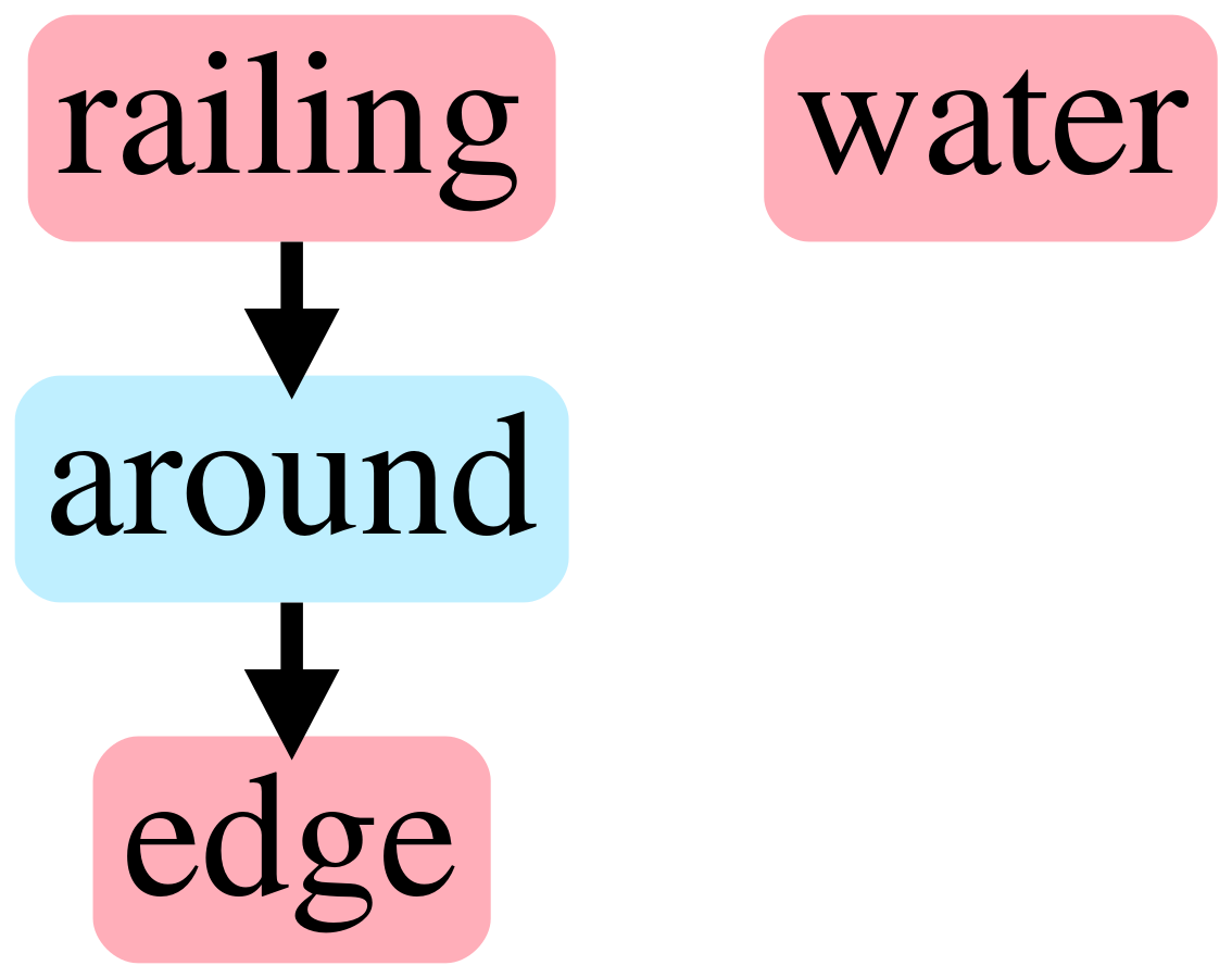
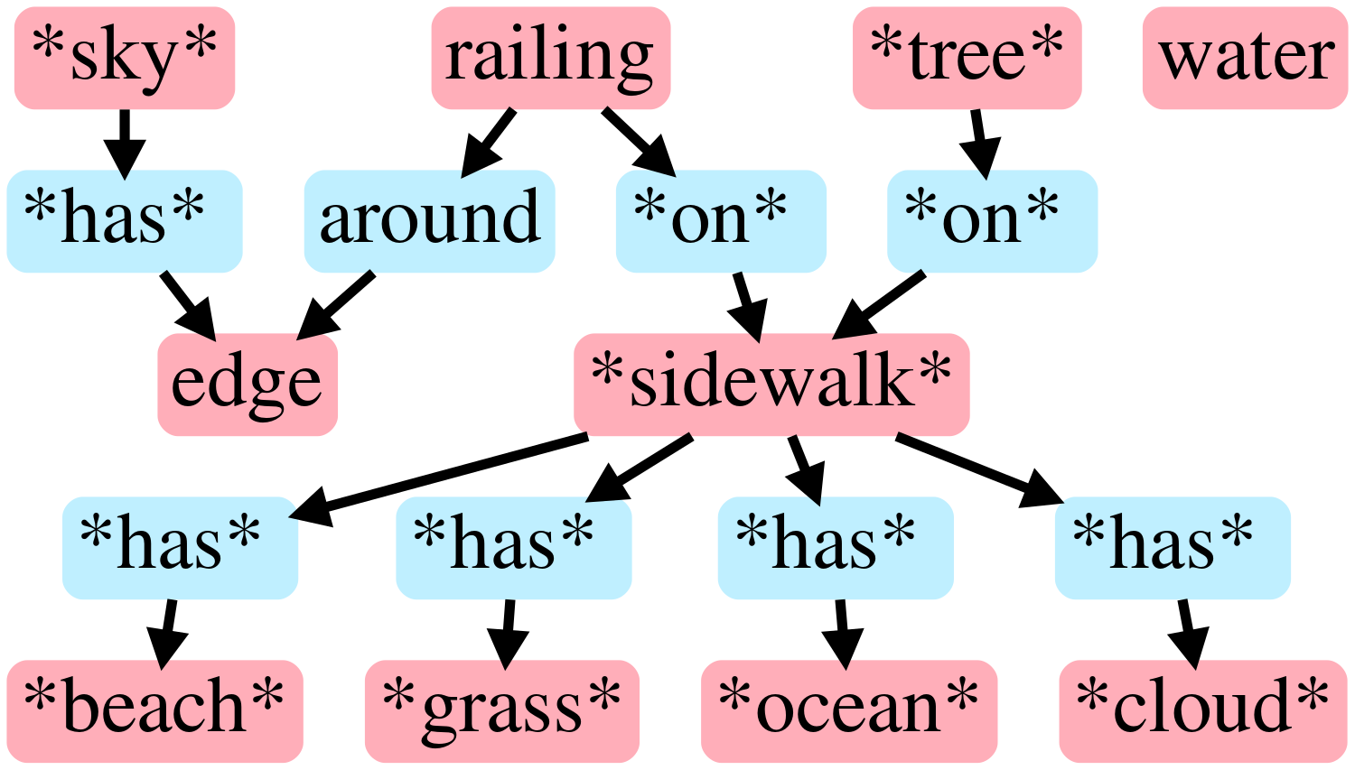
Railing on sidewalk and around edge. Water. Sky has edge. Tree on sidewalk that has beach, ocean, grass, and cloud.
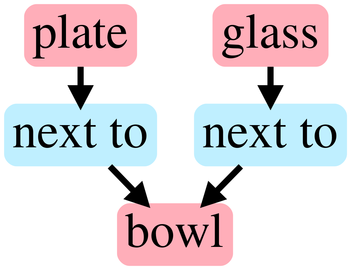
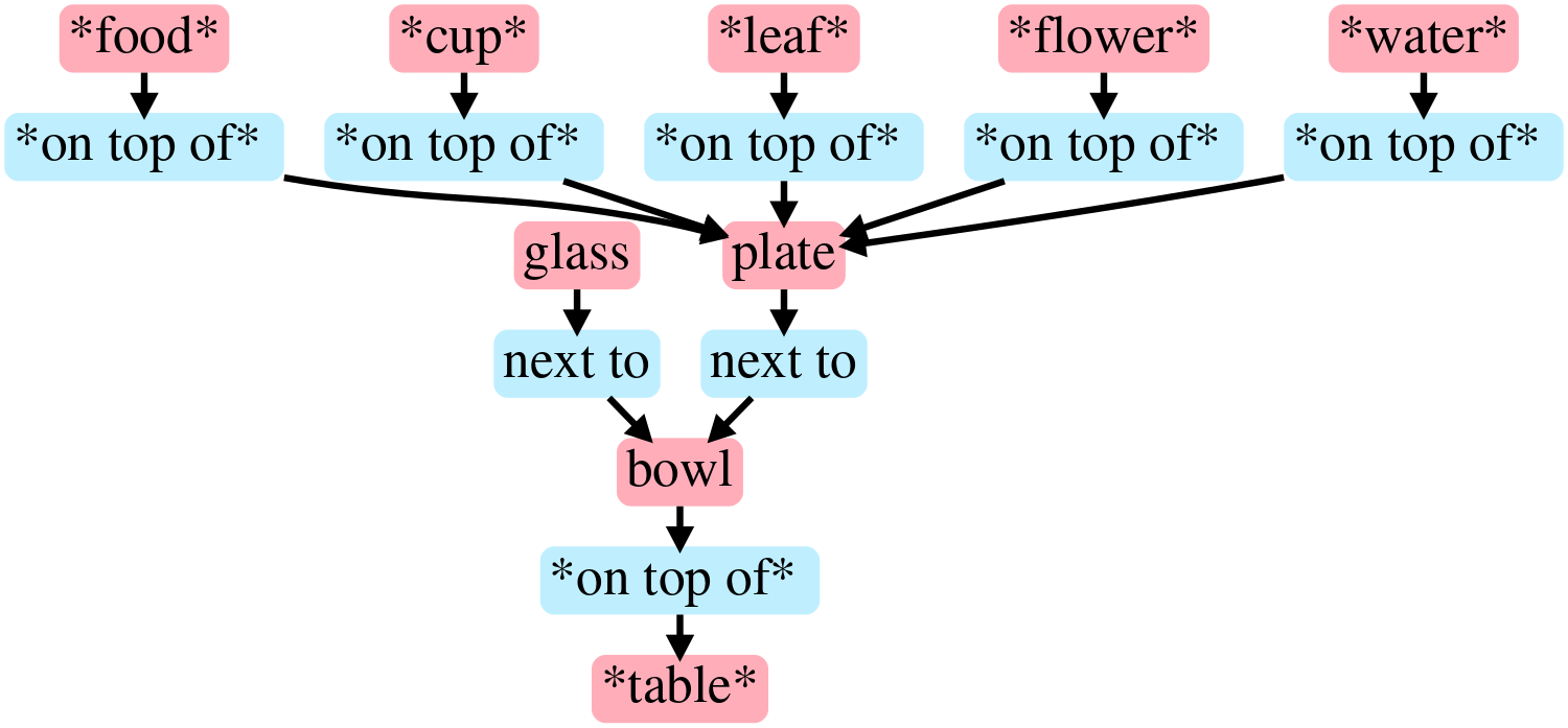
Plate and glass next to bowl on top of table. Food, cup, leaf, flower, water on top of plate.
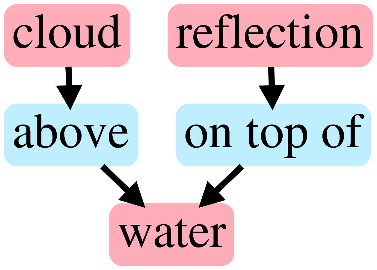
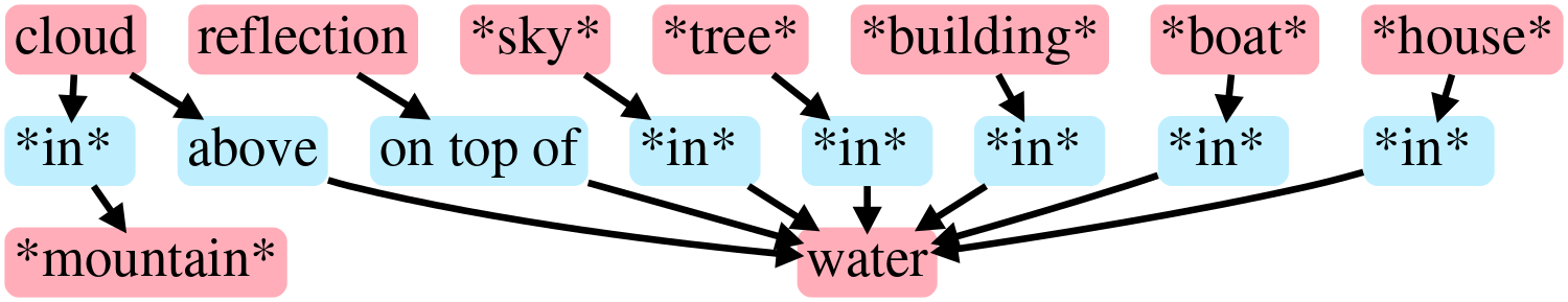
Cloud in mountain. Cloud above water. Reflection on top of water. Sky, tree, building, boat, and house in water.
Glass with water on table. Plate with pizza. Cup, handle, bottle, food, bowl, glasses, and hand on table.
Snow on top of truck next to road. Sky, tree, sign, line, ground, building, car, cloud, and sidewalk on road.
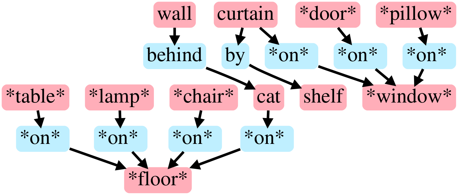
Wall behind cat on floor. Chair, lamp, and table on floor. Curtain by shelf. Curtain on window. Pillow on window. Door on window.
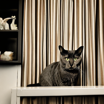
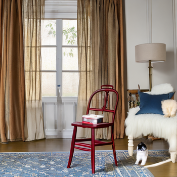
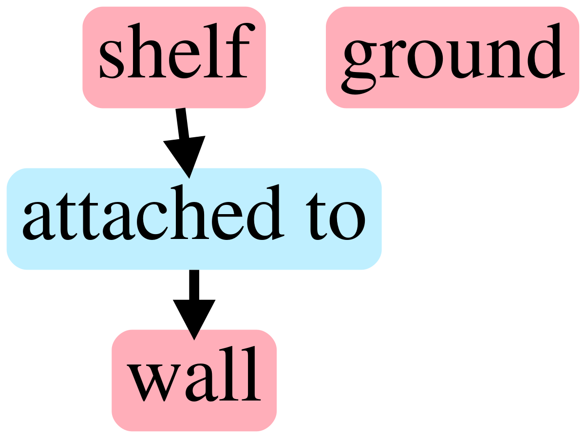
Book on shelf attached to wall. Ground. Paper attached to wall.

Figure 3: Qualitative Results. Samples of Visual Genome scene graphs and their enriched descriptions along with their corresponding synthesized images.

(a) Input Scene Graph

(b) Enriched Scene Graph

(c) Input/Enriched Text

(d) Simple Image

(e) Enriched Image

Car. Sign on road near street. Bus and line on street near tree and building. Sky and sidewalk near building.
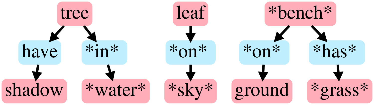
Tree has shadow. Tree in water. Leaf on sky. Bench on ground. Bench has grass.
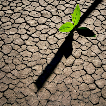
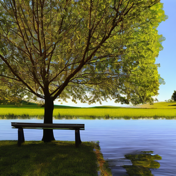
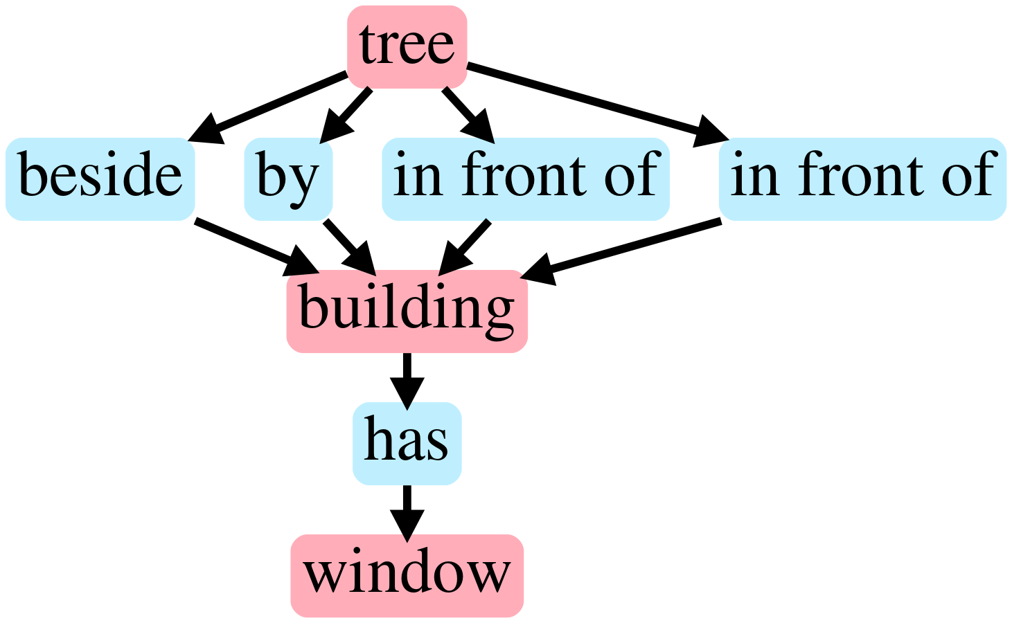
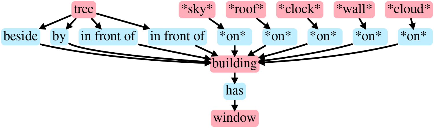
Tree in front of and beside building that has window. Clock on building. Sky, roof, wall and cloud on building.
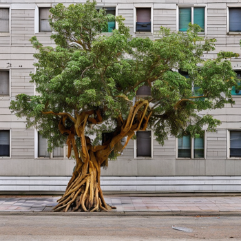
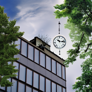
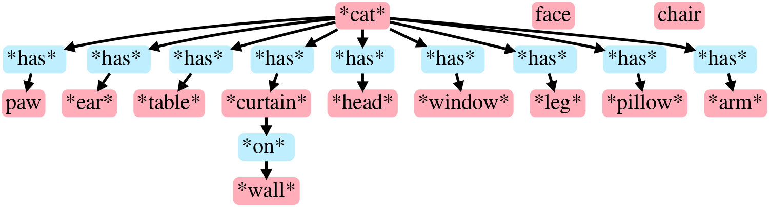
Cat has paw, ear, head, leg and arm. Cat has table, window and pillow. Cat has Curtain on wall. Chair and Face.
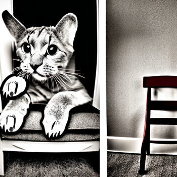
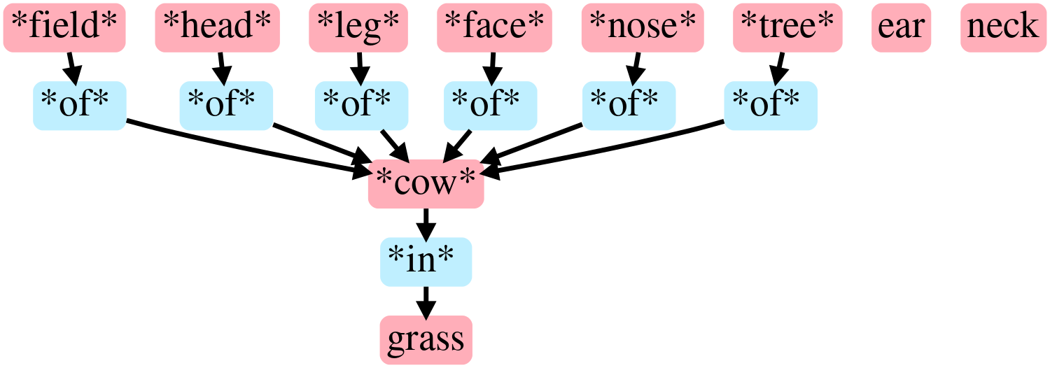
Field of cow in grass. Head, leg, face, and nose of cow. Tree of cow. Ear and neck.
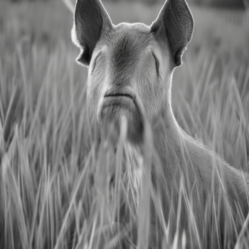
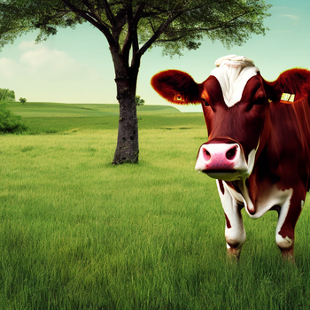
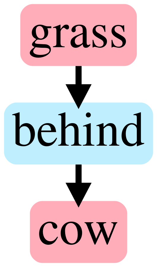
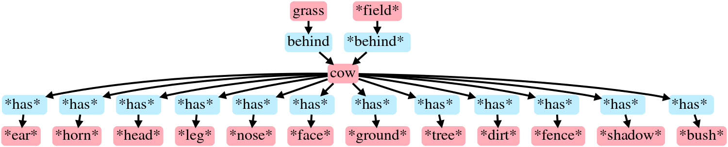
Grass and field behind cow. Cow has ear, horn, head, leg, nose, and face. Cow has bush, shadow, fence, dirt, tree, and ground.
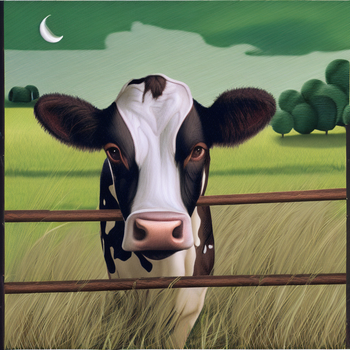
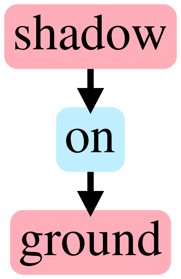
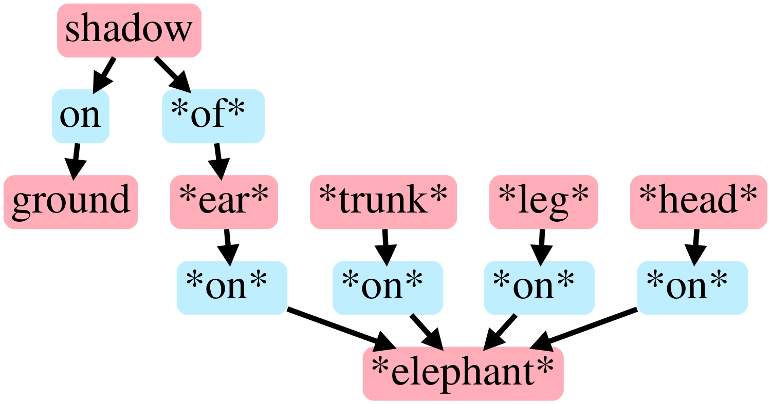
Shadow of ear on ground. Ear, trunk, leg, and head on elephant.

Figure 4: Qualitative Results, similar to Fig. 3

References

- [1] R. Krishna, Y. Zhu, O. Groth, J. Johnson, K. Hata, J. Kravitz, S. Chen, Y. Kalantidis, L.-J. Li, D. A. Shamma et al., “Visual genome: Connecting language and vision using crowdsourced dense image annotations,” International journal of computer vision, vol. 123, pp. 32–73, 2017.
- [2] R. Rombach, A. Blattmann, D. Lorenz, P. Esser, and B. Ommer, “High-resolution image synthesis with latent diffusion models,” in Proceedings of the IEEE/CVF Conference on Computer Vision and Pattern Recognition, 2022, pp. 10 684–10 695.
- [3] J. Johnson, A. Gupta, and L. Fei-Fei, “Image generation from scene graphs,” in Proceedings of the IEEE conference on computer vision and pattern recognition, 2018, pp. 1219–1228.
- [4] I. Goodfellow, J. Pouget-Abadie, M. Mirza, B. Xu, D. Warde-Farley, S. Ozair, A. Courville, and Y. Bengio, “Generative adversarial networks,” Communications of the ACM, vol. 63, no. 11, pp. 139–144, 2020.
- [5] A. Radford, L. Metz, and S. Chintala, “Unsupervised representation learning with deep convolutional generative adversarial networks,” arXiv preprint arXiv:1511.06434, 2015.
- [6] A. Brock, J. Donahue, and K. Simonyan, “Large scale gan training for high fidelity natural image synthesis,” arXiv preprint arXiv:1809.11096, 2018.
- [7] T. Karras, S. Laine, M. Aittala, J. Hellsten, J. Lehtinen, and T. Aila, “Analyzing and improving the image quality of stylegan,” in Proceedings of the IEEE/CVF conference on computer vision and pattern recognition, 2020, pp. 8110–8119.
- [8] M. Mirza and S. Osindero, “Conditional generative adversarial nets,” arXiv preprint arXiv:1411.1784, 2014.
- [9] A. Odena, C. Olah, and J. Shlens, “Conditional image synthesis with auxiliary classifier gans,” in International conference on machine learning. PMLR, 2017, pp. 2642–2651.
- [10] L. Metz, B. Poole, D. Pfau, and J. Sohl-Dickstein, “Unrolled generative adversarial networks,” arXiv preprint arXiv:1611.02163, 2016.
- [11] S. Reed, Z. Akata, X. Yan, L. Logeswaran, B. Schiele, and H. Lee, “Generative adversarial text to image synthesis,” in International conference on machine learning. PMLR, 2016, pp. 1060–1069.
- [12] S. E. Reed, Z. Akata, S. Mohan, S. Tenka, B. Schiele, and H. Lee, “Learning what and where to draw,” Advances in neural information processing systems, vol. 29, 2016.
- [13] H. Zhang, T. Xu, H. Li, S. Zhang, X. Wang, X. Huang, and D. N. Metaxas, “Stackgan++: Realistic image synthesis with stacked generative adversarial networks,” IEEE transactions on pattern analysis and machine intelligence, vol. 41, no. 8, pp. 1947–1962, 2018.
- [14] T. Xu, P. Zhang, Q. Huang, H. Zhang, Z. Gan, X. Huang, and X. He, “Attngan: Fine-grained text to image generation with attentional generative adversarial networks,” in Proceedings of the IEEE conference on computer vision and pattern recognition, 2018, pp. 1316–1324.
- [15] D. Bahdanau, K. Cho, and Y. Bengio, “Neural machine translation by jointly learning to align and translate,” arXiv preprint arXiv:1409.0473, 2014.
- [16] A. Vaswani, N. Shazeer, N. Parmar, J. Uszkoreit, L. Jones, A. N. Gomez, Ł. Kaiser, and I. Polosukhin, “Attention is all you need,” Advances in neural information processing systems, vol. 30, 2017.
- [17] D. P. Kingma and M. Welling, “Auto-encoding variational bayes,” arXiv preprint arXiv:1312.6114, 2013.
- [18] A. Vahdat and J. Kautz, “Nvae: A deep hierarchical variational autoencoder,” Advances in neural information processing systems, vol. 33, pp. 19 667–19 679, 2020.
- [19] H. Huang, R. He, Z. Sun, T. Tan et al., “Introvae: Introspective variational autoencoders for photographic image synthesis,” Advances in neural information processing systems, vol. 31, 2018.
- [20] A. Van Den Oord, N. Kalchbrenner, and K. Kavukcuoglu, “Pixel recurrent neural networks,” in International conference on machine learning. PMLR, 2016, pp. 1747–1756.
- [21] A. Van den Oord, N. Kalchbrenner, L. Espeholt, O. Vinyals, A. Graves et al., “Conditional image generation with pixelcnn decoders,” Advances in neural information processing systems, vol. 29, 2016.
- [22] M. Chen, A. Radford, R. Child, J. Wu, H. Jun, D. Luan, and I. Sutskever, “Generative pretraining from pixels,” in International conference on machine learning. PMLR, 2020, pp. 1691–1703.
- [23] R. Child, S. Gray, A. Radford, and I. Sutskever, “Generating long sequences with sparse transformers,” arXiv preprint arXiv:1904.10509, 2019.
- [24] J. Yu, Y. Xu, J. Y. Koh, T. Luong, G. Baid, Z. Wang, V. Vasudevan, A. Ku, Y. Yang, B. K. Ayan et al., “Scaling autoregressive models for content-rich text-to-image generation,” arXiv preprint arXiv:2206.10789, 2022.
- [25] J. Sohl-Dickstein, E. Weiss, N. Maheswaranathan, and S. Ganguli, “Deep unsupervised learning using nonequilibrium thermodynamics,” in International Conference on Machine Learning. PMLR, 2015, pp. 2256–2265.
- [26] P. Dhariwal and A. Nichol, “Diffusion models beat gans on image synthesis,” Advances in Neural Information Processing Systems, vol. 34, pp. 8780–8794, 2021.
- [27] J. Ho, A. Jain, and P. Abbeel, “Denoising diffusion probabilistic models,” Advances in Neural Information Processing Systems, vol. 33, pp. 6840–6851, 2020.
- [28] Y. Song, J. Sohl-Dickstein, D. P. Kingma, A. Kumar, S. Ermon, and B. Poole, “Score-based generative modeling through stochastic differential equations,” arXiv preprint arXiv:2011.13456, 2020.
- [29] C. Saharia, W. Chan, S. Saxena, L. Li, J. Whang, E. Denton, S. K. S. Ghasemipour, B. K. Ayan, S. S. Mahdavi, R. G. Lopes et al., “Photorealistic text-to-image diffusion models with deep language understanding,” arXiv preprint arXiv:2205.11487, 2022.
- [30] A. Razavi, A. Van den Oord, and O. Vinyals, “Generating diverse high-fidelity images with vq-vae-2,” Advances in neural information processing systems, vol. 32, 2019.
- [31] W. Yan, Y. Zhang, P. Abbeel, and A. Srinivas, “Videogpt: Video generation using vq-vae and transformers,” arXiv preprint arXiv:2104.10157, 2021.
- [32] P. Esser, R. Rombach, and B. Ommer, “Taming transformers for high-resolution image synthesis,” in Proceedings of the IEEE/CVF conference on computer vision and pattern recognition, 2021, pp. 12 873–12 883.
- [33] J. Yu, X. Li, J. Y. Koh, H. Zhang, R. Pang, J. Qin, A. Ku, Y. Xu, J. Baldridge, and Y. Wu, “Vector-quantized image modeling with improved vqgan,” arXiv preprint arXiv:2110.04627, 2021.
- [34] A. Sperduti and A. Starita, “Supervised neural networks for the classification of structures,” IEEE Trans. Neural Netw., vol. 8, no. 3, pp. 714–735, May 1997.
- [35] M. Gori, G. Monfardini, and F. Scarselli, “A new model for learning in graph domains,” in Proc. IEEE Int, J. Conf, Ed. vol. 2: Neural Netw, August 2005, pp. 729–734.
- [36] F. Scarselli, M. Gori, A. C. Tsoi, M. Hagenbuchner, and G. Monfardini, “The graph neural network model,” IEEE Trans. Neural Netw., vol. 20, no. 1, pp. 61–80, January 2009.
- [37] T. N. Kipf and M. Welling, “Semi-supervised classification with graph convolutional networks,” arXiv preprint arXiv:1609.02907, 2016.
- [38] P. Veličković, G. Cucurull, A. Casanova, A. Romero, P. Lio, and Y. Bengio, “Graph attention networks,” arXiv preprint arXiv:1710.10903, 2017.
- [39] J. Bruna, W. Zaremba, A. Szlam, and Y. LeCun, “Spectral networks and locally connected networks on graphs,” in Proc. ICLR, 2014, pp. 1–14.
- [40] M. Henaff, J. Bruna, and Y. LeCun, Deep convolutional networks on graph-structured data, [Online]. Available, 2015. [Online]. Available: http://arxiv.org/abs/1506.05163
- [41] M. Defferrard, X. Bresson, and P. V. der Gheynst, “Convolutional neural networks on graphs with fast localized spectral filtering,” in Proc. NIPS, 2016, pp. 3844–3852.
- [42] R. Levie, F. Monti, X. Bresson, and M. M. Bronstein, “Cayleynets: Graph convolutional neural networks with complex rational spectral filters,” IEEE Trans. Signal Process, vol. 67, no. 1, pp. 97–109, January 2019.
- [43] A. Micheli, “Neural network for graphs: A contextual constructive approach,” IEEE Trans. Neural Netw., vol. 20, no. 3, pp. 498–511, March 2009.
- [44] J. Atwood and D. Towsley, “Diffusion-convolutional neural networks,” in Proc. NIPS, 2016, pp. 1993–2001.
- [45] M. Niepert, M. Ahmed, and K. Kutzkov, “Learning convolutional neural networks for graphs,” in Proc. 33rd Int. Conf. Mach. Learn, 2016, pp. 2014–2023.
- [46] J. Gilmer, S. S. Schoenholz, P. F. Riley, O. Vinyals, and G. E. Dahl, “Neural message passing for quantum chemistry,” in Proc. 34th Int. Conf. Mach. Learn, 2017, pp. 1263–1272.
- [47] Z. Wu, S. Pan, F. Chen, G. Long, C. Zhang, and S. Y. Philip, “A comprehensive survey on graph neural networks,” IEEE transactions on neural networks and learning systems, vol. 32, no. 1, pp. 4–24, 2020.
- [48] C. Wang, S. Pan, G. Long, X. Zhu, and J. Jiang, “Mgae: Marginalized graph autoencoder for graph clustering,” in Proc. CIKM, 2017, pp. 889–898.
- [49] T. Kawamoto, M. Tsubaki, and T. Obuchi, “Mean-field theory of graph neural networks in graph partitioning,” in Proc. NeurIPS, 2018, pp. 4362–4372.
- [50] D. Marcheggiani and I. Titov, “Encoding sentences with graph convolutional networks for semantic role labeling,” in Proc. Conf. Empirical Methods Natural Lang. Process, 2017, pp. 1506–1515.
- [51] D. Marcheggiani, J. Bastings, and I. Titov, “Exploiting semantics in neural machine translation with graph convolutional networks,” in Proc. NAACL, 2018, pp. 1–8.
- [52] J. Bastings, I. Titov, W. Aziz, D. Marcheggiani, and K. Simaan, “Graph convolutional encoders for syntax-aware neural machine translation,” in Proc. Conf. Empirical Methods Natural Lang. Process, 2017, pp. 1957–1967.
- [53] R. van den Berg, T. N. Kipf, and M. Welling, Graph convolutional matrix completion, [Online]. Available, 2017. [Online]. Available: https://arxiv.org/abs/1706.02263
- [54] R. Ying, R. He, K. Chen, P. Eksombatchai, W. L. Hamilton, and J. Leskovec, “Graph convolutional neural networks for web-scale recommender systems,” in Proc. 24th ACM SIGKDD Int. Conf. Knowl. Discovery Data Mining, August 2018, pp. 974–983.
- [55] Y. Li, D. Tarlow, M. Brockschmidt, and R. Zemel, “Gated graph sequence neural networks,” in Proc. ICLR, 2015, pp. 1–20.
- [56] M. Allamanis, M. Brockschmidt, and M. Khademi, “Learning to represent programs with graphs,” in Proc. ICLR, 2017, pp. 1–17.
- [57] J. Qiu, J. Tang, H. Ma, Y. Dong, K. Wang, and J. Tang, “Deepinf: Social influence prediction with deep learning,” in Proc. KDD, 2018, pp. 2110–2119.
- [58] D. Zugner, A. Akbarnejad, and S. Gunnemann, “Adversarial attacks on neural networks for graph data,” in Proc. 24th ACM SIGKDD Int. Conf. Knowl. Discovery Data Mining (KDD), August 2019, pp. 2847–2856.
- [59] J. K. al., “Brainnetcnn: Convolutional neural networks for brain networks; towards predicting neurodevelopment,” NeuroImage, vol. 146, pp. 1038–1049, February 2017.
- [60] Z. Li, Q. Chen, and V. Koltun, “Combinatorial optimization with graph convolutional networks and guided tree search,” in Proc. NeurIPS, 2018, pp. 536–545.
- [61] T. H. Nguyen and R. Grishman, “Graph convolutional networks with argument-aware pooling for event detection,” in Proc. AAAI, 2018, pp. 5900–5907.
- [62] D. K. D. al., “Convolutional networks on graphs for learning molecular fingerprints,” in Proc. NIPS, 2015, pp. 2224–2232.
- [63] Y. Li, O. Vinyals, C. Dyer, R. Pascanu, and P. Battaglia, “Learning deep generative models of graphs,” in Proc. ICML, 2018, pp. 1–21.
- [64] J. You, B. Liu, R. Ying, V. Pande, and J. Leskovec, “Graph convolutional policy network for goal-directed molecular graph generation,” in Proc. NeurIPS, 2018, pp. 6410–6421.
- [65] H. Y. al., “Deep multi-view spatial-temporal network for taxi demand prediction,” in Proc. AAAI, 2018, pp. 2588–2595.
- [66] A. Jain, A. R. Zamir, S. Savarese, and A. Saxena, “Structural-rnn: Deep learning on spatio-temporal graphs,” in Proc. IEEE Conf. Comput. Vis. Pattern Recognit. (CVPR), June 2016, pp. 5308–5317.
- [67] S. Yan, Y. Xiong, and D. Lin, “Spatial temporal graph convolutional networks for skeleton-based action recognition,” in Proc. AAAI, 2018, pp. 1–9.
- [68] Y. Wang, Y. Sun, Z. Liu, S. E. Sarma, M. M. Bronstein, and J. M. Solomon, “Dynamic graph cnn for learning on point clouds,” ACM Trans. Graph, vol. 38, no. 5, pp. 1–12, October 2019.
- [69] L. Landrieu and M. Simonovsky, “Large-scale point cloud semantic segmentation with superpoint graphs,” in Proc. IEEE/CVF Conf. Comput. Vis. Pattern Recognit, June 2018, pp. 4558–4567.
- [70] S. Qi, W. Wang, B. Jia, J. Shen, and S.-C. Zhu, “Learning humanobject interactions by graph parsing neural networks,” in Proc. Eur. Conf. Comput. Vis, 2018, pp. 407–423.
- [71] V. G. Satorras and J. B. Estrach, “Few-shot learning with graph neural networks,” in Proc. ICLR, 2018, pp. 1–13.
- [72] M. Narasimhan, S. Lazebnik, and A. Schwing, “Out of the box: Reasoning with graph convolution nets for factual visual question answering,” in Proc. NeurIPS, 2018, pp. 2655–2666.
- [73] X. Chen, L.-J. Li, L. Fei-Fei, and A. Gupta, “Iterative visual reasoning beyond convolutions,” in Proc. IEEE/CVF Conf. Comput. Vis. Pattern Recognit, 2018, pp. 7239–7248.
- [74] L. Yi, H. Su, X. Guo, and L. Guibas, “Syncspeccnn: Synchronized spectral cnn for 3d shape segmentation,” in Proc. IEEE Conf. Comput. Vis. Pattern Recognit. (CVPR), July 2017, pp. 6584–6592.
- [75] J. J. al., “Image retrieval using scene graphs,” in Proc. IEEE Conf. Comput. Vis. Pattern Recognit, 2015, pp. 3668–3678.
- [76] S. Tripathi, K. Nguyen, T. Guha, B. Du, and T. Q. Nguyen, “Sg2caps: Revisiting scene graphs for image captioning,” 2021.
- [77] A. R. al., “Kimera: From slam to spatial perception with 3d dynamic scene graphs,” 2021.
- [78] J. Zhang, K. J. Shih, A. Elgammal, A. Tao, and B. Catanzaro, “Graphical contrastive losses for scene graph generation,” 2019.
- [79] X. Chang, P. Ren, P. Xu, Z. Li, X. Chen, and A. Hauptmann, “A comprehensive survey of scene graphs: Generation and application,” IEEE Transactions on Pattern Analysis and Machine Intelligence, vol. 45, no. 1, pp. 1–26, 2021.
- [80] E. E. Aksoy, A. Abramov, F. Wo€rgo€tter, and B. Dellen, “Categorizing object-action relations from semantic scene graphs,” in Proc. IEEE Int. Conf. Robot. Autom, 2010, pp. 398–405.
- [81] S. Aditya, Y. Yang, C. Baral, C. Fermuller, and Y. Aloimonos, “From images to sentences through scene description graphs using commonsense reasoning and knowledge,” 2015.
- [82] J. Johnson, R. Krishna, M. Stark, L.-J. Li, D. Shamma, M. Bernstein, and L. Fei-Fei, “Image retrieval using scene graphs,” in Proceedings of the IEEE conference on computer vision and pattern recognition, 2015, pp. 3668–3678.
- [83] C. Lu, R. Krishna, M. Bernstein, and L. Fei-Fei, “Visual relationship detection with language priors,” in Computer Vision–ECCV 2016: 14th European Conference, Amsterdam, The Netherlands, October 11–14, 2016, Proceedings, Part I 14. Springer, 2016, pp. 852–869.
- [84] D. Xu, Y. Zhu, C. B. Choy, and L. Fei-Fei, “Scene graph generation by iterative message passing,” in Proceedings of the IEEE conference on computer vision and pattern recognition, 2017, pp. 5410–5419.
- [85] J. Yang, J. Lu, S. Lee, D. Batra, and D. Parikh, “Graph r-cnn for scene graph generation,” in Proceedings of the European conference on computer vision (ECCV), 2018, pp. 670–685.
- [86] K. Tang, Y. Niu, J. Huang, J. Shi, and H. Zhang, “Unbiased scene graph generation from biased training,” in Proceedings of the IEEE/CVF conference on computer vision and pattern recognition, 2020, pp. 3716–3725.
- [87] J. Yang, Y. Z. Ang, Z. Guo, K. Zhou, W. Zhang, and Z. Liu, “Panoptic scene graph generation,” in Computer Vision–ECCV 2022: 17th European Conference, Tel Aviv, Israel, October 23–27, 2022, Proceedings, Part XXVII. Springer, 2022, pp. 178–196.
- [88] Y. Li, W. Ouyang, B. Zhou, J. Shi, C. Zhang, and X. Wang, “Factorizable net: An efficient subgraph-based framework for scene graph generation,” in Proc. Eur. Conf. Comput. Vis, 2018, pp. 346–363.
- [89] L. Yang, Z. Huang, Y. Song, S. Hong, G. Li, W. Zhang, B. Cui, B. Ghanem, and M.-H. Yang, “Diffusion-based scene graph to image generation with masked contrastive pre-training,” arXiv preprint arXiv:2211.11138, 2022.
- [90] R. Herzig, A. Bar, H. Xu, G. Chechik, T. Darrell, and A. Globerson, “Learning canonical representations for scene graph to image generation,” in Computer Vision–ECCV 2020: 16th European Conference, Glasgow, UK, August 23–28, 2020, Proceedings, Part XXVI 16. Springer, 2020, pp. 210–227.
- [91] Y. Li, T. Ma, Y. Bai, N. Duan, S. Wei, and X. Wang, “Pastegan: A semi-parametric method to generate image from scene graph,” Advances in Neural Information Processing Systems, vol. 32, 2019.
- [92] O. Ashual and L. Wolf, “Specifying object attributes and relations in interactive scene generation,” in Proceedings of the IEEE/CVF international conference on computer vision, 2019, pp. 4561–4569.
- [93] C.-A. Yang, C.-Y. Tan, W.-C. Fan, C.-F. Yang, M.-L. Wu, and Y.-C. F. Wang, “Scene graph expansion for semantics-guided image outpainting,” in Proceedings of the IEEE/CVF Conference on Computer Vision and Pattern Recognition, 2022, pp. 15 617–15 626.
- [94] S. Iizuka, E. Simo-Serra, and H. Ishikawa, “Globally and locally consistent image completion,” ACM Transactions on Graphics (ToG), vol. 36, no. 4, pp. 1–14, 2017.
- [95] B. Zhou, A. Lapedriza, A. Khosla, A. Oliva, and A. Torralba, “Places: A 10 million image database for scene recognition,” IEEE transactions on pattern analysis and machine intelligence, vol. 40, no. 6, pp. 1452–1464, 2017.
- [96] A. Radford, J. W. Kim, C. Hallacy, A. Ramesh, G. Goh, S. Agarwal, G. Sastry, A. Askell, P. Mishkin, J. Clark et al., “Learning transferable visual models from natural language supervision,” in International conference on machine learning. PMLR, 2021, pp. 8748–8763.
- [97] T. Brown, B. Mann, N. Ryder, M. Subbiah, J. D. Kaplan, P. Dhariwal, A. Neelakantan, P. Shyam, G. Sastry, A. Askell et al., “Language models are few-shot learners,” Advances in neural information processing systems, vol. 33, pp. 1877–1901, 2020.
- [98] OpenAI, “Gpt-4 technical report,” 2023.
- [99] H. Touvron, L. Martin, K. Stone, P. Albert, A. Almahairi, Y. Babaei, N. Bashlykov, S. Batra, P. Bhargava, S. Bhosale et al., “Llama 2: Open foundation and fine-tuned chat models,” arXiv preprint arXiv:2307.09288, 2023.
- [100] T. L. Scao, A. Fan, C. Akiki, E. Pavlick, S. Ilić, D. Hesslow, R. Castagné, A. S. Luccioni, F. Yvon, M. Gallé et al., “Bloom: A 176b-parameter open-access multilingual language model,” arXiv preprint arXiv:2211.05100, 2022.
- [101] L. Ouyang, J. Wu, X. Jiang, D. Almeida, C. Wainwright, P. Mishkin, C. Zhang, S. Agarwal, K. Slama, A. Ray et al., “Training language models to follow instructions with human feedback,” Advances in Neural Information Processing Systems, vol. 35, pp. 27 730–27 744, 2022.
- [102] R. Anil, A. M. Dai, O. Firat, M. Johnson, D. Lepikhin, A. Passos, S. Shakeri, E. Taropa, P. Bailey, Z. Chen et al., “Palm 2 technical report,” arXiv preprint arXiv:2305.10403, 2023.
- [103] D. Driess, F. Xia, M. S. Sajjadi, C. Lynch, A. Chowdhery, B. Ichter, A. Wahid, J. Tompson, Q. Vuong, T. Yu et al., “Palm-e: An embodied multimodal language model,” arXiv preprint arXiv:2303.03378, 2023.
- [104] T. Salimans, I. Goodfellow, W. Zaremba, V. Cheung, A. Radford, and X. Chen, “Improved techniques for training gans,” Advances in neural information processing systems, vol. 29, 2016.
- [105] M. Heusel, H. Ramsauer, T. Unterthiner, B. Nessler, and S. Hochreiter, “Gans trained by a two time-scale update rule converge to a local nash equilibrium,” Advances in neural information processing systems, vol. 30, 2017.
- [106] T.-Y. Lin, M. Maire, S. Belongie, J. Hays, P. Perona, D. Ramanan, P. Dollár, and C. L. Zitnick, “Microsoft coco: Common objects in context,” in Computer Vision–ECCV 2014: 13th European Conference, Zurich, Switzerland, September 6-12, 2014, Proceedings, Part V 13. Springer, 2014, pp. 740–755.
- [107] D. P. Kingma and J. Ba, “Adam: A method for stochastic optimization,” arXiv preprint arXiv:1412.6980, 2014.
- [108] S. Ioffe and C. Szegedy, “Batch normalization: Accelerating deep network training by reducing internal covariate shift,” in International conference on machine learning. pmlr, 2015, pp. 448–456.
- [109] J. L. Ba, J. R. Kiros, and G. E. Hinton, “Layer normalization,” arXiv preprint arXiv:1607.06450, 2016.