Entanglement in selected Binary Tree States: Dicke/Total spin states, particle number projected BCS states

Abstract

Binary Tree States (BTS) are states whose decomposition on a quantum register basis formed by a set of qubits can be made sequentially. Such states sometimes appear naturally in many-body systems treated in Fock space when a global symmetry is imposed, like the total spin or particle number symmetries. Examples are the Dicke states, the eigenstates of the total spin for a set of particles having individual spin $1/2$, or states obtained by projecting a BCS states onto particle number, also called projected BCS in small superfluid systems. Starting from a BTS state described on the set of $n$ qubits or orbitals, the entanglement entropy of any subset of $k$ qubits is analyzed. Specifically, a practical method is developed to access the $k$ qubits/particles von Neumann entanglement entropy of the subsystem of interest. Properties of these entropies are discussed, including scaling properties, upper bounds, or how these entropies correlate with fluctuations. Illustrations are given for the Dicke state and the projected BCS states.

I Introduction

With the progress in quantum computing McC16 ; Cao19 ; McA20 ; Bau21 ; Bha21 ; End21 ; Ayr23 or in novel techniques to treat many-body systems, like tensor networks Cir21 , the understanding of entanglement in interacting systems found in physics or chemistry is attracting more attention. In recent years, several attempts have been made to better characterize quantum entanglement in nuclear physics Rob21 ; Joh23 ; Paz23 ; Bul23 ; Bul23-b ; Per23 . Among the current discussions on the subject, one can mention the important role of spontaneous symmetry breaking Fab21 ; Fab22 that might be connected to a quantum phase transition or might characterize correlations in many-body systems Dus04 ; Vid04a ; Vid04b ; Vid04c ; Dit19 , or the ”volume/area law” nature of entanglement Gu23 . quantifying entanglement might also be very useful in practice for improving the convergence of many-body theories, as was firstly shown in quantum chemistry Ste16 ; Ste19 and more recently analyzed in nuclear physics Mom23 ; Tic23 . The possible measure of entanglement through the study of fluctuations in nuclear reactions has also been discussed very recently Li24 .

Most of the studies so far aim to study the one particle or, eventually, two particles entanglement using a variety of tools, like the von-Neumann reduced entropy, Renyi entropy, and mutual information Nie00 ; Ami08 ; Hor09 ; Laf16 ; Sri24 … In this work, I point out that, due to some specificities of some of the states used in many-body systems, one can access more generally their $k$-particles entropy. Specifically, I use the fact that symmetries affect entanglement by creating block structures in reduced-density matrices. As an illustration, in Ref. Lac22 , we have empirically shown that the entanglement entropy of $k$ interacting neutrinos with $k>1$ acquires a rather simple scaling property compared to the one neutrino entropy. Such a scaling can be partially understood from the permutation invariance of the problem. This finding was one of the motivations for the present work.

In this work, I consider a certain class of states relevant to the symmetry problem in fields like quantum chemistry when total spin is conserved or in nuclear physics when treating superfluity using projected quasi-particle states. Following Ref. Kha23 ; Dut23 , where a quantum computer algorithm is proposed to build such states, they will be called here generically Binary-Tree-State (BTS). BTS states include the Dicke states Dic54 , the total spin eigenstates in systems formed of particles with spin Mes62 ; Low69 , and, as we will see, the so-called projected BCS states (BCS states) Rin80 ; Bla86 ; Del01 ; Bri05 . The entanglement properties of the Dicke state are rather well-known and will serve as a guide for other BTS states below. Still, a study of the general entanglement properties of projected quasi-particle states has yet to be made.

The present discussion is relevant for many-body systems but can have some interest in the context of quantum computing. For this reason, my starting point will be to consider a set of two-level systems, with levels labeled $0$ and $1$, that will be called hereafter generically qubits. When working with a set of particles with spins $1/2$, each of the two levels will represent the two possible spins of the particle. When considering a many-body problem, each two-level is assigned to a single particle orbital treated in Fock space, and its occupation is assigned to the level $1$ while its vacancy is assigned to $0$.

The article is organized as follows. First, BTS states are introduced, and a method to evaluate the entanglement of any bipartition of the system is developed. Then, two illustrative cases are considered: the fully permutation invariant Dicke state and the projected BCS state. Special attention is paid to the entanglement entropy’s scaling properties and upper limits.

II Binary Tree States

I consider here a set of $n$ qubits labelled by $i=1,\cdots,n$, where each qubit can access two states $\{|0_{i}\rangle,|1_{i}\rangle\}$, and I denote below $\{X_{i},Y_{i},Z_{i}\}$ the corresponding Pauli matrices. Connection with many-body systems described in Fock space can be made through the Jordan-Wigner transformation Jor28 ; Lie61 giving a mapping between the occupation or not of single-orbital with the occupation of the $|1_{i}\rangle$ and $|0_{i}\rangle$ state, respectively. A state $|\Psi\rangle$ can be decomposed in the qubit register as:

$$|\Psi\rangle = \sum_{i=1,\cdots,n;\delta_{i}=0,1}\Psi_{\delta_{n},\cdots,\delta_{0}}|\delta_{n},\cdots,\delta_{1}\rangle,$$ (1)

where the little-endian convention is used to order qubits indices. The states $\{|\delta_{n},\cdots,\delta_{1}\rangle\}$ will be called qubit register basis below.

In this work, I follow Ref. Kha23 and firstly consider a specific class of states that are written as:

$$|K,n\rangle = \frac{1}{\sqrt{I^{n}_{K}}}[B^{+}_{n}(x_{1},\cdots x_{n})]^{K}|0\rangle^{\otimes n},$$ (2)

for $K=1,\cdots,n$ and where $|0\rangle^{\otimes n}\equiv|0_{n},\cdots,0_{1}\rangle$. The operator $B^{+}_{n}$ is parametrized in terms of a set of complex numbers $\{x_{1},\cdots,x_{n}\}$ as

$$B^{+}_{n}(x_{1},\cdots x_{n}) = \sum_{i=1}^{n}x_{i}\sigma^{+}_{i},$$ (3)

where $\sigma^{+}_{i}=(X_{i}+iY_{i})/2$ is the standard rising operator, with $|1_{i}\rangle=\sigma^{+}_{i}|0_{i}\rangle$, and $\sigma^{+}_{i}|1_{i}\rangle=0$. In the following, I will write simply $B^{+}_{n}$ when no confusion is possible. Finally, $I^{n}_{K}$ is a normalization factor insuring $\langle K,n|K,n\rangle=1$.

Using the fact that $\left[\sigma^{+}_{i}\right]^{2}=0$ for all $i$, a direct development of $[B^{+}_{n}(x_{1},\cdots x_{n})]^{K}$ shows that the state $|K,n\rangle$ corresponds to a weighted sum of states of the register basis all having a Hamming weight equal to $K$, i.e. all states correspond to a binary string that verifies $\sum_{i}\delta_{i}=K$.

States defined by Eq. (1) are of special interest for quantum chemistry or physics. In the specific case where the $\{x_{i}\}_{i=1,\cdots,n}$ are the same for all $i$, these states identify with so-called Dicke states Dic54 . An important property of these states is that they are invariant with respect to the permutation of any couple of qubits indices. When qubit states are mapped to particles with spins, i.e. $\{|0_{i}\rangle,|1_{i}\rangle\}\equiv\{|\downarrow\rangle_{i},|\uparrow\rangle\}_{i}$, the Dicke states given by Eq. (2) are nothing but the eigenstates of the total spin operators ${\bf S}^{2}$ having the maximal allowed value $S=n/2$ for $n$ particles. The explicit correspondence between the Dicke states and the angular momentum states denoted by $|S,M\rangle$ with $-S\leq M\leq S$ can be made using the fact

$$M=K-n/2.$$ (4)

Those states are fully symmetric, i.e., they correspond to states having a single line in their Young tableau and are directly connected to the permutation symmetry group Mes62 .

Another physical situation where these states appear for non-equal $\{x_{i}\}$ is for small superfluid systems Del01 . To see this, one can start from a non-normalized BCS state written in Fock space as Bri05 :

$$|\Phi(\{x_{i}\})\rangle = \prod_{i=1,n}[1+x_{i}a^{\dagger}_{i}a^{\dagger}_{\bar{i}}]|-\rangle,$$ (5)

where $(a^{\dagger}_{i},a^{\dagger}_{\bar{i}})$ are creation operators of pairs of time-reversed single-particle states, and $|-\rangle$ is the Fock space vacuum. To make connection with the state (2), one can introduce the pair creation operator $P^{\dagger}_{i}=a^{\dagger}_{i}a^{\dagger}_{\bar{i}}$, and make the direct SU(2) mapping of the pair occupation with the occupations of the states $|1_{i}\rangle$. With this, we have the correspondence $P^{\dagger}_{i}\leftrightarrow\sigma^{+}_{i}$. This mapping has been used first in Ref. Kha21 and subsequently in Rui22 ; Rui23 ; Lac23 ; Rui23b in the context of quantum computing to reduce the qubits number at the price of restricting the description to seniority zero many-body states. Starting from this BCS state mapped on qubits, the state $|K,n\rangle$ is obtained by normalizing the state (5) after projecting it onto the pair number, or equivalently Hamming weight, equal to $K$. These states have been extensively employed in many-body systems, especially in nuclear physics Rin80 ; Bla86 ; Bri05 ; San08 ; San09 ; Lac10 ; Hup11 .

I focus the discussion here on their entanglement properties. Noteworthy, different techniques have been proposed recently to obtain these states on a quantum computer, some using indirect measurement techniques Lac20 ; Rui22 ; Rui23 ; Lac23 ; Rui23b , and more recently, direct methods (see Kha23 and Refs. therein). In particular, the direct method uses the fact that the state defined by Eq. (2) has a binary tree structure so that each qubit can be sequentially introduced one after the other.

II.1 k-qubit entanglement entropy: definition and exact results

I am interested in the entanglement property of a subset of $k$ qubits. Specifically, I will assume that the $n$ qubits separate into two subsystems $\bar{A}=\{i=1,\cdots,n-k\}$ and $A=\{i=n-k+1,\cdots,n\}$ and the objective is to access the entanglement property of the subsystem $A$.

Note that we do not lose any generality in the discussion below by selecting states in $A$ with labels greater than $n-k$. Indeed, one can take an arbitrary set of indices $\{i_{1},\cdots,i_{k}\}$ and reorganize the indices such that $\{i_{1},\cdots,i_{k}\}\rightarrow\{i=n-k+1,\cdots,n\}$. Given a partition of the qubit register $(A,\bar{A})$, I introduce the two operators:

$$B^{+}_{A} = \sum_{i\in A}x_{i}\sigma^{+}_{i},~{}B^{+}_{\bar{A}}=\sum_{i\in\bar{A}}x_{i}\sigma^{+}_{i}.$$ (6)

I also introduce the two subsets of normalized states:

$$|M,k\rangle_{A} = \frac{1}{\sqrt{I^{k}_{M}(A)}}[B^{+}_{A}]^{M}|0\rangle_{A},$$ (7)

$$|J,n-k\rangle_{\bar{A}} = \frac{1}{\sqrt{I^{n-k}_{J}({\bar{A}})}}[B^{+}_{\bar{A}}]^{J}|0\rangle_{\bar{A}},$$ (8)

with the two conditions $0\leq M\leq k$ and $0\leq J\leq n-k$.

Starting from a state $|K,n\rangle$ defined in the full qubits register, the reduced von Neumann entropy of the subsystem $A$ is defined as

$$S_{A} = -{\rm Tr}\left[D_{A}\log_{2}D_{A}\right],$$ (9)

with $D_{A}$, the reduced density given by:

$$D_{A} = {\rm Tr}_{\bar{A}}\left[D_{K,n}\right]={\rm Tr}_{1,\cdots,n-k}\left[D_{K,n}\right].$$ (10)

$D_{K,n}$ denotes the total density matrix, $D_{K,n}=|K,n\rangle\langle K,n|$. Since the total state is a pure state, we also have the property $S_{\bar{A}}=S_{A}$ Nie00 .

In the following, I will use subsystem $A$ with increasing qubits numbers $k$ and sometimes denote simply its density and entropy $D_{k}$ and $S_{k}$, respectively. The size of this reduced density matrix is $2^{k}$ and therefore increases exponentially with $k$. For small values of $k$, a possible brute-force technique to obtain $S_{k}$ is to take advantage of the BTS structure of the state (2). As an illustration of this structure, let us consider a set of $n$ qubits. If we first focus on $S_{1}$ where $A$ corresponds to the last qubits $n$. By using $B^{+}_{n}=B^{+}_{n-1}(\bar{A})+x_{n}\sigma^{+}_{n}$, one can easily show that we have:

$$|K,n\rangle=\sqrt{\frac{I^{n-1}_{K}(\bar{A})}{I^{n}_{K}}}|K,n-1\rangle_{\bar{A}}\otimes|0_{n}\rangle$$

$$~{}~{}~{}+x_{n}K\sqrt{\frac{I^{n-1}_{K-1}(\bar{A})}{I^{n}_{K}}}|K-1,n-1\rangle_{\bar{A}}\otimes|1_{n}\rangle,$$ (11)

leading to the reduced density:

$$D_{1} = \lambda_{0}|0_{n}\rangle\langle 0_{n}|+\lambda_{1}|1_{n}\rangle\langle 1_{n}|,$$

with

$$\lambda_{0} = \frac{I^{n-1}_{K}(\bar{A})}{I^{n}_{K}},~{}\lambda_{1}=K^{2}|x_{n}|^{2}\frac{I^{n-1}_{K-1}(\bar{A})}{I^{n}_{K}},$$

from which the 1-qubit entropy can be computed. One can show that $\lambda_{0}+\lambda_{1}=1$. This property could be directly seen from expression (11) using that $|K,n\rangle$ is a normalized state. $S_{2}$ can also be obtained by removing similarly the qubit $n-1$ from the $\bar{A}$ subspace, and so on. The binary tree decomposition of the state is schematically represented in Fig. 1.

Figure 1: Schematic view of the binary tree decomposition of the state $|K,n\rangle$ where the first qubit labelled by $n$ is isolated from other qubits following Eq. (11). The same procedure is then iterated with the qubit labeled by $n-1$ and so on and so forth.

This iterative procedure becomes rapidly cumbersome with an exponential increase of terms. It also hides the fact that, in both subspaces $A$ and $\bar{A}$, the states are invariant with respect to the exchange of the ordering of the qubits selected during the state decomposition along the tree. This property is inherited from the permutation invariance of the state $|K,n\rangle$.

An alternative method to obtain a compact expression of the reduced density is to use simply the fact that $B^{+}_{n}=B^{+}_{A}+B^{+}_{\bar{A}}$, leading to:

$$\left[B^{+}_{n}\right]^{K} = \sum_{l=0}^{K}C^{l}_{K}\left[B^{+}_{A}\right]^{l}\left[B^{+}_{\bar{A}}\right]^{K-l}.$$ (12)

Assuming that $A$ contains $k$ qubits, some terms in the sum eventually cancel out. Specifically, the term with:

$$l>k~{}{\rm or}~{}K-l>n-k.$$ (13)

This can be interpreted as the fact that not more than $k$ (resp. $(n-k)$) qubits can be set simultaneously to $|1\rangle$ in a qubit register of size $k$ (resp. $(n-k)$).

Using the development (12) in Eq. (2), together with the definition of two sets of states (7) and (8), we deduce the compact expression:

$$|K,n\rangle = \sum_{l=0}^{K}\sqrt{\lambda^{A}_{l}}|l,k\rangle_{A}\otimes|K-l,n-k\rangle_{\bar{A}},$$ (14)

with

$${\lambda^{A}_{l}} = \left[C^{l}_{K}\right]^{2}\frac{I^{k}_{l}(A)I^{n-k}_{K-l}(\bar{A})}{I^{n}_{K}}\equiv\frac{G^{k}_{l}(A)G^{n-k}_{K-l}(\bar{A})}{G^{n}_{k}},$$ (15)

where, in the last expression, the $G^{l}_{K}$ coefficients are defined through $I^{k}_{l}=[l!]^{2}G^{k}_{l}$. The ${\lambda^{A}_{l}}$ are always positive and verifies the normalization conditions:

$$\sum_{l=0}^{K}{\lambda^{A}_{l}}=1,$$ (16)

so that these parameters can be interpreted as probabilities. Eq. (14) is the exact Schmidt decomposition of the initial state when the total qubit register is split into two subspaces for any size $k$ of the subspace $A$. The constraints (13) are accounted for simply by assuming that $I^{k}_{l}(A)=0$ (resp. $I^{n-k}_{K-l}(\bar{A})$) if $l>k$ (resp. $K-l>n-k$). According to Eq. (14), the reduced density has a simple diagonal structure:

$$D_{A}=\sum_{l}\lambda^{A}_{l}D^{A}_{l},$$ (17)

where $D^{A}_{l}$ denotes the pure state density associated with the state $|l,k\rangle_{A}$. The corresponding entanglement entropy is given by:

$$S_{A} = -\sum_{l=0}^{K}\lambda^{A}_{l}\log_{2}\lambda^{A}_{l},$$ (18)

from which we immediately deduce the upper bound $\log_{2}(K+1)$ for the reduced entropy. This upper bound might be further reduced depending on the $K$ values if we account for the constraints (13). In the following, I will restrict to the case $0\leq k\leq K\leq n/2$. The upper bound becomes

$$S_{A}\leq\log_{2}(k+1).$$ (19)

Eq. (14) is a generalization of well-known properties of spin systems with maximal spins. In this case, the set of coefficients $\{\lambda^{A}_{l}\}_{l=1,K}$ can be obtained using standard techniques based on Clebsch-Gordan coefficients Coh86 . The decomposition (14) can also be obtained for Dicke states using simple combinatoric arguments Mor18 (see also discussion below and some related discussions in Ref. Sto03 ).

II.2 Technical details for the entropies evaluation

For non-equal sets of $\{x_{i}\}$ parameters, the entropies evaluations require the numerical calculations of the different coefficients given by Eq. (15). It could be shown that these coefficients can be accurately evaluated using some recurrence relations (see, for instance, San08 ; San09 ; Lac10 ; Hup11 ). Guided by the projection on particle number technique Rin80 ; Bla86 , I used an alternative numerical method based on the generating function described below.

Let us assume that we consider a subset of parameters $\{x_{i_{1}},\cdots,x_{i_{m}}\}$ corresponding to a sub-system ${\cal S}$. This subset of parameters is associated with a certain subspace ${\cal S}$ of the total space. This subspace can be either the system $A$ itself, its complement $\bar{A}$, or the total space itself $(A+\bar{A})$. We can then define the function:

$$H_{\cal S}(\varphi) = \prod_{i_{k}\in{\cal S}}\left(1+|x_{i_{k}}|^{2}e^{-i\varphi}\right)$$ (20)

for $\varphi\in\left[0,2\pi\right]$. Then, we have the property:

$$G^{m}_{l}({\cal S}) = \int_{0}^{2\pi}\frac{d\varphi}{2\pi}e^{il\varphi}H_{\cal S}(\varphi).$$ (21)

The integral can be accurately evaluated using the Fomenko technique Fom70 . Numerical results up to $m=50$ cannot be distinguished from the recurrence technique. For larger $m$ values, either an improved integration technique should be used, or the recurrence technique should be preferred. Note finally that, for a given separation of the total systems into two sub-systems, the three generating functions $H_{A}$, $H_{\bar{A}}$, and $H_{A+\bar{A}}$ should be used to compute the set of $\{\lambda^{A}_{l}\}$ parameters through Eq. (15).

III Illustrations of specific BTS states

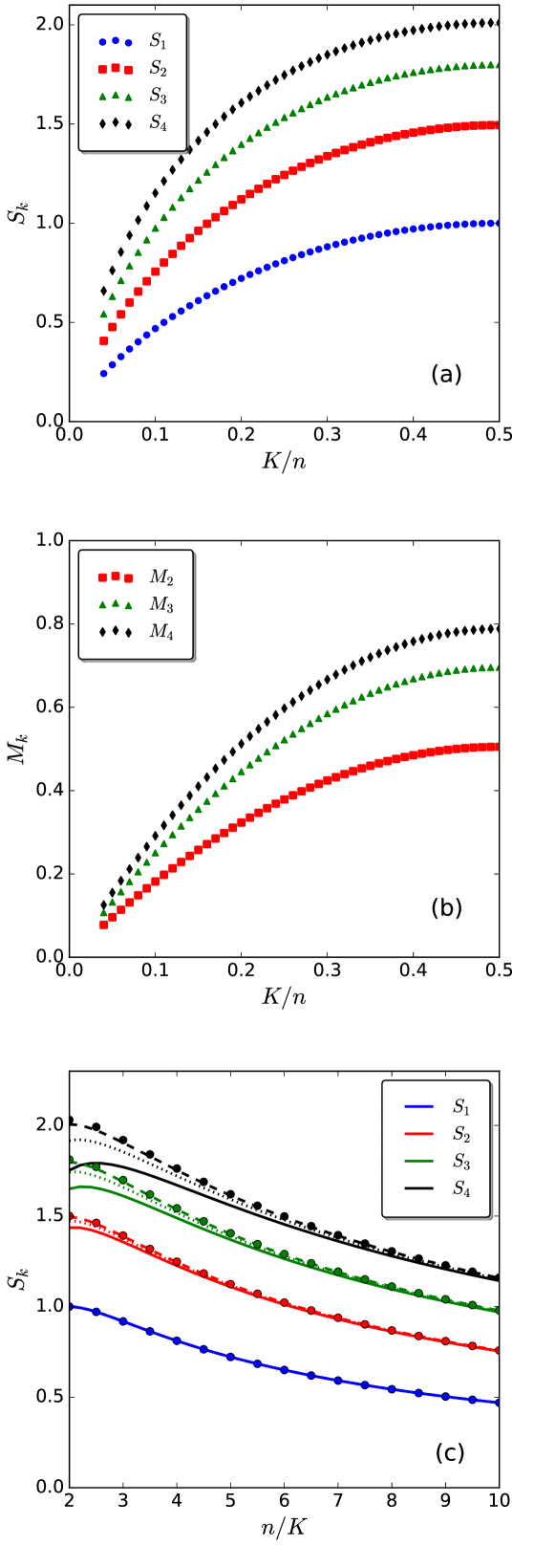
Figure 2: (a) $k$-qubit entropies for $k=1,\cdots,4$ of the state $|K,n\rangle$ obtained for the Dicke states for $n=100$ qubits with varying $4<K\leq n/2$ values. (b) Corresponding mutual information defined in Eq. (24) for $k=2,\cdots,4$. (c) Values of $S_{1,\cdots,4}$ for a state $|K,n\rangle$ with a fixed value of $K$ and increasing $n$ up to $n/K=10$. The solid line corresponds to $K=5$, dotted lines to $K=10$, while the dashed lines correspond to $K=40$. Note that all blue curves for $S_{1}$ are superimposed since, in this case, the one-qubit entropy is only a function of $K/n$. This figure also shows a set of curves displayed with filled circles corresponding to the binomial distribution with probability $P=K/n$.

III.1 Dicke/Total spin BTS

Dicke states correspond to the specific case where $x_{i}={\rm cte}$ in Eq. (2). For the sake of simplicity, I assume $x_{i}=1$ for all $i$ below. The entanglement entropies of these states have already been studied previously, for instance, in Ref. Mor18 . In particular, as further illustrated below, these states correspond to the maximally entangled states having the form given by Eq. (2). The Schmidt decomposition of the Dicke states was given in Ref. Mor18 using simple combinatoric developments. Alternatively, using the generating functions discussed above, we can immediately show that:

$$G^{m}_{l}({\cal S}) = C^{l}_{m},~{}~{}{\rm for}~{}l\leq m$$

and $G^{m}_{l}({\cal S})=0$ if $l>m$. This gives:

$$\lambda^{A}_{l} = \frac{C^{l}_{k}C^{K-l}_{n-k}}{C^{K}_{n}}.$$ (22)

We recognize here the hypergeometrical (HG) probability distribution, which is properly normalized to $1$ thanks to the Chu–Vandermonde identity wikiChuVandermond . A property that will be useful below is that the mean value and fluctuations of the Hamming weight, denoted generically as $\mu_{N}(A)$ and $\sigma^{2}_{N}(A)$ in the subsystem $A$. These two quantities are given by:

$$\mu_{N}(A)=k\frac{K}{n},~{}~{}\sigma^{2}_{N}(A)=k\left[\frac{n-k}{n-1}\right]\frac{K}{n}\left(1-\frac{K}{n}\right).$$ (23)

I illustrate here a few aspects of the Dicke state entanglement entropy. In Fig. 2-a are shown the entanglement entropy $S_{k}$ for a subsystem of size $k=1$ to $k=4$ and for various state $|K,n\rangle$. Note that only the cases $K/n\leq\nicefrac{{1}}{{2}}$ are shown because the curve is symmetric with respect to this point. This could indeed be understood from the fact that the number of $1$ and the number of $0$ plays a symmetric role with respect to the vertical line $K/n=\nicefrac{{1}}{{2}}$. Consequently, all $S_{k}$ with $k\leq K$ have a bell shape for $0\leq K/n\leq 1$ with a maximum exactly at $K/n=\nicefrac{{1}}{{2}}$. In order to illustrate the entanglement between particles, I also give in Fig. 2-b, the corresponding mutual information $M_{k}$ that I define for $k\geq 2$ as:

$$M_{k} = S_{k-1}+S_{1}-S_{k}.$$ (24)

This quantity gives a measure of the entanglement of one particle selected within the set of $k$ particles. We observe that the mutual information increases but this increase tends to be reduced as $k$ increases.

For small numbers of qubits $k$, I observed that the $S_{k}$ rapidly become independent from the absolute value of $K$ itself, but only depends on the ratio $K/n$ provided that $K\leq n/2$ is large enough and the number of sites $n$ itself is also large. A specific situation is the one-qubit entropy. In this case, we have directly:

$$S_{1} = -\frac{K}{n}\log_{2}\frac{K}{n}-\left(1-\frac{K}{n}\right)\log_{2}\left(1-\frac{K}{n}\right)$$ (25)

where we recognize the mean probability $P=K/n$ that the qubit is occupied. We see that $S_{1}$ is only dependent on the ratio $K/n$ and not on the specific value of $K$ or $n$ themselves. In Fig. 2-c, it is illustrated that this property is not true anymore for $S_{k}$ with $k>1$, but the $S_{k}$ are close to each other for the different $K$ values. This stems from the fact that:

$$\frac{C^{K-l}_{n-k}}{C^{K}_{n}} \longrightarrow \left(\frac{K}{N}\right)^{l}\left(1-\frac{K}{N}\right)^{k-l},$$ (26)

when both $K$ and $n$ are much larger than $l$ and $k$.

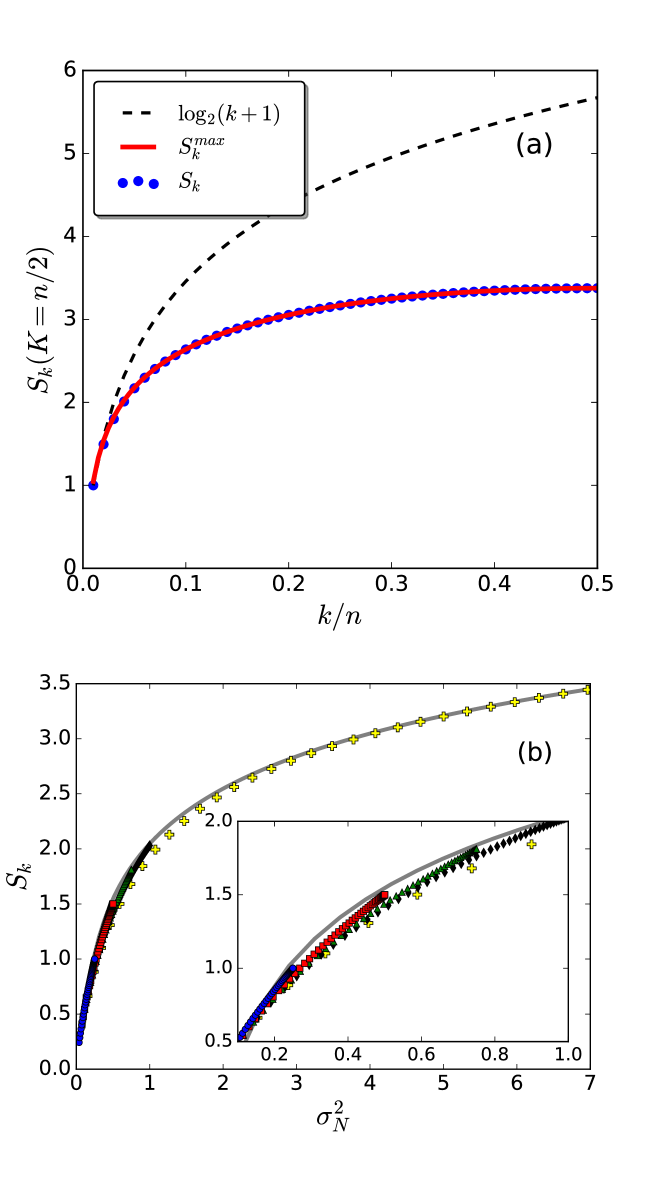
Figure 3: Panel a: Values of $S_{k}$ for the state $K=n/2$ with $n=100$ as a function of $k$. The black dashed line corresponds to the upper bound $\log_{2}(k+1)$. The red solid line corresponds to the $S^{\rm max}_{k}$ values given by Eq. (29). Panel b: $S_{k}$ for $k=1,\cdots,4$ (with the same symbols convention as in Fig. 2-a), for varying $K/n$ and $n=100$ as a function of the fluctuation of the Hamming weight $\sigma^{2}_{N}$ in the subspace $A$. The entropy is also shown for $k=K/2$ (yellow cross). The grey solid line corresponds to the Gaussian approximation, Eq. (27). The inset is a zoom on the small $\sigma^{2}_{N}$ values.

Accordingly, the corresponding coefficients $\lambda^{A}_{l}$ identify asymptotically with a binomial probability distribution that only depends on $P$. If we denote by $S^{\rm Bin}_{k}$ the entropy associated with a system of $k$ qubits where the equivalent binomial (bin) probability replaces the hypergeometric probability, we not only have $S^{\rm HG}_{k}\rightarrow S^{\rm bin}_{k}$, but also see in Fig. 2-c that $S^{\rm bin}_{k}$ is an upper bound for the $S_{k}$ entropy. This was checked numerically for all $(k,K)$ combinations up to $n=100$.

I conclude the discussion on the Dicke state entanglement properties by focusing on larger $k$ values in the system $A$. In Fig. 3-a is shown the evolution of $S_{k}$ with increasing $k$ for the specific state $|K=n/2,n\rangle$, and $n=100$. For small $k$ values, the entropy is rather close to the upper bound given by Eq. (19). As $k$ increases, we see a quenching of the entropy compared to this bound. To understand this quenching, the entropies for selected $k$ are displayed in Fig. 3-b as a function of the Hamming weight fluctuations given by Eq. (23) for varying $K/n$ ratio and $m=100$. We see in this figure that all entropies are very close to each other, showing that the fluctuations are driving the amplitude of the different entropies. We finally see in this figure that the curves are rather also close to the asymptotic limit

$$\tilde{S}_{k}=\frac{1}{2}\log_{2}(2\pi e\sigma^{2}_{N}),$$ (27)

that is expected when both $K$ and $n$ are large. Noteworthy, as shown in the inset, some deviations are observed for small $k$ values.

Despite these small deviations, one can use the expression of the fluctuations given by (23) to write an approximate form of the entropy as (for $k\leq K$):

$$\tilde{S}_{k} = \frac{1}{2}\log_{2}\left[2\pi eP(1-P)\right]+\frac{1}{2}\log_{2}k\left[\frac{n-k}{n-1}\right].$$ (28)

Several considerations can be made from this simple expression. The first term only depends on the ratio $K/n$, while the subsystem size dependence is contained in the second term. The first term is maximal for $P=1/2$. Although I do not give here a firm mathematical proof, the present study suggests an upper bound for the Dicke state entanglement, denoted by ${S}^{\rm max}_{k}$ obtained by setting $P=1/2$ in the previous expression, and given by:

$${S}^{\rm max}_{k} = \frac{1}{2}\log_{2}\left[\frac{\pi e}{2}\right]+\frac{1}{2}\log_{2}k\left[\frac{n-k}{n-1}\right].$$ (29)

The constant term gives approximately $c_{0}=\frac{1}{2}\log_{2}\left[\frac{\pi e}{2}\right]\simeq 1.047$. We see that we have respectively $S^{\rm max}_{1}=1.047$, $S^{\rm max}_{2}=1.55$, $S^{\rm max}_{3}=1.84$, and $S^{\rm max}_{4}=2.05$ that are just above the highest values of these entropies displayed in Fig. 2-c for $n/K=2$. We also see that ${S}^{\rm max}_{k}$ follows very closely the numerical values reported in Fig. 3-a, and properly accounts for the reduction compared to the limit given by (19). Note that, if we neglect the factor $(n-k)/(n-1)$ in Eq. (29), we get a slightly larger value ${S}^{\rm max}_{k}\sim\frac{1}{2}\log_{2}k+1$, that was obtained in Ref. Sto03 . However, the correction factor in Eq. (29) is important at large $k$ to reproduce the numerical values.

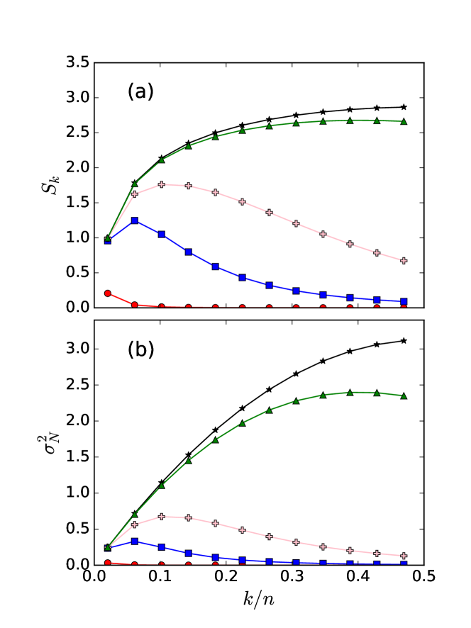
Figure 4: Illustration of the $k$-qubit/pairs entropy using BTS state inspired by the projected BCS theory (see text). (a) The entropy $S_{k}$ where $k$ is the number of ”qubits/pairs” within a certain energy window defined by an increasing $E_{\rm cut}$ is shown as a function of $k/n$. (b) fluctuations of particle number in the same energy window. The black solid line corresponds to the reference ”maximally entangled” Dicke state, e.g. with $|x_{i}|^{2}=1$ for all $i$. Different values of the parameter $\Delta/de$ are shown: $\Delta/de=1$ (red circles), $5$ (blue squares), $10$ (pink cross) and $50$ (green triangle). In all calculations, I used $n_{\rm st}=20$ ($n=49$) and assumed $K=n_{\rm st}$.

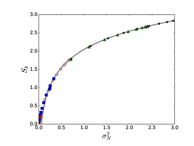
Figure 5: Same as in Fig. 4 except that now the entropy is shown as a function of the qubit/pair number fluctuations in the energy window. The conventions are the same as in Fig. 4 except that the lines connecting symbols are omitted for clarity. As in Fig. 3, the gray solid line corresponds to the Gaussian limit given by Eq. (27).

III.2 Projected BCS state

The projected BCS states are a second illustration of BTS states that motivated the present work. These states are used for small superfluid systems. Starting from their second quantized form given by Eq. (5), and using the pair encoding scheme Kha23 , BCS states can be expressed in terms of Pauli matrices as:

$$|\Phi(\{x_{i}\})\rangle = {\cal N}_{m}\prod_{i=1}^{m}\left(1+x_{i}\sigma^{+}_{i}\right)|0\rangle^{\otimes m}.$$ (30)

The $U(1)$ symmetry breaking associated with the fact that BCS states are not eigenstates of particle number transforms here into a mixing of states with different Hamming weights. Then, projected BCS is equivalent to projecting onto a specific Hamming weight equal to $K$, and after proper normalization, identify with the BTS state given by Eq. (2). It is interesting to mention that, although projected states will have non-trivial entanglement between pairs of particles, the BCS state given by (30), being written as simple unary operations on individual qubits, leads to zero mutual information between pairs.

To make contact with the standard physicist’s approach, I will consider below a set of states described by their single-particle energies $\{\varepsilon_{i}\}_{i=1,n}$ and assume that we have already solved BCS-like equations leading to a set of coefficients $(u_{i},v_{i})$. Having in mind the constant interaction pairing model, I parameterize these coefficients with two free parameters $(\lambda,\Delta)$:

$$|u_{i}|^{2}=\frac{1}{2}\left(1+\frac{\varepsilon_{i}-\lambda}{\sqrt{(\varepsilon_{i}-\lambda)^{2}+\Delta^{2}}}\right),$$

$$|v_{i}|^{2}=\frac{1}{2}\left(1-\frac{\varepsilon_{i}-\lambda}{\sqrt{(\varepsilon_{i}-\lambda)^{2}+\Delta^{2}}}\right).$$

The $x_{i}$ parameters in Eq. (30) can then be obtained from:

$$|x_{i}|^{2} = \frac{|v_{i}|^{2}}{|u_{i}|^{2}}=\frac{1-\frac{\varepsilon_{i}-\lambda}{\sqrt{(\varepsilon_{i}-\lambda)^{2}+\Delta^{2}}}}{1+\frac{\varepsilon_{i}-\lambda}{\sqrt{(\varepsilon_{i}-\lambda)^{2}+\Delta^{2}}}}.$$ (31)

Physically, $\lambda$ and $\Delta$ represent the Fermi energy and pairing gap, respectively. In the following, I assume that all $x_{i}$ are positive real numbers. Noteworthy, in the limit $\Delta\rightarrow+\infty$, all $|x_{i}|^{2}$ tend to $1$, and we recover the Dicke state limit.

As a numerical illustration, I consider below a set of $n=2n_{\rm st}+1$ equidistant levels with energies $\varepsilon_{i}$ distributed in $[-E_{\rm max},E_{\rm max}]$, and $\lambda=0$. I assume that $\Delta$ is a free parameter. Calculations below are made assuming $n=49$. We then have $E_{\rm max}=n_{\rm st}de$, where $de$ defines the level spacing. Single-particle energies are given by $\varepsilon_{i}=de(i-1-n_{\rm st})$ with $i=1,\cdots,n$. All energies will be given in $de$ units. I then assign to each site a $x_{i}$ coefficient given by Eq. (31) obtained by fixing the gap value $\Delta$. As before, the different qubits are separated into two subspaces $A$ and $\bar{A}$ and, for different splitting into two subspaces. I compute the reduced entropy of the subspace $A$ with varying numbers of sites included in $A$ and/or varying values of $\Delta$. In the illustration below, the subspace $A$ is built up as follows. $A$ corresponds to the subset of states respecting the condition $|\varepsilon_{i}|\leq E_{\rm cut}$, where $E_{\rm cut}$ is a cutoff energy, that we assume equal to $E_{\rm cut}/de=1/2+k_{c}$. The subspace size is then gradually increased by varying $k_{c}$ with $k_{c}=0,\cdots,n_{c}$ and $n_{c}=n_{\rm st}/2$ (here $n_{c}=10$). For a given $k_{c}$, the number of qubits/orbitals inside the energy window verifies $k=1+2k_{c}$.

In Fig. 4-a, the $k$-qubit entropy is displayed as a function of $k$, i.e., for increasing energy window size and for different values of $\Delta/de$. Panel b displays the fluctuations in the subspace $A$ of the pair number/Hamming weight of the projected BCS state. In Fig. 4, we see again that fluctuations in the subsystem $A$ and entropies are strongly correlated. As expected, as $\Delta$ increases, the entanglement entropy tends towards the Dicke state limits, corresponding to the upper limit of the projected BCS-type states. The strong correlations between entanglement and fluctuations are further evidenced in Fig. 5, where we recognize a similar behavior as we already observed in Fig. 3-b. We also see that, as soon as the fluctuations exceed a certain threshold, the correlations between $S_{k}$ and $\sigma^{2}_{N}$ closely follow the Gaussian asymptotic limits. Interestingly, this threshold that is around $\sqrt{\sigma^{2}_{N}}\simeq 0.5$ is rather low since it corresponds to a fluctuation of less than one particle unit. The validity of the Gaussian limit when considering part of a small superfluid, even for rather small systems, was already pointed out in Ref. Lac20 . Below this threshold in fluctuations, the Eq. (27) slightly underestimates the entropies uncovering the non-Gaussian nature of the fluctuations for very small subsystems.

IV Discussion on states decomposed on BTS states

In the present work, I concentrate on the specific entanglement entropy of a single BTS state $|K,n\rangle$. States like Dicke states provide a convenient basis when a system is described on a set of degenerated two-level systems labeled by $i=1,n$ and when the problem is invariant with respect to any permutation between indices of $(i_{1},\cdots,i_{n})$ labeling the 2-levels. An example of such a physical situation is the Lipkin model Lip65 ; Mes65 ; Gli65 . Here, I discuss a situation where the evolution of a permutation invariant system is considered. Its wave function can be decomposed at all times on the Dicke states as:

$$|\Psi(t)\rangle = \sum_{K}c_{K}(t)|K,n\rangle.$$ (32)

The block structure that has been made explicit above for each of the $|K,n\rangle$ state also exists for a state written as a linear combination of BTS states. To see this, I again split into two parts $(A,\bar{A})$ containing respectively $k$ and $(n-k)$ qubits/orbitals. I also rewrite Eq. (14) in a more compact form as:

$$|K,n\rangle = \sum_{l=0}^{K}g^{K}_{l}|l\rangle_{A}\otimes|K-l\rangle_{\bar{A}},$$

with $g^{K}_{l}=\sqrt{\lambda^{A}_{l}(K)}$, $|l,k\rangle_{A}\equiv|l\rangle_{A}$, and $|K-l,n-k\rangle_{\bar{A}}\equiv|K-l\rangle_{\bar{A}}$. Conditions given by Eq. (13) are accounted for simply by assuming that the $g^{K}_{l}=0$ if these conditions are not fulfilled. With this, we immediately see that the reduced density matrix of the subsystem $A$ is given by:

$$D_{A}(t) = \sum_{j,l=0}^{k}|j\rangle_{A}\left[{\cal D}^{A}_{jl}\right]{}_{A}\langle l|.$$ (33)

with the matrix elements

$${\cal D}^{A}_{jl}(t) = \sum_{K,L=0}^{n}c_{K}(t)c^{*}_{L}(t)g^{K}_{j}g^{J}_{l}\delta_{K-j,L-l}.$$ (34)

These matrix elements can be computed for any $k$ using the expression (19). This expression clearly underlines that only the coupling between permutation invariant states of the sub-system $A$ is relevant to discuss the entanglement entropy and that the subsystem entropy is also bound by Eq. (19), as expected from the symmetry of the problem. It also gives a practical way to calculate the entropy itself for any binary partition of the total system. Previous studies of the entanglement entropy for systems like the Lipkin model Fab22 ; Mom23 or neutrino Lac22 were mostly restricted to $k=1$ or $k=2$ and directly used the naive binary decomposition of the subsystem as schematically illustrated in Fig. 1. In Ref. Mom23 , the study of the 4-qubit entanglement entropy was made following the same strategy. This brute-force approach, which does not take advantage of the permutation symmetry rapidly becomes cumbersome and leads, for a given $k$, to the diagonalization of a matrix of size $2^{k}$. With the present method, the matrix $D_{A}(t)$ has a much lower dimension equal to $(k+1)$.

Contrary to the case of a single Dicke state where the entropy is bounded by Eq. (29), during the evolution of a system decomposed as in Eq. (32), larger entropies can be reached due to the additional mixing between Dicke states. In Ref. Lac22 , the absolute upper bound given by Eq. (19) was reached by coupling two different sets of two-level systems, called in this context neutrino beams, and allowing the simultaneous mixing of Dick states having both odd and even Hamming weight during the evolution.

V Summary and discussion

The binary tree structure of certain quantum ansätz allows us to derive compact forms of their entanglement entropies when the system is separated into two subsystems. The exact Schmidt decomposition of k-qubit can be obtained and eventually estimated at low numerical cost. With this, I study some quantum information properties of specific BTS states. The Dicke state’s scaling properties with fluctuations and upper bound of the entropies are analyzed. Since these states correspond to maximally entangled states having the BTS structure with fixed Hamming weight, the upper bound in entropy also holds for any BTS of such kind.

A second study is conducted on the entanglement properties of pairs in the projected BCS states. It is observed again that this entanglement is strongly correlated to the Hamming weight/pair number fluctuations and, in most situations very well described by the Gaussian entropy limit. This second class of states is standardly used in nuclear physics to describe in an effective way static and dynamical properties when the system wave-function is assumed to be a single quasi-particle vacuum. The properties derived here, therefore, should apply to this case, for instance, when cutting a system into two sub-parts.

I finally show that the technique developed here to numerically estimate the entanglement properties of BTS can also be useful to estimate similar entropies in systems whose wave functions decompose on a set of BTS states.

Acknowledgments. – The author is thankful to A. B. Balantekin, Amol V. Patwardhan, and Pooja Siwach for discussions at the early stage of the project especially on neutrino physics aspects. This project has received financial support from the CNRS through the AIQI-IN2P3 project. This work is part of HQI initiative (www.hqi.fr) and is supported by France 2030 under the French National Research Agency award number ”ANR-22-PNQC-0002”.

References

- (1) J.R. McClean, J. Romero, R. Babbush, A. Aspuru-Guzik, The theory of variational hybrid quantum-classical algorithms, New J. Phys. 18, 023023 (2016).
- (2) Y. Cao, J. Romero, J.P. Olson, M. Degroote, P.D. Johnson, M. Kieferová, I.D. Kivlichan, T. Menke, B. Peropadre, N.P.D. Sawaya, S. Sim, L. Veis, A. Aspuru-Guzik, Quantum chemistry in the age of quantum computing, Chem. Rev. 119, 10856 (2019).
- (3) S.McArdle, S.Endo, A.Aspuru-Guzik, S.C.Benjamin, X.Yuan, Quantum computational chemistry, Rev. Mod. Phys. 92, 015003 (2020).
- (4) B.Bauer, S.Bravyi, M.Motta, G.Kin-LicChan, Quantum algorithms for quantum chemistry and quantum Quantum Materials Science, Chem. Rev. 120, 12685 (2020).
- (5) K. Bharti, A. Cervera-Lierta, T.H. Kyaw, T. Haug, S. Alperin-Lea, A. Anand, M. Degroote, H. Heimonen, J.S. Kottmann, T. Menke, W.-K. Mok, S. Sim, L.-C. Kwek, A. Aspuru-Guzik, Noisy intermediate-scale quantum algorithms, Rev. Mod. Phys. 94, 015004 (2022).
- (6) S. Endo, Z. Cai, S.C. Benjamin, X. Yuan, Hybrid quantum-classical algorithms and quantum error mitigation, J. Phys. Soc. Jpn. 90, 032001 (2021).
- (7) T. Ayral, P. Besserve, D. Lacroix and A. Ruiz Guzman, Quantum computing with and for many-body physics, Eur. Phys. J. A 59 (2023).
- (8) Ignacio Cirac, David Perez-Garcia, Norbert Schuch, Frank Verstraete, Matrix Product States and Projected Entangled Pair States: Concepts, Symmetries, and Theorems, Rev. Mod. Phys. 93, 045003 (2021).
- (9) Caroline Robin, Martin J. Savage, and Nathalie Pillet, Entanglement rearrangement in self-consistent nuclear structure calculations, Phys. Rev. C 103, 034325 (2021).
- (10) Calvin W. Johnson, Oliver C. Gorton, Proton-neutron entanglement in the nuclear shell model , J. Phys. G: Nucl. Part. Phys. 50, 045110 (2023).
- (11) Aurel Bulgac, Entanglement entropy, single-particle occupation probabilities, and short-range correlations Phys. Rev. C 107, L061602 (2023).
- (12) Aurel Bulgac, Matthew Kafker, and Ibrahim Abdurrahman, Measures of complexity and entanglement in many-fermion systems, Phys. Rev. C 107, 044318 (2023) .
- (13) Ehoud Pazy, Entanglement entropy between short-range correlations and the Fermi sea in nuclear structure, Phys. Rev. C 107, 054308 (2023).
- (14) A. Pérez-Obiol, S. Masot-Llima, A. M. Romero, J. Menéndez, A. Rios, A. García-Sàez, B. Juliá-Díaz, Quantum entanglement patterns in the structure of atomic nuclei within the nuclear shell model, Eur. Phys. J. A 59, 240 (2023).
- (15) Javier Faba, Vicente Martín, and Luis Robledo, Correlation energy and quantum correlations in a solvable model, Phys. Rev. A 104, 032428 (2021).
- (16) Javier Faba, Vicente Martín, and Luis Robledo, Analysis of quantum correlations within the ground state of a three-level Lipkin model, Phys. Rev. A 105, 062449 (2022).
- (17) Sébastien Dusuel and Julien Vidal, Finite-Size Scaling Exponents of the Lipkin-Meshkov-Glick Model, Phys. Rev. Lett. 93, 237204 (2004).
- (18) Julien Vidal, Rémy Mosseri, and Jorge Dukelsky, Entanglement in a first-order quantum phase transition, Phys. Rev. A 69, 054101 (2004)
- (19) Julien Vidal, Guillaume Palacios, and Rémy Mosseri, Entanglement in a second-order quantum phase transition, Phys. Rev. A 69, 022107 (2004).
- (20) Julien Vidal, Guillaume Palacios, and Claude Aslangul, Entanglement dynamics in the Lipkin-Meshkov-Glick model, Phys. Rev. A 70, 062304 (2004).
- (21) M. Di Tullio, R. Rossignoli, M. Cerezo, and N. Gigena, Fermionic entanglement in the Lipkin model, Phys. Rev. A 100, 062104 (2019)
- (22) Chenyi Gu, Z. H. Sun, G. Hagen, T. Papenbrock, Entanglement entropy of nuclear systems, Phys. Rev. C 108, 054309 (2023).
- (23) Christopher J. Stein and Markus Reiher, Automated Selection of Active Orbital Spaces, J. Chem. Theory Comput. 12, 1760 (2016).
- (24) Christopher J. Stein and Markus Reiher, Autocas: A program for fully automated multiconfigurational calculations, J. Comput. Chem. 40, 2216 (2019).
- (25) S. Momme Hengstenberg, Caroline E. P. Robin, Martin J. Savage, Multi-Body Entanglement and Information Rearrangement in Nuclear Many-Body Systems, Eur. Phys. J. A 59, 231 (2023).
- (26) A. Tichai, S. Knecht, A.T. Kruppa, O. Legeza, C.P. Moca, A. Schwenk, M.A. Werner, G. Zarand, Combining the in-medium similarity renormalization group with the density matrix renormalization group: Shell structure and information entropy, Phys. Lett. B 845, 138139 (2023).
- (27) B. Li, D. Vretenar, T. Niksic, D. D. Zhang, P. W. Zhao, J. Meng, Entanglement in multinucleon transfer reactions, arxiv:2403.19288.
- (28) M. A. Nielsen and I. L. Chuang. Quantum information and quantum computation., Cambridge University Press (2000).
- (29) Luigi Amico, Rosario Fazio, Andreas Osterloh, and Vlatko Vedral, Entanglement in many-body systems, Rev. Mod. Phys. 80, 517 (2008).
- (30) R. Horodecki, P. Horodecki, M. Horodecki, and K. Horodecki, Quantum entanglement, Rev. Mod. Phys. 81, 865 (2009).
- (31) N. Laflorencie, Quantum entanglement in condensed matter systems, Phys. Rep. 646, 1 (2016)
- (32) Anubhav Kumar Srivastava, Guillem Müller-Rigat, Maciej Lewenstein and Grzegorz Rajchel-Mieldzioć, Introduction to quantum entanglement in many-body systems, arxiv:2402.09523
- (33) Denis Lacroix, A. B. Balantekin, Michael J. Cervia, Amol V. Patwardhan, and Pooja Siwach, Role of non-Gaussian quantum fluctuations in neutrino entanglement, Phys. Rev. D 106, 123006 (2022).
- (34) Armin Khamoshi, Rishab Dutta, and Gustavo E. Scuseria, State Preparation of Antisymmetrized Geminal Power on a Quantum Computer without Number Projection, The Journal of Physical Chemistry A 127, 4005 (2023).
- (35) Rishab Dutta, Fei Gao, Armin Khamoshi, Thomas M. Henderson, Gustavo E. Scuseria, Correlated pair ansatz with a binary tree structure, arXiv:2310.20076
- (36) R. H. Dicke, Coherence in spontaneous radiation processes, Phys. Rev. 93, 99 (1954).
- (37) A. Messiah, Quantum mechanics, vol. II. (North-Holland, Amsterdam, 1962).
- (38) Per‐Olov Löwdin and Osvaldo Goscinski The exchange phenomenon, the symmetric group, and the spin degeneracy problem, International Journal of Quantum Chemistry vol. 4, S3B, 533 (1969).
- (39) P. Ring and P. Schuck, The Nuclear Many-Body Problem (Springer-Verlag, New-York, 1980).
- (40) J. P. Blaizot and G. Ripka, Quantum Theory of Finite Systems, (MIT Press, Cambridge, 1986).
- (41) Jan von Delft, D.C. Ralph, Spectroscopy of discrete energy levels in ultrasmall metallic grains, Phys. Rep. 345, 61 (2001).
- (42) D.M. Brink and R.A. Broglia, Nuclear Superfluidity: Pairing in Finite Systems, Cambridge University Press (2005).
- (43) P. Jordan and E. Wigner, Über das Paulische Äquivalenzverbot, Z. Phys. 47, 631 (1928).
- (44) Elliott Lieb, Theodore Schultz, Daniel Mattis, Two soluble models of an antiferromagnetic chain, Ann. of Phys. 16, 407 (1961).
- (45) A. Khamoshi, T. Henderson, and G. Scuseria, Correlating AGP on a quantum computer, Quant. Sci. Technol. 6, 014004 (2021).
- (46) E. A. Ruiz Guzman and D. Lacroix, Accessing ground-state and excited-state energies in a many-body system after symmetry restoration using quantum computers, Phys. Rev. C 105, 024324 (2022). doi:10.1103/PhysRevC.105.024324.
- (47) E. A. Ruiz Guzman and D. Lacroix, Restoring broken symmetries using quantum search “oracles”, Phys. Rev. C 107 (2023) 034310.
- (48) D. Lacroix, E. A. Ruiz Guzman, and P. Siwach, Symmetry breaking/symmetry preserving circuits and symmetry restoration on quantum computers Eur. Phys. J. A 59, 3 (2023).
- (49) E. A. Ruiz Guzman and D. Lacroix, Restoring symmetries in quantum computing using Classical Shadows , arXiv:2311.04571
- (50) N. Sandulescu and G. F. Bertsch, Accuracy of BCS-based approximations for pairing in small Fermi systems Phys. Rev. C 78, 064318 (2008).
- (51) N. Sandulescu, B. Errea, and J. Dukelsky, Isovector neutron-proton pairing with particle number projected BCS, Phys. Rev. C 80, 044335 (2009).
- (52) Denis Lacroix and Guillaume Hupin, Density-matrix functionals for pairing in mesoscopic superconductors, Phys. Rev.B 82, 144509 (2010).
- (53) Guillaume Hupin and Denis Lacroix, Description of pairing correlation in many-body finite systems with density functional theory, Phys. Rev. C 83, 024317 (2011).
- (54) D. Lacroix, Symmetry-Assisted Preparation of Entangled Many-Body States on a Quantum Computer, Phys. Rev. Lett. 125 (2020) 230502. doi:10.1103/PhysRevLett.125.230502.
- (55) P. Siwach and D. Lacroix, Filtering states with total spin on a quantum computer , Phys. Rev. A 104, 062435 (2021).
- (56) Claude Cohen-Tannoudji, Bernard Diu, and Franck Laloë. Quantum Mechanics Volume 2. (Hermann, 1986).
- (57) M. G. M. Moreno, Fernando Parisio, All bipartitions of arbitrary Dicke states, arXiv:1801.00762
- (58) John K. Stockton, J. M. Geremia, Andrew C. Doherty, and Hideo Mabuchi, Characterizing the entanglement of symmetric many-particle spin-1/2 systems Phys. Rev. A 67, 022112 (2003).
- (59) V. N. Fomenko, Projection in the occupation-number space and the canonical transformation, J. Phys. A: Gen. Phys. 3, 8 (1970).
- (60) https://en.wikipedia.org/wiki/Vandermonde%27s_identity
- (61) Denis Lacroix and Sakir Ayik, Counting statistics in finite Fermi systems: Illustrations with the atomic nucleus, Phys. Rev. C 101, 014310 (2020).
- (62) H. J. Lipkin, N. Meshkov and A. J. Glick, Validity of many-body approximation methods for a solvable model: (I) Exact solutions and perturbation theory, Nucl. Phys. A 62, 188 (1965).
- (63) N. Meshkov, A. Glick, and H. Lipkin, Validity of many-body approximation methods for a solvable model: (II). Linearization procedures, Nucl. Phys. 62, 199 (1965).
- (64) A. Glick, H. Lipkin, and N. Meshkov, Validity of many-body approximation methods for a solvable model: (III). Diagram summations, Nucl. Phys. 62, 211 (1965).