Classification of Breast Cancer Histopathology Images using a Modified Supervised Contrastive Learning Method

Abstract

Deep neural networks have reached remarkable achievements in medical image processing tasks, specifically classifying and detecting various diseases. However, when confronted with limited data, these networks face a critical vulnerability, often succumbing to overfitting by excessively memorizing the limited information available. This work addresses the challenge mentioned above by improving the supervised contrastive learning method to reduce the impact of false positives. Unlike most existing methods that rely predominantly on fully supervised learning, our approach leverages the advantages of self-supervised learning in conjunction with employing the available labeled data. We evaluate our method on the BreakHis dataset, which consists of breast cancer histopathology images, and demonstrate an increase in classification accuracy by 1.45% at the image level and 1.42% at the patient level compared to the state-of-the-art method. This improvement corresponds to 93.63% absolute accuracy, highlighting our approach’s effectiveness in leveraging data properties to learn more appropriate representation space. The code implementation of this study is accessible on GitHub.

1 Introduction

Cancer, a leading cause of mortality worldwide, poses a significant threat to public health. Among the various types of cancer, breast cancer is the most prevalent form affecting women, resulting from abnormal cell division in the breast tissue. However, it is essential to note that not all tumors are life-threatening, as they can be either benign or malignant, and detecting a tumor’s malignancy or benign nature is crucial in determining appropriate treatment strategies and ensuring patient well-being.

Medical imaging stands out as one of the most commonly used artificial intelligence applications in healthcare. The research focused on applying machine learning to medical images, which demonstrates significant potential in revolutionizing the diagnostic process of various cancerous diseases by enabling the early detection and accurate characterization of tumors. However, several challenges within the medical field are delaying the widespread utilization of machine-learning capabilities in real-world applications. These challenges include the generalization issues of Deep Neural Networks, collecting diverse data sets, acquiring sufficient labeled data for training, and the risks and high costs associated with errors in medical decision-making. The growing importance of these methods in the medical domain highlights the urgent need to implement effective approaches to overcome these challenges more than ever.

The classification of medical images plays a supportive role in clinical treatment. Histopathology also greatly benefits from the application of machine learning techniques. Leveraging the power of machine learning in diagnosing cancerous images has the potential to revolutionize the field, aiding pathologists in making precise diagnoses and facilitating the treatment process. However, due to the critical nature of this issue and the potential risks, the widespread use of these methods is still limited. As a result, it is crucial to focus on reducing existing errors by examining earlier methods and striving to improve upon them. Supervised methods previously used for image classification have limitations, as they require a considerable amount of labeled data, and collecting them usually requires a high cost. Fortunately, in recent years, self-supervised learning has emerged as a promising approach, presenting its effectiveness in various tasks.

The contributions of this work are focused on overcoming the challenges associated with training networks in the context of cancer image diagnosis. One of the main challenges this study addresses is the scarcity of labeled data in the medical domain, which poses difficulties for supervised learning approaches. To tackle this issue, the proposed method draws inspiration from self-supervised learning techniques and extends them by utilizing labeled data and leveraging similarities between images in the representation space. Additionally, to address the problem of generalization in deep neural networks, various data augmentation techniques specific to histopathology datasets and H&E stains are employed to enhance the robustness and generalization capabilities of the trained models.

The primary objective of this study is to develop a method that improves the accuracy of cancer image diagnosis in two publicly available breast cancer datasets. The proposed method considers all available magnifications, ensuring comprehensive and accurate classification of the images. The method’s effectiveness is evaluated by comparing it to previous works, and a detailed analysis of the obtained results is presented at the end.

2 Literature Review

Over the past few years, machine learning has achieved remarkable progress in developing systems by leveraging large amounts of labeled data. While this learning approach has shown excellent performance in previous tasks, it faces limitations in medical applications due to the issue of data scarcity.

Self-supervised learning is an approach that does not need labeled data to train the deep models. It can be divided into two main subcategories: contrastive and non-contrastive. Contrastive learning aims to maximize the similarity between positive pairs and minimize the similarity between negative pairs, e.g., SimCLR [3], SimCLRv2 [4], and PIRL [18] are based on this approach. On the other hand, non-contrastive learning methods work in other ways; for example, they focus only on maximizing the similarity between positive pairs since finding negative pairs can be challenging when working with unlabeled data. Some examples of non-contrastive learning e.g. BYOL [10], DirectPred [25], and SimSiam [5]. Furthermore, a more effective approach to contrastive learning is to utilize the labels associated with the data to guide the choice of negative and positive pairs, where positive pairs consist of samples that belong to the same class, and negative pairs are formed by taking samples from different classes [15].

Research results on medical images using self-supervised methods demonstrate better performance than the supervised ones. For instance, Chhipa et al. [6] introduced a method based on the Efficient-net [23] architecture that utilizes the SimCLR approach for the binary classification of the BreakHis dataset. Jin et al. [14] introduced the HistoSSL architecture, a knowledge distillation model based on non-contrastive learning, which does not rely on a strategy for creating negative pairs. Additionally, Li et al. [16] proposed a combined method of SimCLR and multiple instance learning [8], in which the representations of an image are extracted through self-supervised learning and given as input to a multiple instance learning model. Ciga et al. [7] presented a relatively comprehensive article using the self-supervised SimCLR method on different ResNet [11] architectures, i.e. ResNet-18, ResNet-34, ResNet-50, and ResNet-101. The network was trained in a self-supervised manner on 57 different histopathology datasets, and ultimately, the weights obtained were used for classification, segmentation, and regression tasks on the data.

The cases mentioned above represent only a few examples of the research conducted in the field of histopathology for self-supervised learning. There is comparatively less research in this area than in supervised learning, creating an opportunity for progress and advancement, as demonstrated in this report.

3 Method

This work mainly focuses on leveraging the advantages of self-supervised learning to extract high-quality representations from images. However, as self-supervised learning may produce false negatives and positives when creating the pairs, we complement it with supervised learning, which uses image labels, to mitigate these effects.

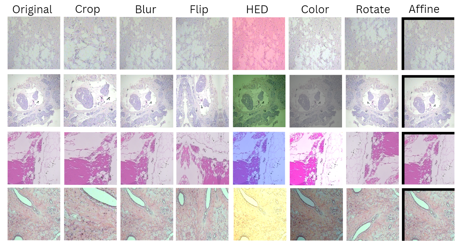
Figure 1: Data augmentation strategies. In this figure, an illustration of the various data augmentation methods used in the research is provided.

First, the model is trained on five distinct breast cancer datasets, with the SimCLR technique to establish a solid starting point. We then utilize these pre-trained weights as the initial weights for our representation learning phase. The representation learning phase includes a two-stage supervised contrastive learning. Following this, supervised fine-tuning is accomplished wherein three fully connected layers are added to the end of the encoder for classification task and one fully connected layer is employed for an auxiliary task. Ultimately, four identical architectures are employed in the dataset and trained separately for four magnification factors.

3.1 Augmentations

The initial step in using a self-supervised approach is to generate positive and negative pairs. In this study, two techniques were employed to create such pairs.

The most prevalent way of creating positive pairs is through augmentation. In this study, various methods were utilized for this purpose, including Random Crop, Color Jitter, Gaussian Blur, and Geometric, which are depicted in Figure 1. All of the mentioned augmentations are applied with a fixed probability to create the image pairs, and the resulting pairs can be observed in Figure 2.

Furthermore, a histopathology-specific augmentation technique known as HED [24] has been employed. This method involves separating the two H&E stains from the RGB images, adjusting the brightness and contrast of each stain’s corresponding matrix individually, and then converting them from the H&E channel to the RGB. This process serves as a data augmentation method for creating positive pairs and also enhances the model’s ability to generalize against different stains. These stains can be separated using the following formula [27].

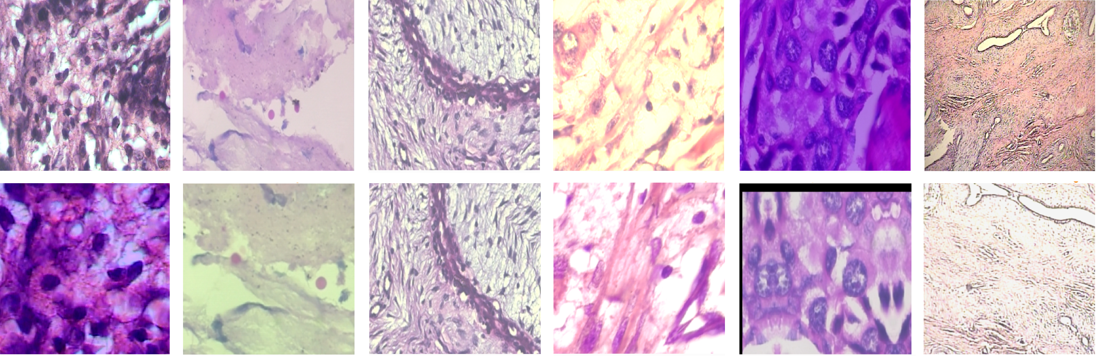
Figure 2: Positive pairs. This figure depicts an anchor image alongside one of its corresponding positive pairs. This pair is created through a combination of data augmentations introduced in figure 1, and each augmentation is applied with a specific probability. The first row indicates the anchor image, while the second one is donated to the corresponding positive pair.

$$V=log\frac{I_{0}}{I}=WH$$ (1)

According to Beer-lambert law $I\in R^{3\times n}$ is the RGB density matrix, and $I_{0}$ is equal to 255. $V\in R^{3\times n}$ is an optical density matrix, $W\in R^{3\times 2}$ is the conversion matrix, and $H\in R^{2\times n}$ is the stain matrix[26]. The following optimization problem is utilized to find desired factorization:

$$\begin{split}\min_{W,H}\frac{1}{2}||V-WH||^{2}_{F}+\lambda\sum^{2}_{j=1}||H(j,:)||_{1},\\ s.t\>W,H\geq 0,||W(:,j)||^{2}_{2}=1\end{split}$$ (2)

By solving this sparse non-negative matrix factorization problem mentioned above, $W$ and $H$ can be estimated [27]. $H$ is the converted matrix, from RGB image to $H$ and $E$ arrays. Subsequently, in HED augmentation, the contrast and brightness of $I_{h}$ and $I_{e}$ are altered as:

$$I_{h}=aug(I_{0}exp(-H[0,:])),I_{e}=aug(I_{0}exp(-H[1,:]))$$ (3)

Finally, stains are converted back into the RGB color space using the $W$ matrix [27].

3.2 Contrastive Representation Learning

In this phase, we have two stages of training with the contrastive method, as illustrated in Figure 3.

3.2.1 Modified Supervised Contrastive Learning

First, we extract the representation using a modified supervised contrastive loss, which takes the following form.

$$\ell_{i}=\frac{-\alpha}{|P(i)|}\sum_{p\in P(i)}\log(\frac{exp(z_{i}\cdot z_{p}/\tau)}{\sum_{p\in P(i)}exp(z_{i}\cdot z_{p}/\tau)+\lambda\sum_{q\in Q(i)}exp(z_{i}\cdot z_{q}/\tau)})$$ (4)

During the first stage, positive pairs are created using augmentations and image labels. In this context, $i$ is the index of the anchor image. Assuming a set $A$ comprising $2N-1$ samples from both images and their corresponding augmented pairs, derived from a batch of size $N$, we define $P$ as the subset of images within set $A$ sharing the same label as the anchor and $Q$ as the subset containing images with different labels from the anchor. The representation of the anchor image is denoted as $z_{i}$, while $z_{p}$ represents one of the positive pairs for $z_{i}$ in the $P$ set. Similarly, $z_{q}$ denotes a negative pair for $z_{i}$ in the $Q$ set. Furthermore, $\alpha$ is the weight assigned to this loss function, which is calculated with respect to the number of samples in both classes to overcome the class imbalance issue. The utilization of the dot product instead of similarity stems from the fact that the data is normalized.

Eq. 4, presented in this method, is derived from a combination of three loss functions: self-supervised loss [3], supervised contrastive loss [15], and elimination loss [12]. The specific formulas for each of these loss functions are described below:

$$\ell_{self(i)}=-log(\frac{exp(z_{i}\cdot z_{j}/\tau)}{\sum_{k=1}^{2N}\mathbbm{1}_{k\neq i}exp(z_{i}\cdot z_{k}/\tau)})$$ (5)

$$\ell_{sup(i)}=\frac{-1}{|P(i)|}\sum_{p\in P(i)}log(\frac{exp(z_{i}\cdot z_{p}/\tau)}{\sum_{k=1}^{2N}\mathbbm{1}_{k\neq i}exp(z_{i}\cdot z_{a}/\tau))})$$ (6)

$$\ell_{elim(i)}=-log(\frac{exp(z_{i}\cdot z_{j}/\tau)}{\sum_{k=1}^{2N}\mathbbm{1}_{[k\neq i,k\notin P(i)]}exp(z_{i}\cdot z_{k}/\tau)}).$$ (7)

The structure of our presented loss function is similar to Eq. 6. By introducing a coefficient $\lambda$ and the $Q$ set, we have incorporated the effect of the Eq. 7. Additionally, by utilizing augmentations for creating a positive pair for images, we have also integrated the impact of Eq. 5 into our approach. These losses and their individual effectiveness are further analyzed in the result section.

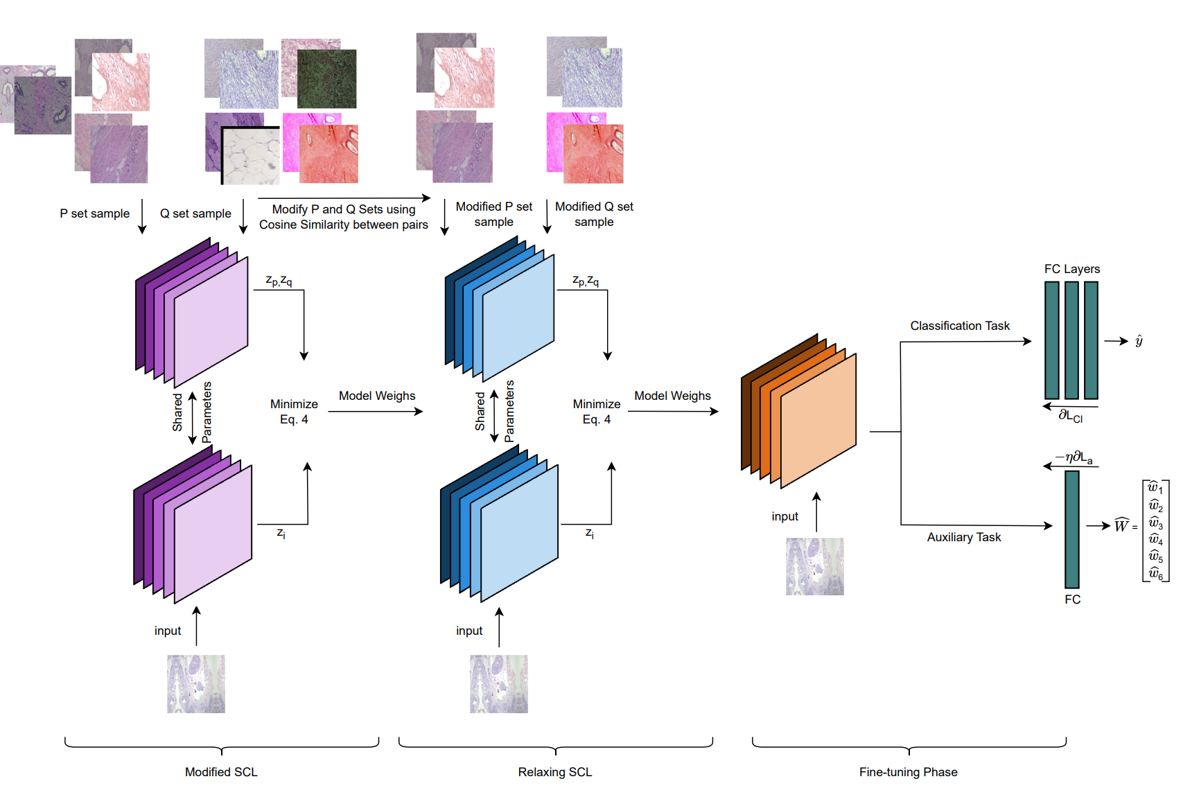
Figure 3: Network architecture. The architecture consists of three training stages, starting with the weights of EfficientNet pre-trained on histopathology images. The pre-training phase involves training on the Breakhis dataset using the modified supervised contrastive learning method. Subsequently, the similarity between the image representations is calculated to correct the positive pairs, followed by retraining with the updated set of pairs in the relaxing phase. The final stage is fine-tuning, which involves an auxiliary and classification task using a supervised approach. Here, the representation of the anchor image is denoted as $z_{i}$, while $z_{p}$ and $z_{q}$ are the representation of a positive pair and a negative pair, respectively. $\hat{y}$ and $\hat{W}=(\hat{w_{1}},\hat{w_{2}},\hat{w_{3}},\hat{w_{4}},\hat{w_{5}},\hat{w_{6}})$ are the predicted label, and conversion matrix with respect to the input image.

3.2.2 Relaxing Supervised Contrastive Learning

Once the model has been trained using this loss function, its weights are loaded to calculate the cosine similarity between all pairs of images in the dataset.

In the relaxing stage, the positive pairs are created like in the previous phase. However, the set $P$ is altered in such a way that if an image in the $P$ set has a similarity score less than 0.5 in the obtained representation space, it is removed from the $P$ set and is no longer considered a positive pair. This means that if, after the model is trained, assuming the $i$-th image is a positive pair for the anchor, which shows negative similarity in the resulted representation space, then it is not a good positive pair. More precisely, it does not have enough similarity even after enforcing it to be similar to the anchor, and so it is removed from the $P$ set. The same technique goes for the $Q$ set: if an image in the $Q$ set has a similarity score of more than 0.5 in the obtained representation space, it is removed from the $Q$ set and is no longer considered a negative pair.

In this stage, we continue to use the same loss function as Eq. 4. However, in contrast to the first stage, $z_{p}$ now represents a positive pair in the $P$ set and is greater than $0.5$ in similarity with the anchor. Similarly, $z_{q}$ denotes a negative pair for $z_{i}$ in the $Q$ set and less than $0.5$ similarity with the anchor. The proposed contrastive learning method is summarized briefly in Algorithm 1.

3.3 Fine-tuning

In this stage, the weights generated during the relaxing phase are fine-tuned via a supervised process using the labeled data. This supervised process comprises a primary classification task and an auxiliary task.

3.3.1 Classifier

This architecture, depicted in Figure 3, is designed to perform binary image classification. To accomplish this task, a classification head consisting of three fully connected layers is added at the end of the encoder. This loss function is computed using the following equation.

$$L_{Cl}=\frac{1}{N}\sum_{i=1}^{N}\mathcal{L}_{CE}(\hat{y_{i}},y_{i})$$ (8)

$y_{i}$ is the ground truth label for $x_{i}$, and $\hat{y_{i}}$ is the network’s output for the classification task. $\mathcal{L}_{CE}$ is the Cross-Entropy classification loss.

3.3.2 Auxiliary Task

An auxiliary task is also incorporated to improve the network’s robustness against different H&E stains by adding one fully connected layer at the end of the encoder [17].

Algorithm 1 Improved Supervised Contrastive Learning

Input: Efficient-net2 model, training dataset $X_{train}$

Output: Efficient-net2 weighs $W$

1:Initialize $P$, and $Q$ sets for each image, $x_{i}$, using data augmentations and the labels

2:calculate Eq. 4, which Maximize similarity between $x_{i}$ and its $P$ set in a batch while minimize similarity between $x_{i}$ and the batch images with double focus ($\lambda=2$) on ones from the $Q$ set in the representation space

3:Train for 200 epochs

4:Calculate similarity between the representation of all image pairs

5:If similarity $<0.5$ remove from $P$ set

6:If similarity $>0.5$ remove from $Q$ set

7:Repeat step 2, and 3.

8:Return $W$

The output of this task is a six-element matrix, which predicts the W matrix in Eq. 1. The loss function associated with this branch calculates the difference between the predicted and original matrices. This loss function is computed using the following equation.

$$L_{a}=\frac{1}{N}\sum_{i=1}^{N}\mathcal{L}_{a}(\hat{W_{i}},W_{i})$$ (9)

where $W_{i}$ is the matrix that transforms the input image from the RGB space to the H&E space, and $\hat{W_{i}}$ is the network’s output for the auxiliary task. $\mathcal{L}_{a}$ measures the difference between the predicted and original transformation matrices using Squared L2.

The resulting loss value is then fed back to the network with a negative sign to reduce the model’s sensitivity to variations in stain colors. The experiments showed that incorporating the auxiliary task alone does not significantly improve the model’s accuracy. However, to leverage the benefits of this technique, images must first be augmented using HED and then provided as inputs to the encoder. Moreover, during the fine-tuning stage, other data augmentation methods are utilized to further enhance the model’s generalization capabilities and increase the learning process’s robustness.

3.3.3 Final Loss

The final loss function is calculated by combining the classification loss and auxiliary loss with the coefficient $\eta$. The equation is as follows:

$$Loss=L_{Cl}-\eta L_{a}$$ (10)

4 Experiment and Results

This section investigates the experimental evaluation of the proposed method on two publicly available datasets and compares its results with those of previous methods.

4.1 Datasets

1. BreakHis [22]. This dataset consists of 7,909 stained microscopic images of breast tumor tissue collected from 82 patients. The images are captured at four different magnification factors, namely, $40X$, $100X$, $200X$, and $400X$. The dataset consists of two primary breast tumor categories, classified as benign or malignant. Specifically, there are 2,480 samples from benign patients and 5,429 from malignant patients. The BreakHis dataset is imbalanced, with significantly more samples in the malignant class. To mitigate the impact of this issue, a weighted loss function was used during all three training stages.

2. BACH [1]. This dataset comprises 400 stained microscopic images and 30 whole slide images of breast tumor tissue. The microscopic images have been categorized into normal and benign techniques that have been employed in previous studies, such as those cited in [28]in situ carcinoma and invasive carcinoma, with each category containing 100 images. The purpose of employing the BACH dataset was to evaluate the generalization of our backbone, which was trained using the BreakHis dataset. As the research objective revolves around the binary classification of breast tumors, a few adjustments were made to the labels in the BACH dataset. The normal and benign labels were treated as benign, while the in situ carcinoma and invasive carcinoma labels were considered malignant. Previous studies have employed similar techniques, such as those cited in [28] and [19].

To conduct the experiments, the datasets were split into training, test, and validation sets in a $60\%,20\%,20\%$ ratio, respectively, and the experiments were repeated for 5 folds to ensure accurate results.

4.2 Experimentation Details

The EfficientNet-B2 [23] is an encoding architecture that is utilized in this study. To ensure a solid starting point, we begin by randomly assigning the Efficient-Net2 weights. Subsequently, we train the model using SimCLR on five distinct breast cancer datasets: andrewjanowczyk epi [13], andrewjanowczyk mitosis [13], andrewjanowczyk nuclei [13], Mitos & Atypia [20], and IDCGrad [2]. In order to evaluate the performance of the proposed model for binary classification of the BreakHis dataset, five previous networks were chosen as benchmarks. Then, their performance was assessed by comparing the Image-Level Accuracy (the average accuracy across all images) and the Patient-Level Accuracy (the average accuracy for individual patients) against the performance of the proposed model.

The network is trained for $200$ epochs in the first two stages. During this process, the temperature of $0.01$, the learning rate $10^{-5}$, and a set of augmentations is utilized. The Adam optimizer is also employed as the optimization function, the batch size is set to $12$, and the $\lambda$ parameter is equal to $2$.

In the next stage of training, i.e., the supervised fine-tuning phase, the four distinct models, each for one magnification factor, are trained for only $20$ epochs. The learning rate is set to $2\times 10^{-5}$, and augmentations are applied to enhance the network’s generalization capabilities. Furthermore, the number of fully connected layers and neurons in each layer are determined through hyperparameter tuning. Additionally, dropout with a probability of $0.5$ is implemented between the fully connected layers, the batch size is 8, and the $\eta$ parameter for the auxiliary task is set to $0.5$.

Table 1: Comparison of image-level accuracy with previous methods for four magnification factors of the BreakHis dataset.

Methods	40X	100X	200X	400X	Mean
pdMISVM	$87.92\pm 0.9$	$89.04\pm 2.4$	$88.91\pm 2.1$	$85.78\pm 1.9$	$87.91\pm 1.8$
DenseNet121	$\bm{94.26\pm 3.2}$	$92.71\pm 0.4$	$83.90\pm 2.8$	$82.74\pm 1.5$	$88.40\pm 2.0$
ResHist-Aug	$87.40\pm 3.0$	$87.26\pm 3.5$	$91.15\pm 2.3$	$86.27\pm 2.2$	$88.02\pm 2.8$
MPCS-OP	$93.26\pm 3.4$	$93.45\pm 2.9$	$92.45\pm 3.8$	$89.57\pm 3.0$	$92.18\pm 3.3$
MPCS-RP	$92.72\pm 3.9$	$92.72\pm 4.0$	$91.91\pm 3.2$	$88.56\pm 3.9$	$91.48\pm 3.7$
Ours	$93.00\pm 2.8$	$\bm{93.51\pm 2.1}$	$\bm{95.28\pm 1.9}$	$\bm{92.73\pm 1.8}$	$\bm{93.63\pm 2.2}$

Table 2: Comparison of patient-level accuracy with previous methods for four magnification factors of the BreakHis dataset.

Methods	40X	100X	200X	400X	Mean
PFTAS	$82.03\pm 2.8$	$81.02\pm 3.9$	$83.58\pm 3.1$	$81.17\pm 4.4$	$81.95\pm 3.6$
DenseNet121	$92.02\pm 0.9$	$90.21\pm 2.4$	$81.94\pm 1.7$	$80.09\pm 0.7$	$86.06\pm 1.4$
ResHist-Aug	$87.47\pm 3.2$	$88.15\pm 3.0$	$92.52\pm 2.8$	$87.78\pm 2.5$	$88.98\pm 2.9$
MPCS-OP	$93.00\pm 3.7$	$93.26\pm 3.1$	$92.28\pm 2.9$	$88.74\pm 3.9$	$91.82\pm 3.3$
MPCS-RP	$92.72\pm 3.5$	$\bm{93.57\pm 2.9}$	$92.23\pm 3.9$	$88.40\pm 3.1$	$91.73\pm 3.3$
Ours	$\bm{93.99\pm 3.0}$	$91.34\pm 6.6$	$\bm{94.80\pm 2.4}$	$\bm{92.84\pm 2.9}$	$\bm{93.24\pm 3.7}$

4.3 Results

In this section, we compare the results of the proposed method with those of the methods, PFTAS [22], pdMISVM [21], MPCS-OP [6], MPCS-RP [6], DenseNet121 [17], and ResHist-Aug [9]. Table 1 and Table 2 illustrate the image-level and patient-level accuracy achieved by different methods, respectively.

As shown in Table 1, the model proposed in this study has outperformed the existing methods in terms of accuracy across three magnification factors while exhibiting a slight decrease in the other magnification factor. On average, this method has demonstrated an improvement of $1.45\%$ in the image level and $1.42\%$ in the patient level accuracy compared to the previous models.

The results from previous methods demonstrate that as the magnification factor increases, the accuracy decreases. This trend can be attributed to higher magnification images capturing more intricate and internal details of the cells, in contrast to lower magnification images that primarily capture the overall cell structure. Consequently, the higher magnification images pose a more significant challenge for neural networks to learn and classify accurately. However, this is not the case in the proposed model, as we were able to achieve a high accuracy in all four magnification factors. This can be attributed to the characteristic of contrastive methods, where learning is derived directly from the underlying data and not only the labels.

The accuracy metric is unsuitable for evaluating this dataset due to the unequal distribution of data points across categories. This can introduce bias and lead to a false high accuracy. To overcome this issue, We adopted weighted metrics such as balanced accuracy and weighted F1 metric, which assign weights to each category based on the number of samples available.

To evaluate the generalization capability of the trained model, we utilized the weights of models that were previously trained on each of the four magnification factors of the BreakHis dataset. These weights served as the initial starting point for training the BACH dataset. As shown in Table 3, the model can achieve an accuracy above 90% after only 20 epochs, indicating that this method has successfully learned discriminative features specific to histopathology images and can generalize well to other histopathology datasets with minimal additional training. Moreover, a decreasing trend in the accuracy can be observed as the magnification factor increases, which suggests that the BACH dataset images are closer to the 40X magnification factor of the BreakHis. This observation is further supported by visually inspecting the two datasets’ images.

Table 3: Computed score for image-level classification on the BACH dataset using the weights trained on the four magnification factors of the BreakHis dataset.

Mag	Precision	Recall	Weight-F1	Acc	Balance-Acc	Kappa	Dice
40X	92.61	92.50	92.49	92.50	92.50	85.00	92.31
100X	91.28	91.25	91.25	91.25	91.25	82.50	91.14
200X	90.40	90.00	89.97	90.00	89.99	80.00	89.47
400X	90.40	89.99	89.96	90.00	90.00	80.00	89.48

Table 4: Examining the impact of each term in the combination of introduced loss functions.

Method	Comb1	Comb2	Comb3	Comb4	Comb5	Comb6	Comb7
Sup	✓			✓	✓		✓
Elim		✓		✓		✓	✓
Self			✓		✓	✓	✓
Accuracy	93.68	89.50	91.16	95.08	93.86	91.35	96.74

Table 4 analyses the impact of each of the loss functions 5, 6, and 7 and their combinations. These experiments have only been conducted on one fold, with the primary objective being the comparison of various loss functions rather than a comparison with previous methods. The results displayed in the table indicate that $\ell_{sup}$ has the most significant effect in improving the outcomes. This can be due to the fact that $\ell_{sup}$ leverages the labels to eliminate the impact of false negatives in the numerator. Moreover, this loss function aims to minimize the similarity between the anchor and both negative and positive pairs within a batch in the denominator. By doing so, $\ell_{sup}$ effectively prevents the network from being disrupted in the presence of a not similar positive pair. Another aspect of this loss function is the selection of positive pairs, which is done among all patients with similar diseases. By bringing the representations of images from different patients closer together, we enable the network to generalize its learning to the images of unseen patients in the test set.

The second most influential loss function is $\ell_{elim}$. In this loss function, the positive pair is generated using data augmentation techniques, while the negative pairs are selected from images with the opposite label compared to the anchor. In essence, this loss function serves as a safety net, ensuring that only pairs we have complete confidence in being either similar or non-similar are brought closer together or separated.

The $\ell_{self}$ has the most negligible impact among all the losses. This loss is similar to $\ell_{sup}$, with the only difference being the positive pairs. Including this term increases the influence of the positive pair generated through data augmentation, leading to an improvement in accuracy.

5 Conclusion and Future Work

The proposed approach aims to enhance the binary classification of the BreakHis dataset by extending the supervised contrastive learning method to reduce the number of false positives in addition to false negatives. Furthermore, various augmentations specific to the histopathology domain were employed to improve the model’s performance and generalization across different H&E stains. Consequently, the model exhibited superior performance compared to prior methods in three magnification factors while also achieving higher accuracy on average across all four magnification factors.

In the proposed method, a potential concern arises from considering all images with the same label as positive pairs during the initial representation stage. This can be problematic since cancerous images can exhibit significant variations, even within a single patient. In this approach, all images, including those from the same patient and different ones, are treated as positive pairs. Consequently, some pairs that were considered positive may not exhibit sufficient similarity and actually present a challenge for the network. In attempting to increase their similarities, the loss function can lead to a deviation from the model’s ultimate goal. To overcome this issue, our future work will aim to extract pairs more intelligently, beyond relying solely on the labels.

6 Statement and Declaration

6.1 Funding

The authors declare that no funds, grants, or other support were received during the preparation of this manuscript.

6.2 Competing Interests

The authors have no relevant financial or non-financial interests to disclose.

6.3 Author Contributions

All authors contributed to the study’s conception and design. Material preparation, data collection, and analysis were performed by all authors. The first author wrote the first draft of the manuscript, and all authors commented on several versions of the manuscript. All authors read and approved the final manuscript.

6.4 Ethics Approval

The datasets used in this study consist of histopathology images from breast cancer tissues. These images have been obtained from prior publications and are being reused for the current research.

References

- \bibcommenthead
- Are [2019] 2019, aug. 10.1016/j.media.2019.05.010 .
- Bolhasani et al. [2020] Bolhasani, H., E. Amjadi, M. Tabatabaeian, and S.J. Jassbi. 2020. A histopathological image dataset for grading breast invasive ductal carcinomas. Informatics in Medicine Unlocked 19: 100341 .
- Chen et al. [2020] Chen, T., S. Kornblith, M. Norouzi, and G. Hinton 2020. A simple framework for contrastive learning of visual representations. In International conference on machine learning, pp. 1597–1607. PMLR.
- Chen et al. [2020] Chen, T., S. Kornblith, K. Swersky, M. Norouzi, and G.E. Hinton. 2020. Big self-supervised models are strong semi-supervised learners. Advances in neural information processing systems 33: 22243–22255 .
- Chen and He [2021] Chen, X. and K. He 2021. Exploring simple siamese representation learning. In Proceedings of the IEEE/CVF conference on computer vision and pattern recognition, pp. 15750–15758.
- Chhipa et al. [2023] Chhipa, P.C., R. Upadhyay, G.G. Pihlgren, R. Saini, S. Uchida, and M. Liwicki 2023. Magnification prior: a self-supervised method for learning representations on breast cancer histopathological images. In Proceedings of the IEEE/CVF Winter Conference on Applications of Computer Vision, pp. 2717–2727.
- Ciga et al. [2022] Ciga, O., T. Xu, and A.L. Martel. 2022. Self supervised contrastive learning for digital histopathology. Machine Learning with Applications 7: 100198 .
- Dietterich et al. [1997] Dietterich, T.G., R.H. Lathrop, and T. Lozano-Pérez. 1997. Solving the multiple instance problem with axis-parallel rectangles. Artificial intelligence 89(1-2): 31–71 .
- Gour et al. [2020] Gour, M., S. Jain, and T. Sunil Kumar. 2020. Residual learning based cnn for breast cancer histopathological image classification. International Journal of Imaging Systems and Technology 30(3): 621–635 .
- Grill et al. [2020] Grill, J.B., F. Strub, F. Altché, C. Tallec, P. Richemond, E. Buchatskaya, C. Doersch, B. Avila Pires, Z. Guo, M. Gheshlaghi Azar, et al. 2020. Bootstrap your own latent-a new approach to self-supervised learning. Advances in neural information processing systems 33: 21271–21284 .
- He et al. [2016] He, K., X. Zhang, S. Ren, and J. Sun 2016. Deep residual learning for image recognition. In Proceedings of the IEEE conference on computer vision and pattern recognition, pp. 770–778.
- Huynh et al. [2022] Huynh, T., S. Kornblith, M.R. Walter, M. Maire, and M. Khademi 2022. Boosting contrastive self-supervised learning with false negative cancellation. In Proceedings of the IEEE/CVF winter conference on applications of computer vision, pp. 2785–2795.
- Janowczyk and Madabhushi [2016] Janowczyk, A. and A. Madabhushi. 2016. Deep learning for digital pathology image analysis: A comprehensive tutorial with selected use cases. Journal of pathology informatics 7(1): 29 .
- Jin et al. [2023] Jin, X., T. Huang, K. Wen, M. Chi, and H. An. 2023. Histossl: Self-supervised representation learning for classifying histopathology images. Mathematics 11(1). 10.3390/math11010110 .
- Khosla et al. [2020] Khosla, P., P. Teterwak, C. Wang, A. Sarna, Y. Tian, P. Isola, A. Maschinot, C. Liu, and D. Krishnan. 2020. Supervised contrastive learning. Advances in neural information processing systems 33: 18661–18673 .
- Li et al. [2021] Li, B., Y. Li, and K.W. Eliceiri 2021. Dual-stream multiple instance learning network for whole slide image classification with self-supervised contrastive learning. In Proceedings of the IEEE/CVF conference on computer vision and pattern recognition, pp. 14318–14328.
- Man et al. [2020] Man, R., P. Yang, and B. Xu. 2020. Classification of breast cancer histopathological images using discriminative patches screened by generative adversarial networks. IEEE access 8: 155362–155377 .
- Misra and Maaten [2020] Misra, I. and L.v.d. Maaten 2020. Self-supervised learning of pretext-invariant representations. In Proceedings of the IEEE/CVF conference on computer vision and pattern recognition, pp. 6707–6717.
- Patil et al. [2019] Patil, A., D. Tamboli, S. Meena, D. Anand, and A. Sethi 2019. Breast cancer histopathology image classification and localization using multiple instance learning. In 2019 IEEE International WIE conference on electrical and computer engineering (WIECON-ECE), pp. 1–4. IEEE.
- Roux et al. [2014] Roux, L., D. Racoceanu, F. Capron, J. Calvo, E. Attieh, G. Le Naour, and A. Gloaguen. 2014. Mitos & atypia-detection of mitosis and evaluation of nuclear atypia score in breast cancer histological images. ipal, agency sci, technol res inst infocom res. Technol. Res. Inst. Infocom Res., Singapore, Tech. Rep .
- Seo et al. [2022] Seo, H., L. Brand, L.S. Barco, and H. Wang. 2022. Scaling multi-instance support vector machine to breast cancer detection on the breakhis dataset. Bioinformatics 38(Supplement_1): i92–i100 .
- Spanhol et al. [2016] Spanhol, F.A., L.S. Oliveira, C. Petitjean, and L. Heutte. 2016. A dataset for breast cancer histopathological image classification. IEEE Transactions on Biomedical Engineering 63(7): 1455–1462. 10.1109/TBME.2015.2496264 .
- Tan and Le [2019] Tan, M. and Q. Le 2019. Efficientnet: Rethinking model scaling for convolutional neural networks. In International conference on machine learning, pp. 6105–6114. PMLR.
- Tellez et al. [2019] Tellez, D., G. Litjens, P. Bándi, W. Bulten, J.M. Bokhorst, F. Ciompi, and J. Van Der Laak. 2019. Quantifying the effects of data augmentation and stain color normalization in convolutional neural networks for computational pathology. Medical image analysis 58: 101544 .
- Tian et al. [2021] Tian, Y., X. Chen, and S. Ganguli 2021. Understanding self-supervised learning dynamics without contrastive pairs. In International Conference on Machine Learning, pp. 10268–10278. PMLR.
- Vahadane et al. [2016] Vahadane, A., T. Peng, A. Sethi, S. Albarqouni, L. Wang, M. Baust, K. Steiger, A.M. Schlitter, I. Esposito, and N. Navab. 2016. Structure-preserving color normalization and sparse stain separation for histological images. IEEE transactions on medical imaging 35(8): 1962–1971 .
- Yang et al. [2021] Yang, P., Z. Hong, X. Yin, C. Zhu, and R. Jiang 2021. Self-supervised visual representation learning for histopathological images. In Medical Image Computing and Computer Assisted Intervention–MICCAI 2021: 24th International Conference, Strasbourg, France, September 27–October 1, 2021, Proceedings, Part II 24, pp. 47–57. Springer.
- Zhu et al. [2019] Zhu, C., F. Song, Y. Wang, H. Dong, Y. Guo, and J. Liu. 2019. Breast cancer histopathology image classification through assembling multiple compact cnns. BMC medical informatics and decision making 19(1): 1–17 .