Collage: Light-Weight Low-Precision Strategy for LLM Training

Abstract

Large models training is plagued by the intense compute cost and limited hardware memory. A practical solution is low-precision representation but is troubled by loss in numerical accuracy and unstable training rendering the model less useful. We argue that low-precision floating points can perform well provided the error is properly compensated at the critical locations in the training process. We propose Collage which utilizes multi-component float representation in low-precision to accurately perform operations with numerical errors accounted. To understand the impact of imprecision to training, we propose a simple and novel metric which tracks the lost information during training as well as differentiates various precision strategies. Our method works with commonly used low-precision such as half-precision ($16$-bit floating points) and can be naturally extended to work with even lower precision such as $8$-bit. Experimental results show that pre-training using Collage removes the requirement of using $32$-bit floating-point copies of the model and attains similar/better training performance compared to $(16,32)$-bit mixed-precision strategy, with up to $3.7\times$ speedup and $\sim 15\%$ to $23\%$ less memory usage in practice.

1 Introduction

Recent success of large models using transformers backend has gathered the attention of community for generative language modeling (GPT-4 (openai2023gpt4), LaMDA (thoppilan2022lamda), LLaMa (touvron2023llama)), image generation (e.g., Dall-E (betker2023improving)), speech generation (such as Meta voicebox, OpenAI jukebox (le2023voicebox; dhariwal2020jukebox)), and multimodality (e.g. gemini (geminiteam2023gemini)) motivating to further scale such models to larger size and context lengths. However, scaling models is prohibited by the hardware memory and also incur immense compute cost in the distributed training, such as $\sim$1M GPU-hrs for LLaMA-$65$B (touvron2023llama), thus asking the question whether large model training could be made efficient while maintaining the accuracy?

Previous works have attempted to reduce the memory consumption and run models more efficiently by reducing precision of the parameter’s representation, at training time (zhang2022opt; kuchaiev2018mixedprecision; kuchaiev2019nemo; peng2023fp8lm) and post-training inference time (courbariaux2016binarized; rastegari2016xnornet; MLSYS2019_c443e9d9). The former one is directly relevant to our work using low-precision storages at training time, but it suffers from issues such as numerical inaccuracies and narrow representation range. Researchers developed algorithms such as loss-scaling and mixed-precision (micikevicius2018mixed; shoeybi2020megatronlm) to overcome these issues. Existing algorithms still face challenges in terms of memory efficiency as they require the presence of high-precision clones and computations in optimizations. One critical limitation of all the aforementioned methods is that such methods keep the “standard format” for floating-points during computations and lose information with a reduced precision.

In this work, we elucidate that in the setting of low-precision (for example, 16-bit or lower) for floating point, using alternative representations such as multiple-component float (MCF) (yu2022mctensor) helps in making reduced precision accurate in computations. MCF was introduced as ‘expansion’ (priest1991Arithmetic) in C++ (hida2008Cpp) and hyperbolic spaces (Yu2021MCT) representation. Recently, MCF has been integrated with PyTorch in the MCTensor library (yu2022mctensor).

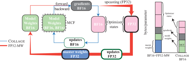
Figure 1: Left: Collage uses a strict low-precision floating-point (such as BF16) optimization loop without ever needing to upcast to FP32 like in the mixed-precision with master weights (red thick loop). The model weights in Collage are represented as multi-component float (MCF) instead of “standard float”. Right: Total bytes/parameter savings for Collage without taking the FP32 upcasting route. The memory savings and uncompromising use of low-precision results in speed-up as seen in Table 7.

We propose Collage , a new approach to deal with floating-point errors in low-precision to make LLM training accurate and efficient. Our primary objective is to develop a training loop with storage strict in low-precision without a need to maintain high-precision clones. We realize that when dealing with low-precision floats (such as Bfloat16), the “standard” representation is not sufficient to avoid rounding errors which should not be ignored. To solve these issues, we rather apply an existing technique of MCF to represent floats which (i) either encounters drastic rounding effects, (ii) the scale of the involved floats has a wide range such that arithmetic operations were lost. We implemented Collage as a plugin to be easily integrated with the well-known optimizers such as AdamW (loshchilov2017decoupled) (extensions to SGD (ruder2017overview) are straight-forward) using low-precision storage & computations. By turning the optimizer to be more precision-aware, even with additional low-precision components in MCF, we obtain faster training (upto $3.7\times$ better train throughput on $6.7$B GPT model, Table 7) and also have less memory foot-print due to strict low-precision floats (see Figure 1 right), compared to the most advanced mixed precision baseline.

We have developed a novel metric called “effective descent quality” to trace the lost information in the optimizer model update step. Due to rounding and lost arithmetic (see definition in Section 3.1), the effective update applied to the model is different from the intended update from optimizer, thus distracting the model training trajectory. Tracing this metric during the training enables to compare different precision strategies at a fine-grained level (see Figure 3 right).

In this work, we answer the critical question of where (which computation) with low-precision during training is severely impacting the performance and why? The main contributions are outlined as follows.

• We provide Collage as a plugin which could be easily integrated with existing optimizer such as AdamW for low-precision training and make it precision-aware by replacing critical floating-points with MCF. This avoids the path of high-precision master-weights and upcasting of variables, achieving memory efficiency (Figure 1 right).

• By proposing the metric effective descent quality, we measure loss in the information at model update step during the training process and provide better understanding of the impact of precisions and interpretation for comparing precision strategies.

• Collage offers wall-clock time speedups by storing all variables in low-precision without upcasting. For GPT-$6.7$B and OpenLLaMA-$7$B, Collage using bfloat16 has up to $3.7\times$ speedup in the training throughput in comparison with mixed-precision strategy with FP$32$ master weights while following a similar training trajectory. The peak memory savings for GPTs ($125$M - $6.7$B) is on average of $22.8\%/14.9\%$ for Collage formations (light/plus), respectively.

• Collage trains accurate models using only low-precision storage compared with FP$32$ master-weights counterpart. For RoBERTa-base, the average GLUE accuracy scores differ by $+0.85\%$ among the best baseline in Table 4. Similarly, for GPT of sizes $125$M, $1.3$B, $2.7$B, $6.7$B, Collage has similar validation perplexity as FP$32$ master weights in Table 5.

2 Background

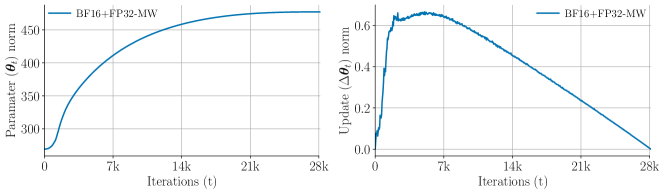
Figure 2: Bert-base-uncased phase-1 pretraining with settings as described in Section 5.1. Left: Model parameter L2 norm vs iterations for BF16 and FP32 master weights strategy. Right: update $\Delta\bm{\theta}_{t}$ L2 norm across iterations. The model parameter norm and update norm are at different scales, for example, $\sim 450$ vs $\sim 0.5$ at $14$k iterations, which is a factor of $900$ and causes lost arithmetic.

We provide a survey on using different floating-points precision strategies for training LLM. We also introduce necessary background information on floating-point representations using a new structure, multi-component float.

2.1 Floats in LLM Training

In LLM training, weights, activation, gradients are usually stored in low precision floating-points such as $16$-bit BF$16$ (micikevicius2017mixed) for enhanced efficiency and optimized memory utilization. The low-bits floating point units (FPUs) are appealing because of its low memory foot-print and computational efficiency. Due to numerical inaccuracies, popular choices of training strategies using FPUs are as follows.

Mixed-precision refers to operations executed in low precision ($16$-bit) with minimal interactions with high precision ($32$-bits) floats, thus offering wall-clock speedups. For example, in GEMM (Generalized Matrix Multiplication), matrix multiplication is performed in 16-bit while accumulation in done in 32-bit through tensor cores in NVIDIA A100 (jia2021A100) and V100 (jia2018dissecting).

Mixed-precision with Master Weights.

Mixed-precision computations of the activations and gradients are not sufficient to ensure a stable training due to encountered numerical inaccuracies, especially, when gradients and model parameters are at different scale, which is the case with large models (see Figure 2 ). A standard workaround is to use the master weight (MW), which refers to maintaining an additional high-precision version (such as $32$-bit float) copy of the model (Figure 1 left) and then performing model update (optimizer step) in high-precision to the master weight (micikevicius2018mixed). To our knowledge, this approach has the state-of-the-art performance among mixed-precision strategies.

Note that, we also use mixed-precision for GEMM (activations and gradients) in our work. In addition to “standard single float” representation which is used in the above strategies, an alternate form is discussed below in Section 2.2.

2.2 Multiple-Component Floating-point

Precise computations can be achieved with one of two approaches in numerical computing.

1. multiple-bit, i.e., using “standard single float” with more bits in the mantissa/fraction, such as 32-, 64-bit floats, and even Bigfloat (granlund2004gnu);

2. multiple-component representation using unevaluated sum $x_{1}+x_{2}+\cdots+x_{n}$ of multiple floats usually in low-precision such as BF$16$, FP$16$, or even FP$8$.

Multiple-bit approach has an advantage of large representation range, while the multiple-component floating-point (MCF) has an advantage in speed, as it consists of only low-precision floating-point computations. Additionally, rounding is often required in $p$-bit “standard single float” arithmetic due to output requiring additional bits to express and store exactly, while in MCF, the rounding error could be circumvent and accounted via appending additional components. A basic structure in MCF is expansion:

Definition 2.1.

(priest1991Arithmetic). A length-$n$ expansion ($x_{1},\ldots,x_{n}$) represents the unevaluated exact sum $x=x_{1}+x_{2}+\cdots+x_{n}$, where components $x_{i}$ are non-overlapping $p$-bit floating-points in decreasing order, i.e., for $i<j$, the least significant non-zero bit of $x_{i}$ is more significant than the most significant non-zero bit of $x_{j}$ or vice versa.

Exact representations of real numbers such as $0.999$ is usually muddled in low-precision, such as BF16, with rounding-to-the-nearest (RN); $0.999\xrightarrow[\text{BF16}]{\text{RN}}1.0$, but can be represented accurately as a length-$2$ expansion $(1.0,-0.001)$ in MCF with two BF$16$ components. The first component serves as an approximation to the value, while the second accounts for the roundoff error. This problem is further aggravated in weighted averaging (see Section 4.2), such that instead of the average, a monotonic increasing sum is produced causing reduced step size and poor learning. We aim to alleviate such problems by using expansions to represent numbers and parameters accurately (e.g., Table 1). Since speed and scalability is critical for LLM training, we are particularly interested in utilizing low-precision MCF (e.g., BF$16$ and FP$16$) as low-bit FPUs are faster than their high-bit counterparts such as FP$32$. For rest of the work, we consider only length-$2$ expansion for MCF as it suffices for our purpose.

3 Imprecision Issues

To motivate the work, in this section, we formalize the issue of imprecision in floating point units. Afterwards, we introduce a novel metric to monitor the information loss. Next, we show its impact via a case study on BERT-like models (devlin2019bert; liu2019roberta). Unless specified otherwise, the low-precision FPU is referred to bfloat$16$, and the same analogy can be easily extended for other low-precision FPUs such as float$16$, float$8$.

3.1 Imprecision with Bfloat16

A commonly encountered problem of computations using low-precision arithmetic is imprecision, where an exact representation of a real-number $x$ either requires more mantissa bits (see Appendix LABEL:appsec:FPU for definitions) beyond the limit (for example, $7$ bits in bfloat$16$), or is not possible (for example, $x=0.1$, is rounded to $0.1001$ in BF16). As a result, the given number $x$ will be rounded to a representable floating-point value, causing numerical quantization errors. An important concept for FPU rounding is unit in the last place ($\operatorname*{ulp}$), which is the spacing between two consecutive representable floating-point numbers, i.e., the value the least significant (rightmost) bit represents if it is $1$.

Definition 3.1 ($\operatorname*{ulp}$ (muller2018handbook)).

In radix $2$ with precision $P$, if $2^{e}\leq|x|<2^{e+1}$ for some integer $e$, then $\operatorname*{ulp}(x)=2^{\max{(e,e_{\min})}-P}$, where $e_{\min}$ is the zero offset in the IEEE 754 standard.

Broadly speaking, two numbers for a given FPU are separated by its $\operatorname*{ulp}$, hence the worst case rounding error for any given $x$ is $\operatorname*{ulp}(x)/2$ (goldberg1991FPU) assumed rounding-to-the-nearest is used. Next, lets denote $\mathcal{F}^{\text{BF16}}(a\,\varkappa\,b)$ as bfloat16 floating-point operation between $a,b$, where $\varkappa$ could be $\oplus$ addition, $\odot$ multiplication, etc. Such operations can be computationally inaccurate and as a consequence, we identify below a problematic behavior with RN.

Definition 3.2 (Lost Arithmetic).

Given the input floating-point numbers $a,b$ and precision $P$. A floating operation $\mathcal{F}^{P}(a\,\varkappa\,b)$ is lost if

$$|\mathcal{F}^{P}(a\,\varkappa\,b)-a|\leq\frac{\operatorname*{ulp}(a)}{2},\,\text{or}\,|\mathcal{F}^{P}(a\,\varkappa\,b)-b|\leq\frac{\operatorname*{ulp}(b)}{2}.$$

Consequently, $\mathcal{F}^{P}(a\,\varkappa\,b)=a,\,\text{or}\,b$, respectively.

Remark: For any non-zero bfloat16 number, if $|b|\leq\text{ulp}(a)/2$, then $\mathcal{F}^{\text{BF16}}(a\,\oplus\,b)=a$. As an example, if $a=200,b=0.1$, then $\mathcal{F}^{\text{BF16}}(200\,\oplus\,0.1)=200$, since $\text{ulp}(200)=1$. Next, we discuss these concepts in the context of LLM training.

3.2 Loss of Information in LLM Training

The situation of ‘adding two numbers at different scale’ is very common in LLM training. See Figure 2 , where due to different scales of model parameter and updates, $\oplus$ in bfloat16 becomes an lost arithmetic. A pseudocode of model parameter ($\bm{\theta}$) update using bfloat16 at iteration $t$ is written as

$$\bm{\theta}_{t}\leftarrow\mathcal{F}^{\text{BF16}}(\bm{\theta}_{t-1}\oplus\Delta\bm{\theta}_{t}),$$ (1)

where, $\Delta\bm{\theta}_{t}$ is the aggregated update from an optimizer (for example, including learning rate, momentum, etc.) at step $t$. With a possibility of lost arithmetic in Equation (1), the actual updated parameter could be different from expected. Hence, we define the effective update at step $t$ as

$$\widehat{\Delta\bm{\theta}}_{t}=\mathcal{F}^{\text{BF16}}(\bm{\theta}_{t-1}\oplus\Delta\bm{\theta}_{t})-\bm{\theta}_{t-1}.$$ (2)

Note that in the event of no lost arithmetic, $\widehat{\Delta\bm{\theta}}_{t}=\Delta\bm{\theta}_{t}$. While, when $\widehat{\Delta\bm{\theta}}_{t}\neq\Delta\bm{\theta}_{t}$ which is usually the case with low-precision FPUs, there is a loss in information as $\leq\operatorname*{ulp}/2$ values are simply ignored (see Figure 3). To better capture this information loss, we introduce a novel metric.

Definition 3.3 (Effective Descent Quality).

Given the current parameter, aggregated update at step $t$ as $\bm{\theta}_{t}$, $\Delta\bm{\theta}_{t}$, respectively. The effective descent quality for a given floating-pint precision is defined as

$$\operatorname*{EDQ}(\Delta\bm{\theta}_{t},\widehat{\Delta\bm{\theta}}_{t};\bm{\theta}_{t},P)=\Big{\langle}\frac{\Delta\bm{\theta}_{t}}{||\Delta\bm{\theta}_{t}||},\widehat{\Delta\bm{\theta}}_{t}\Big{\rangle},$$ (3)

where, $\widehat{\Delta\bm{\theta}}_{t}$ is defined in eq. (2) for a given precision $P$.

In other words, $\operatorname*{EDQ}$ in eq. (3) is projection of the effective update along the desired update. In the absence of any imprecision, $\operatorname*{EDQ}$ will be simply the norm of original update. We show in Section 5.1 and Figure 3 how $\operatorname*{EDQ}$ relates to the learning and helps understanding impacts of different precision strategies.

To remedy the imprecision and lost arithmetic in the model parameter update step (Equation (1)), works such as Kahan summation (zamirai2020revisiting; park2018training) exist (see Appendix LABEL:app-para:kahan), however, we see in Figure 3 (Middle) that although Kahan-based BF$16$ approach improves over ‘BF$16$’ training but it still could not match with the commonly used FP$32$ master weights approach.

4 Collage: Low-Precision MCF Optimizer

In this section, we present Collage, a low precision strategy & optimizer implementation to solve aforementioned imprecision and lost arithmetic issues in Section 3 without upcasting to a higher precision, using the multiple-component floating-point (MCF) structure.

4.1 Computing with MCF

Precise computing with exact numbers stored as MCF expansions is easy with some basic algorithms. For example, Fast2Sum captures the roundoff error for the float addition $\oplus$ and outputs an expansion of length $2$.

Theorem 4.1 (Fast2Sum (dekker1971float)).

Let two floating-point numbers $a,b$ be $|a|\geq|b|$, Fast2Sum produces a MCF expansion $(x,y)$ such that $a+b=x+y$, where $x\leftarrow\mathcal{F}^{P}(a\oplus b)$ is the floating-point sum with precision $P$, $y\leftarrow\mathcal{F}^{P}\left(b\ominus\mathcal{F}^{P}(x\ominus a)\right)=a+b-\mathcal{F}^{P}(a\oplus b)$ is the rounding error. Also, $y$ is upper-bounded such that $|y|<\operatorname*{ulp}(x)/2$.

Algorithm 2 Collage: Bfloat$16$ MCF AdamW Optimization

1:  Given $\alpha$ (learning rate), $\beta_{1}$, $\beta_{2}$, $\epsilon$, $\lambda\in\mathbb{R}$

2:  Initialize time step: $t\leftarrow 0$, BF$16$ parameter vector $\bm{\theta}_{t=0}\in\mathbb{R}^{n}$, BF$16$ first moment vector: $\bm{m}_{t=0}\leftarrow\bm{0}$, BF$16$ second moment vector: $\bm{v}_{t=0}\leftarrow\bm{0}$

3:  Initialize 2nd component $\bm{\delta\theta}_{t=0}\leftarrow\bm{0}$ in BF$16$ for parameter

4:  (optional) Represent $\beta_{2}$ as expansion $(\hat{\beta}_{2},\delta\beta_{2})$, initialize 2nd component $\bm{\delta v}_{t=0}\!\leftarrow\!\bm{0}$ in BF$16$ for second moment

5:  repeat

6:     $t\leftarrow t+1$

7:     $\bm{g}_{t}\leftarrow\nabla f_{t}(\bm{\theta}_{t-1})$

8:     $\bm{m}_{t}\leftarrow\beta_{1}\cdot\bm{m}_{t-1}+(1-\beta_{1})\cdot\bm{g}_{t}$

9:     $\bm{v}_{t}\leftarrow\beta_{2}\cdot\bm{v}_{t-1}+(1-\beta_{2})\cdot\bm{g}_{t}^{2}$     $\Longrightarrow~{}~{}~{}~{}(\bm{v}_{t},\bm{\delta v}_{t})\leftarrow\textbf{Grow}(\textbf{Mul}(\hat{\beta}_{2},\delta\beta_{2}),(\bm{v}_{t-1},\bm{\delta v}_{t-1})),(1-\beta_{2})\cdot\bm{g}_{t}^{2})$

10:     $\hat{\bm{m}}_{t}\leftarrow\bm{m}_{t}/(1-\beta_{1}^{t})$

11:     $\hat{\bm{v}}_{t}\leftarrow\bm{v}_{t}/(1-\beta_{2}^{t})$

12:     $\bm{\Delta\theta}_{t}\leftarrow-\alpha(\hat{\bm{m}}_{t}/(\sqrt{\hat{\bm{v}}_{t}+\epsilon})+\lambda\bm{\theta}_{t-1})$

13:     $\bm{\theta}_{t}\leftarrow\bm{\theta}_{t-1}+\bm{\Delta\theta}_{t}$     $\Longrightarrow~{}~{}~{}~{}(\bm{\theta}_{t},\bm{\delta\theta}_{t})\leftarrow\textbf{Grow}((\bm{\theta}_{t-1},\bm{\delta\theta}_{t-1}),\bm{\Delta\theta}_{t})$

14:  until stopping criterion is met

15:  return: optimized parameters $\bm{\theta}_{t}$

Note that, particularly for LLM training, we are able to add using Fast2Sum without any sorting since parameter weights $\bm{\theta}$ are usually larger than the gradients and updates $\bm{\Delta\theta}$ in absolute value at the parameter update step Equation (1) (See Figure 2 ). Similar basic algorithms exist for the multiplication of two floats, which produces in the same way a length-2 expansion. Using the basic algorithms, an exhaustive set of advanced algorithms are developed (yu2022mctensor). We refer the reader to Appendix LABEL:appsec:mcf_algs for more details. Particularly, for the optimizer update step (1), a useful algorithm to introduce is Grow (see Algorithm 1) which adds a float to a MCF expansion of length $2$.

Algorithm 1 Grow

1:  Input: an expansion $(x,y)$ and a float $a$ with $|x|\geq|a|$

2:  $(u,v)\leftarrow\textbf{Fast2Sum}(x,a)$

3:  $(u,v)\leftarrow\textbf{Fast2Sum}(u,y+v)$

4:  Return: $(u,v)$

4.2 Collage: Bfloat$16$ MCF AdamW

Using the basic components from Section 4.1 and Appendix LABEL:appsec:mcf_algs, we now provide plugins to modify a given optimizer such as AdamW (loshchilov2017decoupled) to be precision-aware and store entirely with low-precision floats, specifically bfloat$16$ in Algorithm 2. Note that, mixed-precision is still used in GEMM for obtaining gradients and activations but are stored in bfloat$16$ only. The required changes are highlighted in pink, and are discussed individually as follows.

Model Parameters

We substitute the bfloat$16$ model parameter $\bm{\theta}_{t}$ with a length-$2$ MCF expansion $(\bm{\theta}_{t},\bm{\delta\theta}_{t})$ by appending an additional bfloat$16$ variable $\bm{\delta\theta}_{t}$ in line-$3$ which does not require any gradients. Next, to update the model parameter expansion, we use Grow in line-13 to add a float $\Delta\bm{\theta}_{t}$ to the expansion.

Table 1: length-$2$ expansions for $\beta_{2}$ in Bfloat$16$.

$\beta_{2}$	BF$16$ MCF
$0.999$	$(1,-0.001)$
$0.99$	$(0.9893,0.0017)$
$0.95$	$(0.9492,0.0008)$

Optimizer States

With Adam-like algorithms, unlike the first moment $\bm{m}_{t}$, the second moment $\bm{v}_{t}$ update suffers from severe imprecision and lost arithmetic due to smaller accumulation, $\bm{g}_{t}$ vs $\bm{g}_{t}^{2}$. To make the matter worse, default choice of $\beta_{2}$ such as $0.999$ (devlin2019bert) are simply rounded to $1.0$ in bfloat$16$, thus resulting in a monotonic increase in second momentum. This in turn makes the update $\Delta\bm{\theta}_{t}$ smaller and hence slower learning as we see in Figure 3. To alleviate this issue, we propose switching $\beta_{2}$ from standard single float to a MCF expansion as $(\beta_{2},\delta\beta_{2})$, and also for second momentum as $(\bm{v}_{t},\bm{\delta v}_{t})$. Doing so, we have an exact representation of $\beta_{2}$ as shown in Table 1. We then perform a multiplication of two expansions using Mul (see Appendix LABEL:appsec:mcf_algs).

Table 2: Precision breakdown of various training strategies applied to the given optimizer. The strategies are ranked from top to bottom in the order of byte/parameter occupancy.

Precision Option	Stages & Components			Memory (bytes/parameter)
	Parameter & Gradient	Optimizer States	MCF or Master Weight
A (BF$16$)	BF$16\times 2$	BF$16\times 2$	NA	$8$
B (Collage-light) (ours)	BF$16\times 2$	BF$16\times 2$	BF$16\times 1$	$10$
C (Collage-plus) (ours)	BF$16\times 2$	BF$16\times 2$	BF$16\times 2$	$12$
D (BF$16$ + FP$32$Optim + FP$32$MW)	BF$16\times 2$	FP$32\times 2$	FP$32\times 1$	$16$

For the sake of simplicity in notations, we denote Collage-light as using MCF expansions only for model parameters and Collage-plus for both model parameters and optimizer states. It’s worthy to note that imprecision and lost arithmetic are common and sometimes hard to notice. We only identify places when they hurt training accuracies. A rule of thumb is to do as many scalar computations in high precision as possible before casting them to low precision (e.g., PyTorch BFloat$16$ Tensor). Worthy to note, existing Kahan-based optimizers are special cases of Collage-light under a magnitude assumption, we defer this discussion and other places of imprecision and lost arithmetic such as weight decay that exist in the algorithm to Appendix LABEL:appsec:further_discussions_algorithm.

Table 3: Pre-training perplexity of BERT (both phases) and RoBERTa for all precision strategies as listed in Table 2. Lower values are better, with the best results in bold. D${}^{-\text{MW}}$ with FP$32$Optim with same bytes/parameter as Collage could not match its performance.

Precision Option	$\beta_{2}=0.999$				$\beta_{2}=0.98$
	BERT-base		BERT-large		RoBERTa-base
	Phase-$1$	Phase-$2$	Phase-$1$	Phase-$2$
A	$8.67$	$7.61$	$6.05$	$5.47$	$3.82$
B (Collage-light)	$5.99$	$5.26$	$4.39$	$3.90$	$3.49$
C (Collage-plus)	$\bf{5.26}$	$\bf{4.66}$	$\bf{3.94}$	$\bf{3.53}$	$3.49$
D${}^{-\text{MW}}$ (BF$16$ + FP$32$Optim)	$6.23$	$5.64$	$4.66$	$4.22$	$3.82$
D	$\bf{5.26}$	${4.71}$	$4.06$	$3.63$	$\bf{3.46}$

5 Empirical Evaluation

We evaluate Collage formations against the existing precision strategies on pretraining LLMs at different scales, including BERT (devlin2019bert), RoBERTa (liu2019roberta), GPT (gpt-neox-library), and OpenLLaMA (touvron2023llama). Specifically, we compared the following precision strategies in our experiments, which are ordered in an increasing number of byte/parameter (see Table 2).

• Option A: Bfloat$16$ parameters

• Option B: Bfloat$16$ + Collage-light

• Option C: Bfloat$16$ + Collage-plus

• Option D: Bfloat$16$ + FP$32$ Optimizer states + FP$32$ master weights

Since option D is the best-known baseline with state-of-the-art quality among mixed-precision strategies, we aim to outperform, or at least match the quality of option D with Collage throughout our experiments. We show that Collage matching the quality of option D, has orders-magnitude higher performance (speed, see Table 7). All strategies are evaluated using AdamW (loshchilov2017decoupled) optimizer with standard $\beta_{1}=0.9$ while varying $\beta_{2}$ as per different experiments. We use aws.p4.24xlarge compute instances for all of our experiments.

5.1 Pre-training BERT & RoBERTa

We demonstrate that BF$16$-Collage can be used to obtain an accurate model, comparable to heavy-weighted FP$32$ master weights strategy.

Precision options.

In addition to options A, B, C, D, we further augment our experiments with another baseline strategy D${}^{-\text{MW}}$, where we disabled the FP$32$ master weights but only used FP$32$ optimizer states. This strategy saves $4$ bytes/parameter in comparison to Option D and has the same bytes/parameter as option C (Collage-plus).

Model and Dataset.

We first pre-train the BERT-base-uncased, BERT-large-uncased, and RoBERTa-base model with HuggingFace (HF) (wolf2019huggingface) configuration on the Wikipedia-en corpus (Wikiextractor2015), preprocessed with BERT Wordpiece tokenizer. We execute the following pipeline to pretrain, i) BERT in two phases with phase-1 on $128$ sequence length, and then phase-2 with $512$ sequence length; and ii) RoBERTa with sequence length $512$. We adopt $\beta_{2}=0.999$ for BERT and $\beta_{2}=0.98$ for RoBERTa following the configs from HF. We defer more training details to Appendix LABEL:appssec:bert_roberta.

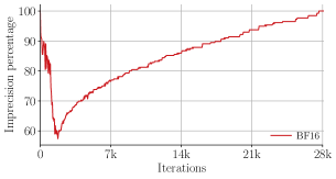
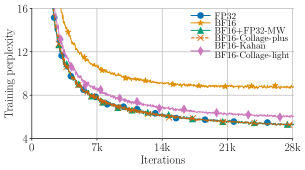
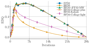
Figure 3: BERT phase-$1$ pre-training (see Appendix LABEL:appssec:bert_roberta for details). Left: Imprecision percentage ($\%$) measured as the percentage of lost arithmetic for all model parameters, i.e., not updated, vs iterations for BF$16$. Middle: Training perplexity vs iterations for various precision strategies (see Table 2). Additionally, we evaluate “FP32” as 32-bit counterpart of option A, and BF16-Kahan as Kahan-sum (zamirai2020revisiting) with BF16 parameters. Right: Effective descent quality ($\operatorname*{EDQ}$) in (3) vs iterations to measure loss in information at the optimizer step for different precision strategies. BF16-Collage-plus training perplexity and $\operatorname*{EDQ}$ overlaps with the best “FP32”, and “BF16 + FP32 MW” with less bytes/parameter.

Table 4: GLUE benchmark for BERT-base-uncased and RoBERTa-base pre-trained using different precision strategies. See Appendix LABEL:appssec:bert_roberta for experimental details. BF$16$-Collage training strategy matches/exceeds the finetuning quality over several metrics.

Model	Precision	MRPC	QNLI	SST-2	CoLA	RTE	STS-B	QQP	MNLI	Avg
BERT-base	A	$0.8210$	$0.8832$	$0.8890$	$0.3522$	$0.6462$	$0.8666/0.8618$	$0.8973$	$0.7993$	$0.7796$
	B (ours)	$0.8431$	$0.8974$	$0.9071$	$0.4149$	$0.6606$	$0.8837/0.8785$	$0.9031$	$0.8184$	$0.8007$
	C (ours)	$0.8602$	$\bf{0.9090}$	$\bf{0.9128}$	$\bf{0.4314}$	$0.6698$	$0.8851/0.8821$	$\bf{0.9069}$	$\bf{0.8330}$	$\bf{0.8100}$
	D	$\bf{0.8651}$	$0.9071$	$0.9036$	${0.4212}$	$\bf{0.6714}$	$\bf{0.8890/0.8849}$	${0.9064}$	$\bf{0.8330}$	${0.8090}$
RoBERTa-base	A	${0.8504}$	$0.8914$	$0.9000$	$0.3866$	${0.6281}$	$0.8636/0.8625$	$0.8981$	$0.8155$	$0.7884$
	B (ours)	$0.8455$	${0.9000}$	${0.9025}$	${0.4460}$	${0.6281}$	${0.8636/0.8635}$	${0.9002}$	$0.8182$	${0.7964}$
	C (ours)	$\bf{0.8529}$	$\bf{0.9040}$	$\bf{0.9048}$	$\bf{0.4588}$	$0.6137$	$\bf{0.8658/0.8647}$	$\bf{0.9005}$	$\bf{0.8230}$	$\bf{0.7986}$
	D	$0.8406$	$0.8993$	$0.9002$	$0.3870$	$\bf{0.6389}$	$0.8622/0.8631$	$0.8999$	${0.8203}$	$0.7901$

Results.

The final pretraining perplexity of various precision strategies are summarized in Table 3 and for BERT-base, the complete phase-$1$ training loss trajectory is shown in Figure 3 middle. Additionally, we did finetuning of the pre-trained models on the GLUE benchmark (wang2019glue) for eight tasks in Table 4 with the same configurations specified in Appendix LABEL:appssec:bert_roberta. Collage-plus although using only BF16 parameters, outperforms the vanilla BF16 option A and matches/exceeds option D for both pre-training and finetuning experiments. For BERT-base Collage-plus exceeds on 5/8 tasks with $+0.1\%$ lead in average, while for roberta-base its exceeds on 7/8 tasks with $+0.85\%$ in average. Note that, although D${}^{-\text{MW}}$ has FP$32$ optimizer states and same/more byte/parameter complexity as Collage-plus/light, respectively, it could not match the quality showing the importance of MCF in the AdamW through Collage. This shows that simply having higher-precision is not enough to obtain better models but requires a careful consideration of the floating errors.

Interestingly, Collage-light suffices to closely match the option D in the RoBERTa pretraining experiments with $\beta_{2}=0.98$, while lagging to match with the $\beta_{2}=0.999$ BERT pretraining experiments. Our proposed metric, the effective descent quality ($\operatorname*{EDQ}$) provides a nuanced understanding of this phenomenon in Figure 3 (Right). Collage-light and Kahan-based approach improve $\operatorname*{EDQ}$ upon BF$16$ option A at the parameter update step, yet cannot achieve the optimal $\operatorname*{EDQ}$ due to lost arithmetic at the exponential moving averaging step. In contrast, Collage-plus achieves better $\operatorname*{EDQ}$ by taking it into considerations and thereby outperforms the best-known baseline, Option D.

5.2 Pretraining multi-size GPTs & OpenLLaMA 7B

Model and Dataset.

We conduct following pretraining experiments; 1) GPT with different sizes ranging from $125$M, $1.3$B, $2.7$B to $6.7$B, and 2) OpenLLaMA-$7$B using NeMo Megatron (kuchaiev2019nemo) with the provided configs. The GPTs are trained on the Wikipedia corpus (Wikiextractor2015) with GPT$2$ BPE tokenizer, and OpenLLaMA-$7$B on the LLaMA tokenizer, respectively. Additional training and hyerparameter details are described in Appendix LABEL:appssec:gpt_llama.

Results.

Using the recommended $\beta_{2}=0.95$ (gpt-neox-library), Table 5 summarizes the train & validation perplexity after pre-training GPT models and OpenLLaMA-$7$B under various options. Our Collage formations are able to match the quality of the best-known baseline, FP$32$ MW option D, most of the time for all models with the only exception on the smallest GPT-$125$M, while having the same validation perplexity.

Table 5: Left: Train $|$ Validation perplexity of pre-trained GPT with $\beta_{2}=0.95$. Right: OpenLLaMA-$7$B with $\beta_{2}=0.95$ and $0.99$.

Model	GPT
Precision Option	$125$M	$1.3$B	$2.7$B	$6.7$B
A (BF16)	$14.73~{}|~{}15.64$	$10.28~{}|~{}12.43$	$9.97~{}|~{}12.18$	$9.87~{}|~{}12.18$
B (Collage-light)	$14.01~{}|~{}15.03$	$8.50~{}|~{}17.70$	$8.33~{}|~{}11.36$	$8.17~{}|~{}11.13$
C (Collage-plus)	$14.01~{}|~{}15.03$	$8.50~{}|~{}17.70$	$8.33~{}|~{}11.36$	$8.17~{}|~{}11.13$
D (BF$16$ + FP$32$Optim + FP$32$MW)	$13.87~{}|~{}15.03$	$8.50~{}|~{}17.70$	$8.33~{}|~{}11.36$	$8.17~{}|~{}11.13$

OpenLLaMA-7B
$\beta_{2}=0.95$	$\beta_{2}=0.99$
$6.36~{}|~{}4.81$	$15.96~{}|~{}12.55$
$5.99~{}|~{}4.53$	$8.00~{}|~{}5.99$
$5.99~{}|~{}4.57$	${6.11~{}|~{}4.62}$
$5.99~{}|~{}4.57$	$8.58~{}|~{}6.42$

Table 6: Train $|$ Validation perplexity of GPT-$125$M pre-trained with $\beta_{2}\in\{0.95,0.99,0.999\}$ and Global BatchSize $\in\{1024,2048\}$.

Precision Option	Global BatchSize $=1024$			Global BatchSize $=2048$
	$\beta_{2}=0.95$	$\beta_{2}=0.99$	$\beta_{2}=0.999$	$\beta_{2}=0.95$	$\beta_{2}=0.99$	$\beta_{2}=0.999$
A (BF16)	$14.73~{}|~{}15.64$	$14.88~{}|~{}15.80$	$17.29~{}|~{}18.17$	$14.73~{}|~{}15.18$	$14.88~{}|~{}15.33$	$17.64~{}|~{}15.33$
B (Collage-light)	$14.01~{}|~{}15.03$	$14.01~{}|~{}15.03$	$14.88~{}|~{}15.80$	$13.87~{}|~{}14.44$	$13.87~{}|~{}14.44$	$14.59~{}|~{}15.18$
C (Collage-plus)	$14.01~{}|~{}15.03$	$14.01~{}|~{}15.03$	$14.15~{}|~{}15.18$	$13.87~{}|~{}14.44$	$13.87~{}|~{}14.44$	$14.01~{}|~{}14.59$
D (BF$16$ + FP$32$Optim + FP$32$MW)	$13.87~{}|~{}15.03$	$14.01~{}|~{}15.03$	$14.01~{}|~{}15.03$	$13.87~{}|~{}14.44$	$13.87~{}|~{}14.44$	$14.01~{}|~{}14.59$

Ablation: Impact of $\beta_{2}$.

We conduct ablation experiments to illustrate the impact of $\beta_{2}$ on the quality of precision strategies by further pre-training the GPT-$125$M model using $\beta_{2}=0.99$ and $0.999$, with a global batchsize $1024$, $2048$ and the same micro-batchsize $16$, as summarized in Table 6. Similar to the BERT and RoBERTa pre-training experiments, Collage-light is able to closely match Option D when $\beta_{2}=0.95$ or $0.99$ and remain unaffected by changes in the global batchsize.

However, with $\beta_{2}=0.999$, Collage-light underperforms option D while Collage-plus is still able to closely match option D. As analyzed in Section 4.2, low precision (Bfloat$16$) arithmetic fails to represent and compute with $\beta_{2}=0.999$ due to rounding errors. In fact, we observed the same phenomenon as pre-training BERT & RoBERTa in Section 5.1, including i) a high imprecision percentage of lost additions with low-precision BF$16$ arithmetic; ii) a reduced $\operatorname*{EDQ}$ for Collage-light and a better $\operatorname*{EDQ}$ for Collage-plus. These together rationalize the utility and significance of our proposed metric $\operatorname*{EDQ}$ and the necessity of Collage-plus for quality models. We defer figures of these metrics for GPTs to Appendix LABEL:appssec:gpt_pt.

We also pretrain OpenLLaMA-$7$B with $\beta_{2}=0.99$ in Table 5 (right), where both Collage formations outperform option D. In fact, we observe that $\beta_{2}=0.99$ can easily lead to gradient explosion (see Figure LABEL:fig:openllama-7B-beta2_0p99 right in Appendix LABEL:appssec:openllama7B_pt), while Collage-plus provides stable training. The training perplexity trajectories in Figure LABEL:fig:openllama-7B-beta2_0p95,LABEL:fig:openllama-7B-beta2_0p99 (in Appendix LABEL:appssec:openllama7B_pt) show that Collage-plus effectively solves the imprecision issue and produces quality models.

Remark 5.1.

The optimal choice of $\beta_{2}$ differs case-by-case. To our best knowledge, there is no clear conclusion between $\beta_{2}$ and the converged performance of the pre-trained models. Showing Collage works with different $\beta_{2}$’s, enable LLM training to be not limited by such precision issues.

5.3 Performance and Memory

Throughput.

We record the mean training throughput of precision strategies for pre-training GPTs and OpenLLaMA-$7$B in a simple setting for fair comparisons: one aws.p4.24xlarge node with sequence parallel (korthikanti2023reducing) turned off, and present relative speed-up in Table 7. Both Collage formations are able to maintain the efficiency of option A. Moreover, the speed factor for Collage increases with an increase in the model size, obtaining up to $\bm{3.74\times}$ for GPT-$6.7$B model.

Table 7: Relative speed-up compared to the option D.

Precision	GPT			OpenLlama $7$B
Option	$1.3$B	$2.7$B	$6.7$B
A	1.78$\times$	2.59$\times$	3.82$\times$	3.15$\times$
B (ours)	1.74$\times$	2.57$\times$	3.74$\times$	3.14$\times$
C (ours)	1.67$\times$	2.48$\times$	3.57$\times$	3.05$\times$
D	1$\times$	1$\times$	1$\times$	1$\times$

Memory.

We probe the peak GPU memory of all training precision strategies during practical runs on $8\times$NVIDIA A$100$s ($40$GB) with the same hyper-parameters for a fair comparison: sequence length $2048$, global batchsize $128$ and micro (per-device) batchsize $1$. Figure 4 visualizes the peak memory usage of GPTs vs model sizes. During real runs, on average, Collage formations (light/plus) use $23.8\%/15.6\%$ less peak memory compared to option D. The best savings are for the largest model OpenLLaMA-$7$B, with savings $27.8\%/18.5\%$, respectively.

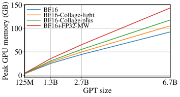
Figure 4: GPU peak memory in GB vs model size. GPT-$125$M is hosted on $1$ NVIDIA A$100$ $40$GB, while all other models were hosted on $8\times$ A$100$ $40$GB using tensor-parallelism $8$.

Increased Sequence Length and Micro BatchSize.

Table 8: Memory compatibility of pre-training GPT-NeoX-$30$B using precision options with different micro batchsize (UBS) and sequence length.

Precision	UBS$=1$		UBS$=2$
option   /   SeqLen	$1,024$	$2,048$	$1,024$	$2,048$
A (BF$16$)	$\checkmark$	$\checkmark$	$\checkmark$	$\checkmark$
B (Collage-light)	$\checkmark$	$\checkmark$	$\checkmark$	$\operatorname*{OOM}$
C (Collage-plus)	$\checkmark$	$\checkmark$	$\checkmark$	$\operatorname*{OOM}$
D (BF$16$ + FP$32$Optim + FP$32$MW)	$\checkmark$	$\operatorname*{OOM}$	$\operatorname*{OOM}$	$\operatorname*{OOM}$

We study the benefits of Collage’s reduced memory foot-print (as shown in Figure 4), with a demonstration on pre-training a large GPT-$30$B model with tensor-parallelism=$8$, pipeline-parallelism=$2$ on two aws.p4.24xlarge ($8\times$A100s $40$GB) instances. Specifically, we identify the maximum sequence length and micro batchsize for all precision strategies to be able to run without $\operatorname*{OOM}$, as summarized in Table 8. Collage enables training with an increased sequence length and micro batchsize compared to option D, thus providing a smooth trade-off between quality and performance.