Network analysis for the steady-state thermodynamic uncertainty relation
Abstract
We perform network analysis of a system described by the master equation to estimate the lower bound of the steady-state current noise, starting from the level 2.5 large deviation function and using the graph theory approach. When the transition rates are uniform, and the system is driven to a non-equilibrium steady state by unidirectional transitions, we derive a noise lower bound, which accounts for fluctuations of sojourn times at all states and is expressed using mesh currents. This bound is applied to the uncertainty in the signal-to-noise ratio of the fluctuating computation time of a schematic Brownian computation plus reset process described by a graph containing one cycle. Unlike the mixed and pseudo-entropy bounds that increase logarithmically with the length of the intended computation path, this bound depends on the number of extraneous predecessors and thus captures the logical irreversibility.
I Introduction
The thermodynamic uncertainty relation (TUR) provides a universal trade-off between precision and dissipation [1]. In the last decade, the TUR and its relatives—the trade-off relation and speed limits—have been discussed from various perspectives, e.g., Ref. [2]. Among these, the TUR has been applied to Bayes nets [3] and Brownian computation models [4]. Such networks, typically large-scale, possess information processing capabilities, making them intriguing subjects from novel aspects of the thermodynamics of computation [5, 6]. However, the TUR bound is anticipated to be weak for large networks because it is formulated in quantities, such as entropy production and activities, that increase as the system size grows. Therefore, tightening the bound is necessary for the practical application of TUR to computation models extended to include dynamics.
Graph theory is a well-established tool for analyzing electric circuit networks [7, 8, 9, 10]. The network is algebraically treated using the circuit matrices, i.e., the incidence matrix, the cycle (loop) matrix, and the cutset matrix. This approach aims to systematically reduce the number of free coordinates in the circuit equations or Lagrangians [10]. In the present paper, we perform a network analysis of a directed multigraph describing a Markov chain in the steady state. Such a graph can describe the Brownian computation plus reset process [4, 11].
For this purpose, we go back to the level 2.5 large deviation function adopted in early TUR studies [12, 13, 14, 15, 16, 17, 18, 19, 20]. The level 2.5 large deviation function provides the joint probability distribution of the numbers of jumps at all arcs and the sojourn times at all nodes in the limit of long measurement time. It derives a formally exact expression of the probability distribution of steady-state current, thus serving as a solid starting point for the network analysis. We derive a lower bound of the current noise when considering both bidirectional and unidirectional transition processes with uniform transition rates. The importance of network topology has been recognized in the studies of the steady-state TUR [16, 17, 18] and the level 2.5 large deviation theory [12, 13] in connection to the steady-state fluctuation theorem [21]. These studies have focused on the universal aspect, while in the present paper, we emphasize practical application to large networks, especially to the Brownian computation model.
A secondary purpose of the paper is to provide an elementary derivation of the level 2.5 large deviation function based on the full-counting statistics (FCS) [22, 23]. The original derivation is rigorous and intricate [12, 13]. We aim for our derivation to be an accessible introduction to this concept for the mesoscopic quantum transport community and to make this paper self-contained simultaneously.
The structure of the paper is as follows: In Sec. II, we re-derive the level 2.5 large deviation function using the FCS approach and summarize previously known noise lower bounds. This section also introduces notations, which we use for our graph theoretical analysis. Section III explains our contributions: After introducing the circuit matrices, we derive a lower bound of current noise by duality transformation for systems with uniform transition rates. In Sec. IV, we apply our bound to a schematic Brownian computation model. Section V summarizes our results.
II level 2.5 rate function and TUR
II.1 FCS approach
The state transition diagram of a continuous-time Markov chain is a directed multigraph , where the set of nodes and the set of arcs (directed edges) represent states and transitions, respectively. We focus on a connected graph with a unique steady state for simplicity. The direction of an arc corresponds to the direction of a transition. We write the arc from the tail node to the head node as a tuple . The boundary operator maps the arc to the node as . The positive (negative) incidence matrix is defined as, . The incidence matrix is . We denote the reversed arc of as , which satisfies, . The master equation is,
| (1) | ||||
| (2) |
where is the state probability of node , and is the transition rate associated to arc .
We introduce the number of transitions through each arc in its direction, , and the sojourn time at each node , . Their joint probability distribution function during the measurement time is,
| (3) |
where and are the counting fields for currents [22] and dwell times [23]. In the limit of long measurement time , , where is the eigenvalue of the modified (tilted) transition rate matrix,
| (4) |
with the maximum real part. Then, within the saddle point approximation, , where the rate function is,
| (5) |
The flux and the node state probability satisfy the Kirchhoff current law (KCL) and the normalization condition, respectively:
| (6) | ||||
| (7) |
We introduce the orthonormalized right and left eigenvectors associated with the eigenvalue as,
| (8) |
By noticing that and are orthonormalized and are the functions of and , the change of eigenvalue induced by small variations and is calculated as, . By using this we find that the maximum in Eq. (5) is achieved when and implicitly fulfill,
| (9) |
By substituting these solutions into Eq. (5) and using the KCL (6), we obtain the level 2.5 large deviation function:
| (10) | ||||
| (11) |
II.2 Bidirectional and unidirectional processes
The set of arcs is partitioned into mutually disjoint sets of arcs for unidirectional transitions and bidirectional transitions as and . The set for bidirectional transitions is further partitioned into the sets for forward transitions and backward transitions as and . Here and hereafter, we use the overline to represent the set of reversed arcs, . In the following, we limit ourselves to the case that there exists so that an oriented graph contains a directed rooted spanning tree, . For , we introduce anti-symmetrized and symmetrized fluxes, and , and integrate out the latter,
| (12) |
This can be done (see e.g. Ref. [18]) and the result is,
| (13) | ||||
| (14) |
Here we write for and introduced, . The KCL (6) for the edge current becomes,
| (15) |
The steady-state edge current , where is the node state probability in the steady-state, satisfies the KCL. The rate function (13) takes the maximum at and as .
II.3 Mixed and pseudo-entropy bounds
We are interested in the probability distribution of the weighted sum of the edge currents,
| (17) |
which is obtained by contraction,
| (18) |
subjected to the constraints (7), (15) and (17). The rate function takes the maximum at the average .
We introduce a parameter representing the deviation from the average, . Then by substituting and to Eq. (18) and by using the inequalities [15], and (Appendix A),
| (19) |
we obtain the mixed bound [27, 28]:
| (20) | ||||
| (21) |
where is the cubic and quartic terms of the right-hand side of Eq. (19). Equation (20) applies to all cumulants.
In the following, we focus on the second cumulant and utilize edge current and state probability vectors for concise presentations. We refer to as the cotree of , which contains arcs not in , and . Hereafter, the number of elements of a set is denoted as . The edge current vector is an component real vector. Here and are defined on twigs (arcs of the directed rooted spanning tree ) and on chords (arcs of the cotree ) , respectively. The state probability vector is , where, .
A small deviation shifts the maximizing parameters as,
| (22) | ||||
| (23) |
By substituting them into Eq. (18) and expanding up to second order in , we obtain, , where [29],
| (24) |
The inverse of diagonal weight matrix is and . Here and hereafter, we set for . The constraints (7), (15) and (17) are,
| (25) | ||||
| (26) |
where , and is a real vector whose entries are 1s.
III Lower bound of current noise
III.1 Circuit matrices
We summarize circuit matrices relevant to our network analysis (see, e.g., Refs. [7, 8] and Appendices of Ref. [10]). We write a fundamental cycle of length as a tuple, a sequence of one chord and twigs or reversed ones :
| (28) |
The head and tail of adjacent arcs, and , () share the same node . The first and last arcs satisfy the periodic boundary condition . The fundamental cycle matrix indicates which arcs are included in each of fundamental cycles:
| (29) |
where is a unit matrix and ,
| (30) |
for and . The indicator function equals if and equals if .
There is a unique directed path from the root to a node along the directed rooted spanning tree , which we write as a sequence of twigs as,
| (31) |
Here is the length of the path. Similar to the cycle, the head and tail of adjacent arcs share the same node. The two endpoints are and . We introduce a root-to-node path matrix as a variant of the node-to-datum path matrix [7, 8, 9],
| (32) |
which is 1(0) if a twig is in (not in) the path from the root to the node . The fundamental cutset matrix is then introduced as (Appendix B),
| (33) |
which implies that acts as the line integral along the directed rooted spanning tree. The fundamental cutset is a minimal set of arcs consisting of one twig and zero or more chords that is the boundary of two regions. Its component is () if an arc is in the fundamental cutset with respect to the twig and bridges the two regions in the same (opposite) direction of the twig .
The incidence matrix and the cycle matrix satisfy (Appendix B),
| (34) | ||||
| (35) |
where, for example, is a zero matrix. The cutset matrix satisfies similar relations:
| (36) | ||||
| (37) |
Equalities (34), (35), (36) and (37) indicates,
| (38) | ||||
| (39) |
The first (second) inclusion relation corresponds to that between groups of (co)boundaries and (co)cycles [30]. Intuitively, Eqs. (35) and (37) correspond to in the vector analysis.
III.2 Duality transformation
In the following, we limit ourselves to the uniform transition rates,
| (40) |
In this case, the unidirectional transitions drive the system out of equilibrium. In Eq. (24), can be separated into the ‘curl-free’ component and the source term coming from the unidirectional transitions:
| (41) |
where is a unit vector, . One can check , where , satisfies the constraint (26). By substituting it into Eq. (41), we obtain,
| (42) | ||||
| (43) |
where is,
| (44) |
Here, is a subtree rooted at obtained by cutting the directed rooted spanning tree by removing the arc . The number of nodes in this subtree is . For explicit form of , see Appendix C.
We perform the duality transformation [31], which is in the present context, integrating out the ‘curl-free’ component by introducing the auxiliary field to Eq. (24) as,
| (45) | ||||
| (46) |
where . Equation (46) is equivalent to,
| (47) |
subjected to the constraint, , imposed by the Lagrange multiplier vector . From Eq. (38), the replacement of with , where is the mesh current vector, leads to
| (48) | ||||
| (49) |
We find the maximizing by solving . Then the right-hand side of Eq. (48) becomes,
| (50) |
The replacement of with leads to the main result of the paper, the lower-bound of current noise:
| (51) | ||||
| (52) |
Eventually, we reduce to a quadratic optimization problem in mesh currents () subjected to a linear constraint. In contrast to the mixed and pseudo-entropy bounds obtained by fixing , this expression accounts for fluctuations of sojourn times at all nodes.
IV application: Brownian computation
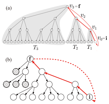
We apply Eq. (51) to the Brownian computation process schematically depicted as tree graphs (see Fig.10 of Ref. [5]). Figures 1 (a) and (b) show such graphs whose nodes represent logical states. In each panel, the bottom nodes are possible input states, and the top node corresponds to the output state. The computation proceeds from bottom to top, and the branching represents the logical irreversibility. In each panel, solid arcs constitute a directed rooted spanning tree . The computation starts from the start state, , which we take as the root, to the output state . There is an intended computation path with length , [thick solid arcs in panels (a) and (b)],
| (53) |
where . From each node on the intended computation path, a subtree rooted at the node grows [shaded parts in panel (a)]. The set of nodes is then , where . The nodes, except for the roots of the subtrees, represent extraneous predecessors; leaf nodes are either possible input states [bottom nodes in panels (a) and (b)] or ‘garden-of-Eden’ states with no predecessors [hatched nodes in panel (b)] [5]. All solid arcs are for bidirectional processes:
| (54) |
where .
The dotted arc in each panel is a chord representing the unidirectional reset process. The intended computation path and the reset path constitute a cycle:
| (55) |
The reset current is measured at the chord . We assume that there is no other chord, i.e., . Consequently, no free parameter exists in Eq. (51).
We focus on the signal-to-noise ratio (SNR) of the probability distribution of the computation time, which we define as the first passage time [4, 11], being upper bounded by TUR [19, 20, 32, 4]. The Fano factor of reset current and the SNR for resets are related as, [4].
From Eq. (51), the lower bound of the Fano factor is obtained as (Appendix D),
| (56) |
where is monotonically increasing in . The bound depends on the detailed structure of subtrees . In the following, we present analytic expressions for two examples.
The first example is the model of Brownian logically reversible Turing machine (RTM) [4, 11], in which extraneous predecessors are absent, and () for . Then, and thus the right-hand side of Eq. (56) becomes,
| (57) |
For , it approaches, as was obtained before [4].
The second example is the case where the directed rooted spanning tree forms a complete -ary tree () if we reverse arcs of the intended computation path [Fig. 1 (a)]. This case, the right-hand side of Eq. (56) becomes (Appendix E),
| (58) |
The lower bound approaches for . This behavior is reminiscent of the SNR observed for the token-based Brownian circuit [4]. The weaker bound, which follows from Eq. (56),
| (59) |
explains this behavior: The right-hand side approaches 1 when the extraneous predecessors are concentrating on the last subtree , . This condition is the case for the complete -ary tree-like graph, for .
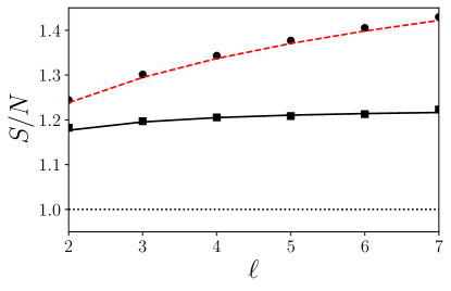
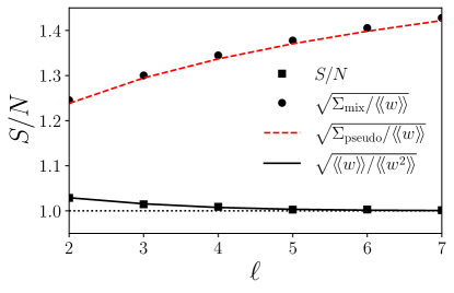
Figure 2 shows the SNR for a single reset () versus the length of the intended computation path . The top panel is for the Brownian RTM. The middle panel is for the complete 3-ary tree-like graph shown in Fig. 1 (a). In both panels, the analytic results, Eqs. (57) and (58) (solid lines) fit the numerical results (filled squares) obtained by the Gillespie algorithm. The SNR approaches in the top panel, while in the middle panel, the SNR quickly approaches 1, i.e., the logical irreversibility degrades the SNR.
In each panel, filled circles and the dashed line indicate the mixed and pseudo-entropy bounds, Eqs. (21) and (27),
| (60) | ||||
| (61) |
Here is the -th harmonic number, and is the Euler’s constant. Since the steady-state current only flows along the cycle, the entropy production depends only on the length of the intended computation path . It is independent of the number of the extraneous predecessors, which is large, e.g., there are extraneous states for the complete 3-ary tree-like graph with corresponding to the middle panel of Fig. 2. From this respect, the mixed and pseudo-entropy bounds are considered tight. However, they fail to capture the logical irreversibility and become logarithmically weaker for the longer intended computation path.
The bottom panel of Fig. 2 corresponds to the 3-ary tree-like graph, Fig. 1 (b). The SNR is bigger than one and smaller than mixed and pseudo-entropy bounds. Note that the average computation time itself, which is the reciprocal of the average reset current , increases with the number of extraneous states. We also note that the schematic Brownian computation models discussed here discard certain features of potential Brownian computation models: The token-based Brownian computation model [4] is concurrent and thus should contain many cycles in its graph. These cycles change the steady-state probabilities and alter the path-length dependence of mixed and pseudo-entropy bounds.

V Conclusion
Starting from the level 2.5 large deviation function, we derive a lower bound of the Fano factor expressed as a quadratic optimization problem in mesh currents subjected to a linear constraint. By the duality transformation and exploiting the root-to-node path matrix, we effectively integrate out fluctuations of sojourn times at all nodes when rates for bidirectional and unidirectional transitions are uniform. The bound applied to the schematic Brownian computation plus reset process shows that the logical irreversibility reduces the signal-to-noise ratio of the fluctuating computation time. It is contrasted with the mixed and pseudo-entropy bounds, which are independent of the logical irreversibility and become weaker logarithmically in the length of the intended computation path.
Acknowledgements.
We thank Satoshi Nakajima for proving the inequality (19). This work was supported by JSPS KAKENHI Grants No. 18KK0385, No. 20H01827, No. 20H05666, and No. 24K00547, and JST, CREST Grant Number JPMJCR20C1, Japan.Appendix A Proof of the inequality (19)
Let us introduce a function,
| (62) |
The first and second derivatives are,
| (63) | ||||
| (64) |
Since, for and for , is monotonically decreasing for and weakly increasing for . The zeros of are and ; Since and , there exists such that and . Then, for , and for and . Therefore, a local maximum and a local minimum exist at and , respectively. Since and the local minimum is , we conclude for , which proves (19).
Appendix B Proofs of Eqs. (33) and (34)
Equation (33) is calculated as, . If , it is 1 only when and 0 otherwise. If , it is (), when () is in the cycle . Therefore,
| (67) |
We introduce , the dual of , that maps to as, . By using this, the incidence matrix is expressed as . Then is calculated as,
| (68) |
if the cycle goes along the directions of twigs of , and
| (69) |
if goes in the direction opposite to . Here we write a path obtained from by removing as . For both equations, (68) and (69), we obtain , which proves Eq. (34).
Appendix C matrix
We write a unit vector as, , where and . Accordingly,
| (70) |
By substituting them into Eq. (43), we obtain,
| (71) |
Appendix D Derivations of Eq. (56)
By exploiting Eq. (16), the node state probability in the steady-state is,
| (72) |
The cycle matrix is . The nonzero components of matrix is for and for and (Appendix C). The mesh current satisfying the constraint is .
Appendix E Derivations of Eq. (58)
References
- Horowitz and Gingrich [2020] J. M. Horowitz and T. R. Gingrich, Thermodynamic uncertainty relations constrain non-equilibrium fluctuations, Nature Physics 16, 15 (2020).
- Shiraishi [2023] N. Shiraishi, An Introduction to Stochastic Thermodynamics: From Basic to Advanced (Springer Nature Singapore, Singapore, 2023).
- Wolpert [2020] D. H. Wolpert, Uncertainty relations and fluctuation theorems for bayes nets, Phys. Rev. Lett. 125, 200602 (2020).
- Utsumi et al. [2022] Y. Utsumi, Y. Ito, D. Golubev, and F. Peper, Computation time and thermodynamic uncertainty relation of brownian circuits, (2022), arXiv:2205.10735 [cond-mat.stat-mech] .
- Bennett [1982] C. H. Bennett, The thermodynamics of computation—a review, International Journal of Theoretical Physics 21, 905 (1982).
- Wolpert et al. [2023] D. Wolpert, J. Korbel, C. Lynn, F. Tasnim, J. Grochow, G. Kardeş, J. Aimone, V. Balasubramanian, E. de Giuli, D. Doty, N. Freitas, M. Marsili, T. E. Ouldridge, A. Richa, P. Riechers, Édgar Roldán, B. Rubenstein, Z. Toroczkai, and J. Paradiso, Is stochastic thermodynamics the key to understanding the energy costs of computation?, (2023), arXiv:2311.17166 [cond-mat.stat-mech] .
- Bryant [1961] P. Bryant, The algebra and topology of electrical networks, Proceedings of the IEE - Part C: Monographs 108, 215 (1961).
- Branin [1967] F. Branin, Computer methods of network analysis, Proceedings of the IEEE 55, 1787 (1967).
- Takahashi [1969] H. Takahashi, Theory of Linear Lumped Parameter System I, Kisokougaku, Iwanami kouza No. 6 (Iwanami shoten, Tokyo, 1969).
- Rasmussen et al. [2021] S. Rasmussen, K. Christensen, S. Pedersen, L. Kristensen, T. Bækkegaard, N. Loft, and N. Zinner, Superconducting circuit companion—an introduction with worked examples, PRX Quantum 2, 040204 (2021).
- Utsumi et al. [2023] Y. Utsumi, D. Golubev, and F. Peper, Thermodynamic cost of brownian computers in the stochastic thermodynamics of resetting, The European Physical Journal Special Topics 232, 3259 (2023).
- Bertini et al. [2015a] L. Bertini, A. Faggionato, and D. Gabrielli, Large deviations of the empirical flow for continuous time Markov chains, Annales de l’Institut Henri Poincaré, Probabilités et Statistiques 51, 867 (2015a).
- Bertini et al. [2015b] L. Bertini, A. Faggionato, and D. Gabrielli, Flows, currents, and cycles for markov chains: Large deviation asymptotics, Stochastic Processes and their Applications 125, 2786 (2015b).
- Barato and Chetrite [2015] A. C. Barato and R. Chetrite, A formal view on level 2.5 large deviations and fluctuation relations, Journal of Statistical Physics 160, 1154 (2015).
- Gingrich et al. [2016] T. R. Gingrich, J. M. Horowitz, N. Perunov, and J. L. England, Dissipation bounds all steady-state current fluctuations, Phys. Rev. Lett. 116, 120601 (2016).
- Pietzonka et al. [2016] P. Pietzonka, A. C. Barato, and U. Seifert, Affinity- and topology-dependent bound on current fluctuations, Journal of Physics A: Mathematical and Theoretical 49, 34LT01 (2016).
- Polettini et al. [2016] M. Polettini, A. Lazarescu, and M. Esposito, Tightening the uncertainty principle for stochastic currents, Phys. Rev. E 94, 052104 (2016).
- Gingrich et al. [2017] T. R. Gingrich, G. M. Rotskoff, and J. M. Horowitz, Inferring dissipation from current fluctuations, Journal of Physics A: Mathematical and Theoretical 50, 184004 (2017).
- Gingrich and Horowitz [2017] T. R. Gingrich and J. M. Horowitz, Fundamental bounds on first passage time fluctuations for currents, Phys. Rev. Lett. 119, 170601 (2017).
- Garrahan [2017] J. P. Garrahan, Simple bounds on fluctuations and uncertainty relations for first-passage times of counting observables, Phys. Rev. E 95, 032134 (2017).
- Andrieux and Gaspard [2007] D. Andrieux and P. Gaspard, Fluctuation theorem for currents and schnakenberg network theory, Journal of Statistical Physics 127, 107 (2007).
- Bagrets and Nazarov [2003] D. A. Bagrets and Y. V. Nazarov, Full counting statistics of charge transfer in coulomb blockade systems, Phys. Rev. B 67, 085316 (2003).
- Utsumi [2007] Y. Utsumi, Full counting statistics for the number of electrons in a quantum dot, Phys. Rev. B 75, 035333 (2007).
- Hill [1966] T. L. Hill, Studies in irreversible thermodynamics iv. diagrammatic representation of steady state fluxes for unimolecular systems, Journal of Theoretical Biology 10, 442 (1966).
- Schnakenberg [1976] J. Schnakenberg, Network theory of microscopic and macroscopic behavior of master equation systems, Re1978v. Mod. Phys. 48, 571 (1976).
- Weidlich [1978] W. Weidlich, On the structure of exact solutions of discrete masterequations, Zeitschrift für Physik B Condensed Matter 30, 345 (1978).
- Pal et al. [2021a] A. Pal, S. Reuveni, and S. Rahav, Thermodynamic uncertainty relation for systems with unidirectional transitions, Phys. Rev. Res. 3, 013273 (2021a).
- Shiraishi [2021] N. Shiraishi, Optimal thermodynamic uncertainty relation in markov jump processes, Journal of Statistical Physics 185, 19 (2021).
- Barato et al. [2018] A. C. Barato, R. Chetrite, A. Faggionato, and D. Gabrielli, Bounds on current fluctuations in periodically driven systems, New Journal of Physics 20, 103023 (2018).
- Gross and Kotiuga [2004] P. W. Gross and P. R. Kotiuga, Electromagnetic theory and computation: a topological approach, Mathematical Sciences Research Institute Publications, Vol. 48 (Cambridge University Press, Cambridge, 2004).
- Nagaosa [1999] N. Nagaosa, Problems related to superconductivity, in Quantum Field Theory in Condensed Matter Physics (Springer Berlin Heidelberg, Berlin, Heidelberg, 1999) pp. 113–160.
- Pal et al. [2021b] A. Pal, S. Reuveni, and S. Rahav, Thermodynamic uncertainty relation for first-passage times on markov chains, Phys. Rev. Res. 3, L032034 (2021b).