Strang Splitting for Parametric Inference in Second-order Stochastic Differential Equations

Abstract

We address parameter estimation in second-order stochastic differential equations (SDEs), prevalent in physics, biology, and ecology. Second-order SDE is converted to a first-order system by introducing an auxiliary velocity variable raising two main challenges. First, the system is hypoelliptic since the noise affects only the velocity, making the Euler-Maruyama estimator ill-conditioned. To overcome that, we propose an estimator based on the Strang splitting scheme. Second, since the velocity is rarely observed we adjust the estimator for partial observations. We present four estimators for complete and partial observations, using full likelihood or only velocity marginal likelihood. These estimators are intuitive, easy to implement, and computationally fast, and we prove their consistency and asymptotic normality. Our analysis demonstrates that using full likelihood with complete observations reduces the asymptotic variance of the diffusion estimator. With partial observations, the asymptotic variance increases due to information loss but remains unaffected by the likelihood choice. However, a numerical study on the Kramers oscillator reveals that using marginal likelihood for partial observations yields less biased estimators. We apply our approach to paleoclimate data from the Greenland ice core and fit it to the Kramers oscillator model, capturing transitions between metastable states reflecting observed climatic conditions during glacial eras.

Keywords Second-order stochastic differential equations, Hypoellipticity, Partial observations, Strang splitting estimator, Greenland ice core data, Kramers oscillator

1 Introduction

Second-order stochastic differential equations (SDEs) are an effective instrument for modeling complex systems showcasing both deterministic and stochastic dynamics, which incorporate the second derivative of a variable - the acceleration. These models are extensively applied in many fields, including physics (Rosenblum and Pikovsky, 2003), molecular dynamics (Leimkuhler and Matthews, 2015), ecology (Johnson et al., 2008; Michelot and Blackwell, 2019), paleoclimate research (Ditlevsen et al., 2002), and neuroscience (Ziv et al., 1994; Jansen and Rit, 1995).

The general form of a second-order SDE in Langevin form is given as follows:

$$\ddot{\mathbf{X}}_{t}=\mathbf{F}(\mathbf{X}_{t},\dot{\mathbf{X}}_{t},\bm{\beta})+\bm{\Sigma}\bm{\xi}_{t}.$$ (1)

Here, $\mathbf{X}_{t}\in\mathbb{R}^{d}$ denotes the variable of interest, the dot indicates derivative with respect to time $t$, drift $\mathbf{F}$ represents the deterministic force, and $\bm{\xi}_{t}$ is a white noise representing the system’s random perturbations around the deterministic force. We assume that $\bm{\Sigma}$ is constant, that is the noise is additive.

The main goal of this study is to estimate parameters in second-order SDEs. We first reformulate the $d$-dimensional second-order SDE (1) into a $2d$-dimensional SDE in Itô’s form. We define an auxiliary velocity variable, and express the second-order SDE in terms of its position $\mathbf{X}_{t}$ and velocity $\mathbf{V}_{t}$:

$$\operatorname*{\mathrm{d}\!}\mathbf{X}_{t} =\mathbf{V}_{t}\operatorname*{\mathrm{d}\!}t,\qquad \mathbf{X}_{0}=\mathbf{x}_{0},$$ (2)

$$\operatorname*{\mathrm{d}\!}\mathbf{V}_{t} =\mathbf{F}\left(\mathbf{X}_{t},\mathbf{V}_{t};\bm{\beta}\right)\operatorname*{\mathrm{d}\!}t+\bm{\Sigma}\operatorname*{\mathrm{d}\!}\mathbf{W}_{t},\qquad \mathbf{V}_{0}=\mathbf{v}_{0},$$

where $\mathbf{W}_{t}$ is a standard Wiener process. We refer to $\mathbf{X}_{t}$ and $\mathbf{V}_{t}$ as the smooth and rough coordinates, respectively.

A specific example of model (2) is $\mathbf{F}(\mathbf{x},\mathbf{v})=-\mathbf{c}(\mathbf{x},\mathbf{v})\mathbf{v}-\nabla\mathbf{U}(\mathbf{x})$, for some function $\mathbf{c}(\cdot)$ and potential $\mathbf{U}(\cdot)$. Then, model (2) is called a stochastic damping Hamiltonian system. This system describes the motion of a particle subjected to potential, dissipative, and random forces (Wu, 2001). An example of a stochastic damping Hamiltonian system is the Kramers oscillator introduced in Section 2.1.

Let $\mathbf{Y}_{t}=(\mathbf{X}_{t}^{\top},\mathbf{V}_{t}^{\top})^{\top}$, $\widetilde{\mathbf{F}}(\mathbf{x},\mathbf{v};\bm{\beta})=(\mathbf{v}^{\top},\mathbf{F}(\mathbf{x},\mathbf{v};\bm{\beta})^{\top})^{\top}$ and $\widetilde{\bm{\Sigma}}=(\mathbf{0}^{\top},\bm{\Sigma}^{\top})^{\top}$. Then (2) is formulated as

$$\operatorname*{\mathrm{d}\!}\mathbf{Y}_{t} =\widetilde{\mathbf{F}}\left(\mathbf{Y}_{t};\bm{\beta}\right)\operatorname*{\mathrm{d}\!}t+\widetilde{\bm{\Sigma}}\operatorname*{\mathrm{d}\!}\mathbf{W}_{t},\qquad\mathbf{Y}_{0}=\mathbf{y}_{0}.$$ (3)

The notation $\ \widetilde{}\$ over an object indicates that it is associated with process $\mathbf{Y}_{t}$. Specifically, the object is of dimension $2d$ or $2d\times 2d$.

When it exists, the unique solution of (3) is called a diffusion or diffusion process. System (3) is usually not fully observed since the velocity $\mathbf{V}_{t}$ is not observable. Thus, our primary objective is to estimate the underlying drift parameter $\bm{\beta}$ and the diffusion parameter ${\bm{\Sigma}}$, based on discrete observations of either $\mathbf{Y}_{t}$ (referred to as complete observation case), or only $\mathbf{X}_{t}$ (referred to as partial observation case). Diffusion $\mathbf{Y}_{t}$ is said to be hypoelliptic since the matrix

$$\widetilde{\bm{\Sigma}}\widetilde{\bm{\Sigma}}^{\top}=\begin{bmatrix}\bm{0}&\bm{0}\\ \bm{0}&\bm{\Sigma}\bm{\Sigma}^{\top}\end{bmatrix}$$ (4)

is not of full rank, while $\mathbf{Y}_{t}$ admits a smooth density. Thus, (2) is a subclass of a larger class of hypoelliptic diffusions.

Parametric estimation for hypoelliptic diffusions is an active area of research. Ditlevsen and Sørensen (2004) studied discretely observed integrated diffusion processes. They proposed to use prediction-based estimating functions, which are suitable for non-Markovian processes and which do not require access to the unobserved component. They proved consistency and asymptotic normality of the estimators for $N\to\infty$, but without any requirements on the sampling interval $h$. Certain moment conditions are needed to obtain results for fixed $h$, which are often difficult to fulfill for nonlinear drift functions. The estimator was applied to paleoclimate data in Ditlevsen et al. (2002), similar to the data we analyze in Section 5.

Gloter (2006) also focused on parametric estimation for discretely observed integrated diffusion processes, introducing a contrast function using the Euler-Maruyama discretization. He studied the asymptotic properties as the sampling interval $h\to 0$ and the sample size $N\to\infty$, under the so-called rapidly increasing experimental design $Nh\to\infty$ and $Nh^{2}\to 0$. To address the ill-conditioned contrast from the Euler-Maruyama discretization, he suggested using only the rough equations of the SDE. He proposed to recover the unobserved integrated component through the finite difference approximation $(\mathbf{X}_{t_{k+1}}-\mathbf{X}_{t_{k}})/h$. This approximation makes the estimator biased and requires a correction factor of 3/2 in one of the terms of the contrast function for partial observations. Consequently, the correction increases the asymptotic variance of the estimator of the diffusion parameter. Samson and Thieullen (2012) expanded the ideas of (Gloter, 2006) and proved the results of (Gloter, 2006) in more general models. Similar to (Gloter, 2006), their focus was on contrasts using the Euler-Maruyama discretization limited to only the rough equations.

Pokern et al. (2009) proposed an Itô-Taylor expansion, adding a noise term of order $h^{3/2}$ to the smooth component in the numerical scheme. They argued against the use of finite differences for approximating unobserved components. Instead, he suggested using the Itô-Taylor expansion leading to non-degenerate conditionally Gaussian approximations of the transition density and using Markov Chain Monte Carlo (MCMC) Gibbs samplers for conditionally imputing missing components based on the observations. They found out that this approach resulted in a biased estimator of the drift parameter of the rough component.

Ditlevsen and Samson (2019) focused on both filtering and inference methods for complete and partial observations. They proposed a contrast estimator based on the strong order 1.5 scheme (Kloeden and Platen, 1992), which incorporates noise of order $h^{3/2}$ into the smooth component, similar to (Pokern et al., 2009). Moreover, they retained terms of order $h^{2}$ in the mean, which removed the bias in the drift parameters noted in (Pokern et al., 2009). They proved consistency and asymptotic normality under complete observations, with the standard rapidly increasing experimental design $Nh\to\infty$ and $Nh^{2}\to 0$. They adopted an unconventional approach by using two separate contrast functions, resulting in marginal asymptotic results rather than a joint central limit theorem. The model was limited to a scalar smooth component and a diagonal diffusion coefficient matrix for the rough component.

Melnykova (2020) developed a contrast estimator using local linearization (LL) (Ozaki, 1985; Shoji and Ozaki, 1998; Ozaki et al., 2000) and compared it to the least-squares estimator. She employed local linearization of the drift function, providing a non-degenerate conditional Gaussian discretization scheme, enabling the construction of a contrast estimator that achieves asymptotic normality under the standard conditions $Nh\to\infty$ and $Nh^{2}\to 0$. She proved a joint central limit theorem, bypassing the need for two separate contrasts as in Ditlevsen and Samson (2019). The models in Ditlevsen and Samson (2019) and Melnykova (2020) allow for parameters in the smooth component of the drift, in contrast to models based on second-order differential equations.

Recent work by Gloter and Yoshida (2020, 2021) introduced adaptive and non-adaptive methods in hypoelliptic diffusion models, proving asymptotic normality in the complete observation regime. In line with this work, we briefly review their non-adaptive estimator. It is based on a higher-order Itô-Taylor expansion that introduces additional Gaussian noise onto the smooth coordinates, accompanied by an appropriate higher-order mean approximation of the rough coordinates. The resulting estimator was later termed the local Gaussian (LG), which should be differentiated from LL. The LG estimator can be viewed as an extension of the estimator proposed in Ditlevsen and Samson (2019), with fewer restrictions on the class of models. Gloter and Yoshida (2020, 2021) found that using the full SDE to create a contrast reduces the asymptotic variance of the estimator of the diffusion parameter compared to methods using only rough coordinates in the case of complete observations.

The most recent contributions are Iguchi et al. (2023a, b); Iguchi and Beskos (2023), building on the foundation of the LG estimator and focusing on high-frequency regimes addressing limitations in earlier methods. Iguchi et al. (2023b) presented a new closed-form contrast estimator for hypoelliptic SDEs (denoted as Hypo-I) based on Edgeworth-type density expansion and Malliavin calculus that achieves asymptotic normality under the less restrictive condition of $Nh^{3}\to 0$. Iguchi et al. (2023a) focused on a highly degenerate class of SDEs (denoted as Hypo-II) where smooth coordinates split into further sub-groups and proposed estimators for both complete and partial observation settings. Iguchi and Beskos (2023) further refined the conditions for estimators asymptotic normality for both Hypo-I and Hypo-II under a weak design $Nh^{p}\to 0$, for $p\geq 2$.

The existing methods are generally based on approximations with varying degrees of refinements to correct for possible nonlinearities. This implies that they quickly degrade for highly nonlinear models if the step size is increased. In particular, this is the case for Hamiltonian systems. Instead, we propose to use splitting schemes, more precisely the Strang splitting scheme.

Splitting schemes are established techniques initially developed for solving ordinary differential equations (ODEs) and have proven to be effective also for SDEs (Ableidinger et al., 2017; Buckwar et al., 2022; Pilipovic et al., 2024). These schemes yield accurate results in many practical applications since they incorporate nonlinearities in their construction. This makes them particularly suitable for second-order SDEs, where they have been widely used. Early work in dissipative particle dynamics (Shardlow, 2003; Serrano et al., 2006), applications to molecular dynamics (Vanden-Eijnden and Ciccotti, 2006; Melchionna, 2007; Leimkuhler and Matthews, 2015) and studies on internal particles (Pavliotis et al., 2009) all highlight the scheme’s versatility. Burrage et al. (2007), Bou-Rabee and Owhadi (2010), and Abdulle et al. (2015) focused on the long-run statistical properties such as invariant measures. Bou-Rabee (2017); Bréhier and Goudenège (2019) and Adams et al. (2022) used splitting schemes for stochastic partial differential equations (SPDEs).

Despite the extensive use of splitting schemes in different areas, statistical applications have been lacking. We have recently proposed statistical estimators for elliptic SDEs (Pilipovic et al., 2024). The straightforward and intuitive schemes lead to robust, easy-to-implement estimators, offering an advantage over more numerically intensive and less user-friendly state-of-the-art methods. We use the Strang splitting scheme to approximate the transition density between two consecutive observations and derive the pseudo-likelihood function since the exact likelihood function is often unknown or intractable. Then, to estimate parameters, we employ maximum likelihood estimation (MLE). However, two specific statistical problems arise due to hypoellipticity and partial observations.

First, hypoellipticity leads to degenerate Euler-Maruyama transition schemes, which can be addressed by constructing the pseudo-likelihood solely from the rough equations of the SDE, referred to as the rough likelihood hereafter. The Strang splitting technique enables the estimator to incorporate both smooth and rough components (referred to as the full likelihood). It is also possible to construct Strang splitting estimators using only the rough likelihood, raising the question of which estimator performs better. Our results are in line with Gloter and Yoshida (2020, 2021) in the complete observation setting, where we find that using the full likelihood reduces the asymptotic variance of the diffusion estimator. We found the same results in the simulation study for the LL estimator proposed by Melnykova (2020).

Second, we suggest to treat the unobserved velocity by approximating it using finite difference methods. While Gloter (2006) and Samson and Thieullen (2012) exclusively use forward differences, we investigate also central and backward differences. The forward difference approach leads to a biased estimator unless it is corrected. One of the main contributions of this work is finding suitable corrections of the pseudo-likelihoods for different finite difference approximations such that the Strang estimators are asymptotically unbiased. This also ensures consistency of the diffusion parameter estimator, at the cost of increasing its asymptotic variance.

When only partial observations are available, we explore the impact of using the full likelihood versus the rough likelihood and how different finite differentiation approximations influence the parametric inference. We find that the choice of likelihood does not affect the asymptotic variance of the estimator. However, our simulation study on the Kramers oscillator suggests that using the full likelihood in finite sample setups introduce more bias than using only the rough marginal likelihood, which is the opposite of the complete observation setting. Finally, we analyze a paleoclimate ice core dataset from Greenland using a second-order SDE.

The main contributions of this paper are:

1. We extend the Strang splitting estimator of (Pilipovic et al., 2024) to hypoelliptic models given by second-order SDEs, including appropriate correction factors to obtain consistency.

2. When complete observations are available, we show that the asymptotic variance of the estimator of the diffusion parameter is smaller when maximizing the full likelihood. In contrast, for partial observations, we show that the asymptotic variance remains unchanged regardless of using the full or marginal likelihood of the rough coordinates.

3. We discuss the influence on the statistical properties of using the forward difference approximation for imputing the unobserved velocity variables compared to using the backward or the central difference.

4. We evaluate the performance of the estimators through a simulation study of a second-order SDE, the Kramers oscillator. Additionally, we show numerically in a finite sample study that the marginal likelihood for partial observations is more favorable than the full likelihood.

5. We fit the Kramers oscillator to a paleoclimate ice core dataset from Greenland and estimate the average time needed to pass between two metastable states.

The structure of the paper is as follows. In Section 2, we introduce the class of SDE models, define hypoellipticity, introduce the Kramers oscillator, and explain the Strang splitting scheme and its associated estimators. The asymptotic properties of the estimator are established in Section 3. The theoretical results are illustrated in a simulation study on the Kramers Oscillator in Section 4. Section 5 illustrates our methodology on the Greenland ice core data, while the technical results and the proofs of the main theorems and properties are in Section 6 and Supplementary Material S1, respectively.

Notation. We use capital bold letters for random vectors, vector-valued functions, and matrices, while lowercase bold letters denote deterministic vectors. $\|\cdot\|$ denotes both the $L^{2}$ vector norm in $\mathbb{R}^{d}$. Superscript $(i)$ on a vector denotes the $i$-th component, while on a matrix it denotes the $i$-th column. Double subscript $ij$ on a matrix denotes the component in the $i$-th row and $j$-th column. The transpose is denoted by $\top$. Operator $\operatorname*{Tr}(\cdot)$ returns the trace of a matrix and $\det(\cdot)$ the determinant. $\mathbf{I}_{d}$ denotes the $d$-dimensional identity matrix, while $\bm{0}_{d\times d}$ is a $d$-dimensional zero square matrix. We denote by $[a_{i}]_{i=1}^{d}$ a vector with coordinates $a_{i}$, and by $[b_{ij}]_{i,j=1}^{d}$ a matrix with coordinates $b_{ij}$, for $i,j=1,\ldots,d$. For a real-valued function $g:\mathbb{R}^{d}\to\mathbb{R}$, $\partial_{x^{(i)}}g(\mathbf{x})$ denotes the partial derivative with respect to $x^{(i)}$ and $\partial_{x^{(i)}x^{(j)}}^{2}g(\mathbf{x})$ denotes the second partial derivative with respect to $x^{(i)}$ and $x^{(j)}$. The nabla operator $\nabla_{\mathbf{x}}$ denotes the gradient vector of $g$ with respect of $\mathbf{x}$, that is, $\nabla_{\mathbf{x}}g(\mathbf{x})=[\partial_{x^{(i)}}g(\mathbf{x})]_{i=1}^{d}$. $\mathbb{H}$ denotes the Hessian matrix of function $g$, $\mathbb{H}_{g}(\mathbf{x})=[\partial_{x^{(i)}x^{(j)}}g(\mathbf{x})]_{i,j=1}^{d}$. For a vector-valued function $\mathbf{F}:\mathbb{R}^{d}\to\mathbb{R}^{d}$, the differential operator $D_{\mathbf{x}}$ denotes the Jacobian matrix $D_{\mathbf{x}}\mathbf{F}(\mathbf{x})=[\partial_{x^{(i)}}F^{(j)}(\mathbf{x})]_{i,j=1}^{d}$. Let $\mathbf{R}$ represent a vector (or a matrix) valued function defined on $(0,1)\times\mathbb{R}^{d}$ (or $(0,1)\times\mathbb{R}^{d\times d}$), such that, for some constant $C$, $\|\mathbf{R}(a,\mathbf{x})\|<aC(1+\|\mathbf{x}\|)^{C}$ for all $a,\mathbf{x}$. When denoted by $R$, it refers to a scalar function. For an open set $A$, the bar $\overline{A}$ indicates closure. We write $\xrightarrow{\mathbb{P}}$ for convergence in probability $\mathbb{P}$.

2 Problem setup

Let $\mathbf{Y}=(\mathbf{Y}_{t})_{t\geq 0}$ in (3) be defined on a complete probability space $(\Omega,\mathcal{F},\mathbb{P}_{\bm{\theta}})$ with a complete right-continuous filtration $\mathcal{F}=(\mathcal{F}_{t})_{t\geq 0}$, and let the $d$-dimensional Wiener process $\mathbf{W}=(\mathbf{W}_{t})_{t\geq 0}$ be adapted to $\mathcal{F}_{t}$. The probability measure $\mathbb{P}_{\bm{\theta}}$ is parameterized by the parameter $\bm{\theta}=\left(\bm{\beta},\bm{\Sigma}\right)$. Rewrite equation (3) as follows:

$$\operatorname*{\mathrm{d}\!}\mathbf{Y}_{t}=\widetilde{\mathbf{A}}(\bm{\beta})(\mathbf{Y}_{t}-\widetilde{\mathbf{b}}(\bm{\beta}))\operatorname*{\mathrm{d}\!}t+\widetilde{\mathbf{N}}\left(\mathbf{Y}_{t};\bm{\beta}\right)\operatorname*{\mathrm{d}\!}t+\widetilde{\bm{\Sigma}}\operatorname*{\mathrm{d}\!}\mathbf{W}_{t},$$ (5)

where

$$\widetilde{\mathbf{A}}(\bm{\beta})=\begin{bmatrix}\bm{0}_{d\times d}&\mathbf{I}_{d}\\ \mathbf{A}_{\mathbf{x}}(\bm{\beta})&\mathbf{A}_{\mathbf{v}}(\bm{\beta})\end{bmatrix},\quad\widetilde{\mathbf{b}}(\bm{\beta})=\begin{bmatrix}\mathbf{b}(\bm{\beta})\\ \bm{0}_{d}\end{bmatrix},\quad\widetilde{\mathbf{N}}(\mathbf{x},\mathbf{v};\bm{\beta})=\begin{bmatrix}\bm{0}_{d}\\ \mathbf{N}(\mathbf{x},\mathbf{v};\bm{\beta})\end{bmatrix}.$$ (6)

Function $\mathbf{F}$ in (2) is thus split as $\mathbf{F}(\mathbf{x},\mathbf{v};\bm{\beta})=\mathbf{A}_{\mathbf{x}}(\bm{\beta})(\mathbf{x}-\mathbf{b}(\bm{\beta}))+\mathbf{A}_{\mathbf{v}}(\bm{\beta})\mathbf{v}+\mathbf{N}(\mathbf{x},\mathbf{v};\bm{\beta})$.

Let $\overline{\Theta}_{\beta}\times\overline{\Theta}_{\Sigma}=\overline{\Theta}$ denote the closure of the parameter space with $\Theta_{\beta}$ and $\Theta_{\Sigma}$ being two convex open bounded subsets of $\mathbb{R}^{r}$ and $\mathbb{R}^{d\times d}$, respectively. The function $\mathbf{N}:\mathbb{R}^{2d}\times\overline{\Theta}_{\beta}\to\mathbb{R}^{d}$ is assumed locally Lipschitz; functions $\mathbf{A}_{\mathbf{x}}$ and $\mathbf{A}_{\mathbf{v}}$ are defined on $\overline{\Theta}_{\beta}$ and take values in $\mathbb{R}^{d\times d}$; and the parameter matrix $\bm{\Sigma}$ takes values in $\mathbb{R}^{d\times d}$. The matrix $\bm{\Sigma}\bm{\Sigma}^{\top}$ is assumed to be positive definite, shaping the variance of the rough coordinates. As any square root of $\bm{\Sigma}\bm{\Sigma}^{\top}$ induces the same distribution, $\bm{\Sigma}$ is identifiable only up to equivalence classes. Hence, estimation of the parameter $\bm{\Sigma}$ means estimation of $\bm{\Sigma}\bm{\Sigma}^{\top}$. The drift function $\widetilde{\mathbf{F}}$ in (3) is divided into a linear part given by the matrix $\widetilde{\mathbf{A}}$ and a nonlinear part given by $\widetilde{\mathbf{N}}$.

The true value of the parameter is denoted by $\bm{\theta}_{0}=\left(\bm{\beta}_{0},\bm{\Sigma}_{0}\right)$, and we assume that $\bm{\theta}_{0}\in\Theta$. When referring to the true parameters, we write $\mathbf{A}_{\mathbf{x},0}$, $\mathbf{A}_{\mathbf{v},0}$, $\mathbf{b}_{0}$, $\mathbf{N}_{0}(\mathbf{x})$, $\mathbf{F}_{0}(\mathbf{x})$ and $\bm{\Sigma}\bm{\Sigma}_{0}^{\top}$ instead of $\mathbf{A}_{\mathbf{x}}(\bm{\beta}_{0})$, $\mathbf{A}_{\mathbf{v}}(\bm{\beta}_{0})$, $\mathbf{b}(\bm{\beta}_{0})$, $\mathbf{N}(\mathbf{x};\bm{\beta}_{0})$, $\mathbf{F}(\mathbf{x};\bm{\beta}_{0})$ and $\bm{\Sigma}_{0}\bm{\Sigma}_{0}^{\top}$, respectively. We write $\mathbf{A}_{\mathbf{x}}$, $\mathbf{A}_{\mathbf{v}}$, $\mathbf{b}$, $\mathbf{N}(\mathbf{x})$, $\mathbf{F}(\mathbf{x})$, and $\bm{\Sigma}\bm{\Sigma}^{\top}$ for any parameter $\bm{\theta}$.

2.1 Example: The Kramers oscillator

The abrupt temperature changes during the ice ages, known as the Dansgaard–Oeschger (DO) events, are essential elements for understanding the climate (Dansgaard et al., 1993). These events occurred during the last glacial era spanning approximately the period from 115,000 to 12,000 years before present and are characterized by rapid warming phases followed by gradual cooling periods, revealing colder (stadial) and warmer (interstadial) climate states (Rasmussen et al., 2014).

To analyze the DO events in Section 5, we propose a stochastic model of the escape dynamics in metastable systems, the Kramers oscillator (Kramers, 1940), originally formulated to model the escape rate of Brownian particles from potential wells. The escape rate is related to the mean first passage time — the time needed for a particle to exceed the potential’s local maximum for the first time, starting at a neighboring local minimum. This rate depends on variables such as the damping coefficient, noise intensity, temperature, and specific potential features, including the barrier’s height and curvature at the minima and maxima. We apply this framework to quantify the rate of climate transitions between stadial and interstadial periods. This provides an estimate on the probability distribution of the ocurrence of DO events, contributing to our understanding of the global climate system.

Following Arnold and Imkeller (2000), we introduce the Kramers oscillator as the stochastic Duffing oscillator - an example of a second-order SDE and a stochastic damping Hamiltonian system. The Duffing oscillator (Duffing, 1918) is a forced nonlinear oscillator, featuring a cubic stiffness term. The governing equation is given by:

$$\ddot{x}_{t}+\eta\dot{x}_{t}+\frac{\operatorname*{\mathrm{d}\!}}{\operatorname*{\mathrm{d}\!}x}U(x_{t})=f(t),\quad\text{where}\quad U(x)=-a\frac{x^{2}}{2}+b\frac{x^{4}}{4},\quad\text{with}\quad a,b>0,\quad\eta\geq 0.$$ (7)

The parameter $\eta$ in (7) indicates the damping level, $a$ regulates the linear stiffness, and $b$ determines the nonlinear component of the restoring force. In the special case where $b=0$, the equation simplifies to a damped harmonic oscillator. Function $f$ represents the driving force and is usually set to $f(t)=\eta\cos(\omega t)$, which introduces deterministic chaos (Korsch and Jodl, 1999).

When the driving force is $f(t)=\sqrt{2\eta\mathrm{T}}\xi(t)$, where $\xi(t)$ is white noise, equation (7) characterizes the stochastic movement of a particle within a bistable potential well, interpreting $\mathrm{T}>0$ as the temperature of a heat bath. Setting $\sigma=\sqrt{2\eta\mathrm{T}}$, equation (7) can be reformulated as an Itô SDE for variables $X_{t}$ and $V_{t}=\dot{X}_{t}$, expressed as:

$$\operatorname*{\mathrm{d}\!}X_{t} =V_{t}\operatorname*{\mathrm{d}\!}t,$$ (8)

$$\operatorname*{\mathrm{d}\!}V_{t} =\left(-\eta V_{t}-\frac{\operatorname*{\mathrm{d}\!}}{\operatorname*{\mathrm{d}\!}x}U(X_{t})\right)\operatorname*{\mathrm{d}\!}t+\sigma\operatorname*{\mathrm{d}\!}W_{t},$$

where $W_{t}$ denotes a standard Wiener process. The parameter set of SDE (8) is $\bm{\theta}=\{\eta,a,b,\sigma^{2}\}$.

The existence and uniqueness of the invariant measure $\nu_{0}(\operatorname*{\mathrm{d}\!}x,\operatorname*{\mathrm{d}\!}y)$ of (8) is proved in Theorem 3 in (Arnold and Imkeller, 2000). The invariant measure $\nu_{0}$ is linked to the invariant density $\pi_{0}$ through $\nu_{0}(\operatorname*{\mathrm{d}\!}x,\operatorname*{\mathrm{d}\!}y)=\pi_{0}(x,v)\operatorname*{\mathrm{d}\!}x\operatorname*{\mathrm{d}\!}y$. Here we write $\pi_{0}(x,v)$ instead of $\pi(x,v;\bm{\theta}_{0})$, and $\pi(x,v)$ instead of $\pi(x,v;\bm{\theta})$. The Fokker-Plank equation for $\pi$ is given by

$$-v\frac{\partial}{\partial x}\pi(x,v)+\eta\pi(x,v)+\eta v\frac{\partial}{\partial v}\pi(x,v)+\frac{\operatorname*{\mathrm{d}\!}}{\operatorname*{\mathrm{d}\!}x}U(x)\frac{\partial}{\partial v}\pi(x,v)+\frac{\sigma^{2}}{2}\frac{\partial^{2}}{\partial v^{2}}\pi(x,v)=0.$$ (9)

The invariant density that solves the Fokker-Plank equation is:

$$\pi(x,v)=C\exp\left(-\frac{2\eta}{\sigma^{2}}U(x)\right)\exp\left(-\frac{\eta}{\sigma^{2}}v^{2}\right),$$ (10)

where $C$ is the normalizing constant.

The marginal invariant probability of $V_{t}$ is thus Gaussian with zero mean and variance $\sigma^{2}/(2\eta)$. The marginal invariant probability of $X_{t}$ is bimodal driven by the potential $U(x)$:

$$\pi(x)=C\exp\left(-\frac{2\eta}{\sigma^{2}}U(x)\right).$$ (11)

At steady state, for a particle moving in any potential $U(x)$ and driven by random Gaussian noise, the position $x$ and velocity $v$ are independent of each other. This is reflected by the decomposition of the joint density $\pi(x,v)$ into $\pi(x)\pi(v)$.

Fokker-Plank equation (9) can also be used to derive the mean first passage time $\tau$ which is inversely related to Kramers’ escape rate $\kappa$ (Kramers, 1940):

$$\tau=\frac{1}{\kappa}\approx\frac{2\pi}{\left(\sqrt{1+\frac{\eta^{2}}{4\omega^{2}}}-\frac{\eta}{2\omega}\right)\Omega}\exp\left(\frac{\Delta U}{\rm T}\right),$$

where $x_{\mathrm{barrier}}=0$ is the local maximum of $U(x)$ and $x_{\mathrm{well}}=\pm\sqrt{a/b}$ are the local minima, $\omega=\sqrt{|U^{\prime\prime}(x_{\mathrm{barrier}})|}=\sqrt{a}$, $\Omega=\sqrt{U^{\prime\prime}(x_{\mathrm{well}})}=\sqrt{2a}$, and $\Delta U=U(x_{\mathrm{barrier}})-U(x_{\mathrm{well}})=a^{2}/4b$, . The formula is derived assuming strong friction, or an over-damped system ($\eta\gg\omega$), and a small parameter $\mathrm{T}/\Delta U\ll 1$, indicating sufficiently deep potential wells. For the potential defined in (7), the mean waiting time $\tau$ is then approximated by

$$\tau\approx\frac{\sqrt{2}\pi}{\sqrt{a+\frac{\eta^{2}}{4}}-\frac{\eta}{2}}\exp\left(\frac{a^{2}\eta}{2b\sigma^{2}}\right).$$ (12)

2.2 Hypoellipticity

The SDE (5) is said to be hypoelliptic if its quadratic diffusion matrix $\widetilde{\bm{\Sigma}}\widetilde{\bm{\Sigma}}^{\top}$ is not of full rank, while its solutions admit a smooth transition density with respect to the Lebesgue measure. According to Hörmander’s theorem (Nualart, 2006), this is fulfilled if the SDE in its Stratonovich form satisfies the weak Hörmander condition. Since $\bm{\Sigma}$ does not depend on $\mathbf{y}$, the Itô and Stratonovich forms coincide.

We begin by recalling the concept of Lie brackets: for smooth vector fields $\bm{f},\bm{g}:\mathbb{R}^{2d}\to\mathbb{R}^{2d}$, the $i$-th component of the Lie bracket, $[\bm{f},\bm{g}]^{(i)}$, is defined as

$$[\bm{f},\bm{g}]^{(i)}\coloneqq D_{\mathbf{y}}^{\top}g^{(i)}(\mathbf{y})\bm{f}(\mathbf{y})-D_{\mathbf{y}}^{\top}f^{(i)}(\mathbf{y})\bm{g}(\mathbf{y}).$$

We define the set $\mathcal{H}$ of vector fields by initially including $\widetilde{\bm{\Sigma}}^{(i)}$, $i=1,2,...,2d$, and then recursively adding Lie brackets

$$H\in\mathcal{H}\Rightarrow[\widetilde{\mathbf{F}},H],[\widetilde{\bm{\Sigma}}^{(1)},H],\dots,[\widetilde{\bm{\Sigma}}^{(2d)},H]\in\mathcal{H}.$$

The weak Hörmander condition is met if the vectors in $\mathcal{H}$ span $\mathbb{R}^{2d}$ at every point $\mathbf{y}\in\mathbb{R}^{2d}$. The initial vectors span $\{(\mathbf{0},\mathbf{v})\in\mathbb{R}^{2d}\mid\mathbf{v}\in\mathbb{R}^{d}\}$, a $d$-dimensional subspace. We therefore need to verify the existence of some $H\in\mathcal{H}$ with a non-zero first element. The first iteration of the system yields

$$[\widetilde{\mathbf{F}},\widetilde{\bm{\Sigma}}^{(i)}]^{(1)} =-\bm{\Sigma}^{(i)},$$

$$[\widetilde{\bm{\Sigma}}^{(i)},\widetilde{\bm{\Sigma}}^{(j)}]^{(1)} =\mathbf{0},$$

for $i,j=1,2,...,2d$. The first equation is non-zero, as are all subsequent iterations. Thus, the second-order SDE defined in (5) is always hypoelliptic.

2.3 Assumptions

The following assumptions are a generalization of those presented in (Pilipovic et al., 2024).

Let $T>0$ be the length of the observed time interval. We assume that (5) has a unique strong solution $\mathbf{Y}=\{\mathbf{Y}_{t}\mid t\in[0,T]\}$, adapted to $\mathcal{F}=\{\mathcal{F}_{t}\mid t\in[0,T]\}$, which follows from the following first two assumptions (Theorem 2 in Alyushina (1988), Theorem 1 in Krylov (1991), Theorem 3.5 in Mao (2007)). We need the last three assumptions to prove the properties of the estimators.

• Function ${\mathbf{N}}$ is twice continuously differentiable with respect to both $\mathbf{y}$ and $\bm{\theta}$, i.e., ${\mathbf{N}}\in C^{2}$. Moreover, it is globally one-sided Lipschitz continuous with respect to $\mathbf{y}$ on $\mathbb{R}^{2d}\times\overline{\Theta}_{\beta}$. That is, there exists a constant $C>0$ such that for all $\mathbf{y}_{1},\mathbf{y}_{2}\in\mathbb{R}^{2d}$,

  $$\left(\mathbf{y}_{1}-\mathbf{y}_{2}\right)^{\top}\left({\mathbf{N}}(\mathbf{y}_{1};\bm{\beta})-{\mathbf{N}}(\mathbf{y}_{2};\bm{\beta})\right)\leq C\|\mathbf{y}_{1}-\mathbf{y}_{2}\|^{2}.$$

• Function ${\mathbf{N}}$ exhibits at most polynomial growth in $\mathbf{y}$, uniformly in $\bm{\theta}$. Specifically, there exist constants $C>0$ and $\chi\geq 1$ such that for all $\mathbf{y}_{1},\mathbf{y}_{2}\in\mathbb{R}^{2d}$,

  $$\|{\mathbf{N}}\left(\mathbf{y}_{1};\bm{\beta}\right)-{\mathbf{N}}\left(\mathbf{y}_{2};\bm{\beta}\right)\|^{2}\leq C\left(1+\|\mathbf{y}_{1}\|^{2\chi-2}+\|\mathbf{y}_{2}\|^{2\chi-2}\right)\|\mathbf{y}_{1}-\mathbf{y}_{2}\|^{2}.$$

  Additionally, its derivatives exhibit polynomial growth in $\mathbf{y}$, uniformly in $\bm{\theta}$.

• The solution $\mathbf{Y}$ to SDE (5) has invariant probability $\nu_{0}(\operatorname*{\mathrm{d}\!}\mathbf{y})$.

• $\bm{\Sigma}\bm{\Sigma}^{\top}$ is invertible on $\overline{\Theta}_{\Sigma}$.

• $\bm{\beta}$ is identifiable, that is, if $\mathbf{F}(\mathbf{y},\bm{\beta}_{1})=\mathbf{F}(\mathbf{y},\bm{\beta}_{2})$ for all $\mathbf{y}\in\mathbb{R}^{2d}$, then $\bm{\beta}_{1}=\bm{\beta}_{2}$.

Assumption (A1) ensures finiteness of the moments of the solution $\mathbf{X}$ (Tretyakov and Zhang, 2013), i.e.,

$$\mathbb{E}[\sup\limits_{t\in[0,T]}\|\mathbf{Y}_{t}\|^{{2p}}]<C(1+\|\mathbf{y}_{0}\|^{{2p}}),\hskip 12.91663pt\forall{\,p\geq 1}.$$ (13)

Assumption (A3) is necessary for the ergodic theorem to ensure convergence in distribution. Assumption (A4) ensures that the model (5) is hypoelliptic. Assumption (A5) ensures the identifiability of the drift parameter.

2.4 Strang splitting scheme

Consider the following splitting of (5):

$$\operatorname*{\mathrm{d}\!}\mathbf{Y}^{[1]}_{t} =\widetilde{\mathbf{A}}(\mathbf{Y}^{[1]}_{t}-\widetilde{\mathbf{b}})\operatorname*{\mathrm{d}\!}t+\widetilde{\bm{\Sigma}}\operatorname*{\mathrm{d}\!}\mathbf{W}_{t}, \mathbf{Y}^{[1]}_{0}=\mathbf{y}_{0},$$ (14)

$$\operatorname*{\mathrm{d}\!}\mathbf{Y}^{[2]}_{t} =\widetilde{\mathbf{N}}(\mathbf{Y}^{[2]}_{t})\operatorname*{\mathrm{d}\!}t, \mathbf{Y}^{[2]}_{0}=\mathbf{y}_{0}.$$ (15)

There are no assumptions on the choice of $\widetilde{\mathbf{A}}$ and $\widetilde{\mathbf{b}}$, and thus the nonlinear function $\widetilde{\mathbf{N}}$. Indeed, we show that the asymptotic results hold for any choice of $\widetilde{\mathbf{A}}$ and $\widetilde{\mathbf{b}}$ in both the complete and the partial observation settings. This extends the results in Pilipovic et al. (2024), where it is shown to hold in the elliptic complete observation case, as well. While asymptotic results are invariant to the choice of $\widetilde{\mathbf{A}}$ and $\widetilde{\mathbf{b}}$, finite sample properties of the scheme and the corresponding estimators are very different, and it is important to choose the splitting wisely. Intuitively, when the process is close to a fixed point of the drift, the linear dynamics are dominating, whereas far from the fixed points, the nonlinearities might be dominating. If the drift has a fixed point $\mathbf{y}^{\star}$, we therefore suggest setting $\widetilde{\mathbf{A}}=D_{\mathbf{y}}\widetilde{\mathbf{F}}(\mathbf{y}^{\star})$ and $\widetilde{\mathbf{b}}=\mathbf{y}^{\star}$. This choice is confirmed in simulations (for more details see Pilipovic et al. (2024)).

Solution of SDE (14) is an Ornstein–Uhlenbeck (OU) process given by the following $h$-flow:

$$\mathbf{Y}_{t_{k}}^{[1]} =\Phi_{h}^{[1]}(\mathbf{Y}_{t_{k-1}}^{[1]})=\widetilde{\bm{\mu}}_{h}(\mathbf{Y}_{t_{k-1}}^{[1]};\bm{\beta})+\widetilde{\bm{\varepsilon}}_{h,k},$$ (16)

$$\widetilde{\bm{\mu}}_{h}(\mathbf{y};\bm{\beta}) \coloneqq e^{\widetilde{\mathbf{A}}h}(\mathbf{y}-\widetilde{\mathbf{b}})+\widetilde{\mathbf{b}},$$ (17)

$$\widetilde{\bm{\Omega}}_{h} =\int_{0}^{h}e^{\widetilde{\mathbf{A}}(h-u)}\widetilde{\bm{\Sigma}}\widetilde{\bm{\Sigma}}^{\top}e^{\widetilde{\mathbf{A}}^{\top}(h-u)}\operatorname*{\mathrm{d}\!}u,$$ (18)

where $\widetilde{\bm{\varepsilon}}_{h,k}\stackrel{{\scriptstyle i.i.d}}{{\sim}}\mathcal{N}_{2d}(\bm{0},\widetilde{\bm{\Omega}}_{h})$ for $k=1,\ldots,N$. It is useful to rewrite $\widetilde{\bm{\Omega}}_{h}$ in the following block matrix form,

$$\widetilde{\bm{\Omega}}_{h}=\begin{bmatrix}\bm{\Omega}_{h}^{\mathrm{[SS]}}&\bm{\Omega}_{h}^{\mathrm{[SR]}}\\ \bm{\Omega}_{h}^{\mathrm{[RS]}}&\bm{\Omega}_{h}^{\mathrm{[RR]}}\end{bmatrix},$$ (19)

where $\mathrm{S}$ in the superscript stands for smooth and $\mathrm{R}$ stands for rough. The Schur complement of $\widetilde{\bm{\Omega}}_{h}$ with respect to $\bm{\Omega}_{h}^{\mathrm{[RR]}}$ and the determinant of $\widetilde{\bm{\Omega}}_{h}$ are given by:

$$\bm{\Omega}_{h}^{\mathrm{[S|R]}}\coloneqq\bm{\Omega}_{h}^{\mathrm{[SS]}}-\bm{\Omega}_{h}^{\mathrm{[SR]}}(\bm{\Omega}_{h}^{\mathrm{[RR]}})^{-1}\bm{\Omega}_{h}^{\mathrm{[RS]}},\qquad\det\widetilde{\bm{\Omega}}_{h}=\det\bm{\Omega}_{h}^{\mathrm{[RR]}}\det\bm{\Omega}_{h}^{\mathrm{[S\mid R]}}.$$

Assumptions (A1)-(A2) ensure the existence and uniqueness of the solution of (15) (Theorem 1.2.17 in Humphries and Stuart (2002)). Thus, there exists a unique function $\widetilde{\bm{f}}_{h}:\mathbb{R}^{2d}\times\Theta_{\beta}\to\mathbb{R}^{2d}$, for $h\geq 0$, such that

$$\mathbf{Y}_{t_{k}}^{[2]}=\Phi_{h}^{[2]}(\mathbf{Y}_{t_{k-1}}^{[2]})=\widetilde{\bm{f}}_{h}(\mathbf{Y}_{t_{k-1}}^{[2]};\bm{\beta}).$$ (20)

For all $\bm{\beta}\in\Theta_{\beta}$, the $h$-flow $\widetilde{\bm{f}}_{h}$ fulfills the following semi-group properties:

$$\widetilde{\bm{f}}_{0}(\mathbf{y};\bm{\beta}) =\mathbf{y},\qquad\widetilde{\bm{f}}_{t+s}(\mathbf{y};\bm{\beta})=\widetilde{\bm{f}}_{t}(\widetilde{\bm{f}}_{s}(\mathbf{y};\bm{\beta});\bm{\beta}),\ \ t,s\geq 0.$$

For $\mathbf{y}=(\mathbf{x}^{\top},\mathbf{v}^{\top})^{\top}$, we have:

$$\widetilde{\bm{f}}_{h}(\mathbf{x},\mathbf{v};\bm{\beta})=\begin{bmatrix}\mathbf{x}\\ \bm{f}_{h}(\mathbf{x},\mathbf{v};\bm{\beta})\end{bmatrix},$$ (21)

where $\bm{f}_{h}(\mathbf{x},\mathbf{v};\bm{\beta})$ is the solution of the ODE with vector field $\mathbf{N}(\mathbf{x},\mathbf{v};\bm{\beta})$.

We introduce another assumption needed to define the pseudo-likelihood based on the splitting scheme.

• Inverse function $\widetilde{\bm{f}}_{h}^{-1}(\mathbf{y};\bm{\beta})$ is defined asymptotically for all $\mathbf{y}\in\mathbb{R}^{2d}$ and all $\bm{\beta}\in\Theta_{\beta}$, when $h\to 0$.

Then, the inverse of $\tilde{\bm{f}}_{h}$ can be decomposed as:

$$\widetilde{\bm{f}}_{h}^{-1}(\mathbf{x},\mathbf{v};\bm{\beta})=\begin{bmatrix}\mathbf{x}\\ \bm{f}^{\star-1}_{h}(\mathbf{x},\mathbf{v};\bm{\beta})\end{bmatrix},$$ (22)

where $\bm{f}^{\star-1}_{h}(\mathbf{x},\mathbf{v};\bm{\beta})$ is the rough part of the inverse of $\widetilde{\bm{f}}_{h}^{-1}$. It does not equal $\bm{f}_{h}^{-1}$ since the inverse does not propagate through coordinates when $\bm{f}_{h}$ depends on $\mathbf{x}$.

We are now ready to define the Strang splitting scheme for model (5).

Definition 2.1

(Strang splitting) Let Assumptions (A1)-(A2) hold. The Strang approximation of the solution of (5) is given by:

$$\Phi_{h}^{\mathrm{[str]}}({\mathbf{Y}}^{\mathrm{[str]}}_{t_{k-1}})=(\Phi_{h/2}^{[2]}\circ\Phi_{h}^{[1]}\circ\Phi_{h/2}^{[2]})({\mathbf{Y}}^{\mathrm{[str]}}_{t_{k-1}})=\widetilde{\bm{f}}_{h/2}(\widetilde{\bm{\mu}}_{h}(\widetilde{\bm{f}}_{h/2}({\mathbf{Y}}^{\mathrm{[str]}}_{t_{k-1}}))+\widetilde{\bm{\varepsilon}}_{h,k}).$$ (23)

Remark 1

The order of composition in the splitting schemes is not unique. Changing the order in the Strang splitting leads to a sum of 2 independent random variables, one Gaussian and one non-Gaussian, whose likelihood is not trivial. Thus, we only use the splitting (23).

2.5 Strang splitting estimators

In this section, we introduce four estimators, all based on the Strang splitting scheme. We distinguish between estimators based on complete observations (denoted by $\mathrm{C}$ when both $\mathbf{X}$ and $\mathbf{V}$ are observed) and partial observations (denoted by $\mathrm{P}$ when only $\mathbf{X}$ is observed). In applications, we typically only have access to partial observations, however, the full observation estimator is used as a building block for the partial observation case. Additionally, we distinguish the estimators based on the type of likelihood function employed. These are the full likelihood (denoted by $\mathrm{F}$) and the marginal likelihood of the rough component (denoted by $\mathrm{R}$). We furthermore use the conditional likelihood based on the smooth component given the rough part (denoted by $\mathrm{S}\mid\mathrm{R}$) to decompose the full likelihood.

2.5.1 Complete observations

Assume we observe the complete sample $\mathbf{Y}_{0:t_{N}}:=(\mathbf{Y}_{t_{k}})_{k=1}^{N}$ from (5) at time steps $0=t_{0}<t_{1}<...<t_{N}=T$. For notational simplicity, we assume equidistant step size $h=t_{k}-t_{k-1}$. Strang splitting scheme (23) is a nonlinear transformation of a Gaussian random variable $\widetilde{\bm{\mu}}_{h}(\widetilde{\bm{f}}_{h/2}({\mathbf{Y}}^{\mathrm{[str]}}_{t_{k-1}}))+\widetilde{\bm{\varepsilon}}_{h,k}$. We define:

$$\widetilde{\mathbf{Z}}_{k,k-1}(\bm{\beta}) \coloneqq\widetilde{\bm{f}}_{h/2}^{-1}(\mathbf{Y}_{t_{k}};\bm{\beta})-\widetilde{\bm{\mu}}_{h}(\widetilde{\bm{f}}_{h/2}(\mathbf{Y}_{t_{k-1}};\bm{\beta});\bm{\beta}),$$ (24)

and apply change of variables to get:

$$p(\mathbf{y}_{t_{k}}\mid\mathbf{y}_{t_{k-1}})=p_{\mathcal{N}(\mathbf{0},\widetilde{\bm{\Omega}}_{h})}(\widetilde{\mathbf{z}}_{k,k-1}\mid\mathbf{y}_{t_{k-1}})|\det D_{\mathbf{y}}\widetilde{\bm{f}}_{h/2}^{-1}(\mathbf{y}_{t_{k}})|.$$

Using $-\log|\det D_{\mathbf{y}}\widetilde{\bm{f}}_{h/2}^{-1}\left(\mathbf{y};\bm{\beta}\right)|=\log|\det D_{\mathbf{y}}\widetilde{\bm{f}}_{h/2}\left(\mathbf{y};\bm{\beta}\right)|$ and $\det D_{\mathbf{y}}\widetilde{\bm{f}}_{h/2}\left(\mathbf{y};\bm{\beta}\right)=\det D_{\mathbf{v}}\bm{f}_{h/2}\left(\mathbf{y};\bm{\beta}\right)$, together with the Markov property of $\mathbf{Y}_{0:t_{N}}$, we get the following objective function based on the full log-likelihood:

$$\mathcal{L}^{\mathrm{[CF]}}(\mathbf{Y}_{0:t_{N}};\bm{\theta}) \coloneqq\sum_{k=1}^{N}\left(\log\det\widetilde{\bm{\Omega}}_{h}(\bm{\theta})+\widetilde{\mathbf{Z}}_{k,k-1}(\bm{\beta})^{\top}\widetilde{\bm{\Omega}}_{h}(\bm{\theta})^{-1}\widetilde{\mathbf{Z}}_{k,k-1}(\bm{\beta})+2\log|\det D_{\mathbf{v}}\bm{f}_{h/2}(\mathbf{Y}_{t_{k}};\bm{\beta})|\right).$$ (25)

Now, split $\widetilde{\mathbf{Z}}_{k,k-1}$ from (24) into the smooth and rough parts $\widetilde{\mathbf{Z}}_{k,k-1}=((\mathbf{Z}_{k,k-1}^{\mathrm{[S]}})^{\top},(\mathbf{Z}_{k,k-1}^{\mathrm{[R]}})^{\top})^{\top}$ defined as:

$$\mathbf{Z}_{k,k-1}^{\mathrm{[S]}}(\bm{\beta}) \coloneqq[\widetilde{Z}_{k,k-1}^{(i)}(\bm{\beta})]_{i=1}^{d}=\mathbf{X}_{t_{k}}-\bm{\mu}_{h}^{\mathrm{[S]}}(\widetilde{\bm{f}}_{h/2}(\mathbf{Y}_{t_{k-1}};\bm{\beta});\bm{\beta}),$$ (26)

$$\mathbf{Z}_{k,k-1}^{\mathrm{[R]}}(\bm{\beta}) \coloneqq[\widetilde{Z}_{k,k-1}^{(i)}(\bm{\beta})]_{i=d+1}^{2d}=\bm{f}^{\star-1}_{h/2}(\mathbf{Y}_{t_{k}};\bm{\beta})-\bm{\mu}_{h}^{\mathrm{[R]}}(\widetilde{\bm{f}}_{h/2}(\mathbf{Y}_{t_{k-1}};\bm{\beta});\bm{\beta}),$$ (27)

where

$$\bm{\mu}_{h}^{\mathrm{[S]}}(\mathbf{y};\bm{\beta})\coloneqq[\widetilde{\mu}^{(i)}_{h}(\mathbf{y};\bm{\beta})]_{i=1}^{d},\qquad\bm{\mu}_{h}^{\mathrm{[R]}}(\mathbf{y};\bm{\beta})\coloneqq[\widetilde{\mu}^{(i)}_{h}(\mathbf{y};\bm{\beta})]_{i=d+1}^{2d}.$$ (28)

We also define the following sequence of vectors

$$\mathbf{Z}_{k,k-1}^{\mathrm{[S\mid R]}}(\bm{\beta})\coloneqq\mathbf{Z}_{k,k-1}^{\mathrm{[S]}}(\bm{\beta})-\bm{\Omega}_{h}^{\mathrm{[SR]}}(\bm{\Omega}_{h}^{\mathrm{[RR]}})^{-1}\mathbf{Z}_{k,k-1}^{\mathrm{[R]}}(\bm{\beta}).$$ (29)

The formula for jointly normal distributions yields:

$$p_{\mathcal{N}(\mathbf{0},\widetilde{\bm{\Omega}}_{h})}(\widetilde{\mathbf{z}}_{k,k-1}\mid\mathbf{y}_{t_{k-1}}) =p_{\mathcal{N}(\mathbf{0},\bm{\Omega}_{h}^{\mathrm{[RR]}})}(\mathbf{z}_{k,k-1}^{\mathrm{[R]}}\mid\mathbf{y}_{t_{k-1}})$$

$$\hskip 4.30554pt\cdot p_{\mathcal{N}(\bm{\Omega}_{h}^{\mathrm{[SR]}}(\bm{\Omega}_{h}^{\mathrm{[RR]}})^{-1}\mathbf{z}_{k,k-1}^{\mathrm{[R]}},\bm{\Omega}_{h}^{\mathrm{[S\mid R]}})}(\mathbf{z}_{k,k-1}^{\mathrm{[S]}}\mid\mathbf{z}_{k,k-1}^{\mathrm{[R]}},\mathbf{y}_{t_{k-1}}).$$

This leads to dividing the full log-likelihood $\mathcal{L}^{\mathrm{[CF]}}$ into a sum of the marginal log-likelihood $\mathcal{L}^{\mathrm{[CR]}}(\mathbf{Y}_{0:t_{N}};\bm{\theta})$ and the smooth-given-rough log-likelihood $\mathcal{L}^{\mathrm{[CS\mid R]}}(\mathbf{Y}_{0:t_{N}};\bm{\theta})$:

$$\mathcal{L}^{\mathrm{[CF]}}(\mathbf{Y}_{0:t_{N}};\bm{\theta}) =\mathcal{L}^{\mathrm{[CR]}}(\mathbf{Y}_{0:t_{N}};\bm{\theta})+\mathcal{L}^{\mathrm{[CS\mid R]}}(\mathbf{Y}_{0:t_{N}};\bm{\theta}),$$

where

$$\mathcal{L}^{\mathrm{[CR]}}\left(\mathbf{Y}_{0:t_{N}};\bm{\theta}\right)\coloneqq\sum_{k=1}^{N}\Bigg{(}\log\det\bm{\Omega}_{h}^{\mathrm{[RR]}}(\bm{\theta})+\mathbf{Z}_{k,k-1}^{\mathrm{[R]}}\left(\bm{\beta}\right)^{\top}\bm{\Omega}_{h}^{\mathrm{[RR]}}(\bm{\theta})^{-1}\mathbf{Z}_{k,k-1}^{\mathrm{[R]}}\left(\bm{\beta}\right)$$

$$\hskip 107.63855pt+2\log\left|\det D_{\mathbf{v}}\bm{f}_{h/2}\left(\mathbf{Y}_{t_{k}};\bm{\beta}\right)\right|\Bigg{)},$$ (30)

$$\mathcal{L}^{\mathrm{[CS\mid R]}}\left(\mathbf{Y}_{0:t_{N}};\bm{\theta}\right)\coloneqq\sum_{k=1}^{N}\left(\log\det\bm{\Omega}_{h}^{\mathrm{[S\mid R]}}(\bm{\theta})+\mathbf{Z}_{k,k-1}^{\mathrm{[S\mid R]}}(\bm{\beta})^{\top}\bm{\Omega}_{h}^{\mathrm{[S\mid R]}}(\bm{\theta})^{-1}\mathbf{Z}_{k,k-1}^{\mathrm{[S\mid R]}}(\bm{\beta})\right).$$ (31)

The terms containing the drift parameter in $\mathcal{L}^{\mathrm{[CR]}}$ in (30) are of order $h^{1/2}$, as in the elliptic case, whereas the terms containing the drift parameter in $\mathcal{L}^{\mathrm{[CS\mid R]}}$ in (31) are of order $h^{3/2}$. Consequently, under a rapidly increasing experimental design where $Nh\to\infty$ and $Nh^{2}\to 0$, the objective function (31) is degenerate for estimating the drift parameter. However, it contributes to the estimation of the diffusion parameter when the full objective function (25) is used. We show in later sections that employing (25) results in a lower asymptotic variance for the diffusion parameter making it more efficient in complete observation scenarios.

The estimators based on complete observations are then defined as:

$$\hat{\bm{\theta}}_{N}^{\mathrm{[obj]}}\coloneqq\operatorname*{arg\,min}_{\bm{\theta}}\mathcal{L}^{\mathrm{[obj]}}\left(\mathbf{Y}_{0:t_{N}};\bm{\theta}\right),\quad\mathrm{obj}\in\{\mathrm{[CF]},\mathrm{[CR]}\}.$$ (32)

Although the full objective function is based on twice as many equations as the marginal likelihood, its implementation complexity, speed, and memory requirements are similar to the marginal objective function. Therefore, if the complete observations are available, we recommend using the objective function (25) based on the full likelihood.

2.5.2 Partial observations

Assume we only observe the smooth coordinates $\mathbf{X}_{0:t_{N}}\coloneqq(\mathbf{X}_{t_{k}})_{k=0}^{N}$. The observed process $\mathbf{X}_{t}$ alone is not a Markov process, although the complete process $\mathbf{Y}_{t}$ is. To approximate $\mathbf{V}_{t_{k}}$, we define the backward difference process:

$$\Delta_{h}\mathbf{X}_{t_{k}}\coloneqq\frac{\mathbf{X}_{t_{k}}-\mathbf{X}_{t_{k-1}}}{h}.$$ (33)

From SDE (2) it follows that

$$\Delta_{h}\mathbf{X}_{t_{k}}=\frac{1}{h}\int_{t_{k-1}}^{t_{k}}\mathbf{V}_{t}\operatorname*{\mathrm{d}\!}t.$$ (34)

We propose to approximate $\mathbf{V}_{t_{k}}$ using $\Delta_{h}\mathbf{X}_{t_{k}}$ by any of the three approaches:

1. Backward difference approximation: $\mathbf{V}_{t_{k}}\approx\Delta_{h}\mathbf{X}_{t_{k}}$;

2. Forward difference approximation: $\mathbf{V}_{t_{k}}\approx\Delta_{h}\mathbf{X}_{t_{k+1}}$;

3. Central difference approximation: $\mathbf{V}_{t_{k}}\approx\frac{\Delta_{h}\mathbf{X}_{t_{k}}+\Delta_{h}\mathbf{X}_{t_{k+1}}}{2}$.

The forward difference approximation performs best in our simulation study, which is also the approximation method employed in Gloter (2006) and Samson and Thieullen (2012).

In the field of numerical approximations of ODEs, backward and forward finite differences have the same order of convergence, whereas the central difference has a higher convergence rate. However, the diffusion parameter estimator based on the central difference $(\mathbf{X}_{t_{k+1}}-\mathbf{X}_{t_{k-1}})/2h$ is less suitable because this approximation skips a data point and thus increases the estimator’s variance. For further discussion, see Remark 6.

Thus, we focus exclusively on forward differences, following Gloter (2006); Samson and Thieullen (2012), and all proofs are done for this approximation. Similar results also hold for the backward difference, with some adjustments needed in the conditional moments due to filtration issues.

We start by approximating $\widetilde{\mathbf{Z}}$ for the case of partial observations denoted by $\widetilde{\overline{\mathbf{Z}}}$:

$$\widetilde{\overline{\mathbf{Z}}}_{k+1,k,k-1}(\bm{\beta}) \coloneqq\widetilde{\bm{f}}_{h/2}^{-1}(\mathbf{X}_{t_{k}},\Delta_{h}\mathbf{X}_{t_{k+1}};\bm{\beta})-\widetilde{\bm{\mu}}_{h}(\widetilde{\bm{f}}_{h/2}(\mathbf{X}_{t_{k-1}},\Delta_{h}\mathbf{X}_{t_{k}};\bm{\beta});\bm{\beta}).$$ (35)

The smooth and rough parts of $\widetilde{\overline{\mathbf{Z}}}$ are thus equal to:

$$\overline{\mathbf{Z}}_{k,k-1}^{[\mathrm{S}]}(\bm{\beta}) \coloneqq\mathbf{X}_{t_{k}}-\bm{\mu}_{h}^{\mathrm{[S]}}(\widetilde{\bm{f}}_{h/2}(\mathbf{X}_{t_{k-1}},\Delta_{h}\mathbf{X}_{t_{k}};\bm{\beta});\bm{\beta}),$$ (36)

$$\overline{\mathbf{Z}}_{k+1,k,k-1}^{[\mathrm{R}]}(\bm{\beta}) \coloneqq\bm{f}^{\star-1}_{h/2}(\mathbf{X}_{t_{k}},\Delta_{h}\mathbf{X}_{t_{k+1}};\bm{\beta})-\bm{\mu}_{h}^{\mathrm{[R]}}(\widetilde{\bm{f}}_{h/2}(\mathbf{X}_{t_{k-1}},\Delta_{h}\mathbf{X}_{t_{k}};\bm{\beta});\bm{\beta}),$$ (37)

and

$$\overline{\mathbf{Z}}_{k+1,k,k-1}^{\mathrm{[S\mid R]}}(\bm{\beta})\coloneqq\overline{\mathbf{Z}}_{k,k-1}^{[\mathrm{S}]}(\bm{\beta})-\bm{\Omega}_{h}^{\mathrm{[SR]}}(\bm{\Omega}_{h}^{\mathrm{[RR]}})^{-1}\overline{\mathbf{Z}}_{k+1,k,k-1}^{\mathrm{[R]}}(\bm{\beta}).$$ (38)

Compared to $\mathbf{Z}_{k,k-1}^{\mathrm{[R]}}$ in (27), $\overline{\mathbf{Z}}_{k+1,k,k-1}^{[\mathrm{R}]}$ in (37) depends on three consecutive data points, with the additional point $\mathbf{X}_{t_{k+1}}$ entering through $\Delta_{h}\mathbf{X}_{t_{k+1}}$. Furthermore, $\mathbf{X}_{t_{k}}$ enters both $\bm{f}^{\star-1}_{h/2}$ and $\widetilde{\bm{\mu}}^{\mathrm{[R]}}_{h}$, rending them coupled. This coupling has a significant influence on later derivations of the estimator’s asymptotic properties, in contrast to the elliptic case where the derivations simplify.

While it might seem straightforward to incorporate $\widetilde{\overline{\mathbf{Z}}}$, $\overline{\mathbf{Z}}_{k,k-1}^{[\mathrm{S}]}$ and $\overline{\mathbf{Z}}_{k,k-1}^{[\mathrm{R}]}$ into the objective functions (25), (30) and (31), it introduces bias in the estimators of the diffusion parameters, as also discussed in (Gloter, 2006; Samson and Thieullen, 2012). The bias arises because $\mathbf{X}_{t_{k}}$ enters in both $\bm{f}^{\star-1}_{h/2}$ and $\widetilde{\bm{\mu}}^{\mathrm{[R]}}_{h}$, and the covariances of $\widetilde{\overline{\mathbf{Z}}}$, $\overline{\mathbf{Z}}_{k,k-1}^{[\mathrm{S}]}$, and $\overline{\mathbf{Z}}_{k,k-1}^{[\mathrm{R}]}$ differ from their complete observation counterparts. To eliminate this bias, Gloter (2006); Samson and Thieullen (2012) applied a correction of $2/3$ multiplied to $\log\det$ of the covariance term in the objective functions, which is $\log\det\bm{\Sigma}\bm{\Sigma}^{\top}$ in the Euler-Maruyama discretization. We also need appropriate corrections to our objective functions (25), (30) and (31), however, caution is necessary because $\log\det\widetilde{\bm{\Omega}}_{h}(\bm{\theta})$ depends on both drift and diffusion parameters. To counterbalance this, we also incorporate an adjustment to $h$ in $\bm{\Omega}_{h}$. Moreover, we add the term $4\log|\det D_{\mathbf{v}}\bm{f}_{h/2}|$ to objective function (31) to obtain consistency of the drift estimator under partial observations. The detailed derivation of these correction factors will be elaborated in the following sections.

We thus propose the following objective functions:

$$\mathcal{L}^{\mathrm{[PF]}}(\mathbf{X}_{0:t_{N}};\bm{\theta}) \coloneqq\frac{4}{3}(N-2)\log\det\widetilde{\bm{\Omega}}_{3h/4}(\bm{\theta})$$ (39)

$$+\sum_{k=1}^{N-1}\left(\widetilde{\overline{\mathbf{Z}}}_{k+1,k,k-1}(\bm{\beta})^{\top}\widetilde{\bm{\Omega}}_{h}(\bm{\theta})^{-1}\widetilde{\overline{\mathbf{Z}}}_{k+1,k,k-1}(\bm{\beta})+6\log|\det D_{\mathbf{v}}\bm{f}_{h/2}(\mathbf{X}_{t_{k}},\Delta_{h}\mathbf{X}_{t_{k+1}};\bm{\beta})|\right),$$

$$\mathcal{L}^{\mathrm{[PR]}}\left(\mathbf{X}_{0:t_{N}};\bm{\theta}\right) \coloneqq\frac{2}{3}(N-2)\log\det\bm{\Omega}_{3h/2}^{\mathrm{[RR]}}(\bm{\theta})$$ (40)

$$+\sum_{k=1}^{N-1}\left(\overline{\mathbf{Z}}_{k+1,k,k-1}^{[\mathrm{R}]}\left(\bm{\beta}\right)^{\top}\bm{\Omega}_{h}^{\mathrm{[RR]}}(\bm{\theta})^{-1}\overline{\mathbf{Z}}_{k+1,k,k-1}^{[\mathrm{R}]}\left(\bm{\beta}\right)+2\log\left|\det D_{\mathbf{v}}{\bm{f}}_{h/2}\left(\mathbf{X}_{t_{k}},\Delta_{h}\mathbf{X}_{t_{k+1}};\bm{\beta}\right)\right|\right),$$

$$\mathcal{L}^{\mathrm{[PS\mid R]}}\left(\mathbf{X}_{0:t_{N}};\bm{\theta}\right) \coloneqq 2(N-2)\log\det\bm{\Omega}_{h}^{\mathrm{[S\mid R]}}(\bm{\theta})$$ (41)

$$+\sum_{k=1}^{N-1}\left(\overline{\mathbf{Z}}_{k+1,k,k-1}^{\mathrm{[S\mid R]}}(\bm{\beta})^{\top}\bm{\Omega}_{h}^{\mathrm{[S\mid R]}}(\bm{\theta})^{-1}\overline{\mathbf{Z}}_{k+1,k,k-1}^{\mathrm{[S\mid R]}}(\bm{\beta})+4\log|\det D_{\mathbf{v}}\bm{f}_{h/2}(\mathbf{X}_{t_{k}},\Delta_{h}\mathbf{X}_{t_{k+1}};\bm{\beta})|\right).$$ (42)

Remark 2

Due to the correction factors in the objective functions, we now have that

$$\mathcal{L}^{\mathrm{[PF]}}(\mathbf{X}_{0:t_{N}};\bm{\theta})\neq\mathcal{L}^{\mathrm{[PR]}}(\mathbf{X}_{0:t_{N}};\bm{\theta})+\mathcal{L}^{\mathrm{[PS\mid R]}}(\mathbf{X}_{0:t_{N}};\bm{\theta}).$$ (43)

However, when expanding the objective functions (39)-(41) using Taylor series to the lowest necessary order in $h$, their approximations will satisfy equality in (43), as shown in Section 6.

Remark 3

Adding the extra term $4\log|\det D_{\mathbf{v}}\bm{f}_{h/2}|$ in (41) is necessary to keep the consistency of the drift parameter. However, this term is not initially present in objective function (31), making this correction somehow artificial. This can potentially make the objective function further from the true log-likelihood.

The estimators based on the partial sample are then defined as:

$$\hat{\bm{\theta}}_{N}^{\mathrm{[obj]}}\coloneqq\operatorname*{arg\,min}_{\bm{\theta}}\mathcal{L}^{\mathrm{[obj]}}\left(\mathbf{X}_{0:t_{N}};\bm{\theta}\right),\quad\mathrm{obj}\in\{\mathrm{[PF]},\mathrm{[PR]}\}.$$ (44)

In the partial observation case, the asymptotic variances of the diffusion estimators are identical whether using (39) or (40), in contrast to the complete observation scenario. This variance is shown to be $9/4$ times higher than the variance of the estimator $\hat{\bm{\theta}}_{N}^{\mathrm{[CF]}}$, and $9/8$ times higher than that of the estimator based on the marginal likelihood $\hat{\bm{\theta}}_{N}^{\mathrm{[CR]}}$.

The numerical study in Section 4 shows that the estimator based on the marginal objective function (40) is less biased than the one based on the full objective function (39) in finite sample scenarios with partial observations. A potential reason for this is discussed in Remark 3. Therefore, we recommend using the objective function (40) for partial observations.

3 Main results

This section states the two main results – consistency and asymptotic normality of all four proposed estimators. The key ideas for proofs are presented in Supplementary Materials S1.

First, we state the consistency of the estimators in both complete and partial observation cases. Let $\mathcal{L}_{N}^{\mathrm{[obj]}}$ be one of the objective functions (25), (30), (39) or (40) and $\widehat{\bm{\theta}}_{N}^{\mathrm{[obj]}}$ the corresponding estimator. Thus,

$$\mathrm{obj}\in\{\mathrm{[CF]},\mathrm{[CR]},\mathrm{[PF]},\mathrm{[PR]}\}.$$

We use superscript $\mathrm{[C\cdot]}$ to refer to any objective function in the complete observation case. Likewise, $\mathrm{[\cdot R]}$ stands for an objective function based on the rough marginal likelihood either in the complete or the partial observation case.

Theorem 3.1 (Consistency of the estimators)

Assume (A1)-(A6), $h\to 0$, and $Nh\to\infty$. Then under the complete observation or partial observation case, it holds:

$$\widehat{\bm{\beta}}_{N}^{\mathrm{[obj]}}\xrightarrow[]{\mathbb{P}_{\bm{\theta}_{0}}}\bm{\beta}_{0}, \widehat{\bm{\Sigma}\bm{\Sigma}}_{N}^{\mathrm{[obj]}}\xrightarrow[]{\mathbb{P}_{\bm{\theta}_{0}}}\bm{\Sigma}\bm{\Sigma}^{\top}_{0}.$$

Remark 4

We split the full objective function (25) into the sum of the rough marginal likelihood (30) and the conditional smooth-given-rough likelihood (31). Even if (31) cannot identify the drift parameter $\bm{\beta}$, it is an important intermediate step in understanding the full objective function (25). This can be seen in the proof of Theorem 3.1, where we first establish consistency of the diffusion estimator with a convergence rate of $\sqrt{N}$, which is faster than $\sqrt{Nh}$, the convergence rate of the drift estimators. Then, under complete observations, we show that

$$\frac{1}{Nh}(\mathcal{L}_{N}^{\mathrm{[CR]}}(\bm{\beta},\bm{\sigma}_{0})-\mathcal{L}_{N}^{\mathrm{[CR]}}(\bm{\beta}_{0},\bm{\sigma}_{0}))\xrightarrow[\begin{subarray}{c}Nh\to\infty\\ h\to 0\end{subarray}]{\mathbb{P}_{\bm{\theta}_{0}}}\int(\mathbf{F}_{0}(\mathbf{y})-\mathbf{F}(\mathbf{y}))^{\top}(\bm{\Sigma}\bm{\Sigma}^{\top})^{-1}(\mathbf{F}_{0}(\mathbf{y})-\mathbf{F}(\mathbf{y}))\operatorname*{\mathrm{d}\!}\nu_{0}(\mathbf{y}).$$ (45)

The right-hand side of (45) is non-negative, with a unique zero for $\mathbf{F}=\mathbf{F}_{0}$. Conversely, for objective function (31), it holds:

$$\frac{1}{Nh}(\mathcal{L}_{N}^{\mathrm{[CS\mid R]}}(\bm{\beta},\bm{\sigma})-\mathcal{L}_{N}^{\mathrm{[CS\mid R]}}(\bm{\beta}_{0},\bm{\sigma}))\xrightarrow[\begin{subarray}{c}Nh\to\infty\\ h\to 0\end{subarray}]{\mathbb{P}_{\bm{\theta}_{0}}}0.$$ (46)

Hence, (46) does not have a unique minimum, making the drift parameter unidentifiable. Similar conclusions are drawn in the partial observation case.

Now, we state the asymptotic normality of the estimator. First, we need some preliminaries. Let $\rho>0$ and $\mathcal{B}_{\rho}\left(\bm{\theta}_{0}\right)=\{\bm{\theta}\in\Theta\mid\left\|\bm{\theta}-\bm{\theta}_{0}\right\|\leq\rho\}$ be a ball around $\bm{\theta}_{0}$. Since $\bm{\theta}_{0}\in\Theta$, for sufficiently small $\rho>0$, $\mathcal{B}_{\rho}(\bm{\theta}_{0})\in\Theta$. For $\hat{\bm{\theta}}_{N}^{\mathrm{[obj]}}\in\mathcal{B}_{\rho}\left(\bm{\theta}_{0}\right)$, the mean value theorem yields:

$$\left(\int_{0}^{1}\mathbb{H}_{\mathcal{L}_{N}^{\mathrm{[obj]}}}(\bm{\theta}_{0}+t(\hat{\bm{\theta}}_{N}^{\mathrm{[obj]}}-\bm{\theta}_{0}))\operatorname*{\mathrm{d}\!}t\right)(\hat{\bm{\theta}}_{N}^{\mathrm{[obj]}}-\bm{\theta}_{0})=-\nabla_{\bm{\theta}}\mathcal{L}_{N}^{\mathrm{[obj]}}\left(\bm{\theta}_{0}\right).$$ (47)

Define:

$$\mathbf{C}_{N}^{\mathrm{[obj]}}(\bm{\theta})\coloneqq\begin{bmatrix}\vspace{1ex}\left[\frac{1}{Nh}\partial_{\beta^{(i_{1})}\beta^{(i_{2})}}^{2}\mathcal{L}_{N}^{\mathrm{[obj]}}(\bm{\theta})\right]_{i_{1},i_{2}=1}^{r}&\left[\frac{1}{N\sqrt{h}}\partial_{\beta^{(i)}\sigma^{(j)}}^{2}\mathcal{L}_{N}^{\mathrm{[obj]}}(\bm{\theta})\right]_{i=1,j=1}^{r,s}\\ \left[\frac{1}{N\sqrt{h}}\partial_{\sigma^{(j)}\beta^{(i)}}^{2}\mathcal{L}_{N}^{\mathrm{[obj]}}(\bm{\theta})\right]_{i=1,j=1}^{r,s}&\left[\frac{1}{N}\partial_{\sigma^{(j_{1})}\sigma^{(j_{2})}}^{2}\mathcal{L}_{N}^{\mathrm{[obj]}}(\bm{\theta})\right]_{j_{1},j_{2}=1}^{s}\end{bmatrix},$$ (48)

$$\mathbf{s}_{N}^{\mathrm{[obj]}}\coloneqq\begin{bmatrix}\sqrt{Nh}(\hat{\bm{\beta}}_{N}^{\mathrm{[obj]}}-\bm{\beta}_{0})\vspace{1ex}\\ \sqrt{N}(\hat{\bm{\sigma}}_{N}^{\mathrm{[obj]}}-\bm{\sigma}_{0})\end{bmatrix},\qquad\bm{\lambda}_{N}^{\mathrm{[obj]}}\coloneqq\begin{bmatrix}-\dfrac{1}{\sqrt{Nh}}\nabla_{\bm{\beta}}\mathcal{L}_{N}^{\mathrm{[obj]}}(\bm{\theta}_{0})\\ -\dfrac{1}{\sqrt{N}}\nabla_{\bm{\sigma}}\mathcal{L}_{N}^{\mathrm{[obj]}}(\bm{\theta}_{0})\end{bmatrix},$$ (49)

and $\mathbf{D}_{N}^{\mathrm{[obj]}}\coloneqq\int_{0}^{1}\mathbf{C}_{N}^{\mathrm{[obj]}}(\bm{\theta}_{0}+t(\hat{\bm{\theta}}_{N}^{\mathrm{[obj]}}-\bm{\theta}_{0}))\operatorname*{\mathrm{d}\!}t$. Then, (47) is equivalent to $\mathbf{D}_{N}^{\mathrm{[obj]}}\mathbf{s}_{N}^{\mathrm{[obj]}}=\bm{\lambda}_{N}^{\mathrm{[obj]}}$. Let:

$$[\mathbf{C}_{\bm{\beta}}(\bm{\theta}_{0})]_{i_{1},i_{2}}\coloneqq\int(\partial_{\beta^{(i_{1})}}\mathbf{F}_{0}(\mathbf{y}))^{\top}(\bm{\Sigma}\bm{\Sigma}^{\top}_{0})^{-1}(\partial_{\beta^{(i_{2})}}\mathbf{F}_{0}(\mathbf{y}))\operatorname*{\mathrm{d}\!}\nu_{0}(\mathbf{y}),\ 1\leq i_{1},i_{2}\leq r,$$ (50)

$$[\mathbf{C}_{\bm{\sigma}}(\bm{\theta}_{0})]_{j_{1},j_{2}}\coloneqq\operatorname*{Tr}((\partial_{\sigma^{(j_{1})}}\bm{\Sigma}\bm{\Sigma}_{0}^{\top})(\bm{\Sigma}\bm{\Sigma}_{0}^{\top})^{-1}(\partial_{\sigma^{(j_{2})}}\bm{\Sigma}\bm{\Sigma}_{0}^{\top})(\bm{\Sigma}\bm{\Sigma}_{0}^{\top})^{-1}),\ 1\leq j_{1},j_{2}\leq s.$$ (51)

Theorem 3.2

Let assumptions (A1)-(A6) hold, and let $h\to 0$, $Nh\to\infty$, and $Nh^{2}\to 0$. Then under complete observations, it holds:

$$\begin{bmatrix}\sqrt{Nh}(\hat{\bm{\beta}}_{N}^{\mathrm{[CR]}}-\bm{\beta}_{0})\\ \sqrt{N}(\hat{\bm{\sigma}}_{N}^{\mathrm{[CR]}}-\bm{\sigma}_{0})\end{bmatrix} \xrightarrow[]{d}\mathcal{N}\left(\bm{0},\begin{bmatrix}\mathbf{C}_{\bm{\beta}}(\bm{\theta}_{0})^{-1}&\bm{0}_{r\times s}\\ \bm{0}_{s\times r}&2\mathbf{C}_{\bm{\sigma}}(\bm{\theta}_{0})^{-1}\end{bmatrix}\right),$$

$$\begin{bmatrix}\sqrt{Nh}(\hat{\bm{\beta}}_{N}^{\mathrm{[CF]}}-\bm{\beta}_{0})\\ \sqrt{N}(\hat{\bm{\sigma}}_{N}^{\mathrm{[CF]}}-\bm{\sigma}_{0})\end{bmatrix} \xrightarrow[]{d}\mathcal{N}\left(\bm{0},\begin{bmatrix}\mathbf{C}_{\bm{\beta}}(\bm{\theta}_{0})^{-1}&\bm{0}_{r\times s}\\ \bm{0}_{s\times r}&\mathbf{C}_{\bm{\sigma}}(\bm{\theta}_{0})^{-1}\end{bmatrix}\right),$$

under $\mathbb{P}_{\bm{\theta}_{0}}$. If only partial observations are available and the unobserved coordinates are approximated using the forward or backward differences, then

$$\begin{bmatrix}\sqrt{Nh}(\hat{\bm{\beta}}_{N}^{\mathrm{[PR]}}-\bm{\beta}_{0})\\ \sqrt{N}(\hat{\bm{\sigma}}_{N}^{\mathrm{[PR]}}-\bm{\sigma}_{0})\end{bmatrix} \xrightarrow[]{d}\mathcal{N}\left(\bm{0},\begin{bmatrix}\mathbf{C}_{\bm{\beta}}(\bm{\theta}_{0})^{-1}&\bm{0}_{r\times s}\\ \bm{0}_{s\times r}&\frac{9}{4}\mathbf{C}_{\bm{\sigma}}(\bm{\theta}_{0})^{-1}\end{bmatrix}\right),$$

$$\begin{bmatrix}\sqrt{Nh}(\hat{\bm{\beta}}_{N}^{\mathrm{[PF]}}-\bm{\beta}_{0})\\ \sqrt{N}(\hat{\bm{\sigma}}_{N}^{\mathrm{[PF]}}-\bm{\sigma}_{0})\end{bmatrix} \xrightarrow[]{d}\mathcal{N}\left(\bm{0},\begin{bmatrix}\mathbf{C}_{\bm{\beta}}(\bm{\theta}_{0})^{-1}&\bm{0}_{r\times s}\\ \bm{0}_{s\times r}&\frac{9}{4}\mathbf{C}_{\bm{\sigma}}(\bm{\theta}_{0})^{-1}\end{bmatrix}\right),$$

under $\mathbb{P}_{\bm{\theta}_{0}}$.

Here, we only outline the proof. According to Theorem 1 in Kessler (1997) or Theorem 1 in Sørensen and Uchida (2003), Lemmas 3.3 and 3.4 below are enough for establishing asymptotic normality of $\hat{\bm{\theta}}_{N}$. For more details, see proof of Theorem 1 in Sørensen and Uchida (2003).

Lemma 3.3

Let $\mathbf{C}_{N}(\bm{\theta}_{0})$ be defined in (48). For $h\to 0$ and $Nh\to\infty$, it holds:

$$\mathbf{C}_{N}^{\mathrm{[CR]}}(\bm{\theta}_{0})\xrightarrow[]{\mathbb{P}_{\bm{\theta}_{0}}}\begin{bmatrix}2\mathbf{C}_{\bm{\beta}}(\bm{\theta}_{0})&\bm{0}_{r\times s}\\ \bm{0}_{s\times r}&\mathbf{C}_{\bm{\sigma}}(\bm{\theta}_{0})\end{bmatrix}, \mathbf{C}_{N}^{\mathrm{[PR]}}(\bm{\theta}_{0})\xrightarrow[]{\mathbb{P}_{\bm{\theta}_{0}}}\begin{bmatrix}2\mathbf{C}_{\bm{\beta}}(\bm{\theta}_{0})&\bm{0}_{r\times s}\\ \bm{0}_{s\times r}&\frac{2}{3}\mathbf{C}_{\bm{\sigma}}(\bm{\theta}_{0})\end{bmatrix},$$

$$\mathbf{C}_{N}^{\mathrm{[CF]}}(\bm{\theta}_{0})\xrightarrow[]{\mathbb{P}_{\bm{\theta}_{0}}}\begin{bmatrix}2\mathbf{C}_{\bm{\beta}}(\bm{\theta}_{0})&\bm{0}_{r\times s}\\ \bm{0}_{s\times r}&2\mathbf{C}_{\bm{\sigma}}(\bm{\theta}_{0})\end{bmatrix}, \mathbf{C}_{N}^{\mathrm{[PF]}}(\bm{\theta}_{0})\xrightarrow[]{\mathbb{P}_{\bm{\theta}_{0}}}\begin{bmatrix}2\mathbf{C}_{\bm{\beta}}(\bm{\theta}_{0})&\bm{0}_{r\times s}\\ \bm{0}_{s\times r}&\frac{8}{3}\mathbf{C}_{\bm{\sigma}}(\bm{\theta}_{0})\end{bmatrix}.$$

Moreover, let $\rho_{N}$ be a sequence such that $\rho_{N}\to 0$, then in all cases it holds:

$$\sup_{\|\bm{\theta}\|\leq\rho_{N}}\|\mathbf{C}_{N}^{\mathrm{[obj]}}(\bm{\theta}_{0}+\bm{\theta})-\mathbf{C}_{N}^{\mathrm{[obj]}}(\bm{\theta}_{0}) \|\xrightarrow[]{\mathbb{P}_{\bm{\theta}_{0}}}0.$$

Lemma 3.4

Let $\bm{\lambda}_{N}$ be defined (49). For $h\to 0$, $Nh\to\infty$ and $Nh^{2}\to 0$, it holds:

$$\bm{\lambda}_{N}^{\mathrm{[CR]}}\xrightarrow[]{d}\mathcal{N}\left(\bm{0},\begin{bmatrix}4\mathbf{C}_{\bm{\beta}}(\bm{\theta}_{0})&\bm{0}_{r\times s}\\ \bm{0}_{s\times r}&2\mathbf{C}_{\bm{\sigma}}(\bm{\theta}_{0})\end{bmatrix}\right), \bm{\lambda}_{N}^{\mathrm{[PR]}}\xrightarrow[]{d}\mathcal{N}\left(\bm{0},\begin{bmatrix}4\mathbf{C}_{\bm{\beta}}(\bm{\theta}_{0})&\bm{0}_{r\times s}\\ \bm{0}_{s\times r}&\mathbf{C}_{\bm{\sigma}}(\bm{\theta}_{0})\end{bmatrix}\right),$$

$$\bm{\lambda}_{N}^{\mathrm{[CF]}}\xrightarrow[]{d}\mathcal{N}\left(\bm{0},\begin{bmatrix}4\mathbf{C}_{\bm{\beta}}(\bm{\theta}_{0})&\bm{0}_{r\times s}\\ \bm{0}_{s\times r}&4\mathbf{C}_{\bm{\sigma}}(\bm{\theta}_{0})\end{bmatrix}\right), \bm{\lambda}_{N}^{\mathrm{[PF]}}\xrightarrow[]{d}\mathcal{N}\left(\bm{0},\begin{bmatrix}4\mathbf{C}_{\bm{\beta}}(\bm{\theta}_{0})&\bm{0}_{r\times s}\\ \bm{0}_{s\times r}&16\mathbf{C}_{\bm{\sigma}}(\bm{\theta}_{0})\end{bmatrix}\right),$$

under $\mathbb{P}_{\bm{\theta}_{0}}$.

Now, the two previous lemmas suggest

$$\mathbf{s}_{N}^{\mathrm{[obj]}}=(\mathbf{D}_{n}^{\mathrm{[obj]}})^{-1}\bm{\lambda}_{N}^{\mathrm{[obj]}}\xrightarrow[]{d}\mathbf{C}_{N}^{\mathrm{[obj]}}(\bm{\theta}_{0})^{-1}\bm{\lambda}_{N}^{\mathrm{[obj]}}.$$

The previous line is not completely formal, but it gives the intuition. For more details on formally deriving the result, see Section 7.4 in Pilipovic et al. (2024) or proof of Theorem 1 in Sørensen and Uchida (2003).

4 Simulation study

This Section illustrates the simulation study of the Kramers oscillator (8), demonstrating the theoretical aspects and comparing our proposed estimators against estimators based on the EM and LL approximations. We chose to compare our proposed estimators to these two, because the EM estimator is routinely used in applications, and the LL estimator has shown to be one of the best state-of-the-art methods, see Pilipovic et al. (2024) for the elliptic case. The true parameters are set to $\eta_{0}=6.5,a_{0}=1,b_{0}=0.6$ and $\sigma_{0}^{2}=0.1$. We outline the estimators specifically designed for the Kramers oscillator, explain the simulation procedure, describe the optimization implemented in the R programming language R Core Team (2022), and then present and interpret the results.

4.1 Estimators used in the study

For the Kramers oscillator (8), the EM transition distribution is:

$$\begin{bmatrix}X_{t_{k}}\\ V_{t_{k}}\\ \end{bmatrix}\mid\begin{bmatrix}X_{t_{k-1}}\\ V_{t_{k-1}}\\ \end{bmatrix}=\begin{bmatrix}x\\ v\\ \end{bmatrix} \sim\mathcal{N}\left(\begin{bmatrix}x+hv\\ v+h\left(-\eta v+ax-bx^{3}\right)\\ \end{bmatrix},\begin{bmatrix}0&0\\ 0&h\sigma^{2}\\ \end{bmatrix}\right).$$

The ill-conditioned variance of this discretization restricts us to an estimator that only uses the marginal likelihood of the rough coordinate. The estimator for complete observations directly follows from the Gaussian distribution. The estimator for partial observations is defined as (Samson and Thieullen, 2012):

$$\widehat{\bm{\theta}}_{\mathrm{EM}}^{\mathrm{[PR]}}=\operatorname*{arg\,min}_{\bm{\theta}}\left\{\frac{2}{3}(N-3)\log\sigma^{2}+\frac{1}{h\sigma^{2}}\sum_{k=1}^{N-2}(\Delta_{h}X_{t_{k+1}}-\Delta_{h}X_{t_{k}}-h(-\eta\Delta_{h}X_{t_{k-1}}+aX_{t_{k-1}}-bX_{t_{k-1}}^{3}))^{2}\right\}.$$

To our knowledge, the LL estimator has not previously been applied to partial observations. Given the similar theoretical and computational performance of the Strang and LL discretizations, we suggest (without formal proof) to adjust the LL objective functions with the same correction factors as used in the Strang approach. The numerical evidence indicates that the LL estimator has the same asymptotic properties as those proved for the Strang estimator. We omit the definition of the LL estimator due to its complexity (see Melnykova (2020); Pilipovic et al. (2024) and accompanying code).

To define S estimators based on the Strang splitting scheme, we first split SDE (8) as follows:

$$\operatorname*{\mathrm{d}\!}\begin{bmatrix}X_{t}\\ V_{t}\\ \end{bmatrix}=\underbrace{\begin{bmatrix}0&1\\ -2a&-\eta\\ \end{bmatrix}}_{\mathbf{A}}\Bigg{(}\begin{bmatrix}X_{t}\\ V_{t}\\ \end{bmatrix}-\underbrace{\begin{bmatrix}x_{\pm}^{\star}\\ 0\\ \end{bmatrix}}_{\mathbf{b}}\Bigg{)}\operatorname*{\mathrm{d}\!}t+\underbrace{\begin{bmatrix}0\\ aX_{t}-bX_{t}^{3}+2a(X_{t}-x_{\pm}^{\star})\\ \end{bmatrix}}_{\mathbf{N}(X_{t},V_{t})}\operatorname*{\mathrm{d}\!}t+\begin{bmatrix}0\\ \sigma\\ \end{bmatrix}\operatorname*{\mathrm{d}\!}W_{t},$$

where $x_{\pm}^{\star}=\pm\sqrt{a/b}$ are the two stable points of the dynamics. Since there are two stable points, we suggest splitting with $x_{+}^{\star}$, when $X_{t}>0$, and $x_{-}^{\star}$, when $X_{t}<0$. This splitting follows the guidelines from (Pilipovic et al., 2024). Note that the nonlinear ODE driven by $\mathbf{N}(x,v)$ has a trivial solution where $x$ is a constant. To obtain Strang estimators, we plug in the corresponding components in the objective functions (25), (30), (39) and (40).

4.2 Trajectory simulation

We simulate a sample path using the EM discretization with a step size of $h^{\mathrm{sim}}=0.0001$ to ensure good performance. To reduce discretization errors, we sub-sample from the path at wider intervals to get time step $h=0.1$. The path has $N=5000$ data points. We repeat the simulations to obtain 250 data sets.

4.3 Optimization in R

For optimizing the objective functions, we proceed as in Pilipovic et al. (2024) using the R package torch (Falbel and Luraschi, 2022), which allows automatic differentiation. The optimization employs the resilient backpropagation algorithm, optim_rprop. We use the default hyperparameters and limit the number of optimization iterations to 2000. The convergence criterion is set to a precision of $10^{-5}$ for the difference between estimators in consecutive iterations. The initial parameter values are set to $(-0.1,-0.1,0.1,0.1)$.

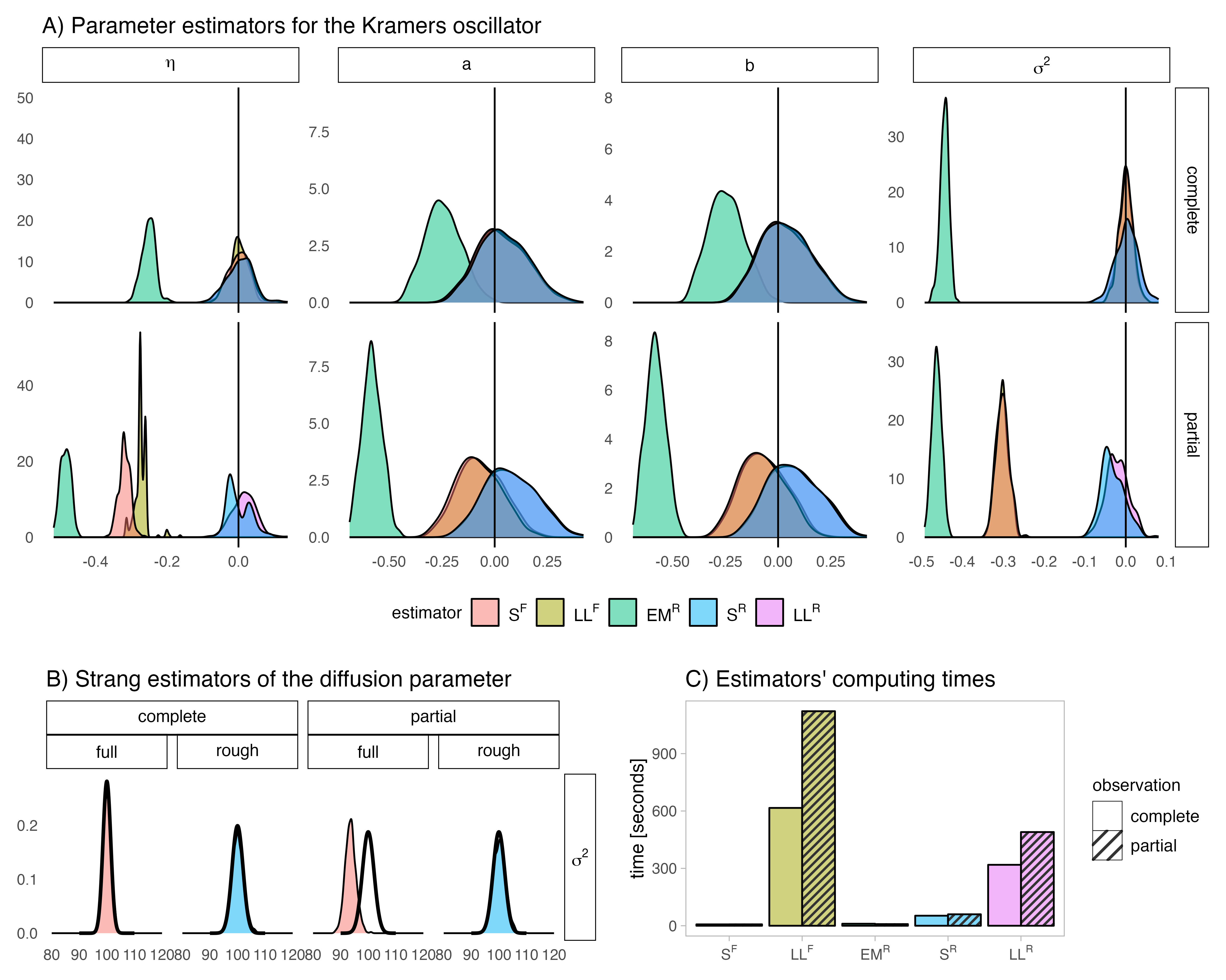
Figure 1: Parameter estimates in a simulation study for the Kramers oscillator, eq. (8). The color code remains consistent across all three figures. A) Normalized distributions of parameter estimation errors $(\hat{\bm{\theta}}_{N}-\bm{\theta}_{0})\oslash\bm{\theta}_{0}$ in both complete and partial observation cases, based on 250 simulated data sets with $h=0.1$ and $N=5000$. Each column corresponds to a different parameter, while the color indicates the type of estimator. Estimators are distinguished by superscripted objective functions ($\mathrm{F}$ for full and $\mathrm{R}$ for rough). B) Distribution of $\widehat{\sigma}_{N}^{2}$ estimators based on 1000 simulations with $h=0.02$ and $N=5000$ across different observation settings (complete or partial) and likelihood choices (full or rough) using the Strang splitting scheme. The true value of $\sigma^{2}$ is set to $\sigma_{0}^{2}=100$. Theoretical normal densities are overlaid for comparison. Theoretical variances are calculated based on $C_{\sigma^{2}}(\bm{\theta}_{0})$, eq. (52). C) Median computing time in seconds for one estimation of various estimators based on 250 simulations with $h=0.1$ and $N=5000$. Shaded color patterns represent times in the partial observation case, while no color pattern indicates times in the complete observation case.

4.4 Results

The results of the simulation study are presented in Figure 1. Figure 1A) presents the distributions of the normalized estimators in the complete and partial observation cases. The S and LL estimators exhibit nearly identical performance, particularly in the complete observation scenario. In contrast, the EM method displays significant underperformance and notable bias. The variances of the S and LL rough-likelihood estimators of $\sigma^{2}$ are higher compared to those derived from the full likelihood, aligning with theoretical expectations. Interestingly, in the partial observation scenario, Figure 1A) reveals that estimators employing the full likelihood display greater finite sample bias compared to those based on the rough likelihood. Possible reasons for this bias are discussed in Remark 3. However, it is noteworthy that this bias is eliminated for smaller time steps, e.g. $h=0.0001$ (not shown), thus confirming the theoretical asymptotic results. This observation suggests that the rough likelihood is preferable under partial observations due to its lower bias. Backward finite difference approximations of the velocity variables perform similarly to the forward differences and are therefore excluded from the figure for clarity.

We closely examine the variances of the S estimators of $\sigma^{2}$ in Figure 1B). The LL estimators are omitted due to their similarity to the S estimators, and because the computation times for the LL estimators are prohibitive. To align more closely with the asymptotic predictions, we opt for $h=0.02$ and conduct 1000 simulations. Additionally, we set $\sigma_{0}^{2}=100$ to test different noise levels. Atop each empirical distribution, we overlay theoretical normal densities that match the variances as per Theorem 3.2. The theoretical variance is derived from $C_{\sigma^{2}}(\bm{\theta}_{0})$ in (51), which for the Kramers oscillator in (8) is:

$$C_{\sigma^{2}}(\bm{\theta}_{0})=\frac{1}{\sigma_{0}^{4}}.$$ (52)

Figure 1 illustrates that the lowest variance of the diffusion estimator is observed when using the full likelihood with complete observations. The second lowest variance is achieved using the rough likelihood with complete observations. The largest variance is observed in the partial observation case; however, it remains independent of whether the full or rough likelihood is used. Once again, we observe that using the full likelihood introduces additional finite sample bias.

In Figure 1C), we compare running times calculated using the tictoc package in R. Running times are measured from the start of the optimization step until convergence. The figure depicts the median over 250 repetitions to mitigate the influence of outliers. The EM method is notably the fastest; however, the S estimators exhibit only slightly slower performance. The LL estimators are 10-100 times slower than the S estimators, depending on whether complete or partial observations are used and whether the full or rough likelihood is employed.

5 Application to Greenland Ice Core Data

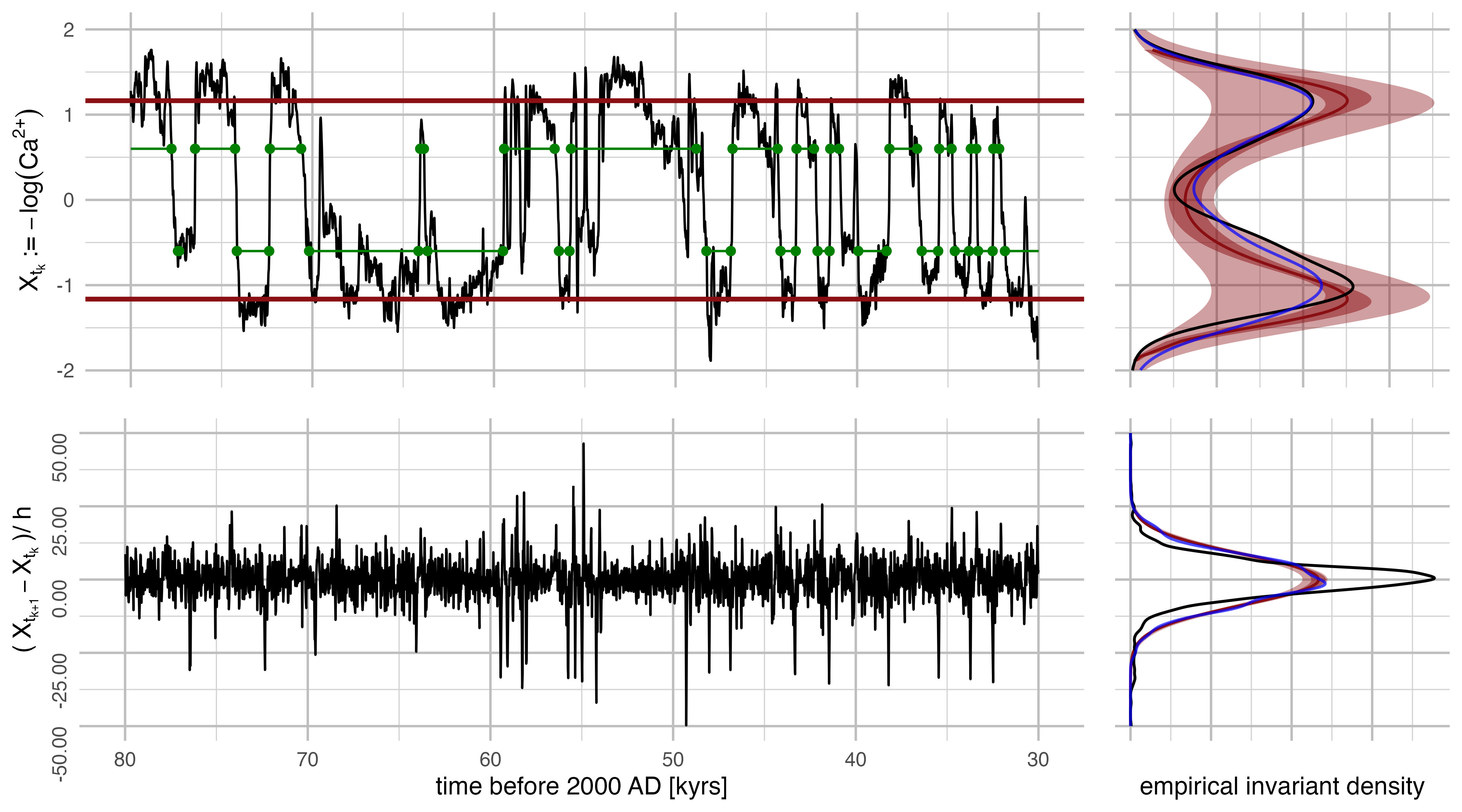
Figure 2: Ice core data from Greenland. Left: Trajectories over time (in kilo years) of the centered negative logarithm of the $\text{Ca}^{2+}$ measurements (top) and forward difference approximations of its rate of change (bottom). The two vertical dark red lines represent the estimated stable equilibria of the double-well potential function. Green points denote up- and down-crossings of level $\pm 0.6$, conditioned on having crossed the other level. Green vertical lines indicate empirical estimates of occupancy in either of the two metastable states. Right: Empirical densities (black) alongside estimated invariant densities with confidence intervals (dark red), prediction intervals (light red), and the empirical density of a simulated sample from the estimated model (blue).

During the last glacial period, significant climatic shifts known as Dansgaard-Oeschger (DO) events have been documented in paleoclimatic records (Dansgaard et al., 1993). Proxy data from Greenland ice cores, particularly stable water isotope composition ($\delta^{18}\text{O}$) and calcium ion concentrations ($\text{Ca}^{2+}$), offer valuable insights into these past climate variations (Boers et al., 2017, 2018; Boers, 2018; Ditlevsen et al., 2002; Lohmann and Ditlevsen, 2019; Hassanibesheli et al., 2020).

The $\delta^{18}\text{O}$ ratio, reflecting the relative abundance of ${}^{18}\text{O}$ and ${}^{16}\text{O}$ isotopes in ice, serves as a proxy for paleotemperatures during snow deposition. Conversely, calcium ions, originating from dust deposition, exhibit a strong negative correlation with $\delta^{18}\text{O}$, with higher calcium ion levels indicating colder conditions. Here, we prioritize $\text{Ca}^{2+}$ time series due to its finer temporal resolution.

In Greenland ice core records, the DO events manifest as abrupt transitions from colder climates (stadials) to approximately 10 degrees warmer climates (interstadials) within a few decades. Although the waiting times between state switches last a couple of thousand years, their spacing exhibits significant variability. The underlying mechanisms driving these changes remain largely elusive, prompting discussions on whether they follow cyclic patterns, result from external forcing, or emerge from noise-induced processes (Boers, 2018; Ditlevsen et al., 2007). We aim to determine if the observed data can be explained by noise-induced transitions of the Kramers oscillator.

The measurements were conducted at the summit of the Greenland ice sheet as part of the Greenland Icecore Project (GRIP) (Anklin et al., 1993; Andersen et al., 2004). Originally, the data were sampled at 5 cm intervals, resulting in a non-equidistant time series due to ice compression at greater depths, where 5 cm of ice core spans longer time periods. For our analysis, we use a version of the data transformed into a uniformly spaced series through 20-year binning and averaging. This transformation simplifies the analysis and highlights significant climatic trends. The dataset is available in the supplementary material of (Rasmussen et al., 2014; Seierstad et al., 2014).

To address the large amplitudes and negative correlation with temperature, we transform the data to minus the logarithm of $\text{Ca}^{2+}$, where higher values of the transformed variable indicate warmer climates at the time of snow deposition. Additionally, we center the transformed measurements around zero. With the 20-year binning, to obtain one point per 20 years, we average across the bins, resulting in a time step of $h=0.02\mathrm{kyr}$ ($1\mathrm{kyr}=1000$ years). Additionally, we addressed a few missing values using the na.approx function from the zoo package. Following the approach of Hassanibesheli et al. (2020), we analyze a subset of the data with a sufficiently good signal-to-noise ratio. Hassanibesheli et al. (2020) examined the data from $30$ to $60\mathrm{kyr}$ before present. Here, we extend the analysis to cover $30\mathrm{kyr}$ to $80\mathrm{kyr}$, resulting in a time interval of $T=50\mathrm{kyr}$ and a sample size of $N=2500$. We approximate the velocity of the transformed $\text{Ca}^{2+}$ by the forward difference method. The trajectories and empirical invariant distributions are illustrated in Figure 2.

We fit the Kramers oscillator to the $-\log\text{Ca}^{2+}$ time series and estimate parameters using the Strang estimator. Following Theorem 3.2, we compute $\mathbf{C}_{\bm{\beta}}(\bm{\theta}_{0})$ from (50). Applying the invariant density $\pi_{0}(x,v)$ from (10), which decouples into $\pi_{0}(x)$ (11) and a Gaussian zero-mean and $\sigma_{0}^{2}/(2\eta_{0})$ variance, leads us to:

$$\mathbf{C}_{\bm{\beta}}(\bm{\theta}_{0})=\begin{bmatrix}\frac{1}{2\eta_{0}}&0&0\\ \vspace{1ex}0&\frac{1}{\sigma_{0}^{2}}\int_{-\infty}^{\infty}x^{2}\pi_{0}(x)\operatorname*{\mathrm{d}\!}x&-\frac{1}{\sigma_{0}^{2}}\int_{-\infty}^{\infty}x^{4}\pi_{0}(x)\operatorname*{\mathrm{d}\!}x\\ 0&-\frac{1}{\sigma_{0}^{2}}\int_{-\infty}^{\infty}x^{4}\pi_{0}(x)\operatorname*{\mathrm{d}\!}x&\frac{1}{\sigma_{0}^{2}}\int_{-\infty}^{\infty}x^{6}\pi_{0}(x)\operatorname*{\mathrm{d}\!}x\end{bmatrix}.$$ (53)

Thus, to obtain $95\%$ confidence intervals (CI) for the estimated parameters, we plug $\widehat{\bm{\theta}}_{N}$ into (52) and (53). The estimators and confidence intervals are shown in Table 1. We also calculate the expected waiting time $\tau$, eq. (12), of crossing from one state to another, and its confidence interval using the Delta Method.

Parameter	Estimate	95% CI
$\eta$	62.5	$59.4-65.6$
$a$	296.7	$293.6-299.8$
$b$	219.1	$156.4-281.7$
$\sigma^{2}$	9125	$8589-9662$
$\tau$	3.97	$3.00-4.94$

Table 1: Estimated parameters of the Kramers oscillator from Greenland ice core data.

The model fit is assessed in the right panels of Figure 2. Here, we present the empirical distributions of the two coordinates along with the fitted theoretical invariant distribution and a $95\%$ confidence interval. Additionally, a prediction interval for the distribution is provided by simulating 1000 datasets from the fitted model, matching the size of the empirical data. We estimate the empirical distributions for each simulated dataset and construct a $95\%$ prediction interval using the pointwise 2.5th and 97.5th percentiles of these estimates. A single example trace is included in blue. While the fitted distribution for $-\log\text{Ca}^{2+}$ appears to fit well, even with this symmetric model, the velocity variables are not adequately captured. This discrepancy is likely due to the presence of extreme values in the data that are not effectively accounted for by additive Gaussian noise. Consequently, the model compensates by estimating a large variance.

We estimate the waiting time between metastable states to be approximately 4000 years. However, this approximation relies on certain assumptions, namely $62.5\approx\eta\gg\sqrt{a}\approx 17.2$ and $73\approx\sigma^{2}/2\eta\ll a^{2}/4b\approx 100$. Thus, the accuracy of the approximation may not be highly accurate.

Defining the current state of the process is not straightforward. One method involves identifying successive up- and down-crossings of predefined thresholds within the smoothed data. However, the estimated occupancy time in each state depends on the level of smoothing applied and the distance of crossing thresholds from zero. Using a smoothing technique involving running averages within windows of 11 data points (equivalent to 220 years) and detecting down- and up-crossings of levels $\pm 0.6$, we find an average occupancy time of 4058 years in stadial states and 3550 years in interstadial states. Nevertheless, the actual occupancy times exhibit significant variability, ranging from 60 to 6900 years, with the central $50\%$ of values falling between 665 and 2115 years. This classification of states is depicted in green in Figure 2. Overall, the estimated mean occupancy time inferred from the Kramers oscillator appears reasonable.

6 Technical results

In this Section, we present all the necessary technical properties that are used to derive the main results of the paper.

We start by expanding $\widetilde{\bm{\Omega}}_{h}$ and its block components $\bm{\Omega}_{h}^{\mathrm{[RR]}}(\bm{\theta})^{-1},\bm{\Omega}_{h}^{\mathrm{[S\mid R]}}(\bm{\theta})^{-1}$, $\log\det\bm{\Omega}_{h}^{\mathrm{[RR]}}(\bm{\theta}),\log\det\bm{\Omega}_{h}^{\mathrm{[S\mid R]}}(\bm{\theta})$ and $\log|\det D{\bm{f}}_{h/2}\left(\mathbf{y};\bm{\beta}\right)|$ when $h$ goes to zero. Then, we expand $\widetilde{\mathbf{Z}}_{k,k-1}(\bm{\beta})$ and $\widetilde{\overline{\mathbf{Z}}}_{k+1,k,k-1}(\bm{\beta})$ around $\mathbf{Y}_{t_{k-1}}$ when $h$ goes to zero. The main tools used are Itô’s lemma, Taylor expansions, and Fubini’s theorem. The final result is stated in Propositions 6.6 and 6.7. The approximations depend on the drift function $\mathbf{F}$, the nonlinear part $\mathbf{N}$, and some correlated sequences of Gaussian random variables. Finally, we obtain approximations of the objective functions (25), (30), (31) and (39) - (41). Proofs of all the stated propositions and lemmas in this section are in Supplementary Material S1.

6.1 Covariance matrix $\widetilde{\bm{\Omega}}_{h}$

The covariance matrix $\widetilde{\bm{\Omega}}_{h}$ is approximated by:

$$\widetilde{\bm{\Omega}}_{h} =\int_{0}^{h}e^{\widetilde{\mathbf{A}}(h-u)}\widetilde{\bm{\Sigma}}\widetilde{\bm{\Sigma}}^{\top}e^{\widetilde{\mathbf{A}}^{\top}(h-u)}\operatorname*{\mathrm{d}\!}u$$

$$=h\widetilde{\bm{\Sigma}}\widetilde{\bm{\Sigma}}^{\top}+\frac{h^{2}}{2}(\widetilde{\mathbf{A}}\widetilde{\bm{\Sigma}}\widetilde{\bm{\Sigma}}^{\top}+\widetilde{\bm{\Sigma}}\widetilde{\bm{\Sigma}}^{\top}\widetilde{\mathbf{A}}^{\top})+\frac{h^{3}}{6}(\widetilde{\mathbf{A}}^{2}\widetilde{\bm{\Sigma}}\widetilde{\bm{\Sigma}}^{\top}+2\widetilde{\mathbf{A}}\widetilde{\bm{\Sigma}}\widetilde{\bm{\Sigma}}^{\top}\widetilde{\mathbf{A}}^{\top}+\widetilde{\bm{\Sigma}}\widetilde{\bm{\Sigma}}^{\top}(\widetilde{\mathbf{A}}^{2})^{\top})$$

$$+\frac{h^{4}}{24}(\widetilde{\mathbf{A}}^{3}\widetilde{\bm{\Sigma}}\widetilde{\bm{\Sigma}}^{\top}+3\widetilde{\mathbf{A}}^{2}\widetilde{\bm{\Sigma}}\widetilde{\bm{\Sigma}}^{\top}\widetilde{\mathbf{A}}^{\top}+3\widetilde{\mathbf{A}}\widetilde{\bm{\Sigma}}\widetilde{\bm{\Sigma}}^{\top}(\widetilde{\mathbf{A}}^{2})^{\top}+\widetilde{\bm{\Sigma}}\widetilde{\bm{\Sigma}}^{\top}(\widetilde{\mathbf{A}}^{3})^{\top})+\mathbf{R}(h^{5},\mathbf{y}_{0}).$$ (54)

The following lemma approximates each block of $\widetilde{\bm{\Omega}}_{h}$ up to the first two leading orders of $h$. The result follows directly from equations (4), (6), and (54).

Lemma 6.1

The covariance matrix $\widetilde{\bm{\Omega}}_{h}$ defined in (54)-(19) approximates block-wise as:

$$\bm{\Omega}_{h}^{\mathrm{[SS]}}(\bm{\theta}) =\frac{h^{3}}{3}\bm{\Sigma}\bm{\Sigma}^{\top}+\frac{h^{4}}{8}(\mathbf{A}_{\mathbf{v}}(\bm{\beta})\bm{\Sigma}\bm{\Sigma}^{\top}+\bm{\Sigma}\bm{\Sigma}^{\top}\mathbf{A}_{\mathbf{v}}(\bm{\beta})^{\top})+\mathbf{R}(h^{5},\mathbf{y}_{0}),$$

$$\bm{\Omega}_{h}^{\mathrm{[SR]}}(\bm{\theta}) =\frac{h^{2}}{2}\bm{\Sigma}\bm{\Sigma}^{\top}+\frac{h^{3}}{6}(\mathbf{A}_{\mathbf{v}}(\bm{\beta})\bm{\Sigma}\bm{\Sigma}^{\top}+2\bm{\Sigma}\bm{\Sigma}^{\top}\mathbf{A}_{\mathbf{v}}(\bm{\beta})^{\top})+\mathbf{R}(h^{4},\mathbf{y}_{0}),$$

$$\bm{\Omega}_{h}^{\mathrm{[RS]}}(\bm{\theta}) =\frac{h^{2}}{2}\bm{\Sigma}\bm{\Sigma}^{\top}+\frac{h^{3}}{6}(2\mathbf{A}_{\mathbf{v}}(\bm{\beta})\bm{\Sigma}\bm{\Sigma}^{\top}+\bm{\Sigma}\bm{\Sigma}^{\top}\mathbf{A}_{\mathbf{v}}(\bm{\beta})^{\top})+\mathbf{R}(h^{4},\mathbf{y}_{0}),$$

$$\bm{\Omega}_{h}^{\mathrm{[RR]}}(\bm{\theta}) =h\bm{\Sigma}\bm{\Sigma}^{\top}+\frac{h^{2}}{2}(\mathbf{A}_{\mathbf{v}}(\bm{\beta})\bm{\Sigma}\bm{\Sigma}^{\top}+\bm{\Sigma}\bm{\Sigma}^{\top}\mathbf{A}_{\mathbf{v}}(\bm{\beta})^{\top})+\mathbf{R}(h^{3},\mathbf{y}_{0}).$$

Building on Lemma 6.1, we calculate products, inverses, and logarithms of the components of $\widetilde{\bm{\Omega}}_{h}$ in the following lemma.

Lemma 6.2

For the covariance matrix $\widetilde{\bm{\Omega}}_{h}$ defined in (54) it holds:

1. $\bm{\Omega}_{h}^{\mathrm{[RR]}}(\bm{\theta})^{-1}=\frac{1}{h}(\bm{\Sigma}\bm{\Sigma}^{\top})^{-1}-\frac{1}{2}((\bm{\Sigma}\bm{\Sigma}^{\top})^{-1}\mathbf{A}_{\mathbf{v}}(\bm{\beta})+\mathbf{A}_{\mathbf{v}}(\bm{\beta})^{\top}(\bm{\Sigma}\bm{\Sigma}^{\top})^{-1})+\mathbf{R}(h,\mathbf{y}_{0})$;

2. $\bm{\Omega}_{h}^{\mathrm{[SR]}}(\bm{\theta})\bm{\Omega}_{h}^{\mathrm{[RR]}}(\bm{\theta})^{-1}=\frac{h}{2}\mathbf{I}-\frac{h^{2}}{12}(\mathbf{A}_{\mathbf{v}}-\bm{\Sigma}\bm{\Sigma}^{\top}\mathbf{A}_{\mathbf{v}}(\bm{\beta})^{\top}(\bm{\Sigma}\bm{\Sigma}^{\top})^{-1})+\mathbf{R}(h^{3},\mathbf{y}_{0})$;

3. $\bm{\Omega}_{h}^{\mathrm{[SR]}}(\bm{\theta})\bm{\Omega}_{h}^{\mathrm{[RR]}}(\bm{\theta})^{-1}\bm{\Omega}_{h}^{\mathrm{[RS]}}(\bm{\theta})=\frac{h^{3}}{4}\bm{\Sigma}\bm{\Sigma}^{\top}+\frac{h^{4}}{8}(\mathbf{A}_{\mathbf{v}}(\bm{\beta})\bm{\Sigma}\bm{\Sigma}^{\top}+\bm{\Sigma}\bm{\Sigma}^{\top}\mathbf{A}_{\mathbf{v}}(\bm{\beta})^{\top})+\mathbf{R}(h^{5},\mathbf{y}_{0})$;

4. $\bm{\Omega}_{h}^{\mathrm{[S\mid R]}}(\bm{\theta})=\frac{h^{3}}{12}\bm{\Sigma}\bm{\Sigma}^{\top}+\mathbf{R}(h^{5},\mathbf{y}_{0})$;

5. $\log\det\bm{\Omega}_{h}^{\mathrm{[RR]}}(\bm{\theta})=d\log h+\log\det\bm{\Sigma}\bm{\Sigma}^{\top}+h\operatorname*{Tr}\mathbf{A}_{\mathbf{v}}(\bm{\beta})+{R}(h^{2},\mathbf{y}_{0})$;

6. $\log\det\bm{\Omega}_{h}^{\mathrm{[S\mid R]}}(\bm{\theta})=3d\log h+\log\det\bm{\Sigma}\bm{\Sigma}^{\top}+{R}(h^{2},\mathbf{y}_{0})$;

7. $\log\det\widetilde{\bm{\Omega}}_{h}(\bm{\theta})=4d\log h+2\log\det\bm{\Sigma}\bm{\Sigma}^{\top}+h\operatorname*{Tr}\mathbf{A}_{\mathbf{v}}(\bm{\beta})+{R}(h^{2},\mathbf{y}_{0})$.

Remark 5

We adjusted the objective functions for partial observations using the term $c\log\det\bm{\Omega}_{h/c}^{\mathrm{[\cdot]}}$, where $c$ is a correction constant. This adjustment keeps the term $h\operatorname*{Tr}\mathbf{A}_{\mathbf{v}}(\bm{\beta})$ in (v)-(vii) constant, not affecting the asymptotic distribution of the drift parameter. There is no $h^{4}$-term in $\bm{\Omega}_{h}^{\mathrm{[S\mid R]}}(\bm{\theta})$ which simplifies the approximation of $\bm{\Omega}_{h}^{\mathrm{[S\mid R]}}(\bm{\theta})^{-1}$ and $\log\det\bm{\Omega}_{h}^{\mathrm{[S\mid R]}}(\bm{\theta})$. Consequently, this makes (41) a bad choice for estimating the drift parameter.

6.2 Nonlinear solution $\widetilde{\bm{f}}_{h}$

We now state a useful proposition for the nonlinear solution $\widetilde{\bm{f}}_{h}$ (Section 1.8 in (Hairer et al., 1993)).

Proposition 6.3

Let Assumptions (A1), (A2) and (A6) hold. When $h\to 0$, the $h$-flow of (15) approximates as:

$$\widetilde{\bm{f}}_{h}(\mathbf{y}) =\mathbf{y}+h\widetilde{\mathbf{N}}(\mathbf{y})+\frac{h^{2}}{2}(D_{\mathbf{y}}\widetilde{\mathbf{N}}(\mathbf{y}))\widetilde{\mathbf{N}}(\mathbf{y})+\mathbf{R}(h^{3},\mathbf{y}),$$ (55)

$$\widetilde{\bm{f}}_{h}^{-1}(\mathbf{y}) =\mathbf{y}-h\widetilde{\mathbf{N}}(\mathbf{y})+\frac{h^{2}}{2}(D_{\mathbf{y}}\widetilde{\mathbf{N}}(\mathbf{y}))\widetilde{\mathbf{N}}(\mathbf{y})+\mathbf{R}(h^{3},\mathbf{y}).$$ (56)

Applying the previous proposition on (21) and (22), we get:

$$\bm{f}_{h}(\mathbf{y}) =\mathbf{v}+h\mathbf{N}(\mathbf{y})+\frac{h^{2}}{2}(D_{\mathbf{v}}\mathbf{N}(\mathbf{y}))\mathbf{N}(\mathbf{y})+\mathbf{R}(h^{3},\mathbf{y}),$$ (57)

$$\bm{f}^{\star-1}_{h}(\mathbf{y}) =\mathbf{v}-h\mathbf{N}(\mathbf{y})+\frac{h^{2}}{2}(D_{\mathbf{v}}\mathbf{N}(\mathbf{y}))\mathbf{N}(\mathbf{y})+\mathbf{R}(h^{3},\mathbf{y}).$$ (58)

The following lemma approximates $\log|\det D{\bm{f}}_{h/2}\left(\mathbf{y};\bm{\beta}\right)|$ in the objective functions and connects it with Lemma 6.2.

Lemma 6.4

Let $\widetilde{\bm{f}}_{h}$ be the function defined in (21). It holds:

$$2\log|\det D{\bm{f}}_{h/2}\left(\mathbf{Y}_{t_{k}};\bm{\beta}\right)| =h\operatorname*{Tr}D_{\mathbf{v}}{\mathbf{N}}(\mathbf{Y}_{t_{k-1}};\bm{\beta})+{R}(h^{3/2},\mathbf{Y}_{t_{k-1}}),$$

$$2\log|\det D{\bm{f}}_{h/2}\left(\mathbf{X}_{t_{k}},\Delta_{h}\mathbf{X}_{t_{k+1}};\bm{\beta}\right)| =h\operatorname*{Tr}D_{\mathbf{v}}{\mathbf{N}}(\mathbf{Y}_{t_{k-1}};\bm{\beta})+{R}(h^{3/2},\mathbf{Y}_{t_{k-1}}).$$

An immediate consequence of the previous lemma and that $D_{\mathbf{v}}\mathbf{F}(\mathbf{y};\bm{\beta})=\mathbf{A}_{\mathbf{v}}(\bm{\beta})+D_{\mathbf{v}}\mathbf{N}(\mathbf{y};\bm{\beta})$ is

$$\log\det\bm{\Omega}_{h}^{\mathrm{[RR]}}(\bm{\theta})+2\log|\det D{\bm{f}}_{h/2}\left(\mathbf{Y}_{t_{k}};\bm{\beta}\right)| =\log\det h\bm{\Sigma}\bm{\Sigma}^{\top}+h\operatorname*{Tr}D_{\mathbf{v}}\mathbf{F}(\mathbf{Y}_{t_{k-1}};\bm{\beta})+R(h^{3/2},\mathbf{Y}_{t_{k-1}}).$$

The same equality holds when $\mathbf{Y}_{t_{k}}$ is approximated by $(\mathbf{X}_{t_{k}},\Delta_{h}\mathbf{X}_{t_{k+1}})$. The following lemma expands function $\bm{\mu}_{h}(\widetilde{\bm{f}}_{h/2}(\mathbf{y}))$ up to the highest necessary order of $h$.

Lemma 6.5

For the functions $\widetilde{\bm{f}}_{h}$ in (21) and $\widetilde{\bm{\mu}}_{h}$ in (28), it holds

$$\bm{\mu}_{h}^{\mathrm{[S]}}(\widetilde{\bm{f}}_{h/2}(\mathbf{y})) =\mathbf{x}+h\mathbf{v}+\frac{h^{2}}{2}\mathbf{F}(\mathbf{y})+\mathbf{R}(h^{3},\mathbf{y}),$$ (59)

$$\bm{\mu}_{h}^{\mathrm{[R]}}(\widetilde{\bm{f}}_{h/2}(\mathbf{y})) =\mathbf{v}+h(\mathbf{F}(\mathbf{y})-\frac{1}{2}\mathbf{N}(\mathbf{y}))+\mathbf{R}(h^{2},\mathbf{y}).$$ (60)

6.3 Random variables $\widetilde{\mathbf{Z}}_{k,k-1}$ and $\widetilde{\overline{\mathbf{Z}}}_{k+1,k,k-1}$

To approximate the random variables $\mathbf{Z}_{k,k-1}^{\mathrm{[S]}}(\bm{\beta}),\mathbf{Z}_{k,k-1}^{\mathrm{[R]}}(\bm{\beta})$, $\overline{\mathbf{Z}}_{k,k-1}^{[\mathrm{S}]}(\bm{\beta})$, and $\overline{\mathbf{Z}}_{k+1,k,k-1}^{[\mathrm{R}]}(\bm{\beta})$ around $\mathbf{Y}_{t_{k-1}}$, we start by defining the following random sequences:

$$\bm{\eta}_{k-1} \coloneqq\frac{1}{h^{1/2}}\int_{t_{k-1}}^{t_{k}}\operatorname*{\mathrm{d}\!}\mathbf{W}_{t},$$ (61)

$$\bm{\xi}_{k-1} \coloneqq\frac{1}{h^{3/2}}\int_{t_{k-1}}^{t_{k}}(t-t_{k-1})\operatorname*{\mathrm{d}\!}\mathbf{W}_{t}, \bm{\xi}_{k}^{\prime}\coloneqq\frac{1}{h^{3/2}}\int_{t_{k}}^{t_{k+1}}(t_{k+1}-t)\operatorname*{\mathrm{d}\!}\mathbf{W}_{t},$$ (62)

$$\bm{\zeta}_{k-1} \coloneqq\frac{1}{h^{5/2}}\int_{t_{k-1}}^{t_{k}}(t-t_{k-1})^{2}\operatorname*{\mathrm{d}\!}\mathbf{W}_{t}, \bm{\zeta}_{k}^{\prime}\coloneqq\frac{1}{h^{5/2}}\int_{t_{k}}^{t_{k+1}}(t_{k+1}-t)^{2}\operatorname*{\mathrm{d}\!}\mathbf{W}_{t}.$$ (63)

The random variables (61)-(63) are Gaussian with mean zero. Moreover, at time $t_{k}$ they are $\mathcal{F}_{t_{k+1}}$ measurable and independent of $\mathcal{F}_{t_{k}}$. The following linear combinations of (61)-(63) appear in the expansions in the partial observation case:

$$\mathbf{U}_{k,k-1} \coloneqq\bm{\xi}_{k}^{\prime}+\bm{\xi}_{k-1},$$ (64)

$$\mathbf{Q}_{k,k-1} \coloneqq\bm{\zeta}_{k}^{\prime}+2\bm{\eta}_{k-1}-\bm{\zeta}_{k-1}.$$ (65)

It is not hard to check that $\bm{\xi}_{k}^{\prime}+\bm{\eta}_{k-1}-\bm{\xi}_{k-1}^{\prime}=\mathbf{U}_{k,k-1}$. This alternative representation of $\mathbf{U}_{k,k-1}$ will be used later in proofs.

The Itô isometry yields:

$$\mathbb{E}_{\bm{\theta}_{0}}[\bm{\eta}_{k-1}\bm{\eta}_{k-1}^{\top}\mid\mathcal{F}_{t_{k-1}}] =\mathbf{I}, \mathbb{E}_{\bm{\theta}_{0}}[\bm{\eta}_{k-1}\bm{\xi}_{k-1}^{\top}\mid\mathcal{F}_{t_{k-1}}]=\mathbb{E}_{\bm{\theta}_{0}}[\bm{\eta}_{k-1}\bm{\xi}_{k-1}^{\prime\top}\mid\mathcal{F}_{t_{k-1}}]=\frac{1}{2}\mathbf{I},$$ (66)

$$\mathbb{E}_{\bm{\theta}_{0}}[\bm{\xi}_{k-1}\bm{\xi}_{k-1}^{\prime\top}\mid\mathcal{F}_{t_{k-1}}] =\frac{1}{6}\mathbf{I}, \mathbb{E}_{\bm{\theta}_{0}}[\bm{\xi}_{k-1}\bm{\xi}_{k-1}^{\top}\mid\mathcal{F}_{t_{k-1}}]=\mathbb{E}_{\bm{\theta}_{0}}[\bm{\xi}_{k}^{\prime}\bm{\xi}_{k}^{\prime\top}\mid\mathcal{F}_{t_{k-1}}]=\frac{1}{3}\mathbf{I},$$ (67)

$$\mathbb{E}_{\bm{\theta}_{0}}[\mathbf{U}_{k,k-1}\mathbf{U}_{k,k-1}^{\top}\mid\mathcal{F}_{t_{k-1}}] =\frac{2}{3}\mathbf{I}, \mathbb{E}_{\bm{\theta}_{0}}[\mathbf{U}_{k,k-1}(\mathbf{U}_{k,k-1}+2\bm{\xi}_{k-1}^{\prime})^{\top}\mid\mathcal{F}_{t_{k-1}}]=\mathbf{I}.$$ (68)

The covariances of other combinations of the random variables (61)-(63) are not needed for the proofs. However, to derive asymptotic properties, we need some fourth moments calculated in Supplementary Materials S1.

The following two propositions are the last building blocks for approximating the objective functions (30)-(31) and (40)-(41).

Proposition 6.6

The random variables $\widetilde{\mathbf{Z}}_{k,k-1}(\bm{\beta})$ in (24) and $\widetilde{\overline{\mathbf{Z}}}_{k+1,k,k-1}(\bm{\beta})$ in (35) are approximated by:

$$\mathbf{Z}_{k,k-1}^{\mathrm{[S]}}(\bm{\beta}) =h^{3/2}\bm{\Sigma}_{0}\bm{\xi}^{\prime}_{k-1}+\frac{h^{2}}{2}(\mathbf{F}_{0}(\mathbf{Y}_{t_{k-1}})-\mathbf{F}(\mathbf{Y}_{t_{k-1}}))+\frac{h^{5/2}}{2}D_{\mathbf{v}}\mathbf{F}_{0}(\mathbf{Y}_{t_{k-1}})\bm{\Sigma}_{0}\bm{\zeta}^{\prime}_{k-1}+\mathbf{R}(h^{3},\mathbf{Y}_{t_{k-1}}),$$

$$\mathbf{Z}_{k,k-1}^{\mathrm{[R]}}(\bm{\beta}) =h^{1/2}\bm{\Sigma}_{0}\bm{\eta}_{k-1}+h(\mathbf{F}_{0}(\mathbf{Y}_{t_{k-1}})-\mathbf{F}(\mathbf{Y}_{t_{k-1}}))-\frac{h^{3/2}}{2}D_{\mathbf{v}}\mathbf{N}(\mathbf{Y}_{t_{k-1}})\bm{\Sigma}_{0}\bm{\eta}_{k-1}$$

$$+h^{3/2}D_{\mathbf{v}}\mathbf{F}_{0}(\mathbf{Y}_{t_{k-1}})\bm{\Sigma}_{0}\bm{\xi}^{\prime}_{k-1}+\mathbf{R}(h^{2},\mathbf{Y}_{t_{k-1}}),$$

$$\overline{\mathbf{Z}}_{k,k-1}^{[\mathrm{S}]}(\bm{\beta}) =-\frac{h^{2}}{2}\mathbf{F}(\mathbf{Y}_{t_{k-1}})-\frac{h^{5/2}}{2}D_{\mathbf{v}}\mathbf{F}(\mathbf{Y}_{t_{k-1}})\bm{\Sigma}_{0}\bm{\xi}^{\prime}_{k-1}+\mathbf{R}(h^{3},\mathbf{Y}_{t_{k-1}}),$$

$$\overline{\mathbf{Z}}_{k+1,k,k-1}^{[\mathrm{R}]}(\bm{\beta}) =h^{1/2}\bm{\Sigma}_{0}\mathbf{U}_{k,k-1}+h(\mathbf{F}_{0}(\mathbf{Y}_{t_{k-1}})-\mathbf{F}(\mathbf{Y}_{t_{k-1}}))-\frac{h^{3/2}}{2}D_{\mathbf{v}}\mathbf{N}(\mathbf{Y}_{t_{k-1}})\bm{\Sigma}_{0}\mathbf{U}_{k,k-1}$$

$$-h^{3/2}D_{\mathbf{v}}\mathbf{F}(\mathbf{Y}_{t_{k-1}})\bm{\Sigma}_{0}\bm{\xi}_{k-1}^{\prime}+\frac{h^{3/2}}{2}D_{\mathbf{v}}\mathbf{F}_{0}(\mathbf{Y}_{t_{k-1}})\bm{\Sigma}_{0}\mathbf{Q}_{k,k-1}+\mathbf{R}(h^{2},\mathbf{Y}_{t_{k-1}}).$$

Remark 6

Proposition 6.6 yield

$$\mathbb{E}_{\bm{\theta}_{0}}[\mathbf{Z}_{k,k-1}^{\mathrm{[R]}}(\bm{\beta})\mathbf{Z}_{k,k-1}^{\mathrm{[R]}}(\bm{\beta})^{\top}\mid\mathbf{Y}_{t_{k-1}}] =h\bm{\Sigma}\bm{\Sigma}_{0}^{\top}+\mathbf{R}(h^{2},\mathbf{Y}_{t_{k-1}})=\bm{\Omega}_{h}^{\mathrm{[RR]}}+\mathbf{R}(h^{2},\mathbf{Y}_{t_{k-1}}),$$

$$\mathbb{E}_{\bm{\theta}_{0}}[\overline{\mathbf{Z}}_{k+1,k,k-1}^{\mathrm{[R]}}(\bm{\beta})\overline{\mathbf{Z}}_{k+1,k,k-1}^{\mathrm{[R]}}(\bm{\beta})^{\top}\mid\mathbf{Y}_{t_{k-1}}] =\frac{2}{3}h\bm{\Sigma}\bm{\Sigma}_{0}^{\top}+\mathbf{R}(h^{2},\mathbf{Y}_{t_{k-1}})=\frac{2}{3}\bm{\Omega}_{h}^{\mathrm{[RR]}}+\mathbf{R}(h^{2},\mathbf{Y}_{t_{k-1}}).$$

Thus, the correction factor $2/3$ in (40) compensates for the underestimation of the covariance of $\overline{\mathbf{Z}}_{k+1,k,k-1}^{\mathrm{[R]}}(\bm{\beta})$. Similarly, it can be shown that the same underestimation happens when using the backward difference. On the other hand, when using the central difference, it can be shown that

$$\mathbb{E}_{\bm{\theta}_{0}}[\overline{\mathbf{Z}}_{k+1,k,k-1}^{\mathrm{[R]},central}(\bm{\beta})\overline{\mathbf{Z}}_{k+1,k,k-1}^{\mathrm{[R]},central}(\bm{\beta})^{\top}\mid\mathbf{Y}_{t_{k-1}}] =\frac{5}{12}h\bm{\Sigma}\bm{\Sigma}_{0}^{\top}+\mathbf{R}(h^{2},\mathbf{Y}_{t_{k-1}}),$$

which is a larger deviation from $\bm{\Omega}_{h}^{\mathrm{[RR]}}$, yielding a larger correcting factor and larger asymptotic variance of the diffusion parameter estimator.

Proposition 6.7

Let $\widetilde{\mathbf{Z}}_{k,k-1}(\bm{\beta})$ and $\widetilde{\overline{\mathbf{Z}}}_{k+1,k,k-1}(\bm{\beta})$ be defined in (24) and (35), respectively. Then,

$$\mathbf{Z}_{k,k-1}^{\mathrm{[S\mid R]}}(\bm{\beta}) =-\frac{h^{3/2}}{2}\bm{\Sigma}_{0}(\bm{\eta}_{k-1}-2\bm{\xi}^{\prime}_{k-1})+\frac{h^{5/2}}{12}(\mathbf{A}_{\mathbf{v}}-\bm{\Sigma}\bm{\Sigma}^{\top}\mathbf{A}_{\mathbf{v}}(\bm{\beta})^{\top}(\bm{\Sigma}\bm{\Sigma}^{\top})^{-1})\bm{\Sigma}_{0}\bm{\eta}_{k-1}$$

$$+\frac{h^{5/2}}{4}D_{\mathbf{v}}\mathbf{N}(\mathbf{Y}_{t_{k-1}})\bm{\Sigma}_{0}\bm{\eta}_{k-1}-\frac{h^{5/2}}{2}D_{\mathbf{v}}\mathbf{F}_{0}(\mathbf{Y}_{t_{k-1}})\bm{\Sigma}_{0}(\bm{\xi}^{\prime}_{k-1}-\bm{\zeta}^{\prime}_{k-1})+\mathbf{R}(h^{3},\mathbf{Y}_{t_{k-1}}),$$

$$\overline{\mathbf{Z}}_{k+1,k,k-1}^{\mathrm{[S\mid R]}}(\bm{\beta}) =-\frac{h^{3/2}}{2}\bm{\Sigma}_{0}\mathbf{U}_{k,k-1}-\frac{h^{2}}{2}\mathbf{F}_{0}(\mathbf{Y}_{t_{k-1}})+\frac{h^{5/2}}{12}(\mathbf{A}_{\mathbf{v}}-\bm{\Sigma}\bm{\Sigma}^{\top}\mathbf{A}_{\mathbf{v}}(\bm{\beta})^{\top}(\bm{\Sigma}\bm{\Sigma}^{\top})^{-1})\bm{\Sigma}_{0}\mathbf{U}_{k,k-1}$$

$$+\frac{h^{5/2}}{4}D_{\mathbf{v}}\mathbf{N}(\mathbf{Y}_{t_{k-1}})\bm{\Sigma}_{0}\mathbf{U}_{k,k-1}-\frac{h^{5/2}}{4}D_{\mathbf{v}}\mathbf{F}_{0}(\mathbf{Y}_{t_{k-1}})\bm{\Sigma}_{0}\mathbf{Q}_{k,k-1}+\mathbf{R}(h^{3},\mathbf{Y}_{t_{k-1}}).$$

6.4 Objective functions

Starting with the complete observation case, we approximate objective functions (30) and (31) up to order $R(h^{3/2},\mathbf{Y}_{t_{k-1}})$ to prove the asymptotic properties of the estimators $\hat{\bm{\theta}}_{N}^{\mathrm{[CR]}}$ and $\hat{\bm{\theta}}_{N}^{\mathrm{[CS\mid R]}}$. After omitting the terms of order $R(h,\mathbf{Y}_{t_{k-1}})$ that do not depend on $\bm{\beta}$, we obtain the following approximations:

$$\mathcal{L}_{N}^{\mathrm{[CR]}} \left(\mathbf{Y}_{0:t_{N}};\bm{\theta}\right)=(N-1)\log\det\bm{\Sigma}\bm{\Sigma}^{\top}+\sum_{k=1}^{N}\bm{\eta}_{k-1}^{\top}\bm{\Sigma}_{0}^{\top}(\bm{\Sigma}\bm{\Sigma}^{\top})^{-1}\bm{\Sigma}_{0}\bm{\eta}_{k-1}$$ (69)

$$+2\sqrt{h}\sum_{k=1}^{N}\bm{\eta}_{k-1}^{\top}\bm{\Sigma}_{0}^{\top}(\bm{\Sigma}\bm{\Sigma}^{\top})^{-1}(\mathbf{F}(\mathbf{Y}_{t_{k-1}};\bm{\beta}_{0})-\mathbf{F}(\mathbf{Y}_{t_{k-1}};\bm{\beta}))$$

$$+h\sum_{k=1}^{N}(\mathbf{F}(\mathbf{Y}_{t_{k-1}};\bm{\beta}_{0})-\mathbf{F}(\mathbf{Y}_{t_{k-1}};\bm{\beta}))^{\top}(\bm{\Sigma}\bm{\Sigma}^{\top})^{-1}(\mathbf{F}(\mathbf{Y}_{t_{k-1}};\bm{\beta}_{0})-\mathbf{F}(\mathbf{Y}_{t_{k-1}};\bm{\beta}))$$

$$-h\sum_{k=1}^{N}\bm{\eta}_{k-1}^{\top}\bm{\Sigma}_{0}^{\top}D_{\mathbf{v}}\mathbf{F}(\mathbf{Y}_{t_{k-1}};\bm{\beta})^{\top}(\bm{\Sigma}\bm{\Sigma}^{\top})^{-1}\bm{\Sigma}_{0}\bm{\eta}_{k-1}+h\sum_{k=1}^{N}\operatorname*{Tr}D_{\mathbf{v}}\mathbf{F}(\mathbf{Y}_{t_{k}};\bm{\beta}),$$

$$\mathcal{L}_{N}^{\mathrm{[CS\mid R]}} \left(\mathbf{Y}_{0:t_{N}};\bm{\theta}\right)=(N-1)\log\det\bm{\Sigma}\bm{\Sigma}^{\top}+3\sum_{k=1}^{N}(\bm{\eta}_{k-1}-2\bm{\xi}^{\prime}_{k-1})^{\top}\bm{\Sigma}_{0}^{\top}(\bm{\Sigma}\bm{\Sigma}^{\top})^{-1}\bm{\Sigma}_{0}(\bm{\eta}_{k-1}-2\bm{\xi}^{\prime}_{k-1})$$ (70)

$$-3h\sum_{k=1}^{N}(\bm{\eta}_{k-1}-2\bm{\xi}^{\prime}_{k-1})^{\top}\bm{\Sigma}_{0}^{\top}(\bm{\Sigma}\bm{\Sigma}^{\top})^{-1}D_{\mathbf{v}}\mathbf{N}(\mathbf{Y}_{t_{k-1}};\bm{\beta})\bm{\Sigma}_{0}\bm{\eta}_{k-1}$$

$$-h\sum_{k=1}^{N}(\bm{\eta}_{k-1}-2\bm{\xi}^{\prime}_{k-1})^{\top}\bm{\Sigma}_{0}^{\top}(\bm{\Sigma}\bm{\Sigma}^{\top})^{-1}(\mathbf{A}_{\mathbf{v}}(\bm{\beta})-\bm{\Sigma}\bm{\Sigma}^{\top}\mathbf{A}_{\mathbf{v}}(\bm{\beta})^{\top}(\bm{\Sigma}\bm{\Sigma}^{\top})^{-1})\bm{\Sigma}_{0}\bm{\eta}_{k-1}$$

$$\mathcal{L}_{N}^{\mathrm{[CF]}} \left(\mathbf{Y}_{0:t_{N}};\bm{\theta}\right)=\mathcal{L}_{N}^{\mathrm{[CR]}}\left(\mathbf{Y}_{0:t_{N}};\bm{\theta}\right)+\mathcal{L}_{N}^{\mathrm{[CS\mid R]}}\left(\mathbf{Y}_{0:t_{N}};\bm{\theta}\right).$$ (71)

The two last sums in (70) converge to zero because $\mathbb{E}_{\bm{\theta}_{0}}[(\bm{\eta}_{k-1}-2\bm{\xi}^{\prime}_{k-1})\bm{\eta}_{k-1}^{\top}|\mathcal{F}_{t_{k-1}}]=\mathbf{0}$. Moreover, (70) lacks the quadratic form of $\mathbf{F}(\mathbf{Y}_{t_{k-1}})-\mathbf{F}_{0}(\mathbf{Y}_{t_{k-1}})$, that is crucial for the asymptotic variance of the drift estimator. This implies that the objective function $\mathcal{L}_{N}^{\mathrm{[CS\mid R]}}$ is not suitable for estimating the drift parameter. Conversely, (70) provides a correct and consistent estimator of the diffusion parameter, indicating that the full objective function (the sum of $\mathcal{L}_{N}^{\mathrm{[CR]}}$ and $\mathcal{L}_{N}^{\mathrm{[CS\mid R]}}$) consistently estimates $\bm{\theta}$.

Similarly, the approximated objective functions in the partial observation case are:

$$\mathcal{L}_{N}^{\mathrm{[PR]}} \left(\mathbf{Y}_{0:t_{N}};\bm{\theta}\right)=\frac{2}{3}(N-2)\log\det\bm{\Sigma}\bm{\Sigma}^{\top}+\sum_{k=1}^{N-1}\mathbf{U}_{k,k-1}^{\top}\bm{\Sigma}_{0}^{\top}(\bm{\Sigma}\bm{\Sigma}^{\top})^{-1}\bm{\Sigma}_{0}\mathbf{U}_{k,k-1}$$ (72)

$$+2\sqrt{h}\sum_{k=1}^{N}\mathbf{U}_{k,k-1}^{\top}\bm{\Sigma}_{0}^{\top}(\bm{\Sigma}\bm{\Sigma}^{\top})^{-1}(\mathbf{F}(\mathbf{Y}_{t_{k-1}};\bm{\beta}_{0})-\mathbf{F}(\mathbf{Y}_{t_{k-1}};\bm{\beta}))$$

$$+h\sum_{k=1}^{N-1}(\mathbf{F}(\mathbf{Y}_{t_{k-1}};\bm{\beta}_{0})-\mathbf{F}(\mathbf{Y}_{t_{k-1}};\bm{\beta}))^{\top}(\bm{\Sigma}\bm{\Sigma}^{\top})^{-1}(\mathbf{F}(\mathbf{Y}_{t_{k-1}};\bm{\beta}_{0})-\mathbf{F}(\mathbf{Y}_{t_{k-1}};\bm{\beta}))$$

$$-h\sum_{k=1}^{N-1}(\mathbf{U}_{k,k-1}+2\bm{\xi}_{k-1}^{\prime})^{\top}\bm{\Sigma}_{0}^{\top}D_{\mathbf{v}}\mathbf{F}(\mathbf{Y}_{t_{k-1}};\bm{\beta})^{\top}(\bm{\Sigma}\bm{\Sigma}^{\top})^{-1}\bm{\Sigma}_{0}\mathbf{U}_{k,k-1}+h\sum_{k=1}^{N-1}\operatorname*{Tr}D_{\mathbf{v}}\mathbf{F}(\mathbf{Y}_{t_{k}};\bm{\beta}),$$

$$\mathcal{L}_{N}^{\mathrm{[PS\mid R]}} \left(\mathbf{Y}_{0:t_{N}};\bm{\theta}\right)=2(N-2)\log\det\bm{\Sigma}\bm{\Sigma}^{\top}+3\sum_{k=1}^{N-1}\mathbf{U}_{k,k-1}^{\top}\bm{\Sigma}_{0}^{\top}(\bm{\Sigma}\bm{\Sigma}^{\top})^{-1}\bm{\Sigma}_{0}\mathbf{U}_{k,k-1}$$ (73)

$$+6\sqrt{h}\sum_{k=1}^{N}\mathbf{U}_{k,k-1}^{\top}\bm{\Sigma}_{0}^{\top}(\bm{\Sigma}\bm{\Sigma}^{\top})^{-1}\mathbf{F}(\mathbf{Y}_{t_{k-1}};\bm{\beta}_{0})$$

$$-3h\sum_{k=1}^{N-1}\mathbf{U}_{k,k-1}^{\top}\bm{\Sigma}_{0}^{\top}D_{\mathbf{v}}\mathbf{N}(\mathbf{Y}_{t_{k-1}};\bm{\beta})^{\top}(\bm{\Sigma}\bm{\Sigma}^{\top})^{-1}\bm{\Sigma}_{0}\mathbf{U}_{k,k-1}+2h\sum_{k=1}^{N-1}\operatorname*{Tr}D_{\mathbf{v}}\mathbf{N}(\mathbf{Y}_{t_{k}};\bm{\beta}),$$

$$\mathcal{L}_{N}^{\mathrm{[PF]}} \left(\mathbf{Y}_{0:t_{N}};\bm{\theta}\right)=\mathcal{L}_{N}^{\mathrm{[PR]}}\left(\mathbf{Y}_{0:t_{N}};\bm{\theta}\right)+\mathcal{L}_{N}^{\mathrm{[PS\mid R]}}\left(\mathbf{Y}_{0:t_{N}};\bm{\theta}\right).$$ (74)

This time, the term with $\mathbf{A}_{\mathbf{v}}(\bm{\beta})-\bm{\Sigma}\bm{\Sigma}^{\top}\mathbf{A}_{\mathbf{v}}(\bm{\beta})^{\top}(\bm{\Sigma}\bm{\Sigma}^{\top})^{-1}$ vanishes because

$$\operatorname*{Tr}(\bm{\Sigma}_{0}\mathbf{U}_{k,k-1}\mathbf{U}_{k,k-1}^{\top}\bm{\Sigma}_{0}^{\top}(\bm{\Sigma}\bm{\Sigma}^{\top})^{-1}(\mathbf{A}_{\mathbf{v}}(\bm{\beta})-\bm{\Sigma}\bm{\Sigma}^{\top}\mathbf{A}_{\mathbf{v}}(\bm{\beta})^{\top}(\bm{\Sigma}\bm{\Sigma}^{\top})^{-1}))=0$$

due to the symmetry of the matrices and the trace cyclic property.

Even though the partial observation objective function $\mathcal{L}^{\mathrm{[PR]}}\left(\mathbf{X}_{0:t_{N}};\bm{\theta}\right)$ (40) depends only on $\mathbf{X}_{0:t_{N}}$, we could approximate it with $\mathcal{L}_{N}^{\mathrm{[PR]}}\left(\mathbf{Y}_{0:t_{N}};\bm{\theta}\right)$ (72). This is useful for proving the asymptotic normality of the estimator since its asymptotic distribution will depend on the invariant probability $\nu_{0}$ defined for the solution $\mathbf{Y}$.

The absence of the quadratic form $\mathbf{F}(\mathbf{Y}_{t_{k-1}})-\mathbf{F}_{0}(\mathbf{Y}_{t_{k-1}})$ in (73) indicates that $\mathcal{L}_{N}^{\mathrm{[PS\mid R]}}$ is not suitable for estimating the drift parameter. Additionally, the penultimate term in (73) does not vanish, needing an additional correction term of $2h\sum_{k=1}^{N-1}\operatorname*{Tr}D_{\mathbf{v}}\mathbf{N}(\mathbf{Y}_{t_{k}};\bm{\beta})$ for consistency. This correction is represented as $4\log|\det D_{\mathbf{v}}\bm{f}_{h/2}|$ in (41). Notably, this term is absent in the complete objective function (31), making this adjustment somewhat artificial and could potentially deviate further from the true log-likelihood. Consequently, the objective function based on the full likelihood (39) inherits this characteristic from (73), suggesting that in the partial observation scenario, using only the rough likelihood (72) may be more appropriate.

7 Conclusion

Many fundamental laws of physics and chemistry are formulated as second-order differential equations, a model class important for understanding complex dynamical systems in various fields such as biology and economics. The extension of these deterministic models to stochastic second-order differential equations represents a natural generalization, allowing for the incorporation of uncertainties and variability inherent in real-world systems. However, robust statistical methods for analyzing data generated from such stochastic models have been lacking, presenting a significant challenge due to the inherent degeneracy of the noise and partial observation.

In this study, we propose estimating model parameters using a recently developed methodology of Strang splitting estimator for SDEs. This estimator has demonstrated finite sample efficiency with relatively large sample time steps, particularly in handling highly nonlinear models. We adjust the estimator to the partial observation setting and employ either the full likelihood or only the marginal likelihood based on the rough coordinates. For all four obtained estimators, we establish the consistency and asymptotic normality.

The application of the Strang estimator to a historical paleoclimate dataset obtained from ice cores in Greenland has yielded valuable insights and analytical tools for comprehending abrupt climate shifts throughout history. Specifically, we employed the stochastic Duffing oscillator, also known as the Kramers oscillator, to analyze the data.

While our focus in this paper has been primarily confined to second-order SDEs with no parameters in the smooth components, we are confident that our findings can be extended to encompass models featuring parameters in the drift of the smooth coordinates. This opens up directions for further exploration and application of our methodology to a broader range of complex dynamical systems, promising deeper insights into their behavior and underlying mechanisms.

S1 Supplementary Material

In this section, we provide proofs for all the nontrivial lemmas, propositions, and theorems presented in Sections 3 and 6. The majority of these proofs, especially those in Section 6, heavily rely on Itô or Taylor expansions in $h$ around $\mathbf{Y}_{t_{k-1}}$. Additionally, we frequently employ Fubini’s theorem as a useful tool. Our initial focus is on the results from Section 6, as they constitute technical auxiliary properties essential for understanding the main results outlined in Section 3.

S1.1 Proofs of results from Section 6

• To prove (i), calculate

  $$\bm{\Omega}_{h}^{\mathrm{[RR]}}(\bm{\theta})^{-1} =\frac{1}{h}(\bm{\Sigma}\bm{\Sigma}^{\top})^{-1}(\mathbf{I}+\frac{h}{2}(\mathbf{A}_{\mathbf{v}}(\bm{\beta})+\bm{\Sigma}\bm{\Sigma}^{\top}\mathbf{A}_{\mathbf{v}}(\bm{\beta})^{\top}(\bm{\Sigma}\bm{\Sigma}^{\top})^{-1})^{-1})+\mathbf{R}(h,\mathbf{y}_{0})$$

  $$=\frac{1}{h}(\bm{\Sigma}\bm{\Sigma}^{\top})^{-1}(\mathbf{I}-\frac{h}{2}(\mathbf{A}_{\mathbf{v}}(\bm{\beta})+\bm{\Sigma}\bm{\Sigma}^{\top}\mathbf{A}_{\mathbf{v}}(\bm{\beta})^{\top}(\bm{\Sigma}\bm{\Sigma}^{\top})^{-1})+\mathbf{R}(h,\mathbf{y}_{0})$$

  $$=\frac{1}{h}(\bm{\Sigma}\bm{\Sigma}^{\top})^{-1}-\frac{1}{2}((\bm{\Sigma}\bm{\Sigma}^{\top})^{-1}\mathbf{A}_{\mathbf{v}}(\bm{\beta})+\mathbf{A}_{\mathbf{v}}(\bm{\beta})^{\top}(\bm{\Sigma}\bm{\Sigma}^{\top})^{-1})+\mathbf{R}(h,\mathbf{y}_{0}).$$

  Proof of (ii):

  $$\bm{\Omega}_{h}^{\mathrm{[SR]}}(\bm{\theta})\bm{\Omega}_{h}^{\mathrm{[RR]}}(\bm{\theta})^{-1} =(\frac{h^{2}}{2}(\bm{\Sigma}\bm{\Sigma}^{\top})+\frac{h^{3}}{6}(\mathbf{A}_{\mathbf{v}}(\bm{\beta})(\bm{\Sigma}\bm{\Sigma}^{\top})+2\bm{\Sigma}\bm{\Sigma}^{\top}\mathbf{A}_{\mathbf{v}}(\bm{\beta})^{\top}))\frac{1}{h}(\bm{\Sigma}\bm{\Sigma}^{\top})^{-1}$$

  $$-\frac{h^{2}}{4}(\bm{\Sigma}\bm{\Sigma}^{\top})((\bm{\Sigma}\bm{\Sigma}^{\top})^{-1}\mathbf{A}_{\mathbf{v}}(\bm{\beta})+\mathbf{A}_{\mathbf{v}}(\bm{\beta})^{\top}(\bm{\Sigma}\bm{\Sigma}^{\top})^{-1}))+\mathbf{R}(h^{3},\mathbf{y}_{0})$$

  $$=\frac{h}{2}\mathbf{I}-\frac{h^{2}}{12}(\mathbf{A}_{\mathbf{v}}-\bm{\Sigma}\bm{\Sigma}^{\top}\mathbf{A}_{\mathbf{v}}(\bm{\beta})^{\top}(\bm{\Sigma}\bm{\Sigma}^{\top})^{-1})+\mathbf{R}(h^{3},\mathbf{y}_{0}).$$

  To prove (iii), use the previous result to obtain:

  $$\bm{\Omega}_{h}^{\mathrm{[SR]}}(\bm{\theta})\bm{\Omega}_{h}^{\mathrm{[RR]}}(\bm{\theta})^{-1}\bm{\Omega}_{h}^{\mathrm{[RS]}}(\bm{\theta})$$

  $$=(\frac{h}{2}\mathbf{I}-\frac{h^{2}}{12}(\mathbf{A}_{\mathbf{v}}-\bm{\Sigma}\bm{\Sigma}^{\top}\mathbf{A}_{\mathbf{v}}(\bm{\beta})^{\top}(\bm{\Sigma}\bm{\Sigma}^{\top})^{-1}))(\frac{h^{2}}{2}(\bm{\Sigma}\bm{\Sigma}^{\top})+\frac{h^{3}}{6}(2\mathbf{A}_{\mathbf{v}}(\bm{\beta})(\bm{\Sigma}\bm{\Sigma}^{\top})+\bm{\Sigma}\bm{\Sigma}^{\top}\mathbf{A}_{\mathbf{v}}(\bm{\beta})^{\top}))+\mathbf{R}(h^{5},\mathbf{y}_{0})$$

  $$=\frac{h^{3}}{4}\bm{\Sigma}\bm{\Sigma}^{\top}+\frac{h^{4}}{8}(\mathbf{A}_{\mathbf{v}}(\bm{\beta})\bm{\Sigma}\bm{\Sigma}^{\top}+\bm{\Sigma}\bm{\Sigma}^{\top}\mathbf{A}_{\mathbf{v}}(\bm{\beta})^{\top})+\mathbf{R}(h^{5},\mathbf{y}_{0}).$$

  Proof of (iv) follows from (iii) and Lemma 6.1. To prove (v), approximate the log-determinant as:

  $$\log\det\bm{\Omega}_{h}^{\mathrm{[RR]}}(\bm{\theta}) =\log\det\left(h\bm{\Sigma}\bm{\Sigma}^{\top}+\frac{h^{2}}{2}(\mathbf{A}_{\mathbf{v}}(\bm{\beta})\bm{\Sigma}\bm{\Sigma}^{\top}+\bm{\Sigma}\bm{\Sigma}^{\top}\mathbf{A}_{\mathbf{v}}(\bm{\beta})^{\top})\right)+{R}(h^{2},\mathbf{y}_{0})$$

  $$=d\log h+\log\det\bm{\Sigma}\bm{\Sigma}^{\top}+\log\det\left(\mathbf{I}+\frac{h}{2}(\mathbf{A}_{\mathbf{v}}(\bm{\beta})+\bm{\Sigma}\bm{\Sigma}^{\top}\mathbf{A}_{\mathbf{v}}(\bm{\beta})^{\top}(\bm{\Sigma}\bm{\Sigma}^{\top})^{-1})\right)+{R}(h^{2},\mathbf{y}_{0})$$

  $$=d\log h+\log\det\bm{\Sigma}\bm{\Sigma}^{\top}+\frac{h}{2}\operatorname*{Tr}(\mathbf{A}_{\mathbf{v}}(\bm{\beta})+\bm{\Sigma}\bm{\Sigma}^{\top}\mathbf{A}_{\mathbf{v}}(\bm{\beta})^{\top}(\bm{\Sigma}\bm{\Sigma}^{\top})^{-1})+{R}(h^{2},\mathbf{y}_{0})$$

  $$=d\log h+\log\det\bm{\Sigma}\bm{\Sigma}^{\top}+h\operatorname*{Tr}\mathbf{A}_{\mathbf{v}}(\bm{\beta})+{R}(h^{2},\mathbf{y}_{0}).$$ (S1)

  To prove (vi), repeat the previous reasoning on (iv). The proof of (vii) follows from $\det\widetilde{\bm{\Omega}}_{h}=\det\bm{\Omega}_{h}^{\mathrm{[RR]}}\det\bm{\Omega}_{h}^{\mathrm{[S\mid R]}}$ and properties (v) and (vi).

• Using the same approximation as in the previous proof of (v), we obtain:

  $$2\log|\det D{\bm{f}}_{h/2}\left(\mathbf{y};\bm{\beta}\right)| =2\log|\det(\mathbf{I}+\frac{h}{2}D{\mathbf{N}}(\mathbf{y};\bm{\beta}))|+{R}(h^{2},\mathbf{y})$$

  $$=2\log|1+\frac{h}{2}\operatorname*{Tr}D{\mathbf{N}}(\mathbf{y};\bm{\beta})|+{R}(h^{2},\mathbf{y})$$

  $$=h\operatorname*{Tr}D{\mathbf{N}}(\mathbf{y};\bm{\beta})+{R}(h^{2},\mathbf{y})=h\operatorname*{Tr}D_{\mathbf{v}}{\mathbf{N}}(\mathbf{y};\bm{\beta})+{R}(h^{2},\mathbf{y}).$$ (S2)

  In complete observation, put $\mathbf{Y}_{t_{k}}$ instead of $\mathbf{y}$ and use Itô’s lemma on $\mathbf{N}(\mathbf{Y}_{t_{k}})$ as in (S6). In partial observation, put $(\mathbf{X}_{t_{k}},\Delta_{h}\mathbf{X}_{t_{k+1}})$ instead of $\mathbf{y}$ and approximate $\mathbf{N}(\mathbf{X}_{t_{k}},\Delta_{h}\mathbf{X}_{t_{k+1}})$ as in (S7).

• We use definition (6) and approximation (55), and plug them in (17) to obtain:

  $$\widetilde{\bm{\mu}}_{h}(\widetilde{\bm{f}}_{h/2}(\mathbf{y})) =e^{\widetilde{\mathbf{A}}h}(\widetilde{\boldsymbol{f}}_{h/2}(\mathbf{y})-\widetilde{\mathbf{b}})+\widetilde{\mathbf{b}}$$

  $$=\left(\mathbf{I}_{2d}+h\widetilde{\mathbf{A}}+\frac{h^{2}}{2}\widetilde{\mathbf{A}}^{2}+\mathbf{R}(h^{3},\mathbf{y})\right)(\widetilde{\boldsymbol{f}}_{h/2}(\mathbf{y})-\widetilde{\mathbf{b}})+\widetilde{\mathbf{b}}$$

  $$=\begin{bmatrix}\mathbf{I}_{d}+\frac{h^{2}}{2}\mathbf{A}_{\mathbf{x}}+\mathbf{R}(h^{3},\mathbf{y})&h\mathbf{I}_{d}+\frac{h^{2}}{2}\mathbf{A}_{\mathbf{v}}+\mathbf{R}(h^{3},\mathbf{y})\vspace{1ex}\\ h\mathbf{A}_{\mathbf{x}}+\mathbf{R}(h^{2},\mathbf{y})&\mathbf{I}_{d}+h\mathbf{A}_{\mathbf{v}}+\mathbf{R}(h^{2},\mathbf{y})\end{bmatrix}\begin{bmatrix}\mathbf{x}-\mathbf{b}\\ \mathbf{v}+\frac{h}{2}\mathbf{N}(\mathbf{y})+\mathbf{R}(h^{2},\mathbf{y})\end{bmatrix}+\begin{bmatrix}\mathbf{b}\\ \mathbf{0}\end{bmatrix}$$

  $$=\begin{bmatrix}\mathbf{x}+h\mathbf{v}+\frac{h^{2}}{2}\mathbf{F}(\mathbf{y})+\mathbf{R}(h^{3},\mathbf{y})\vspace{1ex}\\ \mathbf{v}+h(\mathbf{F}(\mathbf{y})-\frac{1}{2}\mathbf{N}(\mathbf{y}))+\mathbf{R}(h^{2},\mathbf{y})\end{bmatrix}.$$

  This concludes the proof.

To prove Proposition 6.6, we need the following lemma that provides expansion of $\Delta_{h}\mathbf{X}_{t_{k+1}}-\Delta_{h}\mathbf{X}_{t_{k}}$.

Lemma S1.1

For process $\Delta_{h}\mathbf{X}_{t_{k+1}}$ (33) it holds:

$$\Delta_{h}\mathbf{X}_{t_{k+1}}-\Delta_{h}\mathbf{X}_{t_{k}} =\sqrt{h}\bm{\Sigma}_{0}\mathbf{U}_{k,k-1}+h\mathbf{F}_{0}(\mathbf{Y}_{t_{k-1}})+\frac{h^{3/2}}{2}D_{\mathbf{v}}\mathbf{F}_{0}(\mathbf{Y}_{t_{k-1}})\bm{\Sigma}_{0}\mathbf{Q}_{k,k-1}+\mathbf{R}(h^{2},\mathbf{Y}_{t_{k-1}}),$$ (S3)

$$\Delta_{h}\mathbf{X}_{t_{k}}-\mathbf{V}_{t_{k-1}} =\sqrt{h}\bm{\Sigma}_{0}\bm{\xi}_{k-1}^{\prime}+\frac{h}{2}\mathbf{F}_{0}(\mathbf{Y}_{t_{k-1}})+\frac{h^{3/2}}{2}D_{\mathbf{v}}\mathbf{F}_{0}(\mathbf{Y}_{t_{k-1}})\bm{\Sigma}_{0}\bm{\zeta}^{\prime}_{k-1}+\mathbf{R}(h^{2},\mathbf{Y}_{t_{k-1}}).$$ (S4)

• Proof of (S3). Equation (2) in integral form and (33) yield:

  $$\Delta_{h}\mathbf{X}_{t_{k+1}}-\Delta_{h}\mathbf{X}_{t_{k}} =\frac{1}{h}\int_{t_{k}}^{t_{k+1}}\mathbf{V}_{t}\operatorname*{\mathrm{d}\!}t-\frac{1}{h}\int_{t_{k-1}}^{t_{k}}\mathbf{V}_{t}\operatorname*{\mathrm{d}\!}t=\frac{1}{h}\int_{t_{k}}^{t_{k+1}}(\mathbf{V}_{t}-\mathbf{V}_{t_{k}})\operatorname*{\mathrm{d}\!}t+\frac{1}{h}\int_{t_{k-1}}^{t_{k}}(\mathbf{V}_{t_{k}}-\mathbf{V}_{t})\operatorname*{\mathrm{d}\!}t$$

  $$=\frac{1}{h}\int_{t_{k}}^{t_{k+1}}\int_{t_{k}}^{t}\mathbf{F}_{0}(\mathbf{Y}_{s})\operatorname*{\mathrm{d}\!}s\operatorname*{\mathrm{d}\!}t+\frac{1}{h}\bm{\Sigma}_{0}\int_{t_{k}}^{t_{k+1}}\int_{t_{k}}^{t}\operatorname*{\mathrm{d}\!}\mathbf{W}_{s}\operatorname*{\mathrm{d}\!}t$$

  $$+\frac{1}{h}\int_{t_{k-1}}^{t_{k}}\int_{t}^{t_{k}}\mathbf{F}_{0}(\mathbf{Y}_{s})\operatorname*{\mathrm{d}\!}s\operatorname*{\mathrm{d}\!}t+\frac{1}{h}\bm{\Sigma}_{0}\int_{t_{k-1}}^{t_{k}}\int_{t}^{t_{k}}\operatorname*{\mathrm{d}\!}\mathbf{W}_{s}\operatorname*{\mathrm{d}\!}t.$$

  Apply Fubini’s theorem on double integrals to obtain:

  $$\Delta_{h}\mathbf{X}_{t_{k+1}}-\Delta_{h}\mathbf{X}_{t_{k}} =\frac{1}{h}\int_{t_{k}}^{t_{k+1}}(t_{k+1}-t)\mathbf{F}_{0}(\mathbf{Y}_{t})\operatorname*{\mathrm{d}\!}t+\frac{1}{h}\int_{t_{k-1}}^{t_{k}}(t-t_{k-1})\mathbf{F}_{0}(\mathbf{Y}_{t})\operatorname*{\mathrm{d}\!}t+\sqrt{h}\bm{\Sigma}_{0}\mathbf{U}_{k,k-1}.$$ (S5)

  Applying Itô’s lemma on $\mathbf{F}_{0}(\mathbf{Y}_{t})$ yields the following approximation:

  $$\mathbf{F}_{0}(\mathbf{Y}_{t}) =\mathbf{F}_{0}(\mathbf{Y}_{t_{k}})+D_{\mathbf{v}}\mathbf{F}_{0}(\mathbf{Y}_{t_{k}})\bm{\Sigma}_{0}\int_{t_{k}}^{t}\operatorname*{\mathrm{d}\!}\mathbf{W}_{s}+\mathbf{R}(h,\mathbf{Y}_{t_{k}}).$$ (S6)

  Plugging (S6) into (S5) gives:

  $$\Delta_{h}\mathbf{X}_{t_{k+1}}-\Delta_{h}\mathbf{X}_{t_{k}} =h\mathbf{F}_{0}(\mathbf{Y}_{t_{k}})+\frac{1}{h}D_{\mathbf{v}}\mathbf{F}_{0}(\mathbf{Y}_{t_{k}})\bm{\Sigma}_{0}\int_{t_{k}}^{t_{k+1}}\int_{t_{k}}^{t}(t_{k+1}-t)\operatorname*{\mathrm{d}\!}\mathbf{W}_{s}\operatorname*{\mathrm{d}\!}t$$

  $$-\frac{1}{h}D_{\mathbf{v}}\mathbf{F}_{0}(\mathbf{Y}_{t_{k}})\bm{\Sigma}_{0}\int_{t_{k-1}}^{t_{k}}\int_{t}^{t_{k}}(t-t_{k-1})\operatorname*{\mathrm{d}\!}\mathbf{W}_{s}\operatorname*{\mathrm{d}\!}t+\sqrt{h}\bm{\Sigma}_{0}\mathbf{U}_{k,k-1}+\mathbf{R}(h^{2},\mathbf{Y}_{t_{k-1}}).$$

  Once again, apply Fubini’s theorem on the double integrals to get:

  $$\int_{t_{k}}^{t_{k+1}}\int_{t_{k}}^{t}(t_{k+1}-t)\operatorname*{\mathrm{d}\!}\mathbf{W}_{s}\operatorname*{\mathrm{d}\!}t=\frac{1}{2}h^{5/2}\bm{\zeta}_{k}^{\prime},\qquad\int_{t_{k-1}}^{t_{k}}\int_{t}^{t_{k}}(t-t_{k-1})\operatorname*{\mathrm{d}\!}\mathbf{W}_{s}\operatorname*{\mathrm{d}\!}t=\frac{1}{2}h^{5/2}\bm{\zeta}_{k-1}.$$

  So far, we have

  $$\Delta_{h}\mathbf{X}_{t_{k+1}}-\Delta_{h}\mathbf{X}_{t_{k}} =\sqrt{h}\bm{\Sigma}_{0}\mathbf{U}_{k,k-1}+h\mathbf{F}_{0}(\mathbf{Y}_{t_{k}})+\frac{h^{3/2}}{2}D_{\mathbf{v}}\mathbf{F}_{0}(\mathbf{Y}_{t_{k}})\bm{\Sigma}_{0}(\bm{\zeta}^{\prime}_{k}-\bm{\zeta}_{k-1})+\mathbf{R}(h^{2},\mathbf{Y}_{t_{k-1}}).$$

  To conclude the proof, use Itô’s lemma to get $\mathbf{F}_{0}(\mathbf{Y}_{t_{k}})=\mathbf{F}_{0}(\mathbf{Y}_{t_{k-1}})+\sqrt{h}D_{\mathbf{v}}\mathbf{F}_{0}(\mathbf{Y}_{t_{k-1}})\bm{\Sigma}_{0}\bm{\eta}_{k-1}+\mathbf{R}(h,\mathbf{Y}_{t_{k-1}})$.

  Proof of (S4). As before, start with (33) and use (S6) to get:

  $$\Delta_{h}\mathbf{X}_{t_{k}}-\mathbf{V}_{t_{k-1}} =\frac{1}{h}\int_{t_{k-1}}^{t_{k}}(t_{k}-t)\mathbf{F}_{0}(\mathbf{Y}_{t})\operatorname*{\mathrm{d}\!}t+\frac{1}{h}\bm{\Sigma}_{0}\int_{t_{k-1}}^{t_{k}}(t_{k}-t)\operatorname*{\mathrm{d}\!}\mathbf{W}_{t}$$

  $$=\sqrt{h}\bm{\Sigma}_{0}\bm{\xi}_{k-1}^{\prime}+\frac{h}{2}\mathbf{F}_{0}(\mathbf{Y}_{t_{k-1}})+\frac{1}{h}D_{\mathbf{v}}\mathbf{F}_{0}(\mathbf{Y}_{t_{k}})\bm{\Sigma}_{0}\int_{t_{k-1}}^{t_{k}}\int_{t_{k-1}}^{t}(t_{k}-t)\operatorname*{\mathrm{d}\!}\mathbf{W}_{s}\operatorname*{\mathrm{d}\!}t+\mathbf{R}(h^{2},\mathbf{Y}_{t_{k-1}}).$$

  This concludes the proof.

• The expansion of $\mathbf{Z}_{k,k-1}^{\mathrm{[S]}}$ follows directly from Lemma 6.5 and S1.1. Indeed, it holds

  $$\mathbf{Z}_{k,k-1}^{\mathrm{[S]}}(\bm{\beta}) =\mathbf{X}_{t_{k}}-\mathbf{X}_{t_{k-1}}-h\mathbf{V}_{t_{k-1}}-\frac{h^{2}}{2}\mathbf{F}(\mathbf{Y}_{t_{k-1}})+\mathbf{R}(h^{3},\mathbf{Y}_{t_{k-1}})$$

  $$=h(\Delta_{h}\mathbf{X}_{t_{k}}-\mathbf{V}_{t_{k-1}})-\frac{h^{2}}{2}\mathbf{F}(\mathbf{Y}_{t_{k-1}})+\mathbf{R}(h^{3},\mathbf{Y}_{t_{k-1}}).$$

  To expand $\mathbf{Z}_{k,k-1}^{\mathrm{[R]}}$, we use definition (27) and approximations (58) and (60), as follows:

  $$\mathbf{Z}_{k,k-1}^{\mathrm{[R]}}(\bm{\beta}) =\mathbf{V}_{t_{k}}-\mathbf{V}_{t_{k-1}}-h\mathbf{F}(\mathbf{Y}_{t_{k-1}})-\frac{h}{2}(\mathbf{N}(\mathbf{Y}_{t_{k}})-\mathbf{N}(\mathbf{Y}_{t_{k-1}}))+\mathbf{R}(h^{2},\mathbf{Y}_{t_{k-1}})$$

  $$=\bm{\Sigma}_{0}\int_{t_{k-1}}^{t_{k}}\operatorname*{\mathrm{d}\!}\mathbf{W}_{t}+\int_{t_{k-1}}^{t_{k}}\mathbf{F}_{0}(\mathbf{Y}_{t})\operatorname*{\mathrm{d}\!}t-h\mathbf{F}(\mathbf{Y}_{t_{k-1}})-\frac{h}{2}(\mathbf{N}(\mathbf{Y}_{t_{k}})-\mathbf{N}(\mathbf{Y}_{t_{k-1}}))+\mathbf{R}(h^{2},\mathbf{Y}_{t_{k-1}})$$

  $$=\sqrt{h}\bm{\Sigma}_{0}\bm{\eta}_{k-1}+h(\mathbf{F}_{0}(\mathbf{Y}_{t_{k-1}})-\mathbf{F}(\mathbf{Y}_{t_{k-1}}))-\frac{h}{2}(\mathbf{N}(\mathbf{Y}_{t_{k}})-\mathbf{N}(\mathbf{Y}_{t_{k-1}}))$$

  $$+D_{\mathbf{v}}\mathbf{F}_{0}(\mathbf{Y}_{t_{k-1}})\bm{\Sigma}_{0}\int_{t_{k-1}}^{t_{k}}\int_{t_{k-1}}^{t}\operatorname*{\mathrm{d}\!}\mathbf{W}_{s}\operatorname*{\mathrm{d}\!}t+\mathbf{R}(h^{2},\mathbf{Y}_{t_{k-1}}).$$

  In the last line, we used Itô’s lemma on $\mathbf{F}_{0}(\mathbf{Y}_{t})$ as in (S6). Again, apply Itô’s lemma on $\mathbf{N}(\mathbf{Y}_{t_{k}})$ to get:

  $$\mathbf{Z}_{k,k-1}^{\mathrm{[R]}}(\bm{\beta}) =\sqrt{h}\bm{\Sigma}_{0}\bm{\eta}_{k-1}+h(\mathbf{F}_{0}(\mathbf{Y}_{t_{k-1}})-\mathbf{F}(\mathbf{Y}_{t_{k-1}}))-\frac{h^{3/2}}{2}D_{\mathbf{v}}\mathbf{N}(\mathbf{Y}_{t_{k-1}})\bm{\Sigma}_{0}\bm{\eta}_{k-1}$$

  $$+h^{3/2}D_{\mathbf{v}}\mathbf{F}_{0}(\mathbf{Y}_{t_{k-1}})\bm{\Sigma}_{0}\bm{\xi}^{\prime}_{k-1}+\mathbf{R}(h^{2},\mathbf{Y}_{t_{k-1}}).$$

  The expansion of $\mathbf{Z}_{k,k-1}^{\mathrm{[S]}}$ follows from definition (36) and plugging $(\mathbf{X}_{t_{k-1}},\Delta_{h}\mathbf{X}_{t_{k}})$ in approximation (60):

  $$\overline{\mathbf{Z}}_{k+1,k,k-1}^{[\mathrm{S}]}(\bm{\beta}) =\mathbf{X}_{t_{k}}-\mathbf{X}_{t_{k-1}}-h\Delta_{h}\mathbf{X}_{t_{k}}-\frac{h^{2}}{2}\mathbf{F}(\mathbf{X}_{t_{k-1}},\Delta_{h}\mathbf{X}_{t_{k}})+\mathbf{R}(h^{3},\mathbf{Y}_{t_{k-1}})$$

  $$=-\frac{h^{2}}{2}\mathbf{F}(\mathbf{X}_{t_{k-1}},\Delta_{h}\mathbf{X}_{t_{k}})+\mathbf{R}(h^{3},\mathbf{Y}_{t_{k-1}}).$$

  Use Taylor’s formula on $\mathbf{F}(\mathbf{X}_{t_{k-1}},\Delta_{h}\mathbf{X}_{t_{k}})$ to get

  $$\mathbf{F}(\mathbf{X}_{t_{k-1}},\Delta_{h}\mathbf{X}_{t_{k}}) =\mathbf{F}(\mathbf{Y}_{t_{k-1}})+D_{\mathbf{v}}\mathbf{F}(\mathbf{Y}_{t_{k-1}})(\Delta_{h}\mathbf{X}_{t_{k}}-\mathbf{V}_{t_{k-1}})+\mathbf{R}(h^{2},\mathbf{Y}_{t_{k-1}}).$$ (S7)

  Now, the rest follows from Lemma S1.1.

  Finally, to expand $\overline{\mathbf{Z}}_{k+1,k,k-1}^{[\mathrm{R}]}$, start with definition (37) and approximations (58), and (60):

  $$\overline{\mathbf{Z}}_{k+1,k,k-1}^{[\mathrm{R}]}(\bm{\beta}) =\Delta_{h}\mathbf{X}_{t_{k+1}}-\Delta_{h}\mathbf{X}_{t_{k}}-h\mathbf{F}(\mathbf{X}_{t_{k-1}},\Delta_{h}\mathbf{X}_{t_{k}})$$

  $$-\frac{h}{2}(\mathbf{N}(\mathbf{X}_{t_{k}},\Delta_{h}\mathbf{X}_{t_{k+1}})-\mathbf{N}(\mathbf{X}_{t_{k-1}},\Delta_{h}\mathbf{X}_{t_{k}}))+\mathbf{R}(h^{2},\mathbf{Y}_{t_{k-1}}).$$

  Lemma S1.1 yields:

  $$\overline{\mathbf{Z}}_{k+1,k,k-1}^{[\mathrm{R}]}(\bm{\beta}) =\sqrt{h}\bm{\Sigma}_{0}\mathbf{U}_{k,k-1}+h(\mathbf{F}_{0}(\mathbf{Y}_{t_{k-1}})-\mathbf{F}(\mathbf{X}_{t_{k-1}},\Delta_{h}\mathbf{X}_{t_{k}}))$$

  $$-\frac{h}{2}(\mathbf{N}(\mathbf{X}_{t_{k}},\Delta_{h}\mathbf{X}_{t_{k+1}})-\mathbf{N}(\mathbf{X}_{t_{k-1}},\Delta_{h}\mathbf{X}_{t_{k}}))+\frac{h^{3/2}}{2}D_{\mathbf{v}}\mathbf{F}_{0}(\mathbf{Y}_{t_{k-1}})\bm{\Sigma}_{0}\mathbf{Q}_{k,k-1}+\mathbf{R}(h^{2},\mathbf{Y}_{t_{k-1}}).$$

  Apply Taylor’s formula on $\mathbf{F}(\mathbf{X}_{t_{k-1}},\Delta_{h}\mathbf{X}_{t_{k}})$, $\mathbf{N}(\mathbf{X}_{t_{k}},\Delta_{h}\mathbf{X}_{t_{k+1}})$, and $\mathbf{N}(\mathbf{X}_{t_{k-1}},\Delta_{h}\mathbf{X}_{t_{k}})$, to get:

  $$\overline{\mathbf{Z}}_{k+1,k,k-1}^{[\mathrm{R}]}(\bm{\beta}) =\sqrt{h}\bm{\Sigma}_{0}\mathbf{U}_{k,k-1}+h(\mathbf{F}_{0}(\mathbf{Y}_{t_{k-1}})-\mathbf{F}(\mathbf{Y}_{t_{k-1}}))-\frac{h}{2}(\mathbf{N}(\mathbf{Y}_{t_{k}})-\mathbf{N}(\mathbf{Y}_{t_{k-1}}))$$

  $$+\frac{h^{3/2}}{2}D_{\mathbf{v}}\mathbf{F}_{0}(\mathbf{Y}_{t_{k-1}})\bm{\Sigma}_{0}\mathbf{Q}_{k,k-1}-h^{3/2}D_{\mathbf{v}}\mathbf{F}(\mathbf{Y}_{t_{k-1}})\bm{\Sigma}_{0}\bm{\xi}_{k-1}^{\prime}-\frac{h^{3/2}}{2}D_{\mathbf{v}}\mathbf{N}(\mathbf{Y}_{t_{k}})\bm{\Sigma}_{0}\bm{\xi}_{k}^{\prime}$$

  $$+\frac{h^{3/2}}{2}D_{\mathbf{v}}\mathbf{N}(\mathbf{Y}_{t_{k-1}}))\bm{\Sigma}_{0}\bm{\xi}_{k-1}^{\prime}+\mathbf{R}(h^{2},\mathbf{Y}_{t_{k-1}}).$$

  Finally, applying Itô’s lemma on $\mathbf{N}(\mathbf{Y}_{t_{k}})$ yields

  $$\overline{\mathbf{Z}}_{k+1,k,k-1}^{[\mathrm{R}]}(\bm{\beta}) =\sqrt{h}\bm{\Sigma}_{0}\mathbf{U}_{k,k-1}+h(\mathbf{F}_{0}(\mathbf{Y}_{t_{k-1}})-\mathbf{F}(\mathbf{Y}_{t_{k-1}}))-\frac{h^{3/2}}{2}D_{\mathbf{v}}\mathbf{N}(\mathbf{Y}_{t_{k-1}})\bm{\Sigma}_{0}\bm{\eta}_{k-1}$$

  $$+\frac{h^{3/2}}{2}D_{\mathbf{v}}\mathbf{F}_{0}(\mathbf{Y}_{t_{k-1}})\bm{\Sigma}_{0}\mathbf{Q}_{k,k-1}-h^{3/2}D_{\mathbf{v}}\mathbf{F}(\mathbf{Y}_{t_{k-1}})\bm{\Sigma}_{0}\bm{\xi}_{k-1}^{\prime}-\frac{h^{3/2}}{2}D_{\mathbf{v}}\mathbf{N}(\mathbf{Y}_{t_{k-1}})\bm{\Sigma}_{0}\bm{\xi}_{k}^{\prime}$$

  $$+\frac{h^{3/2}}{2}D_{\mathbf{v}}\mathbf{N}(\mathbf{Y}_{t_{k-1}}))\bm{\Sigma}_{0}\bm{\xi}_{k-1}^{\prime}+\mathbf{R}(h^{2},\mathbf{Y}_{t_{k-1}})$$

  $$=\sqrt{h}\bm{\Sigma}_{0}\mathbf{U}_{k,k-1}+h(\mathbf{F}_{0}(\mathbf{Y}_{t_{k-1}})-\mathbf{F}(\mathbf{Y}_{t_{k-1}}))-\frac{h^{3/2}}{2}D_{\mathbf{v}}\mathbf{N}(\mathbf{Y}_{t_{k-1}})\bm{\Sigma}_{0}\mathbf{U}_{k,k-1}$$

  $$+\frac{h^{3/2}}{2}D_{\mathbf{v}}\mathbf{F}_{0}(\mathbf{Y}_{t_{k-1}})\bm{\Sigma}_{0}\mathbf{Q}_{k,k-1}-h^{3/2}D_{\mathbf{v}}\mathbf{F}(\mathbf{Y}_{t_{k-1}})\bm{\Sigma}_{0}\bm{\xi}_{k-1}^{\prime}+\mathbf{R}(h^{2},\mathbf{Y}_{t_{k-1}}).$$

  This concludes the proof.

• Combining Proposition 6.6 and property (ii) of Lemma 6.2 yields:

  $$\mathbf{Z}_{k,k-1}^{\mathrm{[S\mid R]}}(\bm{\beta}) =\mathbf{Z}_{k,k-1}^{\mathrm{[S]}}(\bm{\beta})-\bm{\Omega}_{h}^{\mathrm{[SR]}}(\bm{\theta})\bm{\Omega}_{h}^{\mathrm{[RR]}}(\bm{\theta})^{-1}\mathbf{Z}_{k,k-1}^{\mathrm{[R]}}(\bm{\beta})$$

  $$=h^{3/2}\bm{\Sigma}_{0}\bm{\xi}^{\prime}_{k-1}+\frac{h^{2}}{2}(\mathbf{F}_{0}(\mathbf{Y}_{t_{k-1}})-\mathbf{F}(\mathbf{Y}_{t_{k-1}}))+\frac{h^{5/2}}{2}D_{\mathbf{v}}\mathbf{F}_{0}(\mathbf{Y}_{t_{k-1}})\bm{\Sigma}_{0}\bm{\zeta}^{\prime}_{k-1}$$

  $$-\left(\frac{h}{2}\mathbf{I}-\frac{h^{2}}{12}(\mathbf{A}_{\mathbf{v}}-\bm{\Sigma}\bm{\Sigma}^{\top}\mathbf{A}_{\mathbf{v}}(\bm{\beta})^{\top}(\bm{\Sigma}\bm{\Sigma}^{\top})^{-1})\right)\left(h^{1/2}\bm{\Sigma}_{0}\bm{\eta}_{k-1}+h(\mathbf{F}_{0}(\mathbf{Y}_{t_{k-1}})-\mathbf{F}(\mathbf{Y}_{t_{k-1}}))\right.$$

  $$\left.\hskip 86.11084pt-\frac{h^{3/2}}{2}D_{\mathbf{v}}\mathbf{N}(\mathbf{Y}_{t_{k-1}})\bm{\Sigma}_{0}\bm{\eta}_{k-1}+h^{3/2}D_{\mathbf{v}}\mathbf{F}_{0}(\mathbf{Y}_{t_{k-1}})\bm{\Sigma}_{0}\bm{\xi}^{\prime}_{k-1})\right)+\mathbf{R}(h^{3},\mathbf{Y}_{t_{k-1}})$$

  $$=h^{3/2}\bm{\Sigma}_{0}\bm{\xi}^{\prime}_{k-1}+\frac{h^{2}}{2}(\mathbf{F}_{0}(\mathbf{Y}_{t_{k-1}})-\mathbf{F}(\mathbf{Y}_{t_{k-1}}))+\frac{h^{5/2}}{2}D_{\mathbf{v}}\mathbf{F}_{0}(\mathbf{Y}_{t_{k-1}})\bm{\Sigma}_{0}\bm{\zeta}^{\prime}_{k-1}$$

  $$-h^{3/2}\bm{\Sigma}_{0}\bm{\eta}_{k-1}-\frac{h^{2}}{2}(\mathbf{F}_{0}(\mathbf{Y}_{t_{k-1}})-\mathbf{F}(\mathbf{Y}_{t_{k-1}}))+\frac{h^{5/2}}{4}D_{\mathbf{v}}\mathbf{N}(\mathbf{Y}_{t_{k-1}})\bm{\Sigma}_{0}\bm{\eta}_{k-1}$$

  $$-\frac{h^{5/2}}{2}D_{\mathbf{v}}\mathbf{F}_{0}(\mathbf{Y}_{t_{k-1}})\bm{\Sigma}_{0}\bm{\xi}^{\prime}_{k-1}+\frac{h^{5/2}}{12}(\mathbf{A}_{\mathbf{v}}-\bm{\Sigma}\bm{\Sigma}^{\top}\mathbf{A}_{\mathbf{v}}(\bm{\beta})^{\top}(\bm{\Sigma}\bm{\Sigma}^{\top})^{-1})\bm{\Sigma}_{0}\bm{\eta}_{k-1}+\mathbf{R}(h^{3},\mathbf{Y}_{t_{k-1}}).$$

  Additionally,

  $$\overline{\mathbf{Z}}_{k+1,k,k-1}^{\mathrm{[S\mid R]}}(\bm{\beta}) =\overline{\mathbf{Z}}_{k,k-1}^{[\mathrm{S}]}(\bm{\beta})-\bm{\Omega}_{h}^{\mathrm{[SR]}}(\bm{\theta})\bm{\Omega}_{h}^{\mathrm{[RR]}}(\bm{\theta})^{-1}\overline{\mathbf{Z}}_{k+1,k,k-1}^{[\mathrm{R}]}(\bm{\beta})$$

  $$=-\frac{h^{2}}{2}\mathbf{F}(\mathbf{Y}_{t_{k-1}})-\frac{h^{5/2}}{2}D_{\mathbf{v}}\mathbf{F}(\mathbf{Y}_{t_{k-1}})\bm{\Sigma}_{0}\bm{\xi}^{\prime}_{k-1}-\left(\frac{h}{2}\mathbf{I}-\frac{h^{2}}{12}(\mathbf{A}_{\mathbf{v}}-\bm{\Sigma}\bm{\Sigma}^{\top}\mathbf{A}_{\mathbf{v}}(\bm{\beta})^{\top}(\bm{\Sigma}\bm{\Sigma}^{\top})^{-1})\right)$$

  $$\cdot\Bigg{(}h^{1/2}\bm{\Sigma}_{0}\mathbf{U}_{k,k-1}+h(\mathbf{F}_{0}(\mathbf{Y}_{t_{k-1}})-\mathbf{F}(\mathbf{Y}_{t_{k-1}}))-\frac{h^{3/2}}{2}D_{\mathbf{v}}\mathbf{N}(\mathbf{Y}_{t_{k-1}})\bm{\Sigma}_{0}\mathbf{U}_{k,k-1}$$

  $$\hskip 21.52771pt+\frac{h^{3/2}}{2}D_{\mathbf{v}}\mathbf{F}_{0}(\mathbf{Y}_{t_{k-1}})\bm{\Sigma}_{0}\mathbf{Q}_{k,k-1}-h^{3/2}D_{\mathbf{v}}\mathbf{F}(\mathbf{Y}_{t_{k-1}})\bm{\Sigma}_{0}\bm{\xi}_{k-1}^{\prime}\Bigg{)}+\mathbf{R}(h^{3},\mathbf{Y}_{t_{k-1}})$$

  $$=-\frac{h^{2}}{2}\mathbf{F}(\mathbf{Y}_{t_{k-1}})-\frac{h^{5/2}}{2}D_{\mathbf{v}}\mathbf{F}(\mathbf{Y}_{t_{k-1}})\bm{\Sigma}_{0}\bm{\xi}^{\prime}_{k-1}-h^{3/2}\bm{\Sigma}_{0}\mathbf{U}_{k,k-1}-\frac{h^{2}}{2}(\mathbf{F}_{0}(\mathbf{Y}_{t_{k-1}})-\mathbf{F}(\mathbf{Y}_{t_{k-1}}))$$

  $$+\frac{h^{5/2}}{4}D_{\mathbf{v}}\mathbf{N}(\mathbf{Y}_{t_{k-1}})\bm{\Sigma}_{0}\mathbf{U}_{k,k-1}-\frac{h^{5/2}}{4}D_{\mathbf{v}}\mathbf{F}_{0}(\mathbf{Y}_{t_{k-1}})\bm{\Sigma}_{0}\mathbf{Q}_{k,k-1}+\frac{h^{5/2}}{2}D_{\mathbf{v}}\mathbf{F}_{0}(\mathbf{Y}_{t_{k-1}})\bm{\Sigma}_{0}\bm{\xi}^{\prime}_{k-1}$$

  $$+\frac{h^{5/2}}{12}(\mathbf{A}_{\mathbf{v}}-\bm{\Sigma}\bm{\Sigma}^{\top}\mathbf{A}_{\mathbf{v}}(\bm{\beta})^{\top}(\bm{\Sigma}\bm{\Sigma}^{\top})^{-1})\bm{\Sigma}_{0}\mathbf{U}_{k,k-1}+\mathbf{R}(h^{3},\mathbf{Y}_{t_{k-1}}).$$

S1.2 Proofs from Section 3

Before we start the proofs, we state the following ergodic property, which is proved in Kessler (1997) in case of complete observations, and in Samson and Thieullen (2012) for both complete and partial observation.

Lemma S1.2 (Proposition 4 in Samson and Thieullen (2012))

Let Assumptions (A1), (A2) and (A3) hold, and let $\mathbf{Y}$ be the solution to (3). Let $g:\mathbb{R}^{2d}\times\Theta\to\mathbb{R}$ be a differentiable function with respect to $\mathbf{y}$ and $\bm{\theta}$ with derivatives of polynomial growth in $\mathbf{y}$, uniformly in $\bm{\theta}$. If $h\to 0$ and $Nh\to\infty$, then,

$$\frac{1}{N-1}\sum_{k=1}^{N}g\left(\mathbf{Y}_{t_{k}};\bm{\theta}\right) \xrightarrow[\begin{subarray}{c}Nh\to\infty\\ h\to 0\end{subarray}]{\mathbb{P}_{\bm{\theta}_{0}}}\int g\left(\mathbf{y};\bm{\theta}\right)\operatorname*{\mathrm{d}\!}\nu_{0}(\mathbf{y}),$$ (S8)

$$\frac{1}{N-2}\sum_{k=1}^{N-1}g\left(\mathbf{X}_{t_{k}},\Delta_{h}\mathbf{X}_{t_{k}};\bm{\theta}\right) \xrightarrow[\begin{subarray}{c}Nh\to\infty\\ h\to 0\end{subarray}]{\mathbb{P}_{\bm{\theta}_{0}}}\int g\left(\mathbf{y};\bm{\theta}\right)\operatorname*{\mathrm{d}\!}\nu_{0}(\mathbf{y}),$$ (S9)

uniformly in $\bm{\theta}$.

S1.3 Proof of consistency

• The proof of the consistency of the estimators follows a similar path as in Theorem 5.1 of (Pilipovic et al., 2024). With $\bm{\sigma}\coloneqq\operatorname*{vech}(\bm{\Sigma}\bm{\Sigma}^{\top})=([\bm{\Sigma}\bm{\Sigma}^{\top}]_{11},[\bm{\Sigma}\bm{\Sigma}^{\top}]_{12},[\bm{\Sigma}\bm{\Sigma}^{\top}]_{22},...,[\bm{\Sigma}\bm{\Sigma}^{\top}]_{1d},...,[\bm{\Sigma}\bm{\Sigma}^{\top}]_{dd})$, we half-vectorize $\bm{\Sigma}\bm{\Sigma}^{\top}$ to avoid working with tensors when computing derivatives with respect to $\bm{\Sigma}\bm{\Sigma}^{\top}$. Since $\bm{\Sigma}\bm{\Sigma}^{\top}$ is a symmetric $d\times d$ matrix, $\bm{\sigma}$ is of dimension $s=d(d+1)/2$. For a diagonal matrix, instead of a half-vectorization, we use $\bm{\sigma}\coloneqq\operatorname*{diag}(\bm{\Sigma}\bm{\Sigma}^{\top})$ and $s=d$ in that case.

  We start by finding the limits in $\mathbb{P}_{\bm{\theta}_{0}}$ of

  $$\frac{1}{N-1}\mathcal{L}_{N}^{\mathrm{[C\cdot]}}(\bm{\beta},\bm{\sigma})\quad\text{and}\quad\frac{1}{N-2}\mathcal{L}_{N}^{\mathrm{[P\cdot]}}(\bm{\beta},\bm{\sigma}),$$ (S10)

  for $Nh\to\infty$, $h\to 0$, uniformly in $\bm{\theta}$. We apply Lemma 9 in Genon-Catalot and Jacod (1993) to prove the convergence and use Proposition A1 in Gloter (2006) to prove the uniform convergence. For more detailed derivations, see proofs in Pilipovic et al. (2024). Taking the expectations of (69)- (74), we conclude that:

  $$\frac{1}{N-1}\mathcal{L}_{N}^{\mathrm{[CR]}}(\bm{\beta},\bm{\sigma}) \to\log\det(\bm{\Sigma}\bm{\Sigma}^{\top})+\operatorname*{Tr}((\bm{\Sigma}\bm{\Sigma}^{\top})^{-1}\bm{\Sigma}\bm{\Sigma}_{0}^{\top}),$$

  $$\frac{1}{N-1}\mathcal{L}_{N}^{\mathrm{[CS\mid R]}}(\bm{\beta},\bm{\sigma}) \to\log\det(\bm{\Sigma}\bm{\Sigma}^{\top})+\operatorname*{Tr}((\bm{\Sigma}\bm{\Sigma}^{\top})^{-1}\bm{\Sigma}\bm{\Sigma}_{0}^{\top}),$$

  $$\frac{1}{N-1}\mathcal{L}_{N}^{\mathrm{[CF]}}(\bm{\beta},\bm{\sigma}) \to 2\log\det(\bm{\Sigma}\bm{\Sigma}^{\top})+2\operatorname*{Tr}((\bm{\Sigma}\bm{\Sigma}^{\top})^{-1}\bm{\Sigma}\bm{\Sigma}_{0}^{\top}),$$

  $$\frac{1}{N-2}\mathcal{L}_{N}^{\mathrm{[PR]}}(\bm{\beta},\bm{\sigma}) \to\frac{2}{3}\log\det(\bm{\Sigma}\bm{\Sigma}^{\top})+\frac{2}{3}\operatorname*{Tr}((\bm{\Sigma}\bm{\Sigma}^{\top})^{-1}\bm{\Sigma}\bm{\Sigma}_{0}^{\top}),$$

  $$\frac{1}{N-2}\mathcal{L}_{N}^{\mathrm{[PS\mid R]}}(\bm{\beta},\bm{\sigma}) \to 2\log\det(\bm{\Sigma}\bm{\Sigma}^{\top})+2\operatorname*{Tr}((\bm{\Sigma}\bm{\Sigma}^{\top})^{-1}\bm{\Sigma}\bm{\Sigma}_{0}^{\top}),$$

  $$\frac{1}{N-2}\mathcal{L}_{N}^{\mathrm{[PF]}}(\bm{\beta},\bm{\sigma}) \to\frac{8}{3}\log\det(\bm{\Sigma}\bm{\Sigma}^{\top})+\frac{8}{3}\operatorname*{Tr}((\bm{\Sigma}\bm{\Sigma}^{\top})^{-1}\bm{\Sigma}\bm{\Sigma}_{0}^{\top}),$$

  in $\mathbb{P}_{\bm{\theta}_{0}}$, for $Nh\to\infty$, $h\to 0$, uniformly in $\bm{\theta}$. From here, the rest of the proof of consistency for $\widehat{\bm{\Sigma}\bm{\Sigma}}_{N}^{\top\mathrm{[C\cdot]}}$ and $\widehat{\bm{\Sigma}\bm{\Sigma}}_{N}^{\top\mathrm{[P\cdot]}}$ is the same as in (Pilipovic et al., 2024). The coefficients in front of $\log\det$ terms in the partial observation setup correspond to the correcting factors in definitions of objective functions (39)-(41). They are needed to match coefficients in front of $\operatorname*{Tr}$ terms that come from the forward difference’s under- or over-estimation of the noise effects.

  To prove the consistency of the drift estimators $\widehat{\bm{\beta}}_{N}^{\mathrm{[CR]}}$ and $\widehat{\bm{\beta}}_{N}^{\mathrm{[PR]}}$, we start by finding the limits in $\mathbb{P}_{\bm{\theta}_{0}}$ of

  $$\frac{1}{(N-1)h}(\mathcal{L}_{N}^{\mathrm{[CR]}}(\bm{\beta},\bm{\sigma})-\mathcal{L}_{N}^{\mathrm{[CR]}}(\bm{\beta}_{0},\bm{\sigma}))\quad\text{and}\quad\frac{1}{(N-2)h}(\mathcal{L}_{N}^{\mathrm{[PR]}}(\bm{\beta},\bm{\sigma})-\mathcal{L}_{N}^{\mathrm{[PR]}}(\bm{\beta}_{0},\bm{\sigma})),$$ (S11)

  for $Nh\to\infty$, $h\to 0$, uniformly in $\bm{\theta}$. Starting with expressions (69) and (72) we get

  $$\frac{1}{(N-1)h}(\mathcal{L}_{N}^{\mathrm{[CR]}}(\bm{\beta},\bm{\sigma})-\mathcal{L}_{N}^{\mathrm{[CR]}}(\bm{\beta}_{0},\bm{\sigma}))=\frac{2}{(N-1)\sqrt{h}}\sum_{k=1}^{N}\bm{\eta}_{k-1}^{\top}\bm{\Sigma}_{0}^{\top}(\bm{\Sigma}\bm{\Sigma}^{\top})^{-1}(\mathbf{F}_{0}(\mathbf{Y}_{t_{k-1}})-\mathbf{F}(\mathbf{Y}_{t_{k-1}}))$$

  $$\hskip 129.16626pt+\frac{1}{N-1}\sum_{k=1}^{N}(\mathbf{F}_{0}(\mathbf{Y}_{t_{k-1}})-\mathbf{F}(\mathbf{Y}_{t_{k-1}}))^{\top}(\bm{\Sigma}\bm{\Sigma}^{\top})^{-1}(\mathbf{F}_{0}(\mathbf{Y}_{t_{k-1}})-\mathbf{F}(\mathbf{Y}_{t_{k-1}}))$$

  $$\hskip 129.16626pt-\frac{1}{N-1}\sum_{k=1}^{N}\bm{\eta}_{k-1}^{\top}\bm{\Sigma}_{0}^{\top}D_{\mathbf{v}}(\mathbf{F}(\mathbf{Y}_{t_{k-1}})-\mathbf{F}_{0}(\mathbf{Y}_{t_{k-1}}))^{\top}(\bm{\Sigma}\bm{\Sigma}^{\top})^{-1}\bm{\Sigma}_{0}\bm{\eta}_{k-1}$$

  $$\hskip 129.16626pt+\frac{1}{N-1}\sum_{k=1}^{N}\operatorname*{Tr}D_{\mathbf{v}}(\mathbf{F}(\mathbf{Y}_{t_{k}})-\mathbf{F}_{0}(\mathbf{Y}_{t_{k}})),$$

  $$\frac{1}{(N-2)h}(\mathcal{L}_{N}^{\mathrm{[PR]}}(\bm{\beta},\bm{\sigma})-\mathcal{L}_{N}^{\mathrm{[PR]}}(\bm{\beta}_{0},\bm{\sigma}))=\frac{2}{(N-2)\sqrt{h}}\sum_{k=1}^{N-1}\mathbf{U}_{k,k-1}^{\top}\bm{\Sigma}_{0}^{\top}(\bm{\Sigma}\bm{\Sigma}^{\top})^{-1}(\mathbf{F}_{0}(\mathbf{Y}_{t_{k-1}})-\mathbf{F}(\mathbf{Y}_{t_{k-1}}))$$

  $$\hskip 86.11084pt+\frac{1}{N-2}\sum_{k=1}^{N-1}(\mathbf{F}_{0}(\mathbf{Y}_{t_{k-1}})-\mathbf{F}(\mathbf{Y}_{t_{k-1}}))^{\top}(\bm{\Sigma}\bm{\Sigma}^{\top})^{-1}(\mathbf{F}_{0}(\mathbf{Y}_{t_{k-1}})-\mathbf{F}(\mathbf{Y}_{t_{k-1}}))$$

  $$\hskip 86.11084pt-\frac{1}{N-2}\sum_{k=1}^{N-1}(\mathbf{U}_{k,k-1}+2\bm{\xi}_{k-1}^{\prime})^{\top}\bm{\Sigma}_{0}^{\top}D_{\mathbf{v}}(\mathbf{F}(\mathbf{Y}_{t_{k-1}})-\mathbf{F}_{0}(\mathbf{Y}_{t_{k-1}}))^{\top}(\bm{\Sigma}\bm{\Sigma}^{\top})^{-1}\bm{\Sigma}_{0}\mathbf{U}_{k,k-1}$$

  $$\hskip 86.11084pt+\frac{1}{N-2}\sum_{k=1}^{N-1}\operatorname*{Tr}D_{\mathbf{v}}(\mathbf{F}(\mathbf{Y}_{t_{k}})-\mathbf{F}_{0}(\mathbf{Y}_{t_{k}})).$$

  To prove the convergence in probability of the previous two sequences, we use Lemma S1.2 and Lemma 9 in Genon-Catalot and Jacod (1993). To apply Lemma 9 from Genon-Catalot and Jacod (1993), we need to show that the sum of expectations converges to a certain value, while the sum of covariances converges to zero. Here, we only show the former. Moreover, standard tools like Proposition A1 in Gloter (2006) or Lemma 3.1 in Yoshida (1990) can be used to prove uniform convergence. Thus, we just look at the expectation to find the limits of these sequences. We use the known covariances (66) and (68) to get:

  $$\frac{1}{Nh}(\mathcal{L}_{N}^{\mathrm{[\cdot R]}}(\bm{\beta},\bm{\sigma})-\mathcal{L}_{N}^{\mathrm{[\cdot R]}}(\bm{\beta}_{0},\bm{\sigma}))\xrightarrow[\begin{subarray}{c}Nh\to\infty\\ h\to 0\end{subarray}]{\mathbb{P}_{\bm{\theta}_{0}}} \int(\mathbf{F}_{0}(\mathbf{y})-\mathbf{F}(\mathbf{y}))^{\top}(\bm{\Sigma}\bm{\Sigma}^{\top})^{-1}(\mathbf{F}_{0}(\mathbf{y})-\mathbf{F}(\mathbf{y}))\operatorname*{\mathrm{d}\!}\nu_{0}(\mathbf{y})$$

  $$+ \int\operatorname*{Tr}(D_{\mathbf{v}}\left(\mathbf{F}_{0}\left(\mathbf{y}\right)-\mathbf{F}\left(\mathbf{y}\right)\right)(\bm{\Sigma}\bm{\Sigma}_{0}^{\top}(\bm{\Sigma}\bm{\Sigma}^{\top})^{-1}-\mathbf{I}))\operatorname*{\mathrm{d}\!}\nu_{0}(\mathbf{y}).$$ (S12)

  Thus, the consistency of the drift estimator in the partial case coincides with the complete case when using rough objective functions. This is because the right-hand side of (S12) is non-negative when $\bm{\Sigma}\bm{\Sigma}^{\top}=\bm{\Sigma}\bm{\Sigma}_{0}^{\top}$, and the left-hand side is non-positive, following the definition of the likelihood. The remainder of the proof is analogous to that in Pilipovic et al. (2024), and is therefore not repeated here.

  Here, we also illustrate why the objective functions based on the conditional likelihood of smooth given rough coordinates do not provide identifiable drift estimators. Starting with the complete observations objective function (70) and using that $\mathbb{E}_{\bm{\theta}_{0}}[(\bm{\eta}_{k-1}-2\bm{\xi}^{\prime}_{k-1})\bm{\eta}_{k-1}^{\top}|\mathcal{F}_{t_{k-1}}]=\mathbf{0}$, we conclude::

  $$\frac{1}{Nh}(\mathcal{L}_{N}^{\mathrm{[CS\mid R]}}(\bm{\beta},\bm{\sigma})-\mathcal{L}_{N}^{\mathrm{[CS\mid R]}}(\bm{\beta}_{0},\bm{\sigma}))\xrightarrow[\begin{subarray}{c}Nh\to\infty\\ h\to 0\end{subarray}]{\mathbb{P}_{\bm{\theta}_{0}}}0.$$ (S13)

  In the partial observation case, we need to add the term $4\log|\det D_{\mathbf{v}}\bm{f}_{h/2}|$ in (31). Due to this correction, we obtain the consistency of the drift estimator from the following derivations and the fact that the diffusion estimator converges faster:

  $$\frac{1}{(N-2)h}(\mathcal{L}_{N}^{\mathrm{[PS\mid R]}}(\bm{\beta},\bm{\sigma})-\mathcal{L}_{N}^{\mathrm{[PS\mid R]}}(\bm{\beta}_{0},\bm{\sigma})) =\frac{2}{N-2}\sum_{k=1}^{N-1}\operatorname*{Tr}D_{\mathbf{v}}(\mathbf{N}(\mathbf{Y}_{t_{k}})-\mathbf{N}_{0}(\mathbf{Y}_{t_{k}}))$$

  $$+\frac{3}{N-2}\sum_{k=1}^{N-1}\operatorname*{Tr}((\bm{\Sigma}\bm{\Sigma}^{\top})^{-1}\bm{\Sigma}_{0}\mathbf{U}_{k,k-1}\mathbf{U}_{k,k-1}^{\top}\bm{\Sigma}_{0}^{\top}D_{\mathbf{v}}(\mathbf{N}_{0}(\mathbf{Y}_{t_{k-1}})-\mathbf{N}(\mathbf{Y}_{t_{k-1}}))^{\top})$$

  $$\xrightarrow[\begin{subarray}{c}Nh\to\infty\\ h\to 0\end{subarray}]{\mathbb{P}_{\bm{\theta}_{0}}}2\int\operatorname*{Tr}(D_{\mathbf{v}}\left(\mathbf{N}_{0}\left(\mathbf{y}\right)-\mathbf{N}\left(\mathbf{y}\right)\right)(\bm{\Sigma}\bm{\Sigma}_{0}^{\top}(\bm{\Sigma}\bm{\Sigma}^{\top})^{-1}-\mathbf{I}))\operatorname*{\mathrm{d}\!}\nu_{0}(\mathbf{y}).$$

  Finally, the consistency of the estimators based on the full objective functions follows from the previous proofs, (71), and (74). That concludes the proof of consistency.

• We start by proving the first part of the lemma, for both complete and partial cases using the rough objective functions (69) and (72). First, we find their second derivatives with respect to $\bm{\beta}$:

  $$\frac{1}{(N-1)h}\partial_{\beta^{(i_{1})}\beta^{(i_{2})}}^{2}\mathcal{L}_{N}^{\mathrm{[CR]}}\left(\mathbf{Y}_{0:t_{N}};\bm{\theta}\right) =\frac{2}{(N-1)\sqrt{h}}\sum_{k=1}^{N}\bm{\eta}_{k-1}^{\top}\bm{\Sigma}_{0}^{\top}(\bm{\Sigma}\bm{\Sigma}^{\top})^{-1}\partial_{\beta^{(i_{1})}\beta^{(i_{2})}}^{2}\mathbf{F}(\mathbf{Y}_{t_{k-1}};\bm{\beta})$$

  $$+\frac{1}{N-1}\sum_{k=1}^{N}\operatorname*{Tr}D_{\mathbf{v}}\partial_{\beta^{(i_{1})}\beta^{(i_{2})}}^{2}\mathbf{F}(\mathbf{Y}_{t_{k}};\bm{\beta})+\frac{2}{N-1}\sum_{k=1}^{N}\partial_{\beta^{(i_{1})}}\mathbf{F}(\mathbf{Y}_{t_{k-1}};\bm{\beta})^{\top}(\bm{\Sigma}\bm{\Sigma}^{\top})^{-1}\partial_{\beta^{(i_{2})}}\mathbf{F}(\mathbf{Y}_{t_{k-1}};\bm{\beta})$$

  $$-\frac{2}{N-1}\sum_{k=1}^{N}\partial_{\beta^{(i_{1})}\beta^{(i_{2})}}^{2}\mathbf{F}(\mathbf{Y}_{t_{k-1}};\bm{\beta})^{\top}(\bm{\Sigma}\bm{\Sigma}^{\top})^{-1}(\mathbf{F}(\mathbf{Y}_{t_{k-1}};\bm{\beta}_{0})-\mathbf{F}(\mathbf{Y}_{t_{k-1}};\bm{\beta}))$$

  $$-\frac{1}{N-1}\sum_{k=1}^{N}\bm{\eta}_{k-1}^{\top}\bm{\Sigma}_{0}^{\top}D_{\mathbf{v}}\partial_{\beta^{(i_{1})}\beta^{(i_{2})}}^{2}\mathbf{F}(\mathbf{Y}_{t_{k-1}};\bm{\beta})^{\top}(\bm{\Sigma}\bm{\Sigma}^{\top})^{-1}\bm{\Sigma}_{0}\bm{\eta}_{k-1},$$

  $$\frac{1}{(N-2)h}\partial_{\beta^{(i_{1})}\beta^{(i_{2})}}^{2}\mathcal{L}_{N}^{\mathrm{[PR]}}\left(\mathbf{Y}_{0:t_{N}};\bm{\theta}\right) =\frac{2}{(N-2)\sqrt{h}}\sum_{k=1}^{N-1}\mathbf{U}_{k,k-1}^{\top}\bm{\Sigma}_{0}^{\top}(\bm{\Sigma}\bm{\Sigma}^{\top})^{-1}\partial_{\beta^{(i_{1})}\beta^{(i_{2})}}^{2}\mathbf{F}(\mathbf{Y}_{t_{k-1}};\bm{\beta})$$

  $$+\frac{1}{N-2}\sum_{k=1}^{N-1}\operatorname*{Tr}D_{\mathbf{v}}\partial_{\beta^{(i_{1})}\beta^{(i_{2})}}^{2}\mathbf{F}(\mathbf{Y}_{t_{k}};\bm{\beta})+\frac{2}{N-2}\sum_{k=1}^{N-1}\partial_{\beta^{(i_{1})}}\mathbf{F}(\mathbf{Y}_{t_{k-1}};\bm{\beta})^{\top}(\bm{\Sigma}\bm{\Sigma}^{\top})^{-1}\partial_{\beta^{(i_{2})}}\mathbf{F}(\mathbf{Y}_{t_{k-1}};\bm{\beta})$$

  $$-\frac{2}{N-2}\sum_{k=1}^{N-1}\partial_{\beta^{(i_{1})}\beta^{(i_{2})}}^{2}\mathbf{F}(\mathbf{Y}_{t_{k-1}};\bm{\beta})^{\top}(\bm{\Sigma}\bm{\Sigma}^{\top})^{-1}(\mathbf{F}(\mathbf{Y}_{t_{k-1}};\bm{\beta}_{0})-\mathbf{F}(\mathbf{Y}_{t_{k-1}};\bm{\beta}))$$

  $$-\frac{1}{N-2}\sum_{k=1}^{N-1}(\mathbf{U}_{k,k-1}+2\bm{\xi}_{k-1}^{\prime})^{\top}\bm{\Sigma}_{0}^{\top}D_{\mathbf{v}}\partial_{\beta^{(i_{1})}\beta^{(i_{2})}}^{2}\mathbf{F}(\mathbf{Y}_{t_{k-1}};\bm{\beta})^{\top}(\bm{\Sigma}\bm{\Sigma}^{\top})^{-1}\bm{\Sigma}_{0}\mathbf{U}_{k,k-1}.$$

  As in the proof of consistency, it holds:

  $$\frac{1}{Nh}\partial_{\beta^{(i_{1})}\beta^{(i_{2})}}^{2}\mathcal{L}_{N}^{\mathrm{[\cdot R]}}\left(\mathbf{Y}_{0:t_{N}};\bm{\theta}\right)\Big{|}_{\bm{\theta}=\bm{\theta}_{0}} \xrightarrow[]{\mathbb{P}_{\bm{\theta}_{0}}}2\int\partial_{\beta^{(i_{1})}}\mathbf{F}_{0}(\mathbf{y})^{\top}(\bm{\Sigma}\bm{\Sigma}^{\top})^{-1}\partial_{\beta^{(i_{2})}}\mathbf{F}_{0}(\mathbf{y})\operatorname*{\mathrm{d}\!}\nu_{0}(\mathbf{y}).$$

  Now, we investigate the limit of $\frac{1}{(N-1)\sqrt{h}}\partial_{\beta^{(i_{1})}\sigma^{(j_{2})}}^{2}\mathcal{L}_{N}^{\mathrm{[CR]}}(\bm{\theta})$ and $\partial_{\beta^{(i_{1})}\sigma^{(j_{2})}}^{2}\mathcal{L}_{N}^{\mathrm{[PR]}}(\bm{\theta})$:

  $$\frac{1}{(N-1)\sqrt{h}}\partial_{\beta^{(i_{1})}\sigma^{(j_{2})}}^{2}\mathcal{L}_{N}^{\mathrm{[CR]}}\left(\mathbf{Y}_{0:t_{N}};\bm{\theta}\right) =-\frac{2}{N-1}\sum_{k=1}^{N}\bm{\eta}_{k-1}^{\top}\bm{\Sigma}_{0}^{\top}\partial_{\sigma^{(j_{2})}}(\bm{\Sigma}\bm{\Sigma}^{\top})^{-1}\partial_{\beta^{(i_{1})}}\mathbf{F}(\mathbf{Y}_{t_{k-1}};\bm{\beta})$$

  $$+\frac{1}{N-1}\sum_{k=1}^{N}R(\sqrt{h},\mathbf{Y}_{t_{k-1}})$$

  $$\frac{1}{(N-2)\sqrt{h}}\partial_{\beta^{(i_{1})}\sigma^{(j_{2})}}^{2}\mathcal{L}_{N}^{\mathrm{[PR]}}\left(\mathbf{Y}_{0:t_{N}};\bm{\theta}\right) =-\frac{2}{N-2}\sum_{k=1}^{N-1}\mathbf{U}_{k,k-1}^{\top}\bm{\Sigma}_{0}^{\top}\partial_{\sigma^{(j_{2})}}(\bm{\Sigma}\bm{\Sigma}^{\top})^{-1}\partial_{\beta^{(i_{1})}}\mathbf{F}(\mathbf{Y}_{t_{k-1}};\bm{\beta})$$

  $$+\frac{1}{N-2}\sum_{k=1}^{N-1}R(\sqrt{h},\mathbf{Y}_{t_{k-1}})$$

  Both previous sequences converge to zero due to Lemma 9 in Genon-Catalot and Jacod (1993). Next, we look at the limits of $\frac{1}{N-1}\partial_{\sigma^{(j_{1})}\sigma^{(j_{2})}}^{2}\mathcal{L}_{N}^{\mathrm{[CR]}}(\bm{\theta})$ and $\frac{1}{N-2}\partial_{\sigma^{(j_{1})}\sigma^{(j_{2})}}^{2}\mathcal{L}_{N}^{\mathrm{[PR]}}(\bm{\theta})$:

  $$\frac{1}{N-1}\partial_{\sigma^{(j_{1})}\sigma^{(j_{2})}}^{2}\mathcal{L}_{N}^{\mathrm{[CR]}}\left(\mathbf{Y}_{0:t_{N}};\bm{\theta}\right) =\partial_{\sigma^{(j_{1})}\sigma^{(j_{2})}}^{2}\log\det(\bm{\Sigma}\bm{\Sigma}^{\top})$$

  $$+\frac{1}{N-1}\sum_{k=1}^{N}\partial_{\sigma^{(j_{1})}\sigma^{(j_{2})}}^{2}\operatorname*{Tr}(\bm{\Sigma}_{0}\bm{\eta}_{k-1}\bm{\eta}_{k-1}^{\top}\bm{\Sigma}_{0}^{\top}(\bm{\Sigma}\bm{\Sigma}^{\top})^{-1})+\frac{1}{N-1}\sum_{k=1}^{N}R(\sqrt{h},\mathbf{Y}_{t_{k-1}})$$

  $$=\operatorname*{Tr}((\bm{\Sigma}\bm{\Sigma}^{\top})^{-1}\partial_{\sigma^{(j_{1})}\sigma^{(j_{2})}}^{2}\bm{\Sigma}\bm{\Sigma}^{\top})-\operatorname*{Tr}((\bm{\Sigma}\bm{\Sigma}^{\top})^{-1}(\partial_{\sigma^{(j_{1})}}\bm{\Sigma}\bm{\Sigma}^{\top})(\bm{\Sigma}\bm{\Sigma}^{\top})^{-1}\partial_{\sigma^{(j_{2})}}\bm{\Sigma}\bm{\Sigma}^{\top})$$

  $$-\frac{1}{N-1}\sum_{k=1}^{N}\operatorname*{Tr}(\bm{\Sigma}_{0}\bm{\eta}_{k-1}\bm{\eta}_{k-1}^{\top}\bm{\Sigma}_{0}^{\top}(\bm{\Sigma}\bm{\Sigma}^{\top})^{-1}(\partial_{\sigma^{(j_{1})}\sigma^{(j_{2})}}^{2}\bm{\Sigma}\bm{\Sigma}^{\top})(\bm{\Sigma}\bm{\Sigma}^{\top})^{-1})$$

  $$+\frac{1}{N-1}\sum_{k=1}^{N}\operatorname*{Tr}(\bm{\Sigma}_{0}\bm{\eta}_{k-1}\bm{\eta}_{k-1}^{\top}\bm{\Sigma}_{0}^{\top}(\bm{\Sigma}\bm{\Sigma}^{\top})^{-1}(\partial_{\sigma^{(j_{1})}}\bm{\Sigma}\bm{\Sigma}^{\top})(\bm{\Sigma}\bm{\Sigma}^{\top})^{-1}(\partial_{\sigma^{(j_{2})}}\bm{\Sigma}\bm{\Sigma}^{\top})(\bm{\Sigma}\bm{\Sigma}^{\top})^{-1})$$

  $$+\frac{1}{N-1}\sum_{k=1}^{N}\operatorname*{Tr}(\bm{\Sigma}_{0}\bm{\eta}_{k-1}\bm{\eta}_{k-1}^{\top}\bm{\Sigma}_{0}^{\top}(\bm{\Sigma}\bm{\Sigma}^{\top})^{-1}(\partial_{\sigma^{(j_{2})}}\bm{\Sigma}\bm{\Sigma}^{\top})(\bm{\Sigma}\bm{\Sigma}^{\top})^{-1}(\partial_{\sigma^{(j_{1})}}\bm{\Sigma}\bm{\Sigma}^{\top})(\bm{\Sigma}\bm{\Sigma}^{\top})^{-1})$$

  $$+\frac{1}{N-1}\sum_{k=1}^{N}R(\sqrt{h},\mathbf{Y}_{t_{k-1}}),$$

  $$\frac{1}{N-2}\partial_{\sigma^{(j_{1})}\sigma^{(j_{2})}}^{2}\mathcal{L}_{N}^{\mathrm{[PR]}}\left(\mathbf{Y}_{0:t_{N}};\bm{\theta}\right) =\frac{2}{3}\partial_{\sigma^{(j_{1})}\sigma^{(j_{2})}}^{2}\log\det(\bm{\Sigma}\bm{\Sigma}^{\top})$$

  $$+\frac{1}{N-2}\sum_{k=1}^{N-1}\partial_{\sigma^{(j_{1})}\sigma^{(j_{2})}}^{2}\operatorname*{Tr}(\bm{\Sigma}_{0}\mathbf{U}_{k,k-1}\mathbf{U}_{k,k-1}^{\top}\bm{\Sigma}_{0}^{\top}(\bm{\Sigma}\bm{\Sigma}^{\top})^{-1})+\frac{1}{N-2}\sum_{k=1}^{N-1}R(\sqrt{h},\mathbf{Y}_{t_{k-1}})$$

  $$=\frac{2}{3}\operatorname*{Tr}((\bm{\Sigma}\bm{\Sigma}^{\top})^{-1}\partial_{\sigma^{(j_{1})}\sigma^{(j_{2})}}^{2}\bm{\Sigma}\bm{\Sigma}^{\top})-\frac{2}{3}\operatorname*{Tr}((\bm{\Sigma}\bm{\Sigma}^{\top})^{-1}(\partial_{\sigma^{(j_{1})}}\bm{\Sigma}\bm{\Sigma}^{\top})(\bm{\Sigma}\bm{\Sigma}^{\top})^{-1}\partial_{\sigma^{(j_{2})}}\bm{\Sigma}\bm{\Sigma}^{\top})$$

  $$-\frac{1}{N-2}\sum_{k=1}^{N-1}\operatorname*{Tr}(\bm{\Sigma}_{0}\mathbf{U}_{k,k-1}\mathbf{U}_{k,k-1}^{\top}\bm{\Sigma}_{0}^{\top}(\bm{\Sigma}\bm{\Sigma}^{\top})^{-1}(\partial_{\sigma^{(j_{1})}\sigma^{(j_{2})}}^{2}\bm{\Sigma}\bm{\Sigma}^{\top})(\bm{\Sigma}\bm{\Sigma}^{\top})^{-1})$$

  $$+\frac{1}{N-2}\sum_{k=1}^{N-1}\operatorname*{Tr}(\bm{\Sigma}_{0}\mathbf{U}_{k,k-1}\mathbf{U}_{k,k-1}^{\top}\bm{\Sigma}_{0}^{\top}(\bm{\Sigma}\bm{\Sigma}^{\top})^{-1}(\partial_{\sigma^{(j_{1})}}\bm{\Sigma}\bm{\Sigma}^{\top})(\bm{\Sigma}\bm{\Sigma}^{\top})^{-1}(\partial_{\sigma^{(j_{2})}}\bm{\Sigma}\bm{\Sigma}^{\top})(\bm{\Sigma}\bm{\Sigma}^{\top})^{-1})$$

  $$+\frac{1}{N-2}\sum_{k=1}^{N-1}\operatorname*{Tr}(\bm{\Sigma}_{0}\mathbf{U}_{k,k-1}\mathbf{U}_{k,k-1}^{\top}\bm{\Sigma}_{0}^{\top}(\bm{\Sigma}\bm{\Sigma}^{\top})^{-1}(\partial_{\sigma^{(j_{2})}}\bm{\Sigma}\bm{\Sigma}^{\top})(\bm{\Sigma}\bm{\Sigma}^{\top})^{-1}(\partial_{\sigma^{(j_{1})}}\bm{\Sigma}\bm{\Sigma}^{\top})(\bm{\Sigma}\bm{\Sigma}^{\top})^{-1})$$

  $$+\frac{1}{N-2}\sum_{k=1}^{N-1}R(\sqrt{h},\mathbf{Y}_{t_{k-1}}).$$

  Using the second moments of $\bm{\eta}_{k-1}$ and $\mathbf{U}_{k,k-1}$ with additional calculations, we can conclude that:

  $$\frac{1}{N-1}\partial_{\sigma^{(j_{1})}\sigma^{(j_{2})}}^{2}\mathcal{L}_{N}^{\mathrm{[CR]}}\left(\mathbf{Y}_{0:t_{N}};\bm{\theta}\right)\Big{|}_{\bm{\theta}=\bm{\theta}_{0}} \xrightarrow[]{\mathbb{P}_{\bm{\theta}_{0}}}\operatorname*{Tr}((\bm{\Sigma}\bm{\Sigma}^{\top})^{-1}(\partial_{\sigma^{(j_{1})}}\bm{\Sigma}\bm{\Sigma}^{\top})(\bm{\Sigma}\bm{\Sigma}^{\top})^{-1}\partial_{\sigma^{(j_{2})}}\bm{\Sigma}\bm{\Sigma}^{\top}),$$

  $$\frac{1}{N-2}\partial_{\sigma^{(j_{1})}\sigma^{(j_{2})}}^{2}\mathcal{L}_{N}^{\mathrm{[PR]}}\left(\mathbf{Y}_{0:t_{N}};\bm{\theta}\right)\Big{|}_{\bm{\theta}=\bm{\theta}_{0}} \xrightarrow[]{\mathbb{P}_{\bm{\theta}_{0}}}\frac{2}{3}\operatorname*{Tr}((\bm{\Sigma}\bm{\Sigma}^{\top})^{-1}(\partial_{\sigma^{(j_{1})}}\bm{\Sigma}\bm{\Sigma}^{\top})(\bm{\Sigma}\bm{\Sigma}^{\top})^{-1}\partial_{\sigma^{(j_{2})}}\bm{\Sigma}\bm{\Sigma}^{\top}).$$

  To extend the previous results on the objective functions (70) and (73), we start by acknowledging that

  $$\frac{1}{Nh}\partial_{\beta^{(i_{1})}\beta^{(i_{2})}}^{2}\mathcal{L}_{N}^{\mathrm{[\cdot S\mid R]}}\left(\mathbf{Y}_{0:t_{N}};\bm{\theta}\right)\Big{|}_{\bm{\theta}=\bm{\theta}_{0}} \xrightarrow[]{\mathbb{P}_{\bm{\theta}_{0}}}0.$$

  The reasons behind this are the same as in the proof of consistency. The same can be said for the limit of $\frac{1}{N\sqrt{h}}\partial_{\bm{\beta}\bm{\sigma}}\mathcal{L}_{N}^{\mathrm{[\cdot S\mid R]}}(\bm{\theta})$. Finally, repeating the same derivations as before, we get:

  $$\frac{1}{N-1}\partial_{\sigma^{(j_{1})}\sigma^{(j_{2})}}^{2}\mathcal{L}_{N}^{\mathrm{[CS\mid R]}}\left(\mathbf{Y}_{0:t_{N}};\bm{\theta}\right)\Big{|}_{\bm{\theta}=\bm{\theta}_{0}} \xrightarrow[]{\mathbb{P}_{\bm{\theta}_{0}}}\operatorname*{Tr}((\bm{\Sigma}\bm{\Sigma}^{\top})^{-1}(\partial_{\sigma^{(j_{1})}}\bm{\Sigma}\bm{\Sigma}^{\top})(\bm{\Sigma}\bm{\Sigma}^{\top})^{-1}\partial_{\sigma^{(j_{2})}}\bm{\Sigma}\bm{\Sigma}^{\top}),$$

  $$\frac{1}{N-2}\partial_{\sigma^{(j_{1})}\sigma^{(j_{2})}}^{2}\mathcal{L}_{N}^{\mathrm{[PS\mid R]}}\left(\mathbf{Y}_{0:t_{N}};\bm{\theta}\right)\Big{|}_{\bm{\theta}=\bm{\theta}_{0}} \xrightarrow[]{\mathbb{P}_{\bm{\theta}_{0}}}2\operatorname*{Tr}((\bm{\Sigma}\bm{\Sigma}^{\top})^{-1}(\partial_{\sigma^{(j_{1})}}\bm{\Sigma}\bm{\Sigma}^{\top})(\bm{\Sigma}\bm{\Sigma}^{\top})^{-1}\partial_{\sigma^{(j_{2})}}\bm{\Sigma}\bm{\Sigma}^{\top}).$$

  This concludes the first part of the lemma. The second part follows from the fact that all limits are continuous in $\bm{\theta}$.

To prove Lemma 3.4, we state another useful property that provides a general formula to calculate moments of a product of two quadratic forms with Gaussian vectors.

Lemma S1.3

Let $(\bm{\alpha}_{k})_{k=1}^{N}$, $(\bm{\beta}_{k})_{k=1}^{N}$, be two sequences of independent $\mathcal{F}_{t_{k+1}}$-measurable Gaussian random variables with mean zero. If $\mathbb{E}_{\bm{\theta}_{0}}[\bm{\alpha}_{k-1}\bm{\beta}_{k-1}^{\top}\mid\mathcal{F}_{t_{k-1}}]$ is diagonal, and $\mathbf{A}$ and $\mathbf{B}$ are two symmetric positive definite matrices, then:

$$\mathbb{E}_{\bm{\theta}_{0}}[\bm{\alpha}_{k-1}^{\top}\mathbf{A}\bm{\alpha}_{k-1}\bm{\beta}_{k-1}^{\top}\mathbf{B}\bm{\beta}_{k-1}\mid\mathcal{F}_{t_{k-1}}] =2\operatorname*{Tr}(\mathbb{E}_{\bm{\theta}_{0}}[\bm{\alpha}_{k-1}\bm{\beta}_{k-1}^{\top}\mid\mathcal{F}_{t_{k-1}}]\mathbf{A}\mathbb{E}_{\bm{\theta}_{0}}[\bm{\alpha}_{k-1}\bm{\beta}_{k-1}^{\top}\mid\mathcal{F}_{t_{k-1}}]\mathbf{B})$$

$$+\operatorname*{Tr}(\mathbf{A}\mathbb{E}_{\bm{\theta}_{0}}[\bm{\alpha}_{k-1}\bm{\alpha}_{k-1}^{\top}\mid\mathcal{F}_{t_{k-1}}])\operatorname*{Tr}(\mathbf{B}\mathbb{E}_{\bm{\theta}_{0}}[\bm{\beta}_{k-1}\bm{\beta}_{k-1}^{\top}\mid\mathcal{F}_{t_{k-1}}]).$$

• We start with

  $$\mathbb{E}_{\bm{\theta}_{0}}[\bm{\alpha}_{k-1}^{\top}\mathbf{A}\bm{\alpha}_{k-1}\bm{\beta}_{k-1}^{\top}\mathbf{B}\bm{\beta}_{k-1}\mid\mathcal{F}_{t_{k-1}}] =\sum_{i,j,l,m=1}^{d}A_{ij}B_{lm}\mathbb{E}_{\bm{\theta}_{0}}[\alpha_{k-1}^{(i)}\alpha_{k-1}^{(j)}\beta_{k-1}^{(l)}\beta_{k-1}^{(m)}\mid\mathcal{F}_{t_{k-1}}]$$

  $$=\sum_{i,j,l,m=1}^{d}A_{ij}B_{lm}\operatorname*{cov}(\alpha_{k-1}^{(i)}\alpha_{k-1}^{(j)},\beta_{k-1}^{(l)}\beta_{k-1}^{(m)})$$ (S14)

  $$+\sum_{i,j,l,m=1}^{d}A_{ij}B_{lm}\mathbb{E}_{\bm{\theta}_{0}}[\alpha_{k-1}^{(i)}\alpha_{k-1}^{(j)}\mid\mathcal{F}_{t_{k-1}}]\mathbb{E}_{\bm{\theta}_{0}}[\beta_{k-1}^{(l)}\beta_{k-1}^{(m)}\mid\mathcal{F}_{t_{k-1}}].$$

  We compute (S14) using the formula for the covariance of products of centered Gaussian random variables (Bohrnstedt and Goldberger, 1969). Then we get

  $$\mathbb{E}_{\bm{\theta}_{0}}[\bm{\alpha}_{k-1}^{\top}\mathbf{A}\bm{\alpha}_{k-1}\bm{\beta}_{k-1}^{\top}\mathbf{B}\bm{\beta}_{k-1}\mid\mathcal{F}_{t_{k-1}}] =\sum_{i,j,l,m=1}^{d}A_{ij}B_{lm}\mathbb{E}_{\bm{\theta}_{0}}[\alpha_{k-1}^{(i)}\beta_{k-1}^{(l)}\mid\mathcal{F}_{t_{k-1}}]\mathbb{E}_{\bm{\theta}_{0}}[\alpha_{k-1}^{(j)}\beta_{k-1}^{(m)}\mid\mathcal{F}_{t_{k-1}}]$$

  $$+\sum_{i,j,l,m=1}^{d}A_{ij}B_{lm}\mathbb{E}_{\bm{\theta}_{0}}[\alpha_{k-1}^{(i)}\beta_{k-1}^{(m)}\mid\mathcal{F}_{t_{k-1}}]\mathbb{E}_{\bm{\theta}_{0}}[\alpha_{k-1}^{(j)}\beta_{k-1}^{(l)}\mid\mathcal{F}_{t_{k-1}}]$$

  $$+\sum_{i,j,l,m=1}^{d}A_{ij}B_{lm}\mathbb{E}_{\bm{\theta}_{0}}[\alpha_{k-1}^{(i)}\alpha_{k-1}^{(j)}\mid\mathcal{F}_{t_{k-1}}]\mathbb{E}_{\bm{\theta}_{0}}[\beta_{k-1}^{(l)}\beta_{k-1}^{(m)}\mid\mathcal{F}_{t_{k-1}}]$$

  $$=2\sum_{i,j=1}^{d}A_{ij}B_{ij}\mathbb{E}_{\bm{\theta}_{0}}[\alpha_{k-1}^{(i)}\beta_{k-1}^{(i)}\mid\mathcal{F}_{t_{k-1}}]\mathbb{E}_{\bm{\theta}_{0}}[\alpha_{k-1}^{(j)}\beta_{k-1}^{(j)}\mid\mathcal{F}_{t_{k-1}}]$$

  $$+\sum_{i,j=1}^{d}A_{ii}B_{jj}\mathbb{E}_{\bm{\theta}_{0}}[\alpha_{k-1}^{(i)}\alpha_{k-1}^{(i)}\mid\mathcal{F}_{t_{k-1}}]\mathbb{E}_{\bm{\theta}_{0}}[\beta_{k-1}^{(j)}\beta_{k-1}^{(j)}\mid\mathcal{F}_{t_{k-1}}].$$

  That concludes the proof.

Applying the previous Lemma to our setup, corollary S1.4 follows immediately.

Corollary S1.4

Let $(\bm{\eta}_{k})_{k=1}^{N}$, $(\bm{\xi}_{k})_{k=1}^{N}$, $(\bm{\xi}_{k}^{\prime})_{k=1}^{N}$ be random sequences as defined in (61) and (62). Let $\mathbf{B}_{j_{1}}$ and $\mathbf{B}_{j_{2}}$ be two symmetric positive definite matrices. Then, it holds:

$$\mathbb{E}_{\bm{\theta}_{0}}[\bm{\eta}_{k-1}^{\top}\mathbf{B}_{j_{1}}\bm{\eta}_{k-1}\bm{\eta}_{k-1}^{\top}\mathbf{B}_{j_{2}}\bm{\eta}_{k-1}\mid\mathcal{F}_{t_{k-1}}] =2\operatorname*{Tr}(\mathbf{B}_{j_{1}}\mathbf{B}_{j_{2}})+\operatorname*{Tr}\mathbf{B}_{j_{1}}\operatorname*{Tr}\mathbf{B}_{j_{2}},$$ (S15)

$$\mathbb{E}_{\bm{\theta}_{0}}[\bm{\xi}_{k-1}^{\top}\mathbf{B}_{j_{1}}\bm{\xi}_{k-1}\bm{\xi}_{k-1}^{\top}\mathbf{B}_{j_{2}}\bm{\xi}_{k-1}\mid\mathcal{F}_{t_{k-1}}] =\frac{2}{9}\operatorname*{Tr}(\mathbf{B}_{j_{1}}\mathbf{B}_{j_{2}})+\frac{1}{9}\operatorname*{Tr}\mathbf{B}_{j_{1}}\operatorname*{Tr}\mathbf{B}_{j_{2}},$$ (S16)

$$\mathbb{E}_{\bm{\theta}_{0}}[\bm{\xi}_{k-1}^{\prime\top}\mathbf{B}_{j_{1}}\bm{\xi}_{k-1}^{\prime}\bm{\xi}_{k-1}^{\prime\top}\mathbf{B}_{j_{2}}\bm{\xi}_{k-1}^{\prime}\mid\mathcal{F}_{t_{k-1}}] =\frac{2}{9}\operatorname*{Tr}(\mathbf{B}_{j_{1}}\mathbf{B}_{j_{2}})+\frac{1}{9}\operatorname*{Tr}\mathbf{B}_{j_{1}}\operatorname*{Tr}\mathbf{B}_{j_{2}},$$ (S17)

$$\mathbb{E}_{\bm{\theta}_{0}}[\bm{\xi}_{k-1}^{\top}\mathbf{B}_{j_{1}}\bm{\xi}_{k-1}\bm{\xi}_{k-1}^{\prime\top}\mathbf{B}_{j_{2}}\bm{\xi}_{k-1}^{\prime}\mid\mathcal{F}_{t_{k-1}}] =\frac{1}{18}\operatorname*{Tr}(\mathbf{B}_{j_{1}}\mathbf{B}_{j_{2}})+\frac{1}{9}\operatorname*{Tr}\mathbf{B}_{j_{1}}\operatorname*{Tr}\mathbf{B}_{j_{2}}.$$ (S18)

• To prove the lemma, we need to compute $\bm{\lambda}_{N}^{\mathrm{[obj]}}$. The main part of the proof focuses only on the rough estimators, while at the end of the proof we discuss how the same ideas can be adapted for other estimators. Thus, we start with $-\frac{1}{\sqrt{Nh}}\partial_{\beta^{(i)}}\mathcal{L}_{N}^{\mathrm{[\cdot R]}}$:

  $$-\frac{1}{\sqrt{(N-1)h}}\partial_{\beta^{(i)}}\mathcal{L}_{N}^{\mathrm{[CR]}}\left(\mathbf{Y}_{0:t_{N}};\bm{\theta}\right)=\frac{2}{\sqrt{N-1}}\sum_{k=1}^{N}\bm{\eta}_{k-1}^{\top}\bm{\Sigma}_{0}^{\top}(\bm{\Sigma}\bm{\Sigma}^{\top})^{-1}\partial_{\beta^{(i)}}\mathbf{F}(\mathbf{Y}_{t_{k-1}};\bm{\beta})$$

  $$\hskip 34.44434pt+2\sqrt{\frac{h}{N-1}}\sum_{k=1}^{N}\partial_{\beta^{(i)}}\mathbf{F}(\mathbf{Y}_{t_{k-1}};\bm{\beta})^{\top}(\bm{\Sigma}\bm{\Sigma}^{\top})^{-1}(\mathbf{F}(\mathbf{Y}_{t_{k-1}};\bm{\beta}_{0})-\mathbf{F}(\mathbf{Y}_{t_{k-1}};\bm{\beta}))$$

  $$\hskip 34.44434pt+\sqrt{\frac{h}{N-1}}\sum_{k=1}^{N}\bm{\eta}_{k-1}^{\top}\bm{\Sigma}_{0}^{\top}D_{\mathbf{v}}\partial_{\beta^{(i)}}\mathbf{F}(\mathbf{Y}_{t_{k-1}};\bm{\beta})^{\top}(\bm{\Sigma}\bm{\Sigma}^{\top})^{-1}\bm{\Sigma}_{0}\bm{\eta}_{k-1}-\sqrt{\frac{h}{N-1}}\sum_{k=1}^{N}\operatorname*{Tr}D_{\mathbf{v}}\partial_{\beta^{(i)}}\mathbf{F}(\mathbf{Y}_{t_{k}};\bm{\beta}),$$

  $$-\frac{1}{\sqrt{(N-2)h}}\partial_{\beta^{(i)}}\mathcal{L}_{N}^{\mathrm{[PR]}}\left(\mathbf{Y}_{0:t_{N}};\bm{\theta}\right)=\frac{2}{\sqrt{N-2}}\sum_{k=1}^{N-1}\mathbf{U}_{k,k-1}^{\top}\bm{\Sigma}_{0}^{\top}(\bm{\Sigma}\bm{\Sigma}^{\top})^{-1}\partial_{\beta^{(i)}}\mathbf{F}(\mathbf{Y}_{t_{k-1}};\bm{\beta})$$

  $$\hskip 34.44434pt+2\sqrt{\frac{h}{N-2}}\sum_{k=1}^{N-1}\partial_{\beta^{(i)}}\mathbf{F}(\mathbf{Y}_{t_{k-1}};\bm{\beta})^{\top}(\bm{\Sigma}\bm{\Sigma}^{\top})^{-1}(\mathbf{F}(\mathbf{Y}_{t_{k-1}};\bm{\beta}_{0})-\mathbf{F}(\mathbf{Y}_{t_{k-1}};\bm{\beta}))$$

  $$\hskip 34.44434pt+\sqrt{\frac{h}{N-2}}\sum_{k=1}^{N-1}(\mathbf{U}_{k,k-1}+2\bm{\xi}_{k-1})^{\top}\bm{\Sigma}_{0}^{\top}D_{\mathbf{v}}\partial_{\beta^{(i)}}\mathbf{F}(\mathbf{Y}_{t_{k-1}};\bm{\beta})^{\top}(\bm{\Sigma}\bm{\Sigma}^{\top})^{-1}\bm{\Sigma}_{0}\mathbf{U}_{k,k-1}$$

  $$\hskip 34.44434pt-\sqrt{\frac{h}{N-2}}\sum_{k=1}^{N-1}\operatorname*{Tr}D_{\mathbf{v}}\partial_{\beta^{(i)}}\mathbf{F}(\mathbf{Y}_{t_{k}};\bm{\beta}).$$

  Similarly, for $-\frac{1}{\sqrt{N}}\partial_{\sigma^{(j)}}\mathcal{L}_{N}^{\mathrm{[\cdot R]}}$, we get:

  $$-\frac{1}{\sqrt{(N-1)}}\partial_{\sigma^{(j)}}\mathcal{L}_{N}^{\mathrm{[CR]}}\left(\mathbf{Y}_{0:t_{N}};\bm{\theta}\right) =-\frac{1}{\sqrt{N-1}}\sum_{k=1}^{N}\operatorname*{Tr}((\bm{\Sigma}\bm{\Sigma}^{\top})^{-1}\partial_{\sigma^{(j)}}\bm{\Sigma}\bm{\Sigma}^{\top})$$

  $$+\frac{1}{\sqrt{N-1}}\sum_{k=1}^{N}\bm{\eta}_{k-1}^{\top}\bm{\Sigma}_{0}^{\top}(\bm{\Sigma}\bm{\Sigma}^{\top})^{-1}(\partial_{\sigma^{(j)}}\bm{\Sigma}\bm{\Sigma}^{\top})(\bm{\Sigma}\bm{\Sigma}^{\top})^{-1}\bm{\Sigma}_{0}\bm{\eta}_{k-1}$$

  $$+2\sqrt{\frac{h}{N-1}}\sum_{k=1}^{N}\bm{\eta}_{k-1}^{\top}\bm{\Sigma}_{0}^{\top}(\bm{\Sigma}\bm{\Sigma}^{\top})^{-1}(\partial_{\sigma^{(j)}}\bm{\Sigma}\bm{\Sigma}^{\top})(\bm{\Sigma}\bm{\Sigma}^{\top})^{-1}(\mathbf{F}(\mathbf{Y}_{t_{k-1}};\bm{\beta}_{0})-\mathbf{F}(\mathbf{Y}_{t_{k-1}};\bm{\beta}))$$

  $$+\sum_{k=1}^{N}R(\frac{h}{\sqrt{N}},\mathbf{Y}_{t_{k-1}}),$$

  $$-\frac{1}{\sqrt{(N-2)}}\partial_{\sigma^{(j)}}\mathcal{L}_{N}^{\mathrm{[PR]}}\left(\mathbf{Y}_{0:t_{N}};\bm{\theta}\right) =-\frac{2}{3\sqrt{N-2}}\sum_{k=1}^{N-1}\operatorname*{Tr}((\bm{\Sigma}\bm{\Sigma}^{\top})^{-1}\partial_{\sigma^{(j)}}\bm{\Sigma}\bm{\Sigma}^{\top})$$

  $$+\frac{1}{\sqrt{N-2}}\sum_{k=1}^{N-1}\mathbf{U}_{k,k-1}^{\top}\bm{\Sigma}_{0}^{\top}(\bm{\Sigma}\bm{\Sigma}^{\top})^{-1}(\partial_{\sigma^{(j)}}\bm{\Sigma}\bm{\Sigma}^{\top})(\bm{\Sigma}\bm{\Sigma}^{\top})^{-1}\bm{\Sigma}_{0}\mathbf{U}_{k,k-1}$$

  $$+2\sqrt{\frac{h}{N-2}}\sum_{k=1}^{N-1}\mathbf{U}_{k,k-1}^{\top}\bm{\Sigma}_{0}^{\top}(\bm{\Sigma}\bm{\Sigma}^{\top})^{-1}(\partial_{\sigma^{(j)}}\bm{\Sigma}\bm{\Sigma}^{\top})(\bm{\Sigma}\bm{\Sigma}^{\top})^{-1}(\mathbf{F}(\mathbf{Y}_{t_{k-1}};\bm{\beta}_{0})-\mathbf{F}(\mathbf{Y}_{t_{k-1}};\bm{\beta}))$$

  $$+\sum_{k=1}^{N-1}R(\frac{h}{\sqrt{N}},\mathbf{Y}_{t_{k-1}}).$$

  To prove the convergence in distribution of $\bm{\lambda}_{N}^{\mathrm{[\cdot R]}}$, we introduce the following triangular arrays that arise from the previous calculations:

  $$\bm{\phi}_{N,k-1}^{\mathrm{[CR]}(i)}(\bm{\theta}_{0}) \coloneqq\frac{2}{\sqrt{N-1}}\bm{\eta}_{k-1}^{\top}\bm{\Sigma}_{0}^{\top}(\bm{\Sigma}\bm{\Sigma}_{0}^{\top})^{-1}\partial_{\beta^{(i)}}\mathbf{F}_{0}(\mathbf{Y}_{t_{k-1}})$$ (S19)

  $$+\sqrt{\frac{h}{N-1}}(\operatorname*{Tr}(\bm{\Sigma}_{0}\bm{\eta}_{k-1}\bm{\eta}_{k-1}^{\top}\bm{\Sigma}_{0}^{\top}D_{\mathbf{v}}\partial_{\beta^{(i)}}\mathbf{F}_{0}(\mathbf{Y}_{t_{k-1}})^{\top}(\bm{\Sigma}\bm{\Sigma}_{0}^{\top})^{-1})-\operatorname*{Tr}D_{\mathbf{v}}\partial_{\beta^{(i)}}\mathbf{F}_{0}(\mathbf{Y}_{t_{k-1}})),$$

  $$\bm{\phi}_{N,k-1}^{\mathrm{[PR]}(i)}(\bm{\theta}_{0}) \coloneqq\frac{2}{\sqrt{N-2}}\mathbf{U}_{k,k-1}^{\top}\bm{\Sigma}_{0}^{\top}(\bm{\Sigma}\bm{\Sigma}_{0}^{\top})^{-1}\partial_{\beta^{(i)}}\mathbf{F}_{0}(\mathbf{Y}_{t_{k-1}})$$ (S20)

  $$+\sqrt{\frac{h}{N-2}}(\operatorname*{Tr}(\bm{\Sigma}_{0}\mathbf{U}_{k,k-1}(\mathbf{U}_{k,k-1}+2\bm{\xi}_{k-1}^{\prime})^{\top}\bm{\Sigma}_{0}^{\top}D_{\mathbf{v}}\partial_{\beta^{(i)}}\mathbf{F}_{0}(\mathbf{Y}_{t_{k-1}})^{\top}(\bm{\Sigma}\bm{\Sigma}_{0}^{\top})^{-1})-\operatorname*{Tr}D_{\mathbf{v}}\partial_{\beta^{(i)}}\mathbf{F}_{0}(\mathbf{Y}_{t_{k}})),$$

  $$\bm{\rho}_{N,k-1}^{\mathrm{[CR]}(j)}(\bm{\theta}_{0}) \coloneqq\frac{1}{\sqrt{N-1}}(\bm{\eta}_{k-1}^{\top}\bm{\Sigma}_{0}^{\top}(\bm{\Sigma}\bm{\Sigma}_{0}^{\top})^{-1}(\partial_{\sigma^{(j)}}\bm{\Sigma}\bm{\Sigma}_{0}^{\top})(\bm{\Sigma}\bm{\Sigma}_{0}^{\top})^{-1}\bm{\Sigma}_{0}\bm{\eta}_{k-1}-\operatorname*{Tr}((\bm{\Sigma}\bm{\Sigma}_{0}^{\top})^{-1}\partial_{\sigma^{(j)}}\bm{\Sigma}\bm{\Sigma}_{0}^{\top})),$$ (S21)

  $$\bm{\rho}_{N,k-1}^{\mathrm{[PR]}(j)}(\bm{\theta}_{0}) \coloneqq\frac{1}{\sqrt{N-2}}(\mathbf{U}_{k,k-1}^{\top}\bm{\Sigma}_{0}^{\top}(\bm{\Sigma}\bm{\Sigma}_{0}^{\top})^{-1}(\partial_{\sigma^{(j)}}\bm{\Sigma}\bm{\Sigma}_{0}^{\top})(\bm{\Sigma}\bm{\Sigma}_{0}^{\top})^{-1}\bm{\Sigma}_{0}\mathbf{U}_{k,k-1}-\frac{2}{3}\operatorname*{Tr}((\bm{\Sigma}\bm{\Sigma}_{0}^{\top})^{-1}\partial_{\sigma^{(j)}}\bm{\Sigma}\bm{\Sigma}_{0}^{\top})).$$ (S22)

  Then, $\bm{\lambda}_{N}^{\mathrm{[\cdot R]}}$ rewrites as:

  $$\bm{\lambda}_{N}^{\mathrm{[\cdot R]}}=\sum_{k=1}^{N}\begin{bmatrix}\bm{\phi}_{N,k-1}^{\mathrm{[\cdot R]}(1)}(\bm{\theta}_{0})\\ \vdots\\ \bm{\phi}_{N,k-1}^{\mathrm{[\cdot R]}(r)}(\bm{\theta}_{0})\\ \bm{\rho}_{N,k-1}^{\mathrm{[\cdot R]}(1)}(\bm{\theta}_{0})\\ \vdots\\ \bm{\rho}_{N,k-1}^{\mathrm{[\cdot R]}(s)}(\bm{\theta}_{0})\end{bmatrix}+\frac{1}{N}\sum_{k=1}^{N}R(\sqrt{Nh^{2}},\mathbf{Y}_{t_{k-1}}).$$ (S23)

  Thus, to establish estimators’ asymptotic normality, we need an extra convergence condition $Nh^{2}\to 0$. This is common in literature, and it is necessary for most estimators.

  To finish the proof, we apply the central limit theorem for martingale difference arrays (Proposition 3.1 in Crimaldi and Pratelli (2005)). However, we can not apply the same reasoning in complete and partial observation cases.

  First, we notice that in both complete and partial cases, $\bm{\phi}_{N,k-1}^{\mathrm{[\cdot R]}(i)}(\bm{\theta}_{0})$ and $\bm{\rho}_{N,k-1}^{\mathrm{[\cdot R]}(j)}(\bm{\theta}_{0})$ are centered conditionally to $\mathcal{F}_{t_{k-1}}$. Moreover, in the complete case, $\bm{\phi}_{N,k-1}^{\mathrm{[CR]}(i)}(\bm{\theta}_{0})$ and $\bm{\rho}_{N,k-1}^{\mathrm{[CR]}(j)}(\bm{\theta}_{0})$ are adapted to the filtration $\mathcal{F}_{t_{k}}$. Thus, the proof follows directly by applying Proposition 3.1 in Crimaldi and Pratelli (2005). This proposition assumes a martingale difference array centered conditionally to $\mathcal{F}_{t_{k-1}}$ and $\mathcal{F}_{t_{k}}$-measurable.

  In the partial observation case, $\mathbf{U}_{k,k-1}$ is $\mathcal{F}_{t_{k+1}}$-measurable as it depends on random variables $\bm{\xi}_{k-1}$ and $\bm{\xi}_{k}^{\prime}$. Consequently, to apply Proposition 3.1 in Crimaldi and Pratelli (2005), it is not enough for $\bm{\phi}_{N,k-1}^{\mathrm{[PR]}(i)}(\bm{\theta}_{0})$ and $\bm{\rho}_{N,k-1}^{\mathrm{[PR]}(j)}(\bm{\theta}_{0})$ to be centered conditionally to $\mathcal{F}_{t_{k-1}}$, they also need to be centered conditionally to $\mathcal{F}_{t_{k}}$. The previous condition, however, does not hold. Thus, we use the idea of reordering the sum in $\bm{\lambda}_{N}^{\mathrm{[PR]}}$ (S23) to obtain the $\mathcal{F}_{t_{k}}$-measurable and centered conditionally on $\mathcal{F}_{t_{k-1}}$, as proposed by Gloter (2000, 2006) and later used by Samson and Thieullen (2012).

  First, use Lemma 9 from Genon-Catalot and Jacod (1993) to notice that:

  $$\sum_{k=1}^{N-1}\bm{\phi}_{N,k-1}^{\mathrm{[PR]}(i)}(\bm{\theta}_{0})=\frac{2}{\sqrt{N-2}}\sum_{k=1}^{N-1}\mathbf{U}_{k,k-1}^{\top}\bm{\Sigma}_{0}^{\top}(\bm{\Sigma}\bm{\Sigma}_{0}^{\top})^{-1}\partial_{\beta^{(i)}}\mathbf{F}_{0}(\mathbf{Y}_{t_{k-1}})+o_{\mathbb{P}_{\bm{\theta}_{0}}}(1).$$

  Then, reorder the sum of $\bm{\phi}_{N,k-1}^{\mathrm{[PR]}(i)}(\bm{\theta}_{0})$ as follows:

  $$\sum_{k=1}^{N-1}\bm{\phi}_{N,k-1}^{\mathrm{[PR]}(i)}(\bm{\theta}_{0}) =\frac{2}{\sqrt{N-2}}\left(\bm{\xi}_{0}^{\top}\bm{\Sigma}_{0}^{\top}(\bm{\Sigma}\bm{\Sigma}_{0}^{\top})^{-1}\partial_{\beta^{(i)}}\mathbf{F}_{0}(\mathbf{Y}_{t_{0}})+\bm{\xi}_{N-1}^{\prime\top}\bm{\Sigma}_{0}^{\top}(\bm{\Sigma}\bm{\Sigma}_{0}^{\top})^{-1}\partial_{\beta^{(i)}}\mathbf{F}_{0}(\mathbf{Y}_{t_{N-2}})\right)$$

  $$+\frac{2}{\sqrt{N-2}}\sum_{k=2}^{N-1}\left(\bm{\xi}_{k-1}^{\top}\bm{\Sigma}_{0}^{\top}(\bm{\Sigma}\bm{\Sigma}_{0}^{\top})^{-1}\partial_{\beta^{(i)}}\mathbf{F}_{0}(\mathbf{Y}_{t_{k-1}})+\bm{\xi}_{k-1}^{\prime\top}\bm{\Sigma}_{0}^{\top}(\bm{\Sigma}\bm{\Sigma}_{0}^{\top})^{-1}\partial_{\beta^{(i)}}\mathbf{F}_{0}(\mathbf{Y}_{t_{k-2}})\right)+o_{\mathbb{P}_{\bm{\theta}_{0}}}(1)$$

  $$=\frac{2}{\sqrt{N-2}}\sum_{k=2}^{N-1}\left(\bm{\xi}_{k-1}^{\top}\bm{\Sigma}_{0}^{\top}(\bm{\Sigma}\bm{\Sigma}_{0}^{\top})^{-1}\partial_{\beta^{(i)}}\mathbf{F}_{0}(\mathbf{Y}_{t_{k-1}})+\bm{\xi}_{k-1}^{\prime\top}\bm{\Sigma}_{0}^{\top}(\bm{\Sigma}\bm{\Sigma}_{0}^{\top})^{-1}\partial_{\beta^{(i)}}\mathbf{F}_{0}(\mathbf{Y}_{t_{k-2}})\right)+o_{\mathbb{P}_{\bm{\theta}_{0}}}(1).$$

  Now, the triangular arrays under the sum are centered conditionally on $\mathcal{F}_{t_{k-1}}$ and $\mathcal{F}_{t_{k}}$ measurable. Thus, define:

  $$\bm{\phi}_{N,k-1}^{\star\mathrm{[PR]}(i)}(\bm{\theta}_{0})\coloneqq\frac{2}{\sqrt{N-2}}\left(\bm{\xi}_{k-1}^{\top}\bm{\Sigma}_{0}^{\top}(\bm{\Sigma}\bm{\Sigma}_{0}^{\top})^{-1}\partial_{\beta^{(i)}}\mathbf{F}_{0}(\mathbf{Y}_{t_{k-1}})+\bm{\xi}_{k-1}^{\prime\top}\bm{\Sigma}_{0}^{\top}(\bm{\Sigma}\bm{\Sigma}_{0}^{\top})^{-1}\partial_{\beta^{(i)}}\mathbf{F}_{0}(\mathbf{Y}_{t_{k-2}})\right).$$

  To apply Proposition 3.1 from Crimaldi and Pratelli (2005), we need the following limits in probability:

  $$\sum_{k=2}^{N-1}\mathbb{E}_{\bm{\theta}_{0}}[\bm{\phi}_{N,k-1}^{\star\mathrm{[PR]}(i_{1})}(\bm{\theta}_{0})\bm{\phi}_{N,k-1}^{\star\mathrm{[PR]}(i_{2})}(\bm{\theta}_{0})\mid\mathcal{F}_{t_{k-1}}] \xrightarrow{\mathbb{P}_{\bm{\theta}_{0}}}4[\mathbf{C}_{\bm{\beta}}(\bm{\theta}_{0})]_{i_{1}i_{2}},$$

  $$\sum_{k=2}^{N-1}\mathbb{E}_{\bm{\theta}_{0}}[(\bm{\phi}_{N,k-1}^{\star\mathrm{[PR]}(i_{1})}(\bm{\theta}_{0})\bm{\phi}_{N,k-1}^{\star\mathrm{[PR]}(i_{2})})^{2}(\bm{\theta}_{0})\mid\mathcal{F}_{t_{k-1}}] \xrightarrow{\mathbb{P}_{\bm{\theta}_{0}}}0.$$

  The first limit follows from properties (66) and (67). The second limit follows due to an additional order of $1/N$.

  When looking at $\bm{\rho}_{N,k-1}^{\mathrm{[\cdot R]}(j)}$, we repeat the same reasoning. For notational simplicity, start with defining:

  $$\mathbf{B}_{j}(\bm{\theta}_{0})\coloneqq\bm{\Sigma}_{0}(\bm{\Sigma}\bm{\Sigma}_{0}^{\top})^{-1}(\partial_{\sigma^{(j)}}\bm{\Sigma}\bm{\Sigma}_{0}^{\top})(\bm{\Sigma}\bm{\Sigma}_{0}^{\top})^{-1}\bm{\Sigma}_{0}.$$

  It follows immediately that $\operatorname*{Tr}(\mathbf{B}_{j}(\bm{\theta}_{0}))=\operatorname*{Tr}((\bm{\Sigma}\bm{\Sigma}_{0}^{\top})^{-1}\partial_{\sigma^{(j)}}\bm{\Sigma}\bm{\Sigma}_{0}^{\top})$. Again, reorder the sum of $\bm{\rho}_{N,k-1}^{\mathrm{[PR]}(j)}(\bm{\theta}_{0})$ as follows:

  $$\sum_{k=1}^{N-1}\bm{\rho}_{N,k-1}^{\mathrm{[PR]}(j)}(\bm{\theta}_{0}) =\frac{1}{\sqrt{N-2}}\sum_{k=1}^{N-1}(\mathbf{U}_{k,k-1}^{\top}\mathbf{B}_{j}(\bm{\theta}_{0})\mathbf{U}_{k,k-1}-\frac{2}{3}\operatorname*{Tr}(\mathbf{B}_{j}(\bm{\theta}_{0})))$$

  $$=\frac{1}{\sqrt{N-2}}\sum_{k=2}^{N-1}\left(\bm{\xi}_{k-1}^{\top}\mathbf{B}_{j}(\bm{\theta}_{0})\bm{\xi}_{k-1}+2\bm{\xi}_{k-2}^{\top}\mathbf{B}_{j}(\bm{\theta}_{0})\bm{\xi}^{\prime}_{k-1}+\bm{\xi}_{k-1}^{\prime\top}\mathbf{B}_{j}(\bm{\theta}_{0})\bm{\xi}_{k-1}^{\prime}-\frac{2}{3}\operatorname*{Tr}(\mathbf{B}_{j}(\bm{\theta}_{0}))\right)$$

  $$+\frac{1}{\sqrt{N-2}}\left(\bm{\xi}_{0}^{\top}\mathbf{B}_{j}(\bm{\theta}_{0})\bm{\xi}_{0}+2\bm{\xi}_{N-2}^{\top}\mathbf{B}_{j}(\bm{\theta}_{0})\bm{\xi}^{\prime}_{N-1}+\bm{\xi}_{N-1}^{\prime\top}\mathbf{B}_{j}(\bm{\theta}_{0})\bm{\xi}_{N-1}^{\prime}-\frac{2}{3}\operatorname*{Tr}(\mathbf{B}_{j}(\bm{\theta}_{0}))\right).$$

  Since the last term in the previous equation is $o_{\mathbb{P}_{\bm{\theta}_{0}}}(1)$, we focus only on:

  $$\bm{\rho}_{N,k-1}^{\star\mathrm{[PR]}(j)}(\bm{\theta}_{0})\coloneqq\frac{1}{\sqrt{N-2}}\left(\bm{\xi}_{k-1}^{\top}\mathbf{B}_{j}(\bm{\theta}_{0})\bm{\xi}_{k-1}+2\bm{\xi}_{k-2}^{\top}\mathbf{B}_{j}(\bm{\theta}_{0})\bm{\xi}^{\prime}_{k-1}+\bm{\xi}_{k-1}^{\prime\top}\mathbf{B}_{j}(\bm{\theta}_{0})\bm{\xi}_{k-1}^{\prime}-\frac{2}{3}\operatorname*{Tr}(\mathbf{B}_{j}(\bm{\theta}_{0}))\right).$$

  Notice that $\bm{\rho}_{N,k-1}^{\star\mathrm{[PR]}(j)}(\bm{\theta}_{0})$ is $\mathcal{F}_{t_{k}}$ measurable and centered conditionally on $\mathcal{F}_{t_{k-1}}$. Again, to apply Proposition 3.1 from Crimaldi and Pratelli (2005), we need the following limits in probability:

  $$\sum_{k=2}^{N-1}\mathbb{E}_{\bm{\theta}_{0}}[\bm{\rho}_{N,k-1}^{\star\mathrm{[PR]}(j_{1})}(\bm{\theta}_{0})\bm{\rho}_{N,k-1}^{\star\mathrm{[PR]}(j_{2})}(\bm{\theta}_{0})\mid\mathcal{F}_{t_{k-1}}] \xrightarrow{\mathbb{P}_{\bm{\theta}_{0}}}[\mathbf{C}_{\bm{\sigma}}(\bm{\theta}_{0})]_{j_{1}j_{2}},$$

  $$\sum_{k=2}^{N-1}\mathbb{E}_{\bm{\theta}_{0}}[(\bm{\rho}_{N,k-1}^{\star\mathrm{[PR]}(j_{1})}(\bm{\theta}_{0})\bm{\rho}_{N,k-1}^{\star\mathrm{[PR]}(j_{2})})^{2}(\bm{\theta}_{0})\mid\mathcal{F}_{t_{k-1}}] \xrightarrow{\mathbb{P}_{\bm{\theta}_{0}}}0.$$

  Once again, the second limit follows trivially. To prove the first limit, start by noticing that:

  $$\mathbb{E}_{\bm{\theta}_{0}}[\bm{\xi}_{k-1}^{\top}\mathbf{B}_{j}(\bm{\theta}_{0})\bm{\xi}_{k-1}\mid\mathcal{F}_{t_{k-1}}]=\mathbb{E}_{\bm{\theta}_{0}}[\bm{\xi}_{k-1}^{\prime\top}\mathbf{B}_{j}(\bm{\theta}_{0})\bm{\xi}_{k-1}^{\prime}\mid\mathcal{F}_{t_{k-1}}]=\frac{1}{3}\operatorname*{Tr}(\mathbf{B}_{j}(\bm{\theta}_{0})).$$

  Then, we multiply the expectation with $N-2$ for notational simplicity and compute:

  $$(N-2)\mathbb{E}_{\bm{\theta}_{0}}[\bm{\rho}_{N,k-1}^{\star\mathrm{[PR]}(j_{1})}(\bm{\theta}_{0})\bm{\rho}_{N,k-1}^{\star\mathrm{[PR]}(j_{2})}(\bm{\theta}_{0})\mid\mathcal{F}_{t_{k-1}}]$$

  $$=\mathbb{E}_{\bm{\theta}_{0}}[\bm{\xi}_{k-1}^{\top}\mathbf{B}_{j_{1}}(\bm{\theta}_{0})\bm{\xi}_{k-1}\bm{\xi}_{k-1}^{\top}\mathbf{B}_{j_{2}}(\bm{\theta}_{0})\bm{\xi}_{k-1}\mid\mathcal{F}_{t_{k-1}}]+4\mathbb{E}_{\bm{\theta}_{0}}[\bm{\xi}_{k-2}^{\top}\mathbf{B}_{j_{1}}(\bm{\theta}_{0})\bm{\xi}^{\prime}_{k-1}\bm{\xi}_{k-2}^{\top}\mathbf{B}_{j_{2}}(\bm{\theta}_{0})\bm{\xi}^{\prime}_{k-1}\mid\mathcal{F}_{t_{k-1}}]$$

  $$+\mathbb{E}_{\bm{\theta}_{0}}[\bm{\xi}_{k-1}^{\prime\top}\mathbf{B}_{j_{1}}(\bm{\theta}_{0})\bm{\xi}_{k-1}^{\prime}\bm{\xi}_{k-1}^{\prime\top}\mathbf{B}_{j_{2}}(\bm{\theta}_{0})\bm{\xi}_{k-1}^{\prime}\mid\mathcal{F}_{t_{k-1}}]+\mathbb{E}_{\bm{\theta}_{0}}[\bm{\xi}_{k-1}^{\top}\mathbf{B}_{j_{1}}(\bm{\theta}_{0})\bm{\xi}_{k-1}\bm{\xi}_{k-1}^{\prime\top}\mathbf{B}_{j_{2}}(\bm{\theta}_{0})\bm{\xi}_{k-1}^{\prime}\mid\mathcal{F}_{t_{k-1}}]$$

  $$+\mathbb{E}_{\bm{\theta}_{0}}[\bm{\xi}_{k-1}^{\prime\top}\mathbf{B}_{j_{1}}(\bm{\theta}_{0})\bm{\xi}_{k-1}^{\prime}\bm{\xi}_{k-1}^{\top}\mathbf{B}_{j_{2}}(\bm{\theta}_{0})\bm{\xi}_{k-1}\mid\mathcal{F}_{t_{k-1}}]-\frac{4}{9}\operatorname*{Tr}(\mathbf{B}_{j_{1}}(\bm{\theta}_{0}))\operatorname*{Tr}(\mathbf{B}_{j_{2}}(\bm{\theta}_{0})).$$ (S24)

  Applying Corollary S1.4 on (S24) yields:

  $$\sum_{k=2}^{N-1}\mathbb{E}_{\bm{\theta}_{0}}[\bm{\rho}_{N,k-1}^{\star\mathrm{[PR]}(j_{1})}(\bm{\theta}_{0})\bm{\rho}_{N,k-1}^{\star\mathrm{[PR]}(j_{2})}(\bm{\theta}_{0})\mid\mathcal{F}_{t_{k-1}}] =\frac{5}{9}\operatorname*{Tr}(\mathbf{B}_{j_{1}}(\bm{\theta}_{0})\mathbf{B}_{j_{2}}(\bm{\theta}_{0}))$$

  $$+\frac{4}{3}\frac{1}{N-2}\sum_{k=2}^{N-1}\bm{\xi}_{k-2}^{\top}\mathbf{B}_{j_{1}}(\bm{\theta}_{0})\mathbf{B}_{j_{2}}(\bm{\theta}_{0})\bm{\xi}_{k-2}.$$

  Once again, applying Proposition 3.1 from Crimaldi and Pratelli (2005) yields:

  $$\frac{4}{3}\frac{1}{N-2}\sum_{k=2}^{N-1}\bm{\xi}_{k-2}^{\top}\mathbf{B}_{j_{1}}(\bm{\theta}_{0})\mathbf{B}_{j_{2}}(\bm{\theta}_{0})\bm{\xi}_{k-2}\xrightarrow{\mathbb{P}_{\bm{\theta}_{0}}}\frac{4}{9}\operatorname*{Tr}(\mathbf{B}_{j_{1}}(\bm{\theta}_{0})\mathbf{B}_{j_{2}}(\bm{\theta}_{0})),$$

  since

  $$\frac{1}{N-2}\sum_{k=2}^{N-1}\mathbb{E}_{\bm{\theta}_{0}}[\bm{\xi}_{k-2}^{\top}\mathbf{B}_{j_{1}}(\bm{\theta}_{0})\mathbf{B}_{j_{2}}(\bm{\theta}_{0})\bm{\xi}_{k-2}\mid\mathcal{F}_{t_{k-2}}] \xrightarrow{\mathbb{P}_{\bm{\theta}_{0}}}\frac{1}{3}\operatorname*{Tr}(\mathbf{B}_{j_{1}}(\bm{\theta}_{0})\mathbf{B}_{j_{2}}(\bm{\theta}_{0})),$$

  $$\frac{1}{(N-2)^{2}}\sum_{k=2}^{N-1}\mathbb{E}_{\bm{\theta}_{0}}[(\bm{\xi}_{k-2}^{\top}\mathbf{B}_{j_{1}}(\bm{\theta}_{0})\mathbf{B}_{j_{2}}(\bm{\theta}_{0})\bm{\xi}_{k-2})^{2}\mid\mathcal{F}_{t_{k-2}}] \xrightarrow{\mathbb{P}_{\bm{\theta}_{0}}}0.$$

  This concludes the convergence in distribution of $\bm{\lambda}_{N}^{\mathrm{[PR]}}$.

  To find the asymptotic distributions of $\bm{\lambda}_{N}^{\mathrm{[\cdot S\mid R]}}$, the main issue is the fact that $-\frac{1}{\sqrt{Nh}}\partial_{\beta^{(i)}}\mathcal{L}_{N}^{\mathrm{[\cdot S\mid R]}}\to 0$ in probability. The proof of this follows the same ideas as in the proof of consistency. Thus, we focus only on $-\frac{1}{\sqrt{N}}\partial_{\sigma^{(j)}}\mathcal{L}_{N}^{\mathrm{[\cdot S\mid R]}}$. This is then used together with equations (71) and (74) to obtain the asymptotic distributions of $\bm{\lambda}_{N}^{\mathrm{[\cdot F]}}$. Thus, we start with $-\frac{1}{\sqrt{N}}\partial_{\sigma^{(j)}}\mathcal{L}_{N}^{\mathrm{[\cdot S\mid R]}}$:

  $$-\frac{1}{\sqrt{(N-1)}}\partial_{\sigma^{(j)}}\mathcal{L}_{N}^{\mathrm{[CS\mid R]}}\left(\mathbf{Y}_{0:t_{N}};\bm{\theta}\right)=-\frac{1}{\sqrt{N-1}}\sum_{k=1}^{N}\operatorname*{Tr}((\bm{\Sigma}\bm{\Sigma}^{\top})^{-1}\partial_{\sigma^{(j)}}\bm{\Sigma}\bm{\Sigma}^{\top})$$

  $$+\frac{3}{\sqrt{N-1}}\sum_{k=1}^{N}(\bm{\eta}_{k-1}-2\bm{\xi}^{\prime}_{k-1})^{\top}\bm{\Sigma}_{0}^{\top}(\bm{\Sigma}\bm{\Sigma}^{\top})^{-1}(\partial_{\sigma^{(j)}}\bm{\Sigma}\bm{\Sigma}^{\top})(\bm{\Sigma}\bm{\Sigma}^{\top})^{-1}\bm{\Sigma}_{0}(\bm{\eta}_{k-1}-2\bm{\xi}^{\prime}_{k-1})+\sum_{k=1}^{N}R(\frac{h}{\sqrt{N}},\mathbf{Y}_{t_{k-1}}),$$

  $$-\frac{1}{\sqrt{(N-2)}}\partial_{\sigma^{(j)}}\mathcal{L}_{N}^{\mathrm{[PS\mid R]}}\left(\mathbf{Y}_{0:t_{N}};\bm{\theta}\right)=-\frac{2}{\sqrt{N-2}}\sum_{k=1}^{N-1}\operatorname*{Tr}((\bm{\Sigma}\bm{\Sigma}^{\top})^{-1}\partial_{\sigma^{(j)}}\bm{\Sigma}\bm{\Sigma}^{\top})$$

  $$+\frac{3}{\sqrt{N-2}}\sum_{k=1}^{N-1}\mathbf{U}_{k,k-1}^{\top}\bm{\Sigma}_{0}^{\top}(\bm{\Sigma}\bm{\Sigma}^{\top})^{-1}(\partial_{\sigma^{(j)}}\bm{\Sigma}\bm{\Sigma}^{\top})(\bm{\Sigma}\bm{\Sigma}^{\top})^{-1}\bm{\Sigma}_{0}\mathbf{U}_{k,k-1}$$

  $$-6\sqrt{\frac{h}{N-2}}\sum_{k=1}^{N-1}\mathbf{U}_{k,k-1}^{\top}\bm{\Sigma}_{0}^{\top}(\bm{\Sigma}\bm{\Sigma}^{\top})^{-1}(\partial_{\sigma^{(j)}}\bm{\Sigma}\bm{\Sigma}^{\top})(\bm{\Sigma}\bm{\Sigma}^{\top})^{-1}\mathbf{F}(\mathbf{Y}_{t_{k-1}};\bm{\beta}_{0})+\sum_{k=1}^{N-1}R(\frac{h}{\sqrt{N}},\mathbf{Y}_{t_{k-1}}).$$

Once again, we define:

$$\bm{\rho}_{N,k-1}^{\mathrm{[CS\mid R]}(j)}(\bm{\theta}_{0}) \coloneqq\frac{1}{\sqrt{N-1}}\Bigg{(}3(\bm{\eta}_{k-1}-2\bm{\xi}^{\prime}_{k-1})^{\top}\bm{\Sigma}_{0}^{\top}(\bm{\Sigma}\bm{\Sigma}_{0}^{\top})^{-1}(\partial_{\sigma^{(j)}}\bm{\Sigma}\bm{\Sigma}_{0}^{\top})(\bm{\Sigma}\bm{\Sigma}_{0}^{\top})^{-1}\bm{\Sigma}_{0}(\bm{\eta}_{k-1}-2\bm{\xi}^{\prime}_{k-1})$$

$$\hskip 51.6665pt-\operatorname*{Tr}((\bm{\Sigma}\bm{\Sigma}_{0}^{\top})^{-1}\partial_{\sigma^{(j)}}\bm{\Sigma}\bm{\Sigma}_{0}^{\top})\Bigg{)},$$ (S25)

$$\bm{\rho}_{N,k-1}^{\mathrm{[PS\mid R]}(j)}(\bm{\theta}_{0}) \coloneqq\frac{3}{\sqrt{N-2}}(\mathbf{U}_{k,k-1}^{\top}\bm{\Sigma}_{0}^{\top}(\bm{\Sigma}\bm{\Sigma}_{0}^{\top})^{-1}(\partial_{\sigma^{(j)}}\bm{\Sigma}\bm{\Sigma}_{0}^{\top})(\bm{\Sigma}\bm{\Sigma}_{0}^{\top})^{-1}\bm{\Sigma}_{0}\mathbf{U}_{k,k-1}-\frac{2}{3}\operatorname*{Tr}((\bm{\Sigma}\bm{\Sigma}_{0}^{\top})^{-1}\partial_{\sigma^{(j)}}\bm{\Sigma}\bm{\Sigma}_{0}^{\top}))$$

$$-6\sqrt{\frac{h}{N-2}}\mathbf{U}_{k,k-1}^{\top}\bm{\Sigma}_{0}^{\top}(\bm{\Sigma}\bm{\Sigma}^{\top})^{-1}(\partial_{\sigma^{(j)}}\bm{\Sigma}\bm{\Sigma}^{\top})(\bm{\Sigma}\bm{\Sigma}^{\top})^{-1}\mathbf{F}_{0}(\mathbf{Y}_{t_{k-1}}).$$ (S26)

We skip the proof of the complete case, but it can be shown analogously that:

$$\sum_{k=1}^{N}\mathbb{E}_{\bm{\theta}_{0}}[\bm{\rho}_{N,k-1}^{\mathrm{[PS\mid R]}(j_{1})}(\bm{\theta}_{0})\bm{\rho}_{N,k-1}^{\mathrm{[PS\mid R]}(j_{2})}(\bm{\theta}_{0})\mid\mathcal{F}_{t_{k-1}}] \xrightarrow{\mathbb{P}_{\bm{\theta}_{0}}}[\mathbf{C}_{\bm{\sigma}}(\bm{\theta}_{0})]_{j_{1}j_{2}},$$

$$\sum_{k=1}^{N}\mathbb{E}_{\bm{\theta}_{0}}[(\bm{\rho}_{N,k-1}^{\mathrm{[PS\mid R]}(j_{1})}(\bm{\theta}_{0})\bm{\rho}_{N,k-1}^{\mathrm{[PS\mid R]}(j_{2})})^{2}(\bm{\theta}_{0})\mid\mathcal{F}_{t_{k-1}}] \xrightarrow{\mathbb{P}_{\bm{\theta}_{0}}}0.$$

Focusing on the partial case, we first notice:

$$\bm{\rho}_{N,k-1}^{\mathrm{[PS\mid R]}(j)}(\bm{\theta}_{0})=3\bm{\rho}_{N,k-1}^{\mathrm{[PR]}(j)}(\bm{\theta}_{0})+o_{\mathbb{P}_{\bm{\theta}_{0}}}(1).$$

Thus, the same derivations from before hold. Moreover,

$$\bm{\rho}_{N,k-1}^{\mathrm{[PF]}(j)}(\bm{\theta}_{0})=4\bm{\rho}_{N,k-1}^{\mathrm{[PR]}(j)}(\bm{\theta}_{0})+o_{\mathbb{P}_{\bm{\theta}_{0}}}(1),$$

which concludes the proof.

References

• Abdulle et al. (2015) A. Abdulle, G. Vilmart, and K. C. Zygalakis. Long Time Accuracy of Lie–Trotter Splitting Methods for Langevin Dynamics. SIAM Journal on Numerical Analysis, 53(1):1–16, 2015.
• Ableidinger et al. (2017) M. Ableidinger, E. Buckwar, and H. Hinterleitner. A stochastic version of the jansen and rit neural mass model: Analysis and numerics. Journal of Mathematical Neuroscience, 7, 2017. ISSN 2190-8567.
• Adams et al. (2022) D. Adams, M. H. Duong, and G. dos Reis. Operator-splitting schemes for degenerate, non-local, conservative-dissipative systems. Discrete and Continuous Dynamical Systems, 42(11):5453–5486, 2022.
• Alyushina (1988) L. A. Alyushina. Euler Polygonal Lines for Itô Equations with Monotone Coefficients. Theory of Probability & Its Applications, 32(2):340–345, 1988.
• Andersen et al. (2004) K. Andersen, N. Azuma, J. Barnola, M. Bigler, P. Biscaye, N. Caillon, J. Chappellaz, H. Clausen, D. Dahl-Jensen, H. Fischer, J. Flückiger, D. Fritzsche, Y. Fujii, K. Goto-Azuma, K. Grønvold, N. Gundestrup, M. Hansson, C. Huber, C. Hvidberg, and J. White. High-resolution record of northern hemisphere climate extending into the last interglacial period. Nature, 431:147–51, 10 2004.
• Anklin et al. (1993) M. Anklin, J. M. Barnola, J. Beer, T. Blunier, J. Chappellaz, H. B. Clausen, D. Dahljensen, W. Dansgaard, M. Deangelis, R. Delmas, P. Duval, M. Fratta, A. Fuchs, K. Fuhrer, N. Gundestrup, C. Hammer, P. Iversen, S. Johnsen, J. Jouzel, and E. W. Wolff. Climate instability during the last interglacial period recorded in the grip ice core. Nature, 364:203–207, 07 1993.
• Arnold and Imkeller (2000) L. Arnold and P. Imkeller. The Kramers Oscillator Revisited. In J. A. Freund and T. Pöschel, editors, Stochastic Processes in Physics, Chemistry, and Biology, pages 280–291. Springer Berlin Heidelberg, 2000.
• Boers (2018) N. Boers. Early-warning signals for Dansgaard-Oeschger events in a high-resolution ice core record. Nature Communications, 9, 07 2018.
• Boers et al. (2017) N. Boers, M. D. Chekroun, H. Liu, D. Kondrashov, D.-D. Rousseau, A. Svensson, M. Bigler, and M. Ghil. Inverse stochastic–dynamic models for high-resolution Greenland ice core records. Earth System Dynamics, 8(4):1171–1190, 2017.
• Boers et al. (2018) N. Boers, M. Ghil, and D.-D. Rousseau. Ocean circulation, ice shelf, and sea ice interactions explain Dansgaard–Oeschger cycles. Proceedings of the National Academy of Sciences, 115:E11005–E11014, 11 2018.
• Bohrnstedt and Goldberger (1969) G. W. Bohrnstedt and A. S. Goldberger. On the Exact Covariance of Products of Random Variables. Journal of the American Statistical Association, 64(328):1439–1442, 1969.
• Bou-Rabee (2017) N. Bou-Rabee. Cayley splitting for second-order langevin stochastic partial differential equations. arXiv: Probability, 2017. URL https://api.semanticscholar.org/CorpusID:119132768.
• Bou-Rabee and Owhadi (2010) N. Bou-Rabee and H. Owhadi. Long-Run Accuracy of Variational Integrators in the Stochastic Context. SIAM Journal on Numerical Analysis, 48(1):278–297, Jan. 2010.
• Bréhier and Goudenège (2019) C.-E. Bréhier and L. Goudenège. Analysis of some splitting schemes for the stochastic Allen-Cahn equation. Discrete and Continuous Dynamical Systems - B, 24(8):4169–4190, 2019.
• Buckwar et al. (2022) E. Buckwar, A. Samson, M. Tamborrino, and I. Tubikanec. A splitting method for SDEs with locally Lipschitz drift: Illustration on the FitzHugh-Nagumo model. Applied Numerical Mathematics, 179:191–220, 2022.
• Burrage et al. (2007) K. Burrage, I. Lenane, and G. Lythe. Numerical Methods for Second-Order Stochastic Differential Equations. SIAM Journal on Scientific Computing, 29(1):245–264, 2007.
• Crimaldi and Pratelli (2005) I. Crimaldi and L. Pratelli. Convergence results for multivariate martingales. Stochastic Processes and their Applications, 115(4):571–577, 2005.
• Dansgaard et al. (1993) W. Dansgaard, S. Johnsen, and H. e. a. Clausen. Evidence for general instability of past climate from a 250-kyr ice-core record. Nature, 364:218–220, 1993.
• Ditlevsen et al. (2002) P. D. Ditlevsen, S. Ditlevsen, and K. K. Andersen. The fast climate fluctuations during the stadial and interstadial climate states. Annals of Glaciology, 35:457–462, 2002.
• Ditlevsen et al. (2007) P. D. Ditlevsen, K. K. Andersen, and A. Svensson. The DO-climate events are probably noise induced: statistical investigation of the claimed 1470 years cycle. Climate of the Past, 3(1):129–134, 2007.