Effective Quadratic Error Bounds for Floating-Point Algorithms Computing the Hypotenuse Function

Abstract

We provide tools to help automate the error analysis of algorithms that evaluate simple functions over the floating-point numbers. The aim is to obtain tight relative error bounds for these algorithms, expressed as a function of the unit round-off. Due to the discrete nature of the set of floating-point numbers, the largest errors are often intrinsically “arithmetic” in the sense that their appearance may depend on specific bit patterns in the binary representations of intermediate variables, which may be present only for some precisions. We focus on generic (i.e., parameterized by the precision) and analytic over-estimations that still capture the correlations between the errors made at each step of the algorithms. Using methods from computer algebra, which we adapt to the particular structure of the polynomial systems that encode the errors, we obtain bounds with a linear term in the unit round-off that is sharp in many cases. An explicit quadratic bound is given, rather than the $O()$-estimate that is more common in this area. This is particularly important when using low precision formats, which are increasingly common in modern processors. Using this approach, we compare five algorithms for computing the hypotenuse function, ranging from elementary to quite challenging.

1 Introduction

1.1 Motivation

Floating-Point (FP) arithmetic is ubiquitous in numerical computing: almost all High-Performance Computing applications rely on it. However, FP arithmetic is inherently inexact. The impact of individual rounding errors on the final result of a computation is very often small but can sometimes be catastrophic (see e.g., [2, Chapter 1], [38]). It is therefore important to be able to obtain bounds on the error that can occur when running a given numerical program.

Assuming all variables remain in the so-called “normal domain”, the relative error of each individual arithmetic operation can be bounded by a constant $u$, that depends only on the floating-point format being used (more detail is given in Section 1.2). Consequently, the natural and most commonly adopted way to obtain error bounds is to “propagate” these individual bounds iteratively. For example, the following very simple program computes the product of three FP numbers $a$, $b$, and $c$ by two successive multiplications:

d = a * b;
f = d * c

The computed value of f satisfies

$$abc(1-u)^{2}\leq f\leq abc(1+u)^{2}.$$

This simple approach has proved fruitful since the pioneering work of Wilkinson [45]. It has made it possible to obtain numerous results [23]. Unfortunately, it suffers from two drawbacks:

1. Very often, it leads to a large overestimation of the real maximum error. First, because some operations are errorless: examples are the subtraction of FP numbers that are close to each other (Lemma 2.1), or multiplications by powers of $2$. Second, and probably more important, the bound $u$ on the relative error of an operation is sharp only if its result is very close to (and above) a power of $2$ (see Section 1.2). Even for fairly simple programs, this cannot happen for all intermediate variables because they cannot realistically be viewed as “independent” (just consider computing $3xy$ by first computing $xy$ and then multiplying the resulting value by $3$: you cannot have $xy$ and $3xy$ very close to a power of $2$ at the same time);

2. When the size of the analyzed program becomes large (more than a few operations), the expressions obtained by propagating the individual error bounds become too large and complex to be easily manipulated by paper-and-pencil calculations, with several consequences. The first one is that the proofs of the theorems that give the bounds are long, tedious, and thus error-prone, with the unpleasant consequence that one is never quite sure of their correctness because few people read them in detail. The second consequence is that to avoid this complexity, it is tempting to “simplify” the intermediate bounds at each step, so that they become looser.

Our goal is to alleviate these drawbacks by (partly) automating the computation of error bounds, using modern computer algebra tools. We believe that this approach would be beneficial in a number of ways:

Reusability: when designing and analyzing numerical algorithms, one often wants to compare slightly different variants. “Re-playing” the automatic computation of the error bound with a new variant is easily done.

Tighter bounds: modern computer algebra tools can readily manipulate complex expressions, so that intermediate simplifications are much less often needed, with the result that the final bounds are often tighter than those obtained from paper-and-pencil calculations.

Trust: automatically generating bounds, together with their proofs, which are correct by construction would greatly reduce the likelihood of an error remaining unnoticed. Faced with a similar problem, Muller and Rideau use formal proofs [36]. This is also the case for Gappa [18] and Real2Float [34] mentioned below. These approaches complement our own, and a natural next step will be to have the computer algebra tool generate a certificate to be validated by the formal proof system. At this stage however, we are not sufficiently confident in our implementation to trust its results blindly. For this reason, we give both the results given by our implementation and a human-readable proof of them, or in some cases weaker bounds that those found automatically.

1.2 Basics of Floating-Point Arithmetic

We give the definitions that are relevant for this study. We refer to surveys and books for more information on floating-point arithmetic [11, 20, 35, 39]. Throughout this article, we assume a radix-$2$ FP system parameterized by its precision $p$ and its extremal exponents ${e_{\mathrm{min}}}$ and ${e_{\mathrm{max}}}$. That is, an FP number is of the form

$$x=M\times 2^{e-p+1},$$ (1)

where $M$ and $e$ are integers satisfying

$$|M|\leq 2^{p}-1\qquad\text{and}\qquad{e_{\mathrm{min}}}\leq e\leq{e_{\mathrm{max}}}.$$ (2)

The FP number $x$ is said normal if $|x|\geq 2^{e_{\mathrm{min}}}$, and subnormal otherwise. The largest finite FP number is $\Omega=(2^{p}-1)\cdot 2^{{e_{\mathrm{max}}}-p+1},$ and the normal domain is the range $2^{e_{\mathrm{min}}}\leq|t|\leq\Omega.$

As the exact sum, product and quotient of two FP numbers (or the square root of a FP number) are not, in general, FP numbers, they must be rounded. In the following, we assume that the rounding function is round-to-nearest, noted RN, which is the default in the IEEE 754 Standard on Floating-Point Arithmetic [25]. That is, each time $a\star b$ (resp. $\sqrt{a}$) is computed, where $a$ and $b$ are FP numbers and $\star\in\{+,-,\times,\div\}$, what is returned is $\textnormal{RN}\left(a\star b\right)$ (resp. $\textnormal{RN}\left(\sqrt{a}\right)$). The absolute error due to rounding to nearest a real number $t$, $|t|\leq\Omega$ is bounded by half the distance between two consecutive FP numbers in the neighborhood of $t$. That distance, called unit in the last place (ulp) of $t$ is

$$\textnormal{ulp}(t):=\left\{\begin{array}[]{lll}2^{{e_{\mathrm{min}}}-p+1}&\mathrm{if~{}}|t|<2^{{e_{\mathrm{min}}}+1}\\ 2^{\left\lfloor\log_{2}|t|\right\rfloor-p+1}&\mathrm{otherwise}.\end{array}\right.$$ (3)

Assume that $t$ belongs to the normal domain. There exists $k\in\mathbb{Z}$, $k\geq{e_{\mathrm{min}}}$ such that $t\in[2^{k},2^{k+1})$. The absolute error due to rounding $t$ is bounded by

$$\left|t-\textnormal{RN}(t)\right|\leq\frac{1}{2}\textnormal{ulp}(t)=2^{k-p},$$ (4)

and therefore, the relative error due to rounding $t$ is bounded by

$$\left|\frac{t-\textnormal{RN}(t)}{t}\right|\leq u,$$ (5)

where $u:=2^{-p}$ is the unit round-off.

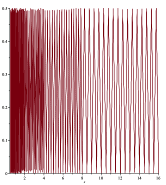
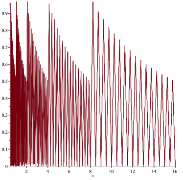
Figure 1: Left: absolute error (in ulps) of rounding to nearest $x\in[\frac{1}{2},16]$. Right: relative error (in multiples of $u=2^{-p}$) of rounding to nearest $x\in[\frac{1}{2},16]$. Both pictures assume a binary floating-point system with $p=5$.

It is obvious that Eq. 4 $\Rightarrow$ Eq. 5, but the reverse is not true. Still, although it conveys less information than Eq. 4, Eq. 5 is used more often than Eq. 4 in both paper-and-pencil and automated error analysis, because it is easier to manipulate relative errors when analyzing long sequences of operations. However, it is unlikely that near-optimal error bounds can be obtained using only Eq. 5, except for very short and simple algorithms. Figure 1 shows the absolute and relative errors resulting from rounding a real number $t\in[1/2,16]$. The absolute error bound $0.5\textnormal{ulp}$ is approached in the immediate vicinity of all real numbers, while the relative error bound $u$ is approached only slightly above powers of $2$. As a consequence, obtaining a near-optimal bound using Eq. 5 solely requires the existence of input values for which almost all intermediate variables in the computation under consideration are slightly above a power of $2$. While this may happen for very simple algorithms such as Algorithm 1 below, it is unlikely to happen for more complex algorithms.

1.3 Which kind of error bounds?

Generic and analytic bounds

Our aim is to determine relative error bounds that we term as generic and analytic for algorithms that typically contain at most a dozen or so arithmetic operations. We use these terms to denote that the bounds are expressed as a continuous function of $u$ that bounds the error for all $u$ that are less than some specified ${u_{\mathrm{max}}}>0$. To be more specific, we are interested in obtaining generic quadratic bounds, i.e., generic analytic bounds of the form

$$\alpha u+\beta u^{2},\qquad u\leq{u_{\mathrm{max}}}.$$ (6)

We look for “best possible” generic quadratic bounds: for $u\leq{u_{\mathrm{max}}}$ we want to minimize $\alpha$, and whenever possible, for that best $\alpha$ we want to minimize $\beta$. In particular, we do not want to return approximate bounds, such as those of the form “$\alpha u+\mathcal{O}(u^{2})$” that are frequent in numerical analysis, because they do not allow to guarantee that the error will be less than some well-defined value. To accomplish this, as said above, utilizing solely the relative error model (5) will not always be adequate. Instead, we often need to use the absolute-error model (4), in conjunction with particular properties of the set of FP numbers such as Lemma 2.1 or Lemma 2.4 below.

Consider, for a given algorithm an (absolute or relative) error bound $\mathcal{B}(u)$ and the (most likely unknown) worst case error $\mathcal{W}(u)$. We call the bound $\mathcal{B}$

• asymptotically optimal if $\mathcal{W}(u)/\mathcal{B}(u)\to 1$ as $u\to 0$;

• sharp (for $u\leq{u_{\mathrm{max}}}$) if $\mathcal{W}(u)\geq 0.999\mathcal{B}(u)$ for some values of $p$.

The exact motivation for a careful error analysis and the underlying hypotheses it uses may vary greatly from author to author, and this can influence the type of bound one looks for. As regards motivation for computing numerical error bounds, one can cite:

• Choosing between different algorithms: if two different algorithms are available to solve the same problem, one may wish to make an informed choice of the algorithm that has the best balance performance/accuracy. This requires that the error bounds be sharp (but approximate bounds could do).

• Careful implementation optimization: There is a comprehensive range of FP formats, ranging from $16$-bit “half-precision” formats to the $128$-bit “quad-precision” binary128 format. Since numbers represented in the small formats are processed faster, there is a temptation to use the small formats whenever possible [1]. As the small formats have significantly larger individual rounding errors, this requires sharp error bounds.

• Certainty: floating-point arithmetic is also used in critical numerical software (e.g., software embedded in transportation systems). For critical applications, it is sometimes essential to be sure that the numerical error does not exceed a certain limit. In such cases, the sharpness of the error bounds is not always needed, but certainty is paramount: approximate bounds are to be avoided.

Genericity versus optimality

The genericity of the error bounds avoids having to repeat the analysis for all possible FP formats. However, looking for generic bounds may mean giving up on optimality. The “best possible” generic analytic bound will sometimes not be sharp, because rounding errors are inherently “arithmetic”: they may depend on specific bit patterns in the binary representations of intermediate variables, which may be present only for some values of $p$. Consider for example the computation of $x^{2}-2$ using a multiplication followed by a subtraction, i.e., what is actually computed is $\textnormal{RN}(\textnormal{RN}(x^{2})-2)).$ Under the (generally accepted) conjecture [6] that $\sqrt{2}$ is a $2$-normal number (which implies than any given bit string appears infinitely many times in its binary representation), the behaviour of the algorithm is very different for $x=\textnormal{RN}(\sqrt{2})$ and the other values. The following properties hold:

• in precision-$p$ arithmetic, if $x\neq\textnormal{RN}(\sqrt{2})$ then the relative error of the computation is less than or equal to $\sqrt{2}/2\approx 0.707$;

• for infinitely many values of $p$, the largest relative error of the computation (hence attained for $x=\textnormal{RN}(\sqrt{2})$) is 1. This is found by choosing $p$ such that just after the first $p$ bits of the binary expansion of $\sqrt{2}$ there is either the bit-string $000$ or the bit string $111$ (the normality conjecture implies that there are infinitely many such $p$). In such cases, for $x=\textnormal{RN}(\sqrt{2})$, $\textnormal{RN}(x^{2})=2$ so that the computed result is zero;

• for infinitely many values of $p$, the relative error of the computation for $x=\textnormal{RN}(\sqrt{2})$ is less than $128/(112\sqrt{2}-49u)$, which is less than $0.876$ as soon as $u\leq 1/4$ (i.e., $p\geq 2$). This is found by choosing $p$ such that just after the first $p$ bits of the binary expansion of $\sqrt{2}$ there is either the bit-string $10000$ or the bit string $01111$.

Let $\mathcal{B}(u)$ be a generic analytic bound. (P2) implies that there are values of $u$ arbitrarily close to $0$ for which the largest error is $1$. For these values we must have $\mathcal{B}(u)\geq 1$ and since $\mathcal{B}$ is continuous by hypothesis, $\mathcal{B}(0)\geq 1$ so that for any $\epsilon>0$ there exists $u_{0}>0$ such that for $u<u_{0}$, we have $\mathcal{B}(u)\geq 1-\epsilon$. But (P1) and (P3) imply that there are infinitely many values of $p$ for which the largest relative error is less than $0.876$, implying that $\mathcal{B}(u)$ is not asymptotically optimal (and not even sharp).

1.4 Recent results

Recent results in computer arithmetic

Rump revisited the classical error bounds for recursive summation and dot product [40], showing that the usual “$\mathcal{O}(u^{2})$” terms which appear in the literature are not necessary. This prowess led to similar improvements for other problems such as summation in arbitrary order, polynomial evaluation, powers and iterated products, LU factorization, etc [41]. In this vein, Jeannerod and Rump proved optimal bounds for square-root and division [27], recalled in Lemma 2.4 below. These bounds offer precise control over the accuracy of fundamental operations. They are obtained through a delicate analysis of the discrete structure of the set of the FP numbers, which we do not attempt to automate here.

Recent work on automatic analysis

Various tools have been proposed for computing error bounds on the result of numerical programs. Noteworthy tools include Fluctuat [21] (based on abstract interpretation), FPTaylor and SATIRE [42, 17] (based on Taylor forms), Gappa [18] (based on interval arithmetic and forward error analysis), VCFloat2 [4] (based on interval arithmetic and a Coq tactic that recursively decomposes expressions), and Real2Float [34] (based on semidefinite programming and the use of (5)). They are very efficient in their respective domains (for instance Fluctuat and SATIRE can address rather large programs, Gappa and Real2Float can generate formal proofs or formally provable certificates, thence giving very good confidence on the obtained results). In general, they are somehow limited to a given precision (e.g., double-precision) and cannot return a bound of the form (6) valid with any $u\leq{u_{\mathrm{max}}}$. Moreover, the ability of handling large programs comes at the expense of bounds that may significantly exceed the optimal ones.

1.5 Contribution

Our approach is complementary to the works mentioned above. We provide generic analytic bounds parameterized by the unit round-off $u$. They are computed in such a way that some of the correlations between the errors in the intermediate steps are taken into account. This often yields tighter bounds than those provided by previous tools, at the expense of heavy computations. This limits our approach to the small programs that implement functions considered as “basic building blocks” of numerical computation, such as the hypotenuse considered in this article, for which it makes sense to spend much computing time in order to derive a sharp bound that will be reused many times, in many applications.

Running example: the hypotenuse function

We illustrate our approach with a gallery of algorithms for the computation of $\sqrt{x^{2}+y^{2}}$, presented in Section 4. A basic example is provided by the following naive program:

sx = x*x;
sy = y*y;
sigma = sx + sy;
rho1 = sqrt(sigma);

Assuming that the compiler does not change the sequence of instructions of the program, and that the arithmetic operations and the square root are rounded to nearest, what is actually computed is expressed by Algorithm 1 below.

Algorithm 1 The naive algorithm for the Hypot function. It takes $4$ FP operations, and approximates $\sqrt{x^{2}+y^{2}}$ with relative error better than $2u$.

1:  $s_{x}\leftarrow\textnormal{RN}(x^{2})$

2:  $s_{y}\leftarrow\textnormal{RN}(y^{2})$

3:  $\sigma\leftarrow\textnormal{RN}(s_{x}+s_{y})$

4:  $\rho\leftarrow\textnormal{RN}(\sqrt{\sigma})$

Assuming no underflow or overflow occurs, and just using Eq. 5 on each statement yields the relative error bound $2u+u^{2}$. This is the classical $2u+\mathcal{O}(u^{2})$ error bound of the literature [24]. Jeannerod and Rump improved that bound by showing that the relative error is actually less than $2u$ [27]. Both bounds are asymptotically optimal [26]. As a first example of our approach, we show in Section 5 that the error is bounded by

$$2u-\frac{8}{5}(9-4\sqrt{6})u^{2}<2u-\frac{5}{4}u^{2},\qquad u\leq 1/4.$$ (7)

Main tool: Polynomial Optimization

By the very nature of the FP numbers, the error is a discontinuous function of $u$ (and $u=2^{-p}$ itself only takes discrete values). However, the sharp error bounds that are known for the basic operations are all continuous functions of $u$ and, even better from the computer algebra point of view, algebraic functions (being obtained by combinations of $+,\times,\div,\sqrt{}$). Thus an algorithm can be seen as the description of a semi-algebraic set: a subset of $\mathbb{R}^{n}$ defined by polynomial equalities and inequalities. In the specific example of Algorithm 1, the equations are

$$\begin{split}s_{x}&=x^{2}(1+u\epsilon_{s_{x}}),\quad s_{y}=y^{2}(1+u\epsilon_{s_{y}}),\\ \sigma&=(s_{x}+s_{y})(1+u\epsilon_{\sigma}),\quad\alpha^{2}=\sigma,\quad\rho=\alpha(1+u\epsilon_{\rho}),\end{split}$$ (8)

with each $\epsilon_{i}$ bounded in absolute value by $1/(1+u)$. In general, tight bounds on these quantities $\epsilon_{i}$ are obtained by a step-by-step analysis of the program: in some cases they follow from a refinement of the relative error bound Eq. 5; in other cases knowledge of an interval containing the value allows the use of the tighter absolute error bound Eq. 4. In our example, this system of equalities and inequalities defines a small tube-like region of dimension 7 in $\mathbb{R}^{12}$: here, the dimension 12 comes from one variable for the unit round-off $u$, one for each input $x,y$, one for each of the variables of the algorithm ($s_{x},s_{y},\sigma,\rho$), one for each $\epsilon_{i}$ and one for the square-root $\alpha$. A computation reveals that the projection of this region on the $(u,x,y,\rho)$-coordinate space is simply the region between the surfaces $\rho=\sqrt{x^{2}+y^{2}}/(1+u)^{2}$ and $\rho=\sqrt{x^{2}+y^{2}}(1+2u)^{2}/(1+u)^{2}$. From there, it is easy to deduce the bound in Eq. 7.

For less straightforward algorithms, obtaining a bound becomes an optimization problem: find the maximum and the minimum of $\rho/\sqrt{x^{2}+y^{2}}-1$ in the domain defined by the equations and inequalities obtained from analyzing the program. This is an instance of the polynomial optimization problem, which consists in computing the maximum or the minimum of a variable that satisfies a given system of polynomial equations and inequalities. At this level of generality, this problem is well understood in terms of algorithms and complexity, see e.g., [37, 28, 7], but also very expensive. For large algorithms, one has no choice but to compute approximations to the optimal values; this is the approach taken by Real2Float [34]. We focus here on testing the limits of what can be computed exactly. Our approach exploits the specific structure of the problem as much as we can and is described in Section 3.

Prototype Implementation

We have written a simple Maple implementation of the approach described in this article. On the example above, its behaviour is as follows:

> Algo1:=[Input(x=0..2^16,y=0..2^16,_u=0..1/4),> s[x]=RN(x^2),s[y]=RN(y^2),sigma=RN(s[x]+s[y]),rho=RN(sqrt(sigma))]:> BoundRoundingError(Algo1);

$${\color[rgb]{0,0,1}2\textit{\_u}+\left(\frac{72}{5}-\frac{32\sqrt{6}}{5}\right)\textit{\_u}^{2}}$$

The algorithm is first stated with ranges for its inputs (currently the program only handles finite ranges, which is not much of a problem for the hypotenuse function, but might make the analysis somehow difficult for other functions). The name _u is used for the unit round-off. The procedure first makes several decisions concerning intermediate rounding errors; next, it computes a bound on the linear part of the error bound. Finally, the procedure computes an upper bound on the quadratic part once this linear part is fixed. This is the bound from Eq. 7. Thus in a way the input of our code is an algorithm and its output is a theorem giving an upper bound on its relative error. However, as mentioned above, since this is only a prototype, in this article we do not trust the output blindly. Instead, we use it as a statement of a theorem and give a paper proof, obtained mostly from following the intermediate steps of the code, so that the proof can be checked by a human reader.

1.6 Structure of the article

In Section 2, we recall special cases where the bounds Eq. 4 and Eq. 5 on the errors of individual operations can be improved due to some structural properties of the set of the FP numbers. Then, Section 3 describes the computer algebra algorithms we use for analyzing numerical programs. Section 4 presents several algorithms that have been proposed in the literature for evaluating the hypotenuse function. These algorithms are analyzed in Sections 5 to 9. We discuss these results in Section 10. The most technical parts of the analyses are deferred to Appendices A to C.

Acknowledgements

This work is partly supported by the ANR-NuSCAP 20-CE-48-0014 project of the French Agence nationale de la recherche (ANR). We are grateful to Mohab Safey El Din for giving us access to recent versions of his software, to Guillaume Melquiond for his help with Gappa and to Ganesh Gopalakrishnan and Tanmay Tirpankar for their help with Satire.

2 Bounds for Floating-Point Operations

Some structural properties of the set of FP numbers cannot be disregarded if tight error bounds are desired. An illustration is given by Lemma 2.1 below: if two FP numbers $a$ and $b$ are close enough, then computing $a-b$ results in no error. In such a case, utilizing Eq. 4 or Eq. 5 to bound the error would be a significant overestimation. A simpler example is multiplications by powers of two, which are exact operations as long as underflow and overflow are avoided.

Lemma 2.1 (Sterbenz’ Lemma [43]).

If $a$ and $b$ are floating-point numbers satisfying $a/2\leq b\leq 2a$ then $b-a$ is a floating-point number, which implies $\textnormal{RN}(b-a)=b-a$.

In a similar spirit, the following result of Boldo and Daumas [10, Thm. 5] is helpful to deal with the error in a square-root computation.

Lemma 2.2 (Exact representation of the square root remainder [10]).

In binary, precision-$p$, FP arithmetic with minimum exponent ${e_{\mathrm{min}}}$, let $s=\textnormal{RN}(\sqrt{t})$, where $t$ is a FP number. The term $t-s^{2}$ is a FP number if and only if there exists a pair of integers $(m,e)$ (with $|m|\leq 2^{p}-1$) such that $s=m\cdot 2^{e-p+1}$ and $2e\geq{e_{\mathrm{min}}}+p-1$.

An almost immediate consequence of Eq. 3 is the following slight improvement of Eq. 5.

Lemma 2.3 (Dekker-Knuth’s bound [32]).

If $t\neq 0$ is a real number in the normal domain, then the relative error due to rounding satisfies

$$\left|\frac{t-\textnormal{RN}(t)}{t}\right|\leq v\qquad\text{with}\quad v=\frac{u}{1+u}.$$ (9)

This bound was obtained by Dekker in 1971 [19] for the error of some operations in binary FP arithmetic. It was given by Knuth in its full generality [32]. But it is seldom used: most authors use the very slightly looser (but simpler) bound (5). In our context where the analyses are performed by a computer, we use Eq. 9 when appropriate.

Relative error for specific operations

Jeannerod and Rump [27] have showed that while the bound (9) is optimal for addition, subtraction and multiplication, it can be improved for division and square root. For these two operations, they give the following optimal bounds, of which we make heavy use.

Lemma 2.4 (Jeannerod-Rump bounds [27]).

When the precision $p$ is at least 2, the relative error of a (correctly rounded) square root is bounded by

$$1-\frac{1}{\sqrt{1+2u}};$$ (10)

the relative error of a division in binary FP arithmetic is bounded by

$$u-2u^{2}.$$ (11)

The first bound is general; the second one holds only in base 2, which is our setting in this article.

3 Computer algebra algorithms for tight analysis of numerical programs

We focus here on the analysis of straight-line programs operating over floating-point numbers. We assume that the basic operations in these programs are $+$, $-$, $\times$, $\div$, $\sqrt{.}$ and the FMA operation (which evaluates an expression $ab+c$ with one final rounding only and is available on all recent processors). Hence, such a program is a sequence of instructions, the $i$th one of which has one of the forms

$$v_{i}:=w_{j}\times w_{k}+w_{\ell}\quad\text{or}\quad v_{i}:=w_{j}\div w_{k}\quad\text{or}\quad v_{i}:=\sqrt{w_{j}},$$ (12)

where $w_{j},w_{k},w_{\ell}$ are either variables $v_{m}$ with $m<i$, or input variables, or constant floating-point numbers. For the first of the three forms (which corresponds to the FMA operation), taking some of the variables to be 0 or 1 recovers addition and multiplication. By convention, the last instruction defines the result of the algorithm, whose relative error is to be bounded. The analysis proceeds in three steps: a step-by-step analysis of the instructions of the program; an asymptotic analysis of an upper bound on the relative error as the precision tends to infinity (or equivalently, as $u$ tends to zero); an actual bound on the quadratic term in the relative error when using the asymptotic bound found for its linear part. We now review these steps in more detail.

3.1 Step-by-step analysis

This is the step where knowledge of the FP numbers from Sections 1.2 and 2 is used. It consists of an inductive construction of a system of polynomial equations and a system of inequalities.

First, a system $I_{0}$ of linear inequalities is initialized with the known information on the ranges of the input variables, plus the inequalities $0<u\leq u_{\max}$ for the unit round-off (see Section 2). The initial system of polynomial equations is the empty set: $S_{0}=\emptyset$.

The analysis proceeds instruction by instruction, constructing new systems of equations and inequalities $S_{i}$ and $I_{i}$ from $S_{i-1}$ and $I_{i-1}$. Let $t_{i}$ be the right-hand side of the assignment in the $i$th instruction of the algorithm from Eq. 12. This step aims at bounding the rounding error in the assignment $v_{i}:=t_{i}$ by analyzing $t_{i}$ using the systems $S_{i-1}$ and $I_{i-1}$.

No error

The best situation is when that error can be determined to be 0. This happens either when $t_{i}$ is a constant floating-point number that does not depend on the input variables, when a multiplication by a power of $2$ is performed, or when Sterbenz’ Lemma 2.1 or Lemma 2.2 are found to apply. As we construct only polynomial equations, the system $S_{i}$ is then obtained by adding one of the following to $S_{i-1}$:

$$v_{i}=w_{j}\times w_{k}+w_{\ell}\quad\text{or}\quad v_{i}w_{k}=w_{j}\quad\text{or}\quad v_{i}^{2}=w_{j}.$$ (13)

In the last case, we also add $v_{i}\geq 0$ to $I_{i-1}$ to obtain $I_{i}$. Otherwise, $I_{i}=I_{i-1}$.

Absolute error

The next best situation is when one can determine $\operatorname{ulp}(t_{i})$ exactly. For this, one determines the minimal and maximal values of $t_{i}$ given the equations and inequalities in $S_{i-1}$ and $I_{i-1}$. If these bounds allow to determine $\ell_{i}=\lfloor\log_{2}|t_{i}|\rfloor$ exactly, then the system is enriched with an absolute error bound: in Eq. 13, $v_{i}$ is replaced by

$$v_{i}+2^{\ell_{i}+1}\epsilon_{i}u,$$ (14)

and the system of inequalities is complemented with $-1\leq\epsilon_{i}\leq 1$.

Relative error

In the remaining cases, the systems are enriched with a relative error bound:

$$v_{i} =(w_{j}\times w_{k}+w_{\ell})(1+\epsilon_{i}u), -b_{DK} \leq\epsilon_{i}\leq b_{DK}$$ (15)

or $$v_{i}w_{k} =w_{j}(1+\epsilon_{i}u), -b_{\div} \leq\epsilon_{i}\leq b_{\div},$$ (16)

or $$v_{i}^{2} ={w_{j}}(1+\epsilon_{i}u)^{2}, -b_{\sqrt{}} \leq\epsilon_{i}\leq b_{\sqrt{}},\quad v_{i}\geq 0,$$ (17)

and the relevant equation and inequality among

$$\begin{split}(1+u)b_{DK}=1,\quad b_{\div}=u-2u^{2},\qquad\\ u(1+2u)b_{\sqrt{}}^{2}-2(1+2u)b_{\sqrt{}}+2=0,\quad b_{\sqrt{}}\geq 0,\end{split}$$ (18)

that come from Lemmas 2.4 and 2.3.

3.2 Polynomial optimization

The end result of the step-by-step analysis is a system of polynomial equations and a system of polynomial inequalities, where each statement of the algorithm brings one equation in one or two new variables (two being the general case when the error is not zero) and a certain number of inequalities.

At each stage of the step-by-step analysis and when bounding the relative error on the last variable, we need to find the minimum or maximum of a quantity defined by the system. Without loss of generality and up to adding equations to the system, we can assume that the quantity to be maximized or minimized is the last variable $v_{m}$ introduced in the system.

As mentioned in the introduction, this problem is well-understood in terms of algorithms and complexity but also very expensive. In practice, even with efficient software such as Mohab Safey el Din’s Raglib library, which relies on Faugère’s FGb library for Gröbner bases, we could not obtain our bounds directly using general-purpose approaches, except for the simplest algorithms.

Instead, we take an approach that exploits two characteristics of our systems of polynomial equalities and inequalities:

1. As the unit round-off $u$ is typically small compared to the other variables of the program, the set of inequalities describes a small tube-like semi-algebraic set around the exact value the variables take at $u=0$;

2. Being produced by the step-by-step analysis described above, the set of polynomial equalities we start with has a triangular structure.

Free and dependent variables.

We distinguish two types of variables in these systems: the free variables are the variables $\epsilon_{i}$ encoding the absolute or relative errors, the input variables and the unit round-off $u$; the dependent variables are those whose value is fixed once the free ones are fixed. Initially, they correspond to the variables $v_{i}$ defined by the algorithm itself, as well as the bound variables from Eq. 18.

The optimization is a recursive process where at each step one equation is added to the system, making one of the free variables dependent and maintaining the triangular nature of the system. At the end, no free variables are left and the optimum is found among finitely many values. We now describe this process in more detail.

Gradient.

As the system $S_{m}$ obtained by the step-by-step analysis is triangular, by repeated use of the chain rule, the gradient of the last variable $u_{m}$ with respect to the free variables is obtained as a vector of rational functions in all variables. Equivalently, this can be computed by automatic differentiation.

Recursive optimization.

The optimization is a recursive search of extrema. It is performed by looping through the free variables and trying to detect whether the sign of the partial derivative with respect to one of them can be decided (see Section 3.3). If this is the case, a new equation is added to the system, setting this variable to its extremal value from Eq. 18 and one gets an expression in one variable less to be optimized. When the decision cannot be reached for any of the free variables, then we pick one of the variables $\epsilon_{i}$ (heuristic choices are made) and use a branch-and-bound method, optimizing the polynomial in each of the three cases $\partial u_{m}/\partial\epsilon_{i}=0$ or $\epsilon_{i}$ equal to its extremal values. The new systems have one variable less.

3.3 Sign decisions

Being able to quickly decide the sign of a polynomial in the domain of optimization gives a substantial speed-up in the computation by removing many branches in the optimization tree. This is where we use the fact that several of the variables live in a small domain. Several techniques are used to help this decision.

Factorization

of multivariate polynomials over the rationals is well understood in theory [31, 44] and works well in practice. It is not needed by the algorithms but allows to reduce the degrees and possibly the number of variables of the polynomials whose signs have to be decided.

Interval arithmetic

can be applied since for each variable, be it free or dependent, we have bounds at our disposal that have been computed during the step-by-step analysis. In some cases, this is sufficient to decide the sign.

Small number of variables

occur near the bottom of the recursion tree. A classical way to decide that a polynomial in one variable does not vanish inside a given interval is to use Sturm sequences. These are available in all major computer algebra systems.

For a univariate algebraic expression $A(x)$, e.g., a combination of $+,\times,\div,\sqrt{}$ applied to constants and one variable $x$, it is easy to construct by induction a nonzero bivariate polynomial $Q(x,y)$ such that $Q(x,A(x))=0$. Then a sufficient condition for $A$ not to vanish in a given interval is that the constant term $Q(x,0)$ does not vanish there. This reduces the problem to that of a polynomial in one variable. While this is only a sufficient condition, this method saves a significant amount of time when it applies.

3.4 Regular chains

We take advantage of the triangular shape of the system constructed by the step-by-step analysis of Section 3.1 using regular chains. These were studied initially by Lazard [33] and Kalkbrener [30] and a large number of efficient algorithms have been developed since [5, 14, 15, 16, 13, 3].

We first recall the basic notions. The polynomials belong to $\mathbb{K}[x_{1},\dots,x_{n}]$ for an algebraically closed field $\mathbb{K}$. $\mathbb{K}$ can be the field $\mathbb{C}$ of complex numbers, but usually, the coefficients of the polynomials are rational functions in the free variables with rational coefficients, while the variables $x_{i}$ are the dependent variables. An order $x_{n}>\dots>x_{1}$ is fixed on the variables. The leading variable of a polynomial is the largest variable on which it depends. A set $T$ of polynomials is triangular when the polynomials have pairwise distinct leading variables.

The coefficient of highest degree of a polynomial with respect to its leading variable is called the initial of the polynomial. The product of the initials of a triangular set $T$ is denoted $h_{T}$. Three geometric notions are relevant: the zero set $V(T)\subset\mathbb{K}^{n}$ of zeros of $T$; the quasi-component $W(T)=V(T)\setminus V(h_{T})$ and its Zariski closure $\overline{W(T)}$.

Regular chains are defined inductively. An empty triangular set $T$ is a regular chain. Otherwise, if $T_{\max{}}$ is the element of a triangular set $T$ with the largest leading variable, $T$ is a regular chain when $T^{\prime}:=T\setminus\{T_{\max{}}\}$ is a regular chain and the the initial $h_{\max}$ of the polynomial $T_{\max{}}$ is regular in the sense that $\overline{W(T^{\prime})}=\overline{W(T^{\prime})\setminus V(h_{\max})}$.

The following example illustrates all these notions.

Example 3.1.

Consider a program that would perform the sequence of assignments

$$t_{2}:=\sqrt{2}t_{1},\quad t_{3}:=t_{1}^{2}/t_{2}.$$ (19)

For the second assignment not to raise an error, it is necessary that $t_{2}\neq 0$. The computed values are such that the point $(t_{1},t_{2},t_{3})$ is part of the solution set of the polynomial system

$$T=\{t_{2}^{2}-2t_{1}^{2},t_{3}t_{2}-t_{1}^{2}\}.$$

This is a regular chain for the order $t_{3}>t_{2}>t_{1}$. Its solution set is the union of two curves: $V(T)=\mathcal{C}_{1}\cup\mathcal{C}_{2}$, with

$$\mathcal{C}_{1}=\{(\pm\sqrt{2}t,2t,t)\mid t\in\mathbb{C}\},\qquad\mathcal{C}_{2}=\{(0,0,t)\mid t\in\mathbb{C}\}.$$

The product of initials in $T$ is $h_{T}=t_{2}$ and thus the quasi-component is just the first curve minus a point: $W(T)=\mathcal{C}_{1}\setminus\{(0,0,0)\}$. All values computed by Eq. 19 belong to $W(T)$. Finally, the Zariski closure recovers the missing point and $\overline{W(T)}=\mathcal{C}_{1}$.

3.5 Application to Error Analysis

The systems of equations constructed during the step-by-step analysis of Section 3.1 are actually regular chains. The field one starts with is the field of rational functions $\mathbb{K}_{0}:=\mathbb{Q}(u,i_{1},\dots,i_{\ell})$ in $u$ the unit round-off and $i_{1},\dots,i_{\ell}$ the input variables.

Starting from $I_{i-1}$ a regular chain in $\overline{\mathbb{K}_{i-1}}[v_{1},\dots,v_{i-1}]$ for the order $v_{1}<\dots<v_{i-1}$, the chain is enriched by the relevant equation from Eq. 13, Eq. 14 or Eqs. 15, 16 and 17, while the field $\mathbb{K}_{i}$ is $\mathbb{K}_{i-1}$ when it is detected that no error occurs and $\mathbb{K}_{i-1}(\epsilon_{i})$ otherwise. The new variable $v_{i}$ is set to be larger than $v_{i-1}$ in the ordering; the main variable of the new polynomial is thus $v_{i}$, so that the system is triangular; its initial is 1, except in the case of a division where it is $w_{k}$. In that situation, removing $V(w_{k})$ is expected, as it corresponds to a division by 0. Thus, computing quasi-components is desired in our setting.

The construction of the regular chains used during the optimization is different. This occurs during the step-by-step analysis to determine the extremal values of the variables or during the computation of relative error bounds. During such an optimization, new equations involve free variables that become dependent and are removed from the current field of coefficients. These new dependent variables are appended to the list of dependent variables in descending order: if, before the optimization, the system defines the variables $v_{m}>v_{m-1}>\dots>v_{1}$, during the optimization the variables are given by a regular chain $T$ that also defines $f_{1}>\dots>f_{k-1}$ with the $f_{i}$ formerly free variables and $v_{1}>f_{1}$.

The introduction of a new variable $f_{k}$ is through a polynomial $p(f_{k})$. The equation $p(f_{k})=0$ indicates that a derivative is 0, or that one of the $\epsilon_{i}$, one of the input variables, or the unit round-off $u$ is assigned one of its possible extremal values. A new field $\tilde{\mathbb{K}}$ is defined with one variable less so that the previous one is $\tilde{\mathbb{K}}(f_{k})$. At this stage, the current regular chain $T$ is 1-dimensional over the current field, as all dependent variables except $f_{k}$ are given by a polynomial in the chain. An important issue is that it is not sufficient to consider the intersection $W(T)\cap V(p(f_{k}))$, for which many algorithms are available, but we need to know the closure $\overline{W(T)}\cap V(p(f_{k}))$. As an illustration of the difference, if the current system is

$$T=[2t_{3}t_{1}^{2}-2(t_{1}+1)t_{2}-2t_{1}^{2}+3t_{1}+2,t_{2}^{2}-t_{1}-1]$$

with $t_{3}>t_{2}>t_{1}$, then the intersection $W(T)\cap V(t_{1})$ is empty, whereas $\overline{W(T)}\cap V(t_{1})=\{(0,1,11/8)\}$. The fact that our construction always involves 1-dimensional regular chains lets us compute these closures thanks to an algorithm by Alvandi et al. [3], implemented in the function LimitPoints of the Maple package RegularChains[AlgebraicGeometryTools].

4 A gallery of algorithms for the hypotenuse

Our running example is the calculation of the hypotenuse function $(x,y)\mapsto\sqrt{x^{2}+y^{2}}$. We now present various algorithms for that function that we use to illustrate our approach, each with its own motivation and merits. The naive algorithm (Algorithm 1) is simple, fast, and fairly accurate: when no underflow/overflow occurs, the absolute error is bounded by $1.222~{}\textnormal{ulp}$, as shown by Ziv [46], and the relative error is bounded by $2u$. However, Algorithm 1 suffers from a serious drawback: intermediate calculations can underflow or overflow, even if $\sqrt{x^{2}+y^{2}}$ is far from the underflow or overflow thresholds. Such spurious underflows or overflows can result in infinite or very inaccurate output. For instance, assuming we use the binary64 (a.k.a. “double precision”) format of the IEEE 754 Standard,

• if $x=2^{600}$ and $y=0$ the returned result is $+\infty$ (because the computation of $x^{2}$ overflows) whereas the exact result is $2^{600}$;

• if $x=65\times 2^{-542}$ and $y=72\times 2^{-542}$ the returned result is $96\times 2^{-542}$ whereas the exact result is $97\times 2^{-542}$.

The usual solution to overcome this problem is to scale the input data, i.e., to multiply or divide $x$ and $y$ by a common factor such that overflow becomes impossible and underflow becomes either impossible or harmless. This is for instance what Algorithm 2 below does, in a rather straightforward way.

To counter spurious overflow, one can divide both operands by the one with the largest magnitude. This gives the well-known Algorithm 2, which is used for example in Julia 1.1. Spurious underflow is not completely avoided, but if one of the input variables (say, $y$) is so small in magnitude before the other one that $|y/x|$ is below the underflow threshold, then $\sqrt{x^{2}+y^{2}}$ is approximated by $|x|$ with very good accuracy, so that the result returned by the algorithm is excellent. Unfortunately, as we are going to see, Algorithm 2 is significantly less accurate than Algorithm 1.

Algorithm 2 The simplest scaling for the Hypot function: divide both operands by the one with the largest magnitude.

1:  if $|x|<|y|$ then

2:     swap$(x,y)$

3:  end if

4:  $r\leftarrow\textnormal{RN}(y/x)$

5:  $t\leftarrow\textnormal{RN}(1+r^{2})$

6:  $s\leftarrow\textnormal{RN}(\sqrt{t})$

7:  $\rho_{2}=\textnormal{RN}(|x|\cdot s)$

Beebe [8] suggests several solutions to compensate for the loss of accuracy in Algorithm 2 (using an adaptation of the Newton-Raphson iteration for the square root). One of them is Algorithm 3 below, whose first $6$ lines are exactly the same as those of Algorithm 2. As shown in Section 7, it does more than just compensate for the loss of accuracy due to the scaling: it has a better final error bound than Algorithm 1.

Algorithm 3 Improvement of Algorithm 2 suggested by Beebe [8].

1:  if $|x|<|y|$ then

2:     swap$(x,y)$

3:  end if

4:  $r\leftarrow\textnormal{RN}(y/x)$

5:  $t\leftarrow\textnormal{RN}(1+r^{2})$

6:  $s\leftarrow\textnormal{RN}(\sqrt{t})$

7:  $\epsilon\leftarrow\textnormal{RN}(t-s^{2})$

8:  $c\leftarrow\textnormal{RN}(\epsilon/(2s))$

9:  $\nu\leftarrow\textnormal{RN}(|x|\cdot c)$

10:  $\rho_{3}\leftarrow\textnormal{RN}(|x|\cdot s+\nu)$

Borges [12] presents several algorithms, including the very accurate Algorithm 4 below. It does not address the spurious under/overflow problem (one has to assume that a preliminary scaling by a power of $2$ has been done). The Fast2Sum and Fast2Mult algorithms called by Algorithm 4 are well-known building blocks of computer arithmetic (see for instance [11]). Here we just need to know that Fast2Mult$(x,y)$ (resp. Fast2Sum$(x,y)$) delivers a pair $(a,b)$ of FP numbers such that $a=\textnormal{RN}(xy)$ (resp. $a=\textnormal{RN}(x+y)$) and $b=xy-a$ (resp. $b=(x+y)-a$). As shown in Section 8, this algorithm is almost optimal in terms of relative error (we obtain a relative error bound slightly above $u$).

Algorithm 4 Borges’ corrected “fused” algorithm [12, Algorithm 5].

1:  if $|x|<|y|$ then

2:     swap$(x,y)$

3:  end if

4:  $(s_{x}^{h},s_{x}^{\ell})\leftarrow$ Fast2Mult$(x,x)$

5:  $(s_{y}^{h},s_{y}^{\ell})\leftarrow$ Fast2Mult$(y,y)$

6:  $(\sigma_{h},\sigma_{\ell})\leftarrow$ Fast2Sum$(s_{x}^{h},s_{y}^{h})$

7:  $s\leftarrow\textnormal{RN}\left(\sqrt{\sigma_{h}}\right)$

8:  $\delta_{s}\leftarrow\textnormal{RN}(\sigma_{h}-s^{2})$

9:  $\tau_{1}\leftarrow\textnormal{RN}(s_{x}^{\ell}+s_{y}^{\ell})$

10:  $\tau_{2}\leftarrow\textnormal{RN}(\delta_{s}+\sigma_{\ell})$

11:  $\tau\leftarrow\textnormal{RN}(\tau_{1}+\tau_{2})$

12:  $c\leftarrow\textnormal{RN}(\tau/s)$

13:  $\rho_{4}\leftarrow\textnormal{RN}(c/2+s)$

Kahan [29] gives the fairly accurate Algorithm 5 below. It avoids spurious underflows and overflows. Although we do not discuss these matters here, it also has the advantage of correctly setting the various IEEE 754 exception flags (underflow, overflow, inexact). It has the kind of size where automation of the analysis becomes a necessity if one is not satisfied with loose error bounds.

Algorithm 5 Kahan’s hypot Algorithm [29, Algorithm CABS]. In this presentation, it requires the availability of an FMA instruction. We assume $0\leq y\leq x$. The algorithm uses the precomputed constants $R_{2}=\textnormal{RN}(\sqrt{2})$, $P_{h}=\textnormal{RN}(1+\sqrt{2})$, and $P_{\ell}=\textnormal{RN}(1+\sqrt{2}-P_{h})$.

1:  $\delta\leftarrow\textnormal{RN}(x-y)$

2:  if $\delta>y$ then

3:     $r\leftarrow\textnormal{RN}(x/y)$

4:     $t\leftarrow\textnormal{RN}(1+r^{2})$

5:     $s\leftarrow\textnormal{RN}(\sqrt{t})$

6:     $z\leftarrow\textnormal{RN}(r+s)$

7:  else

8:     $r_{2}\leftarrow\textnormal{RN}(\delta/y)$

9:     $tr_{2}\leftarrow\textnormal{RN}(2r_{2})$

10:     $r_{3}\leftarrow\textnormal{RN}(tr2+r_{2}^{2})$

11:     $r_{4}\leftarrow\textnormal{RN}(2+r_{3})$

12:     $s_{2}\leftarrow\textnormal{RN}(\sqrt{r_{4}})$

13:     $d=\textnormal{RN}(R_{2}+s_{2})$

14:     $q=\textnormal{RN}(r_{3}/d)$

15:     $r_{5}\leftarrow\textnormal{RN}(P_{\ell}+q)$

16:     $r_{6}\leftarrow\textnormal{RN}(r_{5}+r_{2})$

17:     $z\leftarrow\textnormal{RN}(P_{h}+r_{6})$

18:  end if

19:  $z_{2}\leftarrow\textnormal{RN}(y/z)$

20:  $\rho_{5}\leftarrow\textnormal{RN}(x+z_{2})$

These algorithms are sorted by order of complexity of their analysis. We now deal with them in order, introducing the new problems and solutions one at a time.

5 Algorithm 1: Straightforward Analysis

As mentioned in the introduction, the relative error of Algorithm 1 is bounded by $2u$ and that bound is asymptotically optimal. We now show how this result is derived by our approach, and how a small term $\frac{5}{4}u^{2}$ can be subtracted from the previous bound.

Step-by-step analysis

The result of a step-by-step analysis was given in Eq. 8. It follows that the relative error $\rho/\sqrt{x^{2}+y^{2}}-1$ equals

$$R=\frac{\sqrt{\left(x^{2}(1+u\epsilon_{s_{x}})+y^{2}(1+u\epsilon_{s_{y}})\right)(1+u\epsilon_{\sigma})}\,(1+u\epsilon_{\rho})}{\sqrt{x^{2}+y^{2}}}-1,$$

where each of $\epsilon_{s_{x}},\epsilon_{s_{y}},\epsilon_{\sigma}$ has absolute value bounded by $1/(1+u)$, by Eq. 9, while $\epsilon_{\rho}$ is bounded by the Jeannerod-Rump bound of Eq. 10. The next step of the analysis is to find the maximal value of $|R|$ when all the $\epsilon$ variables range in these intervals. Note that all these bounds are smaller than 1.

Upper bound

Since $0<u<1$, the expression above is an increasing function of each of these $\epsilon_{i}$ in their intervals. Therefore its minimum is reached when they are all simultaneously equal to their minimum, and similarly for the maximal value. When $\epsilon_{s_{x}}=\epsilon_{s_{y}}=\epsilon_{\sigma}$ with $\epsilon$ their common value, the expression of $R$ simplifies to

$$(1+u\epsilon)(1+u\epsilon_{\rho})-1=u(\epsilon+\epsilon_{\rho})+u^{2}\epsilon\epsilon_{\rho}.$$

This shows that the absolute value of the relative error $R$ is maximal when $\epsilon$ and $\epsilon_{\rho}$ both reach their maximal value, giving

$$|R|\leq S(u):=\frac{1+2u}{1+u}\left(2-\frac{1}{\sqrt{1+2u}}\right)-1=\frac{1+3u-\sqrt{1+2u}}{1+u}.$$

As $u\rightarrow 0$,

$$S(u)=2u-\frac{3}{2}u^{2}+u^{3}+O(u^{4}),$$

showing the linear term in the bound. If only the linear term $2u$ is needed, using the simple bound from Eq. 5 is sufficient. The more refined estimates are only required to control the difference between that linear term and the actual error.

Optimal quadratic term

Next, consider

$$y(u)=\frac{S(u)-2u}{u^{2}},$$

whose maximum for $u\in(0,u_{\max}]$ gives an upper bound on the quadratic term of the error bound. This function is $C^{\infty}$ for $u>-1/2$ and the Taylor expansion above shows that $y(0)=-3/2$ and $y^{\prime}(0)=1$. From the explicit expression of $S$, it is easy to see that $y^{\prime}>0$ in the interval $[0,1/4]$, implying that for $u_{\max}\leq 1/4$ its maximum — the bound we are after — is reached at $u_{\max}$. Thus we have proved the following.

Theorem 5.1.

Barring underflow and overflow, the relative error $R$ of Algorithm 1 for $u\leq 1/4$ satisfies

$$|R|\leq\frac{1+3u-\sqrt{1+2u}}{1+u}=2u+\kappa u^{2},\quad\kappa<-5/4.$$

The bound given in the introduction and obtained by our program for $u=1/4$ can be seen to be $y(1/4)$. The bound $y(1/4)<-5/4$ follows by numerical approximation. Other values of the quadratic bound are given in Table 1.

lower bound on $p$	upper bound on the error
8	$2u-\frac{3}{2}u^{2}+4\cdot 10^{-3}u^{2}$
11	$2u-\frac{3}{2}u^{2}+5\cdot 10^{-4}u^{2}$
24	$2u-\frac{3}{2}u^{2}+6\cdot 10^{-8}u^{2}$
53	$2u-\frac{3}{2}u^{2}+2\cdot 10^{-16}u^{2}$
113	$2u-\frac{3}{2}u^{2}+10^{-34}u^{2}$

Table 1: Quadratic error bound for Algorithm 1

Proof based on polynomials

In preparation for more complicated examples where the analysis of the function $S(y)$ is not as straightforward as here, we show how computer algebra could be used to show that $y^{\prime}>0$ in the interval $[0,1/4]$. The starting point is to perform a simple manipulation (automated in the Maple gfun package) showing that $y$ satisfies the quadratic equation

$$E(y,u)=u^{2}(1+u)^{2}y^{2}-2(1-u^{2})(1+2u)y+(1+2u)(2u-3)=0.$$

By continuity, $y^{\prime}$ is positive in a neighborhood of $u=0$. It can only change sign at a point $u$ where $y^{\prime}=0$, but then

$$\frac{\partial E}{\partial u}+\frac{\partial E}{\partial y}y^{\prime}=0$$

implies $\partial E/\partial u(y,u)=0$. Eliminating $y$ between $E=0$ and $\partial E/\partial u=0$ by means of a resultant shows that in turn, this implies

$$(1+u)(4+21u+32u^{2}+12u^{3}-8u^{4})=0.$$

Now, a simple interval analysis shows that this polynomial does not vanish for $u\in[0,1/2]$. Thus $y^{\prime}$ does not vanish in this interval and $y^{\prime}(0)>0$ shows that $y$ is an increasing function.

Then, a direct proof of the bound $-5/4$ consists in using continuity again, considering the univariate polynomial $E(-5/4,u)$ and observing its absence of root in $[0,1/2]$, which shows that $-5/4$ is never reached by $y(u)$ in this interval.

6 Algorithm 2: Exploit Absolute Errors

A direct analysis using only the simple relative error bound Eq. 5 leads to a bound on the relative error with a linear term of order $3u$. The refined estimates on the relative error from Section 2 do not improve that linear term. A step-by-step analysis of the program yields a better estimate by studying more carefully the ranges of the intermediate variables.

We assume $0\leq y\leq x$ (i.e., we consider that if needed, the swap of Line 2 of the algorithm has already been done).

6.1 Automatic Analysis

The result of our automation is as follows.

> Algo2:=[Input(x=0..2^16,alpha=0..1),y=RN(alpha*x,0),> r=RN(y/x),t=RN(1+r^2),s=RN(sqrt(t)),rho=RN(x*s)]:> BoundRoundingError(Algo2);

$${\color[rgb]{0,0,1}\frac{5}{2}\_u+\frac{3}{8}\_u^{2}}$$

The assumption $0\leq y\leq x$ is encoded by introducing a variable $\alpha\in[0,1]$ and stating that $y=\alpha x$ without an error, by using a second argument to RN that encodes special knowledge on the error for a specific operation.

6.2 Result

The output of our program is an indication pointing to the following result, proved below.

Theorem 6.1.

The relative error of Algorithm 2 is less than or equal to

$$R_{5}(u)=\frac{(1+2u)\sqrt{1+u}-1+2u^{2}}{1+u}\leq\frac{5}{2}u+\frac{3}{8}u^{2}.$$

Proposition 6.2.

The bound of Theorem 6.1 is asymptotically optimal.

Proof.

Choose $x=2^{p}-1$ and

$$y=\textnormal{RN}\left((2^{p}-1)\cdot\sqrt{7}\cdot 2^{-p/2}\cdot(1-u)^{2}\right).$$

As soon as $u\leq 1/32$, following the steps of the algorithm shows that its output is $\rho_{2}=2^{p}$. It follows that $\sqrt{x^{2}+y^{2}}-\rho_{2}\to\frac{5}{2}$ as $u\to 0$, so that the relative error is asymptotically equivalent to $5u/2$. ∎

The following example illustrates the sharpness of the bound: in the binary64 format, with

$$x=9007199254740991\quad\text{and}\quad y={8425463406411589}\times 2^{-25},$$

the relative error is $2.49999999999999558648u$.

We now detail the steps of the analysis leading to the proof of Theorem 6.1, following the approach outlined in Section 3.

6.3 Step-by-step analysis

This stage translates the program into a polynomial system with bounds on intermediate error-variables. The first two steps give the equalities

$$y=\alpha x,\quad rx=y(1+u\epsilon_{r}),$$

with $|\epsilon_{r}|\leq 1-2u$ by the Jeannerod-Rump bound Eq. 11.

Next, since $r$ is the rounded value of $\alpha\in[0,1]$ and the function RN is increasing, $r\leq\textnormal{RN}(1)=1$. This implies that $1\leq 1+r^{2}\leq 2$ and therefore also $1\leq\textnormal{RN}(1+r^{2})\leq 2$. Hence the rounding absolute error committed at Line 5 of Algorithm 2 is less than $u$ (half the distance between two consecutive FP numbers between $1$ and $2$). The same reasoning applies to $\sqrt{t}$. This gives

$$t=1+r^{2}+u\epsilon_{t},\quad s=\sqrt{t}+u\epsilon_{s},$$

with $|\epsilon_{s}|$ and $|\epsilon_{t}|$ bounded by $1$.

The last step is analyzed as before, giving

$$\rho=xs(1+u\epsilon_{\rho}),$$

with $|\epsilon_{\rho}|\leq 1/(1+u)$, by Eq. 9.

It follows from these equations that the relative error $|\rho/\sqrt{x^{2}+y^{2}}-1|$ is upper bounded by $|R|$, where

$$R=\frac{\left(\sqrt{1+\alpha^{2}(1+u\epsilon_{r})^{2}+u\epsilon_{t}}+u\epsilon_{s}\right)(1+u\epsilon_{\rho})}{\sqrt{1+\alpha^{2}}}-1.$$

6.4 Upper bound

As in the analysis of Section 5, for $u\leq 1/4$, since all the $|\epsilon_{i}|$ are bounded by 1, $R$ above is an increasing function of all the $\epsilon_{i}$ in their intervals. Writing

$$\epsilon_{r}=\epsilon(1-2u),\quad\epsilon_{s}=\epsilon,\quad\epsilon_{t}=\epsilon,\quad\epsilon_{\rho}=\frac{\epsilon}{1+u},$$

it follows that $R$ is bounded between the values taken by

$$\tilde{R}(\alpha,\epsilon):=\frac{\left(\sqrt{1+\alpha^{2}(1+\epsilon u(1-2u))^{2}+u\epsilon}+u\epsilon\right)\left(1+\epsilon\frac{u}{1+u}\right)}{\sqrt{1+\alpha^{2}}}-1$$

at $\epsilon=-1$ and at $\epsilon=1$. The variation of these bounds with respect to $\alpha$ is dictated by

$$\frac{\partial\tilde{R}}{\partial\alpha}=\left(1+\epsilon\frac{u}{1+u}\right)\frac{\alpha}{(1+\alpha^{2})^{3/2}}\\ \times\frac{(1+\epsilon u(1-2u))^{2}-1-u\epsilon-u\epsilon\sqrt{1+\alpha^{2}(1+\epsilon u(1-2u))^{2}+u\epsilon}}{\sqrt{1+\alpha^{2}(1+\epsilon u(1-2u))^{2}+u\epsilon}}.$$

With $u\leq 1/4$, $\epsilon\in\{-1,1\}$ and $\alpha\in[0,1]$, the signs of each of these factors can be analyzed directly. The first two are nonnegative, as is the denominator of the third one. Its numerator rewrites as

$$u\epsilon\left(1-(4-\epsilon)u-4\epsilon u^{2}(1-u)-\sqrt{1+\alpha^{2}(1+\epsilon u(1-2u))^{2}+u\epsilon}\right).$$

The first factor is positive, the second one has the sign of $\epsilon$ and the last one is negative. Indeed, the argument of the square root is increasing with $\epsilon$ and $\alpha$, so that its minimum is larger than $\sqrt{1-u}$, itself larger than $1-u$ for $u\in[0,1]$. Thus this last factor is upper bounded by

$$-1+u+1-(4-\epsilon)u-4\epsilon u^{2}(1-u)\leq-3u+\epsilon u-4\epsilon u^{2}(1-u)\\ \leq-2u+4u^{2}(1-u)\leq-u<0.$$

In conclusion, at $\epsilon=-1$, $\tilde{R}$ is negative and increasing with $\alpha$, while at $\epsilon=1$, it is positive and decreasing with $\alpha$. Thus in both cases, its absolute value is maximal at $\alpha=0$. Therefore $R$ is bounded between the values taken by

$$\tilde{R}(0,\epsilon):={\left(\sqrt{1+u\epsilon}+u\epsilon\right)\left(1+\epsilon\frac{u}{1+u}\right)}-1$$

at $\epsilon=-1$ and at $\epsilon=1$. It can now be observed that this is maximal in absolute value at $\epsilon=1$ so that we have obtained the upper bound of the theorem

$$|R|\leq S(u):=\frac{(1+2u)\sqrt{1+u}-1+2u^{2}}{1+u}.$$

As $u\rightarrow 0,$

$$S(u)=\frac{5}{2}u+\frac{3}{8}u^{2}-\frac{9}{16}u^{3}+O(u^{4}).$$

6.5 Optimal quadratic term

Set $y(u)=({S(u)-\frac{5}{2}u})/{u^{2}}$, which satisfies the quadratic equation

$$E(y,u)=4u^{2}(1+u)^{2}y^{2}+4(1+u)(u^{2}+5u+2)y+u^{2}-6u-3=0.$$

We now show that $y^{\prime}<0$ in the interval $[0,u_{\max}]$, implying that the maximum of $y$ is reached at $u=0$, where it is $3/8$, as can be seen from the Taylor expansion above.

By continuity, $y^{\prime}$ is negative in a neighborhood of $u=0$. The vanishing of $y^{\prime}$ can only occur at a zero of the resultant of $E$ and $\partial E/\partial u$, which implies

$$(1+u)^{3}(1+2u)^{2}(u^{3}-16u^{2}-22u-9)=0.$$

A simple analysis (e.g., by Sturm sequences) shows that this does not vanish for $u$ in $[0,1]$. This proves that $y^{\prime}<0$ in that region and concludes the proof of the theorem.

7 Algorithm 3: Split Argument Interval

In the analysis of Algorithm 3, a new technique is necessary in order to obtain an optimal linear bound: splitting the domain of the parameters into two subdomains. The location of the split follows from the analysis and is presented as a suggestion by the implementation.

As in the previous analysis, we assume that, if needed, the swap of Line 2 of the algorithm already took place, and we assume without loss of generality that the operands are positive, so that $0\leq y\leq x$. We also assume $p\geq 4$ (i.e., ${u_{\mathrm{max}}}=1/16$). Also, as in the previous algorithm, we set $\alpha={y}/{x}$ and discuss according to its value.

7.1 Automatic analyses

A first analysis is misleading:

> Algo3:=[Input(x=0..2^16,alpha=0..1),y=RN(alpha*x,0),> r=RN(y/x),t=RN(1+r^2),s=RN(sqrt(t)),> epsilon=RN(t-s^2,0),c = RN(epsilon/2/s),nu = RN(x*c),> rho=RN(nu+x*s)]:> BoundRoundingError(Algo3);

$$\color[rgb]{0,0,1}\frac{7}{4}\textit{\_u}+\left(\sqrt{2}-\frac{33}{32}\right)\textit{\_u}^{2}$$

Recall that the second argument 0 of the rounding function RN indicates that this operation is exact. This is used as in Algorithm 2 to indicate $y\leq x$ and here also for the computation of $\epsilon$, in view of Lemma 2.2.

While the result above is correct, it is pessimistic. A more careful analysis detailed below shows that it is beneficial to analyze the cases $\alpha\leq 1/2$ and $\alpha\geq 1/2$ separately. This is hinted at by the implementation at a sufficiently high verbosity level: it outputs

getAbsoluteError: Splitting at r = 1/2 may help improve bounds Once this information is fed into our code (by changing the input range 0..1 into 0..1/2 or 1/2..1, leading to the variants Algo3_1 and Algo3_2 of the algorithm), more precise estimates are obtained:

> BoundRoundingError(Algo3_1);BoundRoundingError(Algo3_2);

$$\color[rgb]{0,0,1}\frac{8\textit{\_u}}{5}+\left(-\frac{20992}{5}+\frac{1447357555743\sqrt{5}}{1804709172500}+\frac{183265505148\sqrt{21361601}\,\sqrt{5}}{451177293125}\right)\textit{\_u}^{2}$$

$$\color[rgb]{0,0,1}\frac{8\textit{\_u}}{5}+\left(-\frac{20992}{5}+\frac{22912648671\sqrt{4173}}{352550900}+\frac{1413709473\sqrt{5}}{1762754500}\right)\textit{\_u}^{2}$$

The linear term is improved from $7/4=1.75$ down to $8/5=1.6$. The coefficients of $\_u^{2}$ are approximately $1.325$ and $1.734$, so that the second one dominates. A finer analysis of the rounding error on $c$, detailed in the proof of Theorem 7.1 below, shows that its absolute error is bounded by $u^{2}/2$. This information can be incorporated into the statement of the algorithm and leads to a further improvement of the error bound:

> Algo3_2_better:=[Input(x=0..2^16,alpha=1/2..1),> y = RN(alpha*x,0), r = RN(y/x), t = RN(1+r^2), s = RN(sqrt(t)),> epsilon = RN(t-s^2,0), c = RN(epsilon/2/s,’absolute’(_u^2/2)),> nu = RN(x*c), rho=RN(nu+x*s)];> BoundRoundingError(Algo3_2_better);

$$\color[rgb]{0,0,1}\frac{8\textit{\_u}}{5}+\left(-\frac{20992}{5}+\frac{5728153728\sqrt{4173}}{88137725}+\frac{4126452\sqrt{5}}{6779825}\right)\textit{\_u}^{2}$$

The coefficient of $\_u^{2}$ is approximately $1.295$. We prove the bound $1.4$ below, together with more precise ones for specific values of $p$ (see Table 2).

7.2 Result

The analysis detailed in the following subsections follows the steps of the automatic analysis, combined with a refined analysis of the error on $c$. It results in the following.

Theorem 7.1.

Assuming $u\leq 1/16$ (i.e., $p\geq 4$) and that an FMA instruction is available, the relative error of Algorithm 3 is bounded by

$$\chi_{4}(u) ={\left(1+2u\right)\sqrt{\frac{1+u/5}{1+u}}}-1+u^{2}\frac{\left(1+2u\right)^{2}}{\left(1+u\right)^{2}}\left(\frac{\sqrt{5}}{5}+\frac{1}{\frac{{5}\,\sqrt{\left(1+u\right)\left(1+\frac{u}{5}\right)}}{2}-u}+\frac{2\sqrt{5}}{5\left(1+2u\right)}\right),$$

$$=\frac{8}{5}u+\left(\frac{3\sqrt{5}}{5}-\frac{2}{25}\right)u^{2}+\left(\frac{116}{125}+\frac{14\sqrt{5}}{25}\right)u^{3}+\mathrm{O}\!\left(u^{4}\right)$$

$$\simeq 1.6u+1.26u^{2}+O(u^{3})$$

$$\leq\frac{8}{5}u+\frac{7}{5}u^{2},\qquad u\in[0,1/16].$$

Moreover, the bound $\chi_{4}(u)$ is an increasing function of $u$.

Quadratic bounds for several values of $p$ are given in Table 2.

lower bound on $p$	upper bound on the error
4	$1.6u+1.392u^{2}$
5	$1.6u+1.329u^{2}$
6	$1.6u+1.296u^{2}$
7	$1.6u+1.279u^{2}$
8	$1.6u+1.271u^{2}$

Table 2: Quadratic error bound for Algorithm 3

We are not able to prove that the linear term $(8/5)u$ is asymptotically optimal. Still, it is sharp, in the sense given in Section 1.3, as shown by the following examples:

• if $u=2^{-53}$ (binary64 format), then error $1.5999739u$ is attained with $x=8056283928243985$ and $y=4028141964171097$;

• if $u=2^{-113}$, which corresponds to the binary128 (a.k.a. quad-precision) format of IEEE 754, then error $1.5999999648u$, is attained with

  $$x =9288262988033986935972257666807793$$

  and

  $$y =4644131494016993467987768200983857.$$

7.3 Step-by-step analysis

The core idea of the algorithm comes from Newton’s iteration, which translates as

$$\frac{\epsilon}{2s}+s=\frac{t-s^{2}}{2s}+s=\sqrt{t}+\frac{(s-\sqrt{t})^{2}}{2s},$$ (20)

where the last term exhibits the quadratic convergence. The beginning of the analysis is the same as in Section 6, with absolute error bounds for $t$ and $s$, leading to the system

$$y=\alpha x,\quad\underline{rx=y(1+u\epsilon_{r})},\quad t=1+r^{2}+u\epsilon_{t},\quad s=\sqrt{t}+u\epsilon_{s},$$ (21)

with $|\epsilon_{r}|\leq 1-2u$, $|\epsilon_{s}|$ and $|\epsilon_{t}|$ bounded by 1. In view of the upcoming discussion on $\alpha$, the analysis in this section does not make use of the underlined equation. The next step gives $\epsilon=t-s^{2}$ (no rounding error by Lemma 2.2).

Detailed analysis for $c$

From Eq. 20, it follows that

$$\left|\frac{\epsilon}{2s}\right|=\left|-u\epsilon_{s}+\frac{u^{2}\epsilon_{s}^{2}}{2s}\right|\leq u+\frac{u^{2}}{2}.$$

If $\left|{\epsilon}/{(2s)}\right|\leq u$ then the error committed by rounding $\frac{\epsilon}{2s}$ to nearest is less than $u^{2}/2$. If $\left|{\epsilon}/{(2s)}\right|>u$, then, since the floating-point number immediately above $u$ is $u+2u^{2}$, the upper bound above implies that $\textnormal{RN}\left({\epsilon}/{(2s)}\right)=\pm u$, so that again the rounding error is less than $u^{2}/2$. Therefore, in all cases, $|c|\leq u$ and

$$c=\frac{\epsilon}{2s}+\epsilon_{c}\frac{u^{2}}{2},$$ (22)

with $|\epsilon_{c}|\leq 1$. The next steps give

$$\nu=xc(1+u\epsilon_{\nu}),\quad\rho=(\nu+xs)(1+u\epsilon_{\rho}),$$ (23)

with $|\epsilon_{\nu}|$ and $|\epsilon_{\rho}|$ bounded by $1/(1+u)$ by Eq. 9. The result of this analysis is the following formula.

Lemma 7.2.

The relative error of Algorithm 3 is bounded by

$$R =\sqrt{1+\frac{r^{2}-\alpha^{2}}{1+\alpha^{2}}}\sqrt{1+\frac{u\epsilon_{t}}{1+r^{2}}}$$ (24)

$$\qquad\qquad\times\left(1+\frac{u^{2}}{2\sqrt{t}}((\epsilon_{c}+\epsilon_{s}^{2}/s)(1+u\epsilon_{\nu})-2\epsilon_{s}\epsilon_{\nu})\right)(1+u\epsilon_{\rho})-1,$$

$$=\frac{r^{2}-\alpha^{2}+u\epsilon_{t}}{2(1+\alpha^{2})}+u\epsilon_{\rho}+O(u^{2}),\quad u\rightarrow 0.$$

Moreover, in this formula, $|\epsilon_{s}|,|\epsilon_{t}|,|\epsilon_{c}|$ are bounded by 1 and $|\epsilon_{\nu}|$ and $|\epsilon_{\rho}|$ by $1/(1+u)$.

Proof.

This is obtained from the previous equations by a sequence of rewriting operations

$$\rho =(\nu+xs)(1+u\epsilon_{\rho}),$$

$$=x\left((-u\epsilon_{s}+\frac{u^{2}}{2}(\epsilon_{c}+\epsilon_{s}^{2}/s))(1+u\epsilon_{\nu})+\sqrt{t}+u\epsilon_{s}\right)(1+u\epsilon_{\rho}),$$

$$=x\left(\sqrt{t}+\frac{u^{2}}{2}((\epsilon_{c}+\epsilon_{s}^{2}/s)(1+u\epsilon_{\nu})-2\epsilon_{s}\epsilon_{\nu})\right)(1+u\epsilon_{\rho}),$$ (25)

$$=x\sqrt{1+r^{2}}\sqrt{1+\frac{u\epsilon_{t}}{1+r^{2}}}\left(1+\frac{u^{2}}{2\sqrt{t}}((\epsilon_{c}+\epsilon_{s}^{2}/s)(1+u\epsilon_{\nu})-2\epsilon_{s}\epsilon_{\nu})\right)(1+u\epsilon_{\rho}),$$

whence the relative error of Eq. 24. ∎

The rest of the proof of Theorem 7.1 can be found in Appendix A.

8 Algorithm 4: Limited Human Proof

8.1 Automatic Analyses

This algorithm is beginning to be large for the current version of our code, but can still be analyzed automatically:

> Algo4:=[Input(x=0..2^16,alpha=0..1),y=RN(alpha*x,0),sxh=RN(x^2),> sxl=RN(x^2-sxh,0),syh=RN(y^2),syl=RN(y^2-syh,0),> sigmah=RN(sxh+syh),sigmal=RN(sxh+syh-sigmah,0),> s=RN(sqrt(sigmah)),deltas=RN(sigmah-s^2,0),tau1=RN(sxl+syl),> tau2=RN(deltas+sigmal),tau=RN(tau1+tau2),c=RN(tau/s),> rho=RN(c/2+s)]:> BoundRoundingError(Algo4);

$$\color[rgb]{0,0,1}\textit{\_u}+\left(\frac{585981351743\sqrt{66}}{1142440000}-4160\right)\textit{\_u}^{2}$$

(Recall that our default value of $u_{\max{}}$ is $1/64$.) The bound on the quadratic term is approximately $6.989$. Looking at the computation more closely, we make the following.

Conjecture 8.1.

For $u\leq 1/4$, the relative error of Algorithm 4 is bounded by

$$\phi(u) :=\frac{(2+8u+27u^{2}+51u^{3}+24u^{4}-40u^{5}-48u^{6}-16u^{7})\sqrt{1+2u}}{2(1+u)^{4}}-1$$

$$\leq u+7u^{2}.$$

8.2 Result

Our result on this algorithm is not as tight as 8.1, but it does not exceed its value too much.

Theorem 8.2.

Barring overflow and underflow, as soon as $p\geq 4$, the relative error of Algorithm 4 is bounded by

$$u+(7+\kappa)u^{2},\qquad\text{with}\quad\kappa\leq\begin{cases}21.4,&\quad u\leq 2^{-4},\\ 6.1,&\quad u\leq 2^{-5},\\ 2.5,&\quad u\leq 2^{-6},\\ 1.2,&\quad u\leq 2^{-7},\\ 0.6,&\quad u\leq 2^{-8},\\ 7\,10^{-2},&\quad u\leq 2^{-11},\\ 8\,10^{-6},&\quad u\leq 2^{-24},\\ 2\,10^{-14},&\quad u\leq 2^{-53},\\ 2\,10^{-32},&\quad u\leq 2^{-113}.\end{cases}$$

The (tedious) proof is given in Appendix B.

Remark 8.3.

The bound given by Theorem 8.2 is asymptotically equivalent to $u$. Such a bound is asymptotically optimal (for any algorithm), as shown by the following examples:

• If $p$ is odd, then for $x=1$ and $y=2^{(-p+1)/2}=\sqrt{2u}$, we have

  $$1+u-\frac{u^{2}}{2}<\sqrt{x^{2}+y^{2}}<1+u-\frac{u^{2}}{2}+\frac{u^{3}}{2},$$

  so that $\sqrt{x^{2}+y^{2}}$ is at a distance at least $u-\frac{u^{2}}{2}$ from a FP number, which implies that the relative error committed when evaluating it with any algorithm is larger than

  $$\frac{u-\frac{u^{2}}{2}}{1+u-\frac{u^{2}}{2}+\frac{u^{3}}{2}}=u-\frac{3}{2}u^{2}+\mathcal{O}(u^{3}).$$

• If $p$ is even, then for $x=1$ and $y=\left\lceil\sqrt{2}\cdot 2^{p-1}\right\rceil\cdot 2^{-3p/2+1}$, we have

  $$1+u-\frac{u^{2}}{2}<\sqrt{x^{2}+y^{2}}<1+u+2\sqrt{2}u^{2}+2u^{3},$$

  so that $\sqrt{x^{2}+y^{2}}$ is at a distance at least $u-2\sqrt{2}u^{2}-2u^{3}$ from a FP number, which implies that the relative error committed when evaluating it with any algorithm is larger than

  $$\frac{u-2\sqrt{2}u^{2}-2u^{3}}{1+u+2\sqrt{2}u^{2}+2u^{3}}=u-(1+2\sqrt{2})u^{2}+\mathcal{O}(u^{3}).$$

9 Algorithm 5: Computer-aided analysis

We first briefly explain the main ideas behind the algorithm. Assume $0\leq y\leq x$ and define $r^{*}$ as $x/y$. One has

$$\sqrt{x^{2}+y^{2}}=x+\frac{y}{z^{*}},$$ (26)

with

$$z^{*}=r^{*}+\sqrt{1+(r^{*})^{2}}.$$ (27)

Two cases need be considered. If $x\geq 2y$, then the simple use of (27) suffices. An overflow may occur (typically when computing $r^{*}$ or its square) but in such a case, $y$ is negligible in front of $x$, so that $\sqrt{x^{2}+y^{2}}\approx x$ with very good accuracy, and one easily checks that it is the value returned by the algorithm. If $y\leq x\leq 2y$, more care is needed. The main idea is that when a variable $a$ is of the form $c+s$, where $c$ is a constant and $s$ is small, we retain more accuracy by representing it by the FP number nearest $s$ than by a FP approximation to $a$. Thus, as $r^{*}=x/y$ is close to $1$, it can be represented with better accuracy as $1+r_{2}$, where $r_{2}$ is the FP number nearest $r_{2}^{*}:=r^{*}-1.$ Furthermore, Lemma 2.1 implies that $\delta=x-y$ is computed exactly, so that $r_{2}$ is obtained through the FP division of $\delta$ by $y$. Now, in order to express $z^{*}$ in terms of $r_{2}^{*}$, from (27) a starting point is

$$\left\{\begin{array}[]{lll}z^{*}&:=&\sqrt{2+r_{3}^{*}}+r_{2}^{*}+1,\mbox{~{}with}\\ r_{3}^{*}&:=&(r_{2}^{*})^{2}+2r_{2}^{*}.\end{array}\right.$$ (28)

Unfortunately, (28) cannot be used as is. When $r_{3}^{*}$ is small (i.e., when $y$ is close to $x$), much information on $r_{3}^{*}$ is lost in the FP addition $2+r_{3}^{*}$. A large part of this information can be retrieved using

$$\sqrt{2+r_{3}^{*}}=\frac{r_{3}^{*}}{\sqrt{2}+\sqrt{2+r_{3}^{*}}}+\sqrt{2}.$$ (29)

More precisely, if the computed value of $2+r_{3}^{*}$ is $2+r_{3}^{*}+\epsilon$, the influence of that error $\epsilon$ on the computed value of $\sqrt{2+r_{3}^{*}}$ is (at order $1$ in $\epsilon$)

$$\sqrt{2+r_{3}^{*}+\epsilon}-\sqrt{2+r_{3}^{*}}\approx\frac{\epsilon}{2\sqrt{2+r_{3}^{*}}},$$

whereas, using (29), the influence of the error $\epsilon$ becomes

$$\left(\frac{r_{3}^{*}}{\sqrt{2}+\sqrt{2+r_{3}^{*}+\epsilon}}+\sqrt{2}\right)-\sqrt{2+r_{3}^{*}}\approx-\frac{\epsilon r_{3}^{*}}{2\sqrt{2+r_{3}^{*}}\left(\sqrt{2}+\sqrt{2+r_{3}^{*}}\right)^{2}},$$

which is significantly smaller. So, instead of (28), the algorithm uses the formula

$$z^{*}=\frac{r_{3}^{*}}{\sqrt{2}+\sqrt{2+r_{3}^{*}}}+r_{2}^{*}+1+\sqrt{2}.$$ (30)

To implement (30) accurately, $1+\sqrt{2}$ is approximated by the unevaluated sum of two FP numbers $P_{h}$ and $P_{\ell}$, and the summation is performed small terms first.

The difficulty of the analysis comes from the number of steps of the algorithm, which leads to a large number of variables in the polynomial systems. This requires a very carefully exploitation of the special structures of these systems. This is made easier by the fact that, due to the careful design of the algorithm, the partial derivatives of the relative error with respect to the individual errors have signs that are easily evaluated.

9.1 Automatic Analyses

This algorithm is too long for our current implementation. Still, partial results are obtained automatically: a complete answer for the first path ($\delta>y$) and $u\leq 1/256$, and an analysis of the linear term of the error for $\delta\leq y$. In order to obtain tighter bounds, this latter case is itself split into the ranges $\alpha\in[1/2,2/3]$ and $\alpha\in[2/3,1]$.

First path

With input

> Algo5firstpath:=[Input(x=0..2^16,alpha=1/2^16..1/2,_u=0..1/256),> y=RN(alpha*x,0),r=RN(x/y),t=RN(1+r^2),s=RN(sqrt(t)),z=RN(r+s),> z2=RN(y/z),rho=RN(x+z2)]:> BoundRoundingError(Algo5firstpath);Our program returns

$$\color[rgb]{0,0,1}\left(\frac{157}{10}-\frac{32\sqrt{5}}{5}\right)\textit{\_u}+\left(-\frac{347776}{5}-\frac{176400770811745024\sqrt{5}}{2155176452406911}\right.\\ \color[rgb]{0,0,1}\left.+\frac{27809906688\sqrt{88443606565122}\,\sqrt{5}}{8385900593023}\right)\textit{\_u}^{2}$$

whose numerical value is

> evalf(%);

$$\color[rgb]{0,0,1}1.38916495\textit{\_u}-0.45335\textit{\_u}^{2}$$

Second path

Here are the linear parts for both subcases:

> Algo5secondpath:=y=RN(alpha*x,0),delta=RN(x-y),r2=RN(delta/y),> tr2=RN(2*r2,0),r3=RN(tr2+r2^2),r4=RN(2+r3),s2=RN(sqrt(r4)),> sqrt2=RN(sqrt(2)),d=RN(sqrt2+s2,absolute(2*_u)),q=RN(r3/d),> Ph=RN(1+sqrt2),Pl=RN(1+sqrt(2)-Ph,absolute(_u^2)),r5=RN(Pl+q),> r6=RN(r5+r2),z=RN(Ph+r6),z2=RN(y/z),rho= RN(x+z2);> split1:=[Input(x=1/2^16..2^16,alpha=1/2..2/3),Algo5secondpath]:> split2:=[Input(x=1/2^16..2^16,alpha=2/3..1),Algo5secondpath]:> BoundRoundingError(split1,steps="linear");> BoundRoundingError(split2,steps="linear");

$$\color[rgb]{0,0,1}\left(\frac{1019}{65}-\frac{46\sqrt{13}}{13}-\frac{126\sqrt{26}}{65}+6\sqrt{2}\right)\textit{\_u}$$

$$\color[rgb]{0,0,1}\left(-2+\frac{5\sqrt{2}}{2}\right)\textit{\_u}$$

The precise value given for the error in Pl as a second argument to RN is explained in the proof of Theorem 9.1 below.

Numerically, the values that have been computed are approximately $1.5198\_u$ and $1.5355\_u$, so that the second one dominates.

9.2 Result

Our main result for this algorithm proves the linear term above and gives a precise bound on the quadratic term.

Theorem 9.1.

For $p\geq 5$, the relative error of Algorithm 5 is bounded by

$$\phi(u) :=\frac{\left(1+\frac{1+u\left(1-2u\right)}{1+\sqrt{2}-\frac{u\left(2+u\right)\left(1+2u\right)^{2}}{\left(1+u\right)^{2}}}\right)\left(1+2u\right)}{\left(1+\frac{1}{1+\sqrt{2}}\right)\left(1+u\right)}-1,$$

$$=\left(\frac{5\sqrt{2}}{2}-2\right)u+\left(30-\frac{39\sqrt{2}}{2}\right)u^{3}+\mathrm{O}\!\left(u^{4}\right),$$

$$\leq\left(\frac{5\sqrt{2}}{2}-2\right)u+\frac{u^{2}}{12},\qquad 0\leq u\leq\frac{1}{32}.$$

Here are examples of actually attained errors:

• if $u=2^{-24}$ (binary32 format), then error $1.4977u$ is attained with $x=12285049$ and $y=11439491$;

• if $u=2^{-53}$ (binary64 format), then error $1.4961u$ is attained with $x=6595357501251898$ and $y=6135139757867044$.

We do not know if the bound given by Theorem 9.1 is sharp. However, As $\frac{5\sqrt{2}}{2}-2\approx 1.5355$, the above examples show that there is not much room for improvement. The proof of Theorem 9.1 is given in Appendix C.

10 Discussion and Comparison

Table 3 summarizes the error bounds obtained for the various algorithms considered in this article. To the best of our knowledge, all our error bounds are new, and even the linear term for Algorithms 2, 3, and 5 was unknown.

Algorithm	reference	error bound	status of bound
1	straightforward formula	$2u-\frac{8}{5}(9-4\sqrt{6})u^{2}\ (p\geq 2)$	asymptotically optimal
2	computer arithmetic folklore	$\frac{5}{2}u+\frac{3}{8}u^{2}\ (p\geq 2)$	asymptotically optimal
3	N. Beebe [8]	$\frac{8}{5}u+\frac{7}{5}u^{2}\ (p\geq 4)$	sharp
4	C. Borges [12]	$u+13.1u^{2}\ (p\geq 5)$	asymptotically optimal
5	W. Kahan [29]	$\left(\frac{5\sqrt{2}}{2}-2\right)u+\frac{u^{2}}{12}\ (p\geq 5)$	?

Table 3: Error bounds for Algorithms 1, 2, 3, 4, and 5. More precise estimates for Algorithms  1, 4 are given in Theorems 5.1 and 8.2.

10.1 Comparison with Gappa

We used version 1.3.5 of Melquiond’s tool gappa. As Gappa does not provide generic error bounds, we had to assume a given precision. Here, we give some results assuming binary32 arithmetic ($p=24$).

10.1.1 Algorithm 1

We fed Gappa with an input file that describes the algorithm. The returned result is

  relerr in [0, 72412313008905457b-79 {1.19796e-07, 2^(-22.9929)}]which means that for binary32/single-precision arithmetic (i.e., $u=2^{-24}$), Gappa finds a relative error bound $72412313008905457\times 2^{-79}\approx 2.00984u$ which is excellent, only very slightly above the Rump-Jeannerod bound $2u$.

Note that if we already know the error bound, we can ask Gappa to check it. In the input file, if we remove the absolute values in the description of relerr, replace -> relerr in ? by -> relerr in [-1b-23,1b-23] and give the hint relerr $ x in 64, y, Gappa confirms that the bound $2^{-23}$ (i.e., $2u$) is correct.

10.1.2 Algorithm 2

The result returned by Gappa for this algorithm is

 relerr in [0, 792222648878942097b-82 {1.63828e-07, 2^(-22.5413)}]which means that for binary32/single-precision arithmetic (i.e., $u=2^{-24}$), Gappa finds a relative error bound $792222648878942097\times 2^{-82}\approx 2.749u$, which is quite good but significantly larger than our bound $\frac{5}{2}u+\frac{3}{8}u^{2}$. In contrast to the case of Algorithm 1, asking Gappa to confirm our bound instead of asking it to find one does not work.

10.1.3 Algorithms 3 and 4

With Algorithm 3 (which is essentially Algorithm 2 followed by a Newton-Raphson correction), Gappa returns an error bound around twice the one it returns for Algorithm 2: it fails to “see” that lines 7 to 10 of the algorithm are a correction, and considers that these additional lines bring additional rounding errors. We could not find a “hint” that, provided to Gappa, would have improved the situation. The same phenomenon occurs with Algorithm 4: Gappa cannot see that the last lines of the algorithm are a Newton-Raphson correction.

10.1.4 Algorithm 5

For the “difficult” path of the algorithm: $y<x<2y$, Gappa returns

relerr in [0, 438344170044734879b-67 {0.00297034, 2^(-8.39516)}]i.e., the computed error bound is $0.00297034\approx 49834u$: Algorithm 5 is clearly too complex to be handled adequately.

10.2 Comparison with Satire

We used version 1.1 of the Satire tool. As Satire does not provide generic error bounds, we had to assume a given precision. Here, we give some results assuming binary32 arithmetic ($p=24$). Also, Satire computes absolute rather than relative error bounds. Such bounds can also be obtained by our program, with the optional argument type="absolute". The variables $x$ and $y$ had to be restricted away from 0 so as to avoid an infinite error being reported due to a possible negative rounding assumed for the argument of the square root.

Algorithm	Satire	bound deduced	our code	our code
		from Table 3	(linear part)	(quadratic part)
1	$1.658\text{\times}{10}^{-2}$	$1.105\text{\times}{10}^{-2}$	$1.105\text{\times}{10}^{-2}$	$-4.9\text{\times}{10}^{-10}$
2	$3.301\text{\times}{10}^{-2}$	$1.382\text{\times}{10}^{-2}$	$1.358\text{\times}{10}^{-2}$	$6.6\text{\times}{10}^{-10}$
3	$3.577\text{\times}{10}^{-2}$	$8.839\text{\times}{10}^{-3}$	$8.287\text{\times}{10}^{-3}$	$2.5\text{\times}{10}^{-10}$
4	$5.121\text{\times}{10}^{3}$	$5.525\text{\times}{10}^{-3}$	$5.525\text{\times}{10}^{-3}$	$2.4\text{\times}{10}^{-9}$
5	$8.911\text{\times}{10}^{11}$	$8.483\text{\times}{10}^{-2}$	$3.058\text{\times}{10}^{-2}$	n.a.

Table 4: Absolute errors reported by Satire and by our code with $p=24$ and $(x,y)\in[0,2^{16}]^{2}$.

A comparison of the results is given in Table 4. The higher quality of the bounds produced by our approach has to be put in balance with the difficulty of obtaining them. Our program is limited to small algorithms, while Satire can analyze programs with hundreds of lines. The last “n.a.” corresponds to Algorithm 5, where our code is currently unable to compute a quadratic bound on the error. As a cross-check on the values reported here, one can use the bounds on the relative error from Table 3 and multiply them by the largest possible value. This gives an upper bound on the largest absolute error, displayed in the 3rd column of the table. The bounds computed directly on the absolute error are either identical or only slightly smaller, showing that in practice, computing bounds on the relative error is sufficient in many cases.

10.3 Conclusion

Our approach makes it possible to obtain generic analytic error bounds for programs that implement functions that are considered to be “basic building blocks” of numerical computation. Because it is partially automatic, it limits the risk of human error and allows us to work with programs that are small but significantly larger than those that can be reasonably handled by paper-and-pencil computation. We obtain bounds that are often sharp, sometimes even asymptotically optimal, and, in the tested cases, tighter than those provided by the other existing tools. However, Satire can handle much larger programs, and Gappa has the valuable ability to provide formal proofs of the bounds it calculates.

An important problem illustrated by this work is the large place taken by computations in the proofs. Thus in this area, more than in others, we feel that an increasingly important role will have to be taken by computer-aided proofs. This is part of a more general trend that affects a large part of mathematics [22]. Currently, certified computer algebra is still a long-term goal, despite progress being made in that direction. Thus we have provided both pencil-proofs and link to Maple worksheets, but this will not be an option for longer proofs.

Appendix A Proof of Theorem 7.1

A.1 Linear term and interval splitting

The Taylor expansion of $R$ in Lemma 7.2 shows the importance of a good upper bound on the error on $r$. If one uses the underlined equation in Eq. 21, then $r^{2}=\alpha^{2}(1+u\epsilon_{r})^{2}$; the linear term is maximized when $\epsilon_{\rho},\epsilon_{t},\epsilon_{r}$ are all equal to 1, where it becomes

$$\frac{2\alpha^{2}+1}{2(1+\alpha^{2})}+1=2-\frac{1}{2(1+\alpha^{2})}.$$

This bound on the linear term is increasing with respect to $\alpha$. If $\alpha$ ranges from 0 to 1, then the maximum is reached at $\alpha=1$, where the value is $7/4$. This is the result of our first automatic analysis. If $\alpha$ ranges from 0 to $1/2$ only, then the bound reached at $\alpha=1/2$ is $8/5$, the result of our second automatic analysis.

Finally, if $\alpha\geq 1/2$, then so is its rounded value $r$ and one can use the absolute error bound

$$r=\alpha+\frac{u\epsilon_{r}}{2},\quad|\epsilon_{r}|\leq 1.$$ (31)

The linear term above becomes

$$\frac{\alpha+1}{2(1+\alpha^{2})}+1,$$

which is decreasing with $\alpha$ for $\alpha\geq 1/2$. Thus the maximum is reached at $\alpha=1/2$, where again $8/5$ is obtained.

Actually, using an absolute error bound is beneficial for $\alpha\leq 1/2$ as well. This type of variation on the analysis can also be requested of our implementation, by adding the keyword absolute as second argument to RN:

> Algo3_1:=[Input(x=0..2^16,alpha=0..1/2),y=RN(alpha*x,0),> r=RN(y/x,absolute),t=RN(1+r^2),s=RN(sqrt(t)),> epsilon=RN(t-s^2,0),c = RN(epsilon/2/s,absolute(_u^2/2)),> nu = RN(x*c),rho=RN(nu+x*s)]:> BoundRoundingError(Algo3_1,steps="linear");

$${\color[rgb]{0,0,1}\left(\frac{5}{4}+\frac{\sqrt{5}}{8}\right)\textit{\_u}}$$

(The optional argument steps="linear" specifies that only the linear term of the error bound is computed.)

Indeed, for $\alpha\leq 1/2$, the absolute error bound becomes

$$r=\alpha+\frac{u\epsilon_{r}}{4},\quad|\epsilon_{r}|\leq 1.$$

While this bound is not as good as the relative error bound for $\alpha<1/4$, it allows one to bound the linear term of Eq. 24 by

$$\frac{\alpha/2+1}{2(1+\alpha^{2})}+1,$$

whose maximum — reached at $\alpha=\sqrt{5}-2\simeq 0.236$ — equals $(10+\sqrt{5})/8\simeq 1.53$, which is smaller than $8/5$. Thus the maximal value of the linear part is reached as $\alpha$ approaches $1/2$ from the right.

A.2 Bounds on partial derivatives

In view of the previous discussion, we replace the underlined bound in Eq. 21 by

$$r=\alpha+u\epsilon_{r},\quad|\epsilon_{r}|\leq\begin{cases}\frac{1}{4},\quad&\text{if $\alpha\leq 1/2$,}\\ \frac{1}{2},\quad&\text{if $\alpha>1/2$.}\end{cases}$$ (32)

The analysis of the linear term shows that in a neighborhood of $u=0$, the relative error $R$, seen as a function of $u$, $\alpha$ and the $\epsilon_{i}$, is increasing with $\epsilon_{\rho},\epsilon_{t},\epsilon_{r}$. We first show that these properties hold for all $u\in[0,1/2]$ and that the derivative wrt $\epsilon_{c}$ also has constant sign.

Lemma A.1.

For $u\in[0,1/2]$,

$$\frac{\partial R}{\partial\epsilon_{\rho}}\geq 0,\quad\frac{\partial R}{\partial\epsilon_{t}}\geq 0,\quad\frac{\partial R}{\partial\epsilon_{r}}\geq 0,\quad\frac{\partial R}{\partial\epsilon_{c}}\geq 0.$$

Proof.

Simple inequalities that can be used in the analysis are

$$|\epsilon_{i}|\leq 1\quad i\in\{r,s,c,\nu,\rho\},\quad r\in[0,1],\quad t\in[1,2],\quad s\in[1,2].$$ (33)

For $u\in[0,1/2]$, we first consider the factors of $R+1$ in Eq. 24:

$$\left|\frac{u^{2}}{2\sqrt{t}}((\epsilon_{c}+\epsilon_{s}^{2}/s)(1+u\epsilon_{\nu})-2\epsilon_{s}\epsilon_{\nu})\right|\leq\frac{u^{2}}{2}(2(1+u)+2)=u^{2}(2+u)<1;$$

$$\left|\frac{r^{2}-\alpha^{2}}{1+\alpha^{2}}\right|=\left|\frac{u\epsilon_{r}(2\alpha+u\epsilon_{r})}{1+\alpha^{2}}\right|\leq\frac{u(2+u/2)}{2}<1.$$

This implies that all the factors of $R+1$ in Eq. 24 are positive. Also, it follows that the derivative of $R$ with respect to $\epsilon_{\rho}$ is positive.

Using Eqs. 21 to 23, it can be checked that

$$\frac{\partial R}{\partial\epsilon_{t}}=\frac{(R+1)ux(2s^{2}-u^{2}\epsilon_{s}^{2}(1+u\epsilon_{\nu}))}{4s^{2}\sqrt{t}(\nu+xs)}$$

and the nonnegativity of the right-hand side for $u\in[0,1/2]$ is clear since $s\geq 1$. The same conclusion follows for $\epsilon_{r}$ in view of

$$\frac{\partial R}{\partial\epsilon_{r}}=2r\frac{\partial R}{\partial\epsilon_{t}},$$

which, again, is checked with Eqs. 21 to 23. Finally, the case of the derivative with respect to $\epsilon_{c}$ follows from

$$\frac{\partial R}{\partial\epsilon_{c}}=(R+1)\frac{u^{2}x(1+u\epsilon_{\nu})}{2(xs+\nu)}.\qed$$

A.3 Bounds on the relative error

A.3.1 First part: upper bound for $\alpha<1/2$ and lower bound for all $\alpha$

For these cases, we prove bounds on the absolute value of $R$ that are smaller than $8u/5+u^{2}$ for $u\in[0,1/16]$.

From Eq. 25, it follows that

$$R=\frac{1}{\sqrt{1+\alpha^{2}}}\left(\sqrt{t}+\frac{u^{2}}{2}((\epsilon_{c}+\epsilon_{s}^{2}/s)(1+u\epsilon_{\nu})-2\epsilon_{s}\epsilon_{\nu})\right)(1+u\epsilon_{\rho})-1.$$

Upper (resp. lower) bounds on the factor of $u^{2}/2$ are reached at $(\epsilon_{c},\epsilon_{s},\epsilon_{\nu})=(1,-1,1)$ (resp. $(-1,1,1))$). Thus,

$$\frac{1}{\sqrt{1+\alpha^{2}}}\left(\sqrt{t}-{u^{2}}\frac{3s-1}{2s}-u^{3}\frac{s-1}{2s}\right)(1+u\epsilon_{\rho})\\ \leq R+1\leq\frac{1}{\sqrt{1+\alpha^{2}}}\left(\sqrt{t}+{u^{2}}\frac{3s+1}{2s}+u^{3}\frac{s+1}{2s}\right)(1+u\epsilon_{\rho})$$

The lower bound is lower bounded by its value at $s=2$, while the upper bound is upper bounded by its value at $s=1$, whence

$$\frac{1}{\sqrt{1+\alpha^{2}}}\left(\sqrt{t}-\frac{5u^{2}}{4}-\frac{u^{3}}{4}\right)\left(1-\frac{u}{1+u}\right)\\ \leq R+1\leq\frac{1}{\sqrt{1+\alpha^{2}}}\left(\sqrt{t}+2{u^{2}}+u^{3}\right)\left(1+\frac{u}{1+u}\right)$$

Next, $t=1+u\epsilon_{t}+(\alpha+u\epsilon_{r})^{2}$ is minimal for $\epsilon_{t}=-1$ and $\epsilon_{r}=-\epsilon_{r}^{\max}$ and maximal for the opposite of these values, giving

$$\frac{1}{\sqrt{1+\alpha^{2}}}\left(\sqrt{1-u+(\alpha-u\epsilon_{r}^{\max})^{2}}-\frac{5u^{2}}{4}-\frac{u^{3}}{4}\right)\left(1-\frac{u}{1+u}\right)\\ \leq R+1\leq\frac{1}{\sqrt{1+\alpha^{2}}}\left(\sqrt{1+u+(\alpha+u\epsilon_{r}^{\max})^{2}}+2{u^{2}}+u^{3}\right)\left(1+\frac{u}{1+u}\right)$$

We show the steps of the proof that

$$R\geq-\frac{8}{5}u\quad\text{for}\quad\alpha\in[0,1/2],\quad\epsilon_{r}^{\max{}}=1/4,\quad u\in[0,1/4].$$

The proofs of the following two other inequalities,

$$R\geq-\frac{8}{5}u \quad\text{for}\quad\alpha\in[1/2,1],\quad\epsilon_{r}^{\max{}}=1/2,\quad u\in[0,1/4],$$

$$R\leq\frac{8}{5}u+u^{2} \quad\text{for}\quad\alpha\in[0,1/2],\quad\epsilon_{r}^{\max{}}=1/4,\quad u\in[0,1/16],$$

follow the same template.

The function

$$\frac{1}{\sqrt{1+\alpha^{2}}}\left(\sqrt{1-u+(\alpha-u/4)^{2}}-\frac{5u^{2}}{4}-\frac{u^{3}}{4}\right)\left(1-\frac{u}{1+u}\right)-1+\frac{8}{5}u$$

is positive for $u\rightarrow 0$, $\alpha\in[0,1/2]$. Eliminating both square roots shows that it does not vanish unless the following polynomial does:

$$E(u,\alpha)=1600\left(12\alpha^{2}-5\alpha+2\right)^{2}+80\left(1136\alpha^{2}+1161\right)\left(12\alpha^{2}-5\alpha+2\right)u\\ +\left(553216\alpha^{4}+307200\alpha^{3}+777632\alpha^{2}+307200\alpha+225041\right)u^{2}\\ +\left(-2727936\alpha^{4}+409600\alpha^{3}-4475072\alpha^{2}+659600\alpha-1247136\right)u^{3}\\ +\left(-1736704\alpha^{4}-1904608\alpha^{2}+100000\alpha+846\right)u^{4}\\ +\left(1572864\alpha^{4}+2777728\alpha^{2}+10000\alpha+1212364\right)u^{5}\\ +\left(1048576\alpha^{4}+489952\alpha^{2}-169249\right)u^{6}\\ +\left(-550400\alpha^{2}-237900\right)u^{7}\\ +\left(-51200\alpha^{2}+42550\right)u^{8}+12500u^{9}+625u^{10}.$$

The conclusion follows from the fact that $E(u,\alpha)>0$ for $\alpha\in[0,1/2]$, $u\in[0,1/4]$. This can be checked by minimizing each of the coefficients over the interval $\alpha\in[0,1/2]$ and then evaluating at $u\in[0,1/4]$ by interval arithmetic.

A.3.2 Last part: upper bound for $1/2\leq\alpha\leq 1$

In order to obtain a tight bound on the relative error in that case, we first consider the derivative with respect to $\epsilon_{\nu}$ and $\epsilon_{s}$.

Derivative with respect to $\epsilon_{\nu}$.

Similar manipulations as above give

$$\frac{\partial R}{\partial\epsilon_{\nu}}=(R+1)\frac{ucx}{xs+\nu},$$

whose sign is given by that of $c$. Thus the extremal value are reached at $\epsilon_{\nu}=\pm 1/(1+u)$, except when $c=0$.

The case $c=0$ can be treated separately. When $c=0$, then $\epsilon=\nu=0$, $s=\sqrt{t}$ and $R$ is bounded by $8u/5$ for $\alpha\in[1/2,1],u\in[0,1/2],|\epsilon_{r}|\leq 1/2$:

$$R=\frac{\sqrt{t}}{\sqrt{1+\alpha^{2}}}-1 =\sqrt{1+u\frac{2\alpha\epsilon_{r}+\epsilon_{t}+u\epsilon_{r}^{2}}{1+\alpha^{2}}}-1$$

$$\leq\sqrt{1+u\frac{1+\alpha+u/4}{1+\alpha^{2}}}-1\leq\sqrt{1+u(1+u/5)}-1\leq\frac{8}{5}u.$$

Derivative with respect to $\epsilon_{s}$.

It can be checked with Eqs. 21 to 23 that

$$\frac{\partial R}{\partial\epsilon_{s}}=\frac{u^{2}(1+u\epsilon_{\rho})}{2s^{2}\sqrt{1+\alpha^{2}}}\left(-2t\epsilon_{\nu}+2\sqrt{t}\epsilon_{s}+u\epsilon_{s}(\epsilon_{s}-2\sqrt{t}\epsilon_{\nu})-u^{2}\epsilon_{\nu}\epsilon_{s}^{2}\right).$$

When $\epsilon_{\nu}=1/(1+u)$ and $\alpha\in[1/2,1]$, the last factor reaches its maximum for $(u,\epsilon_{s},t)\in[0,1/4]\times[-1,1]\times[5/4,2]$ at $t=5/4$, $u=1/4$, $\epsilon_{s}=1$, where it equals $4/\sqrt{5}-9/5<0$, making the derivative negative. Similarly, when $\epsilon_{\nu}=-1/(1+u)$ and $\alpha\in[1/2,1]$, the last factor reaches its minimum for $(u,\epsilon_{s},t)\in[0,1/16]\times[-1,1]\times[5/4,2]$ at $t=5/4$, $u=1/16$, $\epsilon_{s}=-1$, where it equals $(329-144\sqrt{5})/136>0$, making the derivative positive.

Thus, for $\alpha\in[1/2,1]$ and $u\in[0,1/16]$, at the extremal values $\epsilon_{\nu}=\pm 1/(1+u)$, the value of $R$ is maximized when $\epsilon_{s}=\mp 1$.

Derivative with respect to $\alpha$

The derivative with respect to $\alpha$ factors as

$$\frac{\partial R}{\partial\alpha}=\frac{u(1+u\epsilon_{\rho})}{2s^{2}\sqrt{t}(1+\alpha^{2})^{3/2}}\left(-2\left(\alpha^{2}\epsilon_{r}+\alpha\epsilon_{t}-\epsilon_{r}\right)s^{2}\right.\\ +\left(2\sqrt{t}\,\alpha\,s^{2}\epsilon_{\nu}\epsilon_{s}-\sqrt{t}\,\alpha\,s^{2}\epsilon_{c}-\sqrt{t}\,\alpha s\epsilon_{s}^{2}-\alpha^{2}r\epsilon_{s}^{2}-2\alpha\epsilon_{r}^{2}s^{2}-r\epsilon_{s}^{2}\right)u\\ \left.-\epsilon_{\nu}\left(\sqrt{t}\,\alpha\,s^{2}\epsilon_{c}+\sqrt{t}\,\alpha s\epsilon_{s}^{2}+\alpha^{2}r\epsilon_{s}^{2}+r\epsilon_{s}^{2}\right)u^{2}\right).$$

By Lemma A.1 and the evaluation of the derivatives above, for $\alpha\in[1/2,1]$ and $u\in[0,1/16]$, $|R|$ is upper bounded by the maximum of its values at the points

$$(\epsilon_{\rho},\epsilon_{t},\epsilon_{r},\epsilon_{c},\epsilon_{\nu},\epsilon_{s})=\left(\frac{1}{1+u},1,\frac{1}{2},1,\frac{\pm 1}{1+u},\mp 1\right):=\pi_{\pm}.$$

At these values, the last factor in $\partial R/\partial\alpha$ is upper bounded by

$$-2\left(\frac{1}{8}\right)-\left(\frac{3}{2}+\frac{1}{2}+\frac{1}{8}+\frac{1}{4}+\frac{1}{2}\right)u+(4\sqrt{2}+2\sqrt{2}+1+1)u^{2},$$

which is negative for $u\in[0,1/16]$ making the derivative with respect to $\alpha$ negative, so that the maximum is reached at $\alpha=1/2$.

Final bound

By Lemma A.1 and the evaluation of the derivatives above, the maximal value of $R$ is reached at $\alpha=1/2$ and $(\epsilon_{\rho},\epsilon_{t},\epsilon_{r},\epsilon_{c},\epsilon_{\nu},\epsilon_{s})=\pi_{\pm}$, where

$$R=\frac{1}{\sqrt{1+1/4}}\left(\sqrt{t}+\frac{u^{2}}{2}\left((1+1/s)\left(1\pm\frac{u}{1+u}\right)+\frac{2}{1+u}\right)\right)\left(1+\frac{u}{1+u}\right)-1,$$

with

$$s=\sqrt{t}\mp u,\quad t=1+u+\left(\frac{1}{2}+\frac{u}{2}\right)^{2}.$$

It follows that the maximal value is reached at $\pi_{+}$.

The approach for the last step is as in the analysis of Algorithm 2. At $\pi_{+}$, the quantity $y=(R-\frac{8}{5}u)/u^{2}$ to be maximized has Taylor expansion

$$y=\frac{3}{\sqrt{5}}-\frac{2}{25}+O(u)$$

and satisfies the quartic equation $E(y,u)=0$ with

$$E(y,u)=625u^{4}\left(3u^{2}-6u-5\right)^{2}\left(1+u\right)^{6}y^{4}\\ +500u^{2}\left(8u+5\right)\left(3u^{2}-6u-5\right)^{2}\left(1+u\right)^{6}y^{3}\\ -50\left(720u^{11}-2640u^{10}-6788u^{9}+9528u^{8}+44735u^{7}+54117u^{6}+5941u^{5}\right.\\ \left.-55797u^{4}-67930u^{3}-37950u^{2}-10750u-1250\right)\left(1+u\right)^{3}y^{2}\\ -20\left(8u+5\right)\left(720u^{9}-2640u^{8}-5636u^{7}+9816u^{6}+34145u^{5}\right.\\ \left.+38979u^{4}+22767u^{3}+6481u^{2}+460u-100\right)\left(1+u\right)^{3}y\\ +57600u^{14}-192000u^{13}-940160u^{12}+781440u^{11}+7808624u^{10}\\ +11779648u^{9}-5174360u^{8}-47142584u^{7}-88187555u^{6}-95250006u^{5}\\ -66769667u^{4}-30792720u^{3}-9017844u^{2}-1519640u-112100$$

The function $y$ is increasing in the range $u\in[0,1]$, as can be seen by checking that the resultant of this polynomial with its derivative with respect to $u$ does not vanish there. Thus the bound $Q$ on the quadratic term for $u\in[0,u_{\max{}}]$ with $u_{\max{}}\leq 1/16$ is maximal at $u=u_{\max{}}$, where it has the values given in Table 2. (Explicit, but not very useful, expressions in terms of radicals are available for these bounds.)

Appendix B Proof of Theorem 8.2

B.1 Step-by-step analysis

From the properties of Algorithms Fast2Sum and Fast2Mult and Lemmas 2.3 and 2.2, we obtain the following relations (as before, $u\leq 1/4$):

$$y=\alpha x,$$

$$s_{x}^{h}=x^{2}(1+u\epsilon_{s_{x}^{h}}), \quad|\epsilon_{s_{x}^{h}}|\leq\frac{1}{1+u},$$ (34)

$$s_{x}^{h}+s_{x}^{\ell}=x^{2},$$ (35)

$$s_{y}^{h}=y^{2}(1+u\epsilon_{s_{y}^{h}}), \quad|\epsilon_{s_{y}^{h}}|\leq\frac{1}{1+u},$$ (36)

$$s_{y}^{h}+s_{y}^{\ell}=y^{2},$$ (37)

$$\sigma_{h}=(s_{x}^{h}+s_{y}^{h})(1+u\epsilon_{\sigma_{h}}), \quad|\epsilon_{\sigma_{h}}|\leq\frac{1}{1+u},$$ (38)

$$\sigma_{h}+\sigma_{\ell}=s_{x}^{h}+s_{y}^{h},$$ (39)

$$s=\sqrt{\sigma_{h}}(1+u\epsilon_{s}), \quad|\epsilon_{s}|\leq\frac{1}{u}(1-\frac{1}{\sqrt{1+2u}})=\frac{2}{\sqrt{1+2u}(1+\sqrt{1+2u})},$$ (40)

$$s^{2}+\delta_{s}=\sigma_{h},$$ (41)

$$\tau_{1}=(s_{x}^{\ell}+s_{y}^{\ell})(1+u\epsilon_{\tau_{1}}), \quad|\epsilon_{\tau_{1}}|\leq\frac{1}{1+u},$$ (42)

$$\tau_{2}=(\delta_{s}+\sigma_{\ell})(1+u\epsilon_{\tau_{2}}), \quad|\epsilon_{\tau_{2}}|\leq\frac{1}{1+u},$$ (43)

$$\tau=(\tau_{1}+\tau_{2})(1+u\epsilon_{\tau}), \quad|\epsilon_{\tau}|\leq\frac{1}{1+u},$$ (44)

$$c=\frac{\tau}{s}(1+u\epsilon_{c}), \quad|\epsilon_{c}|\leq 1-2u,$$ (45)

$$\rho=\left(s+\frac{1}{2}c\right)(1+u\epsilon_{\rho}), \quad|\epsilon_{\rho}|\leq\frac{1}{1+u}.$$ (46)

For the analysis, it is important to isolate terms of order $u$, thus we introduce variables $\theta_{v}$ so that

$$v=u\theta_{v},\qquad v\in\{s_{x}^{\ell},s_{y}^{\ell},\sigma_{\ell},\delta_{s},\tau_{1},\tau_{2},\tau,c\}.$$

From the equations above, it follows that these are given explicitly by

$$\theta_{s_{x}^{\ell}} =-x^{2}\epsilon_{s_{x}^{h}}, \quad\theta_{s_{y}^{\ell}} =-y^{2}\epsilon_{s_{x}^{h}},$$ (47)

$$\theta_{\sigma_{\ell}} =-(s_{x}^{h}+s_{y}^{h})\epsilon_{\sigma_{h}}, \quad\theta_{\delta_{s}} =-\sigma_{h}\epsilon_{s}(2-u\epsilon_{s}),$$ (48)

$$\theta_{\tau_{1}} =(\theta_{s_{x}^{\ell}}+\theta_{s_{y}^{\ell}})(1+u\epsilon_{\tau_{1}}), \quad\theta_{\tau_{2}} =(\theta_{\delta_{s}}+\theta_{\sigma_{\ell}})(1+u\epsilon_{\tau_{2}}),$$ (49)

$$\theta_{\tau} =(\theta_{\tau_{1}}+\theta_{\tau_{2}})(1+u\epsilon_{\tau}), \quad\theta_{c} =\frac{\theta_{\tau}}{s}(1+u\epsilon_{c}).$$ (50)

B.2 Relative error and its linear term

The computation proceeds by using the equalities defining the successive variables in such a way that the leading coefficient in $u$ is made apparent, and the error term is given an explicit expression in terms of the variables $\epsilon_{i}$. This will then be followed by a computation of bounds using the known inequalities on these quantities.

The starting point is

$$x^{2}+y^{2} =s_{x}^{h}+s_{y}^{h}+s_{x}^{\ell}+s_{y}^{\ell},$$ from Eqs. 35 and 37 (51)

$$=\sigma_{h}+\sigma_{\ell}+s_{x}^{\ell}+s_{y}^{\ell},$$ from Eq. 39 (52)

$$=s^{2}+\delta_{s}+\sigma_{\ell}+s_{x}^{\ell}+s_{y}^{\ell},$$ from Eq. 41 (53)

$$=s^{2}\left(1+\frac{\delta_{s}+\sigma_{\ell}+s_{x}^{\ell}+s_{y}^{\ell}}{s^{2}}\right).$$ (54)

Then, taking square roots,

$$\sqrt{x^{2}+y^{2}} =s\sqrt{1+\frac{\delta_{s}+\sigma_{\ell}+s_{x}^{\ell}+s_{y}^{\ell}}{s^{2}}},$$

$$=s\sqrt{1+\frac{1}{s^{2}}(\frac{\tau_{1}}{1+u\epsilon_{\tau_{1}}}+\frac{\tau_{2}}{1+u\epsilon_{\tau_{2}}})},\qquad\qquad\text{from \lx@cref{creftypeplural~refnum}{eq:tau1} and~\lx@cref{refnum}{eq:tau2}}$$

$$=s\sqrt{1+\frac{\tau_{1}+\tau_{2}}{s^{2}}-\frac{u}{s^{2}}(\frac{\epsilon_{\tau_{1}}\tau_{1}}{1+u\epsilon_{\tau_{1}}}+\frac{\epsilon_{\tau_{2}}\tau_{2}}{1+u\epsilon_{\tau_{2}}})},$$

$$=s\sqrt{1+\frac{\tau}{s^{2}}-\frac{u}{s^{2}}(\frac{\epsilon_{\tau}\tau}{1+u\epsilon_{\tau}}+\frac{\epsilon_{\tau_{1}}\tau_{1}}{1+u\epsilon_{\tau_{1}}}+\frac{\epsilon_{\tau_{2}}\tau_{2}}{1+u\epsilon_{\tau_{2}}})},\quad\text{from \lx@cref{creftype~refnum}{eq:tau}}$$

$$=s\sqrt{1+\frac{\tau}{s^{2}}-u^{2}A},\qquad\qquad\qquad\qquad\qquad\text{from \lx@cref{creftypeplural~refnum}{eq:theta3} and~\lx@cref{refnum}{eq:theta4}}$$

$$\text{with}\quad A=\frac{1}{s^{2}}(\frac{\epsilon_{\tau}\theta_{\tau}}{1+u\epsilon_{\tau}}+\frac{\epsilon_{\tau_{1}}\theta_{\tau_{1}}}{1+u\epsilon_{\tau_{1}}}+\frac{\epsilon_{\tau_{2}}\theta_{\tau_{2}}}{1+u\epsilon_{\tau_{2}}}),$$ (55)

$$=s\left(1+\frac{\tau}{2s^{2}}-u^{2}B\right),$$

$$\text{with}\quad B=\left(1+u\frac{\theta_{\tau}}{2s^{2}}-\sqrt{1+u\frac{\theta_{\tau}}{s^{2}}-u^{2}A}\right)/u^{2},$$ (56)

$$=s+\frac{c}{2}-u^{2}\frac{\epsilon_{c}\theta_{c}}{2(1+u\epsilon_{c})}-u^{2}sB,\qquad\qquad\text{from \lx@cref{creftypeplural~refnum}{eq:c} and~\lx@cref{refnum}{eq:theta4}}$$

$$=\frac{\rho}{1+u\epsilon_{\rho}}-u^{2}\frac{\epsilon_{c}\theta_{\tau}}{2s}-u^{2}sB,\qquad\qquad\quad\text{\ from \lx@cref{creftype~refnum}{eq:rho}}$$

$$=\rho\left(\frac{1}{1+u\epsilon_{\rho}}-u^{2}C\right),\qquad C=\frac{1}{\rho}\left(\frac{\epsilon_{c}\theta_{\tau}}{2s}+sB\right).$$ (57)

In summary, we have obtained the following.

Lemma B.1.

The relative error of Algorithm 4 is

$$R:=\frac{\rho}{\sqrt{x^{2}+y^{2}}}-1=\frac{1}{\frac{1}{1+u\epsilon_{\rho}}-{u^{2}}C}-1=u\epsilon_{\rho}+O(u^{2}),$$

with $C$ defined in Eq. 57, in terms of variables $A,B$ and $\theta_{v}$ defined in Eqs. 55, 56, 47, 48, 49 and 50. Moreover, in this formula,

$$|\epsilon_{s}|\leq 1-\frac{1}{\sqrt{1+2u}},\qquad|\epsilon_{c}|\leq 1-2u,$$

and $|\epsilon_{s_{x}^{h}}|,|\epsilon_{s_{y}^{h}}|,|\epsilon_{\sigma_{h}}|,|\epsilon_{\tau_{1}}|,|\epsilon_{\tau_{2}}|,|\epsilon_{\tau}|,|\epsilon_{\rho}|$ are bounded by $1/(1+u)$.

B.3 Bounds

Our implementation claims that the maximal value of the bound from Lemma B.1 is reached with the extreme values

$$\epsilon_{s_{x}^{h}}=\epsilon_{s_{y}^{h}}=\epsilon_{\sigma_{h}}=-\frac{1}{1+u},\quad\epsilon_{\tau_{1}}=\epsilon_{\tau_{2}}=\epsilon_{\tau}=\epsilon_{\rho}=\frac{1}{1+u},$$

$$\epsilon_{c}=1-2u,\quad\epsilon_{s}=\frac{1}{u}\left(\frac{1}{\sqrt{1+2u}}-1\right).$$

We do not have a human-readable proof of this fact, which has 8.1 as a direct consequence.

B.4 Proof of Theorem 8.2

The proof consists in propagating bounds from variable to variable, trying not to lose too much correlation between variables along the way.

$$\frac{1}{1+u}x^{2} \leq s_{x}^{h}\leq\frac{1+2u}{1+u}x^{2},\qquad\text{from \lx@cref{creftype~refnum}{eq:sxh}}$$ (58)

$$\frac{1}{1+u}y^{2} \leq s_{y}^{h}\leq\frac{1+2u}{1+u}y^{2},\qquad\text{from \lx@cref{creftype~refnum}{eq:syh}}$$ (59)

$$\frac{1}{(1+u)^{2}} \leq\frac{\sigma_{h}}{x^{2}+y^{2}}\leq\frac{(1+2u)^{2}}{(1+u)^{2}},\ \text{from \lx@cref{creftypeplural~refnum}{eq:sigmah}, \lx@cref{refnum}{ineq:sxh} and~\lx@cref{refnum}{ineq:syh}}$$ (60)

$$|\theta_{s_{x}^{\ell}}| \leq x^{2}\frac{1}{1+u},\qquad\text{from \lx@cref{creftypeplural~refnum}{eq:sxh} and~\lx@cref{refnum}{eq:theta1}}$$ (61)

$$|\theta_{s_{y}^{\ell}}| \leq y^{2}\frac{1}{1+u},\qquad\text{from \lx@cref{creftypeplural~refnum}{eq:syh} and~\lx@cref{refnum}{eq:theta1}}$$ (62)

$$|\theta_{\sigma_{\ell}}| \leq(x^{2}+y^{2})\frac{1+2u}{(1+u)^{2}},\quad\text{from \lx@cref{creftypeplural~refnum}{eq:theta2}, \lx@cref{refnum}{ineq:sxh} and~\lx@cref{refnum}{ineq:syh}}$$ (63)

$$|\epsilon_{s}(2-u\epsilon_{s})| \leq 2\frac{2+3u-2\sqrt{1+2u}}{u(1+2u)},\qquad\text{from \lx@cref{creftype~refnum}{eq:s}}$$ (64)

$$|\theta_{\delta_{s}}| \leq(x^{2}+y^{2})\frac{(1+2u)}{(1+u)^{2}}\frac{4+6u-4\sqrt{1+2u}}{u},\ \text{from \lx@cref{creftypeplural~refnum}{eq:theta2} and~\lx@cref{refnum}{ineq:epsilons}}$$ (65)

$$|\theta_{\tau_{1}}| \leq(x^{2}+y^{2})\frac{1+2u}{(1+u)^{2}},\quad\text{from \lx@cref{creftypeplural~refnum}{eq:tau1}, \lx@cref{refnum}{eq:theta3}, \lx@cref{refnum}{ineq:thetasxl} and~\lx@cref{refnum}{ineq:thetasyl}}$$ (66)

$$|\theta_{\tau_{2}}| \leq(x^{2}+y^{2})\frac{(1+2u)^{2}}{(1+u)^{3}}\frac{4+7u-\sqrt{1+2u}}{u},\ \text{from \lx@cref{creftypeplural~refnum}{eq:tau2}, \lx@cref{refnum}{eq:theta3}, \lx@cref{refnum}{ineq:thetasigmal} and~\lx@cref{refnum}{ineq:thetadeltas}}$$ (67)

$$|\theta_{\tau}| \leq(x^{2}+y^{2})\frac{(1+2u)^{2}}{(1+u)^{4}}\phi(u),\ \text{from \lx@cref{creftypeplural~refnum}{eq:tau}, \lx@cref{refnum}{eq:theta4}, \lx@cref{refnum}{ineq:thetatau1} and~\lx@cref{refnum}{ineq:thetatau2}}$$ (68)

$$\qquad\text{with }\phi(u):=\frac{(2+3u)(2+5u)-4(1+2u)^{3/2}}{u},$$ (69)

$$s \geq\frac{\sqrt{x^{2}+y^{2}}}{(1+u)\sqrt{1+2u}}\qquad\text{from \lx@cref{creftypeplural~refnum}{eq:s} and~\lx@cref{refnum}{ineq:sigmah}}$$ (70)

$$s \leq\frac{\sqrt{x^{2}+y^{2}}(1+2u)\left(2-\frac{1}{\sqrt{1+2u}}\right)}{(1+u)}\qquad\text{from \lx@cref{creftypeplural~refnum}{eq:s} and~\lx@cref{refnum}{ineq:sigmah}}$$ (71)

$$|A| \leq\frac{1}{s^{2}}(|\theta_{\tau}|+|\theta_{\tau_{1}}|+|\theta_{\tau_{2}}|),\ \text{from \lx@cref{creftype~refnum}{eq:A},\eqref{ineq:sigmah} and }\frac{\epsilon_{\tau_{i}}}{1-u\epsilon_{\tau_{i}}}=1,$$ (72)

$$\leq\frac{(1+2u)^{2}(2+3u)}{(1+u)^{2}}\phi(u),\qquad\text{from \lx@cref{creftypeplural~refnum}{ineq:thetatau1}, \lx@cref{refnum}{ineq:thetatau2} and~\lx@cref{refnum}{ineq:thetatau}}$$ (73)

$$c \geq-\sqrt{x^{2}+y^{2}}u\frac{(1-u)(1+2u)^{7/2}}{(1+u)^{3}}\phi(u),\ \text{from \lx@cref{creftypeplural~refnum}{eq:c}, \lx@cref{refnum}{eq:theta4}, \lx@cref{refnum}{ineq:thetatau} and~\lx@cref{refnum}{ineq:s-low}}$$ (74)

$$\rho \geq\frac{\sqrt{x^{2}+y^{2}}}{1+u}\left(\frac{1}{(1+u)\sqrt{1+2u}}-\frac{u}{2}\frac{(1-u)(1+2u)^{7/2}}{(1+u)^{3}}\phi(u)\right),$$

from Eqs. 46, 71, 70 and 74 (75)

$$\geq\frac{\sqrt{x^{2}+y^{2}}}{(1+u)^{2}\sqrt{1+2u}}\left(1-\frac{u}{2}\frac{(1-u)(1+2u)^{4}}{(1+u)^{2}}\phi(u)\right),$$ (76)

$$|B| \leq\left(1-\frac{u}{2}\frac{(1+2u)^{3}}{(1+u)^{2}}\phi(u)-\sqrt{1-u\frac{(1+2u)^{3}}{(1+u)^{2}}\phi(u)-u^{2}\frac{(1+2u)^{2}(2+3u)}{(1+u)^{2}}\phi(u)}\right)/u^{2},$$ (77)

from Eqs. 56, 68, 70 and 72 and Lemma B.2

$$=\left(1-\frac{u}{2}\frac{(1+2u)^{3}}{(1+u)^{2}}\phi(u)-\sqrt{1-u\frac{(1+2u)^{2}(1+3u)}{(1+u)}\phi(u)}\right)/u^{2}=:\theta(u),$$ (78)

$$|C| \leq\frac{\frac{(1-2u)(1+2u)^{3}}{2(1+u)}\phi(u)+(1+2u)(1+u)(2\sqrt{1+2u}-1)\theta(u)}{1-u\frac{(1-u)(1+2u)^{4}}{2(1+u)^{2}}{\phi(u)}}:=\chi(u),$$ (79)

from Eqs. 57, 75, 68, 70, 71 and 77

$$|\kappa| \leq\frac{\frac{1}{\frac{1+u}{1+2u}-u^{2}\chi(u)}-1-u}{u^{2}}-7=:\psi(u)\qquad\text{from \lx@cref{creftype~refnum}{ineq:C} and \lx@cref{creftype~refnum}{thm-alg-Borges}}.$$ (80)

The derivation of Eq. 77 relies on the following lemma that captures some of the correlations.

Lemma B.2.

Any real numbers $x,y$ such that $|x|+|y|\leq 1$ satisfy the inequality

$$\left|1+x/2-\sqrt{1+x+y}\right|\leq 1-|x|/2-\sqrt{1-|x|-|y|}.$$

Proof.

Let

$$f(x,y)=1+x/2-\sqrt{1+x+y}.$$

We first show the inequality with $f$ in place of $|f|$. Since the square root is increasing, we have

$$f(x,y)\leq f(x,|y|),\qquad x-|y|\geq-1.$$

Next, if $-1\leq x\leq 0$, then $|x|=-|x|$ and the inequality follows. Otherwise, $|x|=x$ and the inequality follows from showing that $g(x)\geq 0$ with

$$g(x) =1-x/2-\sqrt{1-x-|y|}-\left(1+x/2-\sqrt{1+x-|y|}\right)$$

$$=\sqrt{1+x-|y|}-\sqrt{1-x-|y|}-x.$$

We have $g(0)=0$ and the derivative is

$$g^{\prime}(x)=\frac{1}{2\sqrt{1-x-|y|}}+\frac{1}{2\sqrt{1+x-|y|}}-1.$$

The value at 0 is

$$g^{\prime}(0)=\frac{1}{\sqrt{1-|y|}}-1\geq 0$$

and its derivative is

$$g^{\prime\prime}(x)=\frac{(1-x-|y|)^{-3/2}}{4}-\frac{(1+x-|y|)^{-3/2}}{4},$$

which is $\geq 0$ for $0\leq x\leq 1$ since the function $x\mapsto x^{-3/2}$ is decreasing. Therefore $g^{\prime}\geq 0$ and $g\geq 0$.

For the absolute value, only the case when $f\leq 0$ remains to be proved. In that case, the inequality to be proved becomes

$$-1-x/2+\sqrt{1+x+y}\leq 1-|x|/2-\sqrt{1-|x|-|y|}.$$

From

$$\sqrt{1+u}\leq 1+u/2,\qquad u\geq-1,$$

the left-hand side is upper bounded by $y/2$, while the right-hand side is lower bounded by $|y|/2$, which concludes the proof. ∎

The application of this lemma in Eq. 77 requires

$$\left|u\frac{(1+2u)^{3}}{(1+u)^{2}}\phi(u)\right|+\left|u^{2}\frac{(1+2u)^{2}(2+3u)}{(1+u)^{2}}\phi(u)\right|\leq 1.$$

Since $\phi$ is positive for $0\leq u\leq 1/4$, this is equivalent to

$$\left(u\frac{(1+2u)^{3}}{(1+u)^{2}}+u^{2}\frac{(1+2u)^{2}(2+3u)}{(1+u)^{2}}\right)\phi(u)\leq 1.$$

The function on the left-hand side is strictly increasing and reaches the value 1 at $u\simeq 0.1110831553$. Thus the inequality holds for $u\leq 1/2^{4}=0.0625$.

Equation 80 in the last line of the derivation above shows that the relative error of Algorithm 4 is bounded by the function $u+(7+\kappa)u^{2}$ with

$$\kappa(u)=\frac{\frac{1}{\frac{1+u}{1+2u}-\frac{u^{2}\left(-\frac{\left(1+2u\right)^{3}\left(-1+2u\right)\phi(u)}{2\left(1+u\right)}+\left(1+2u\right)\left(1+u\right)\left(2\sqrt{1+2u}-1\right)\theta(u)\right)}{1+\frac{u\left(u-1\right)\left(1+2u\right)^{4}\phi(u)}{2\left(1+u\right)^{2}}}}-1-u}{u^{2}}-7=O(u),$$

with $\phi$ and $\theta$ from Eqs. 68 and 77. By analysing the univariate function $\kappa(u)$, for instance via a polynomial that it cancels, we find that it is increasing for $u\leq 0.1$. Bounds are thus obtained by evaluating numerically $\kappa$ at the upper end of the interval of interest, giving the values in the theorem.

Appendix C Proof of Theorem 9.1

We detail the steps of the proof of Theorem 9.1, while omitting expressions that are too large to be reproduced here.

C.1 Step-by-step analysis

For this analysis, we assume that $u\leq 1/32$. One could accommodate larger values of $u$ by splitting the interval further, but this would only make the analysis more technical.

When $x/2\leq y\leq x$, by Lemma 2.1, the first step is exact:

$$\delta=x-y=x(1-\alpha),$$

with $\alpha=y/x$ as in the other analyses and now $\alpha\in[1/2,1]$. Next

$$r_{2}=\frac{\delta}{y}(1+\epsilon_{r_{2}}u)\in[0,1],$$

with $|\epsilon_{r_{2}}|\leq 1-2u$ by Lemma 2.4.

Later on during the analysis, it is useful to split the interval $\alpha\in[1/2,1]$ into two subintervals $[1/2,3/5],[3/5,1]$. We use the exponents $(1),(2)$ to denote the values of the variables for $\alpha$ in each of these subintervals. For instance,

$$r_{2}^{(2)}\in\left[0,\operatorname{RN}\left(\frac{2}{3}\right)\right],\quad r_{2}^{(1)}\in\left[\operatorname{RN}\left(\frac{2}{3}\right),1\right],$$

with $|\operatorname{RN}(2/3)-2/3|\leq u/2$.

The next step gives $2r_{2}$ without error. Next,

$$r_{3}=(r_{2}^{2}+2r_{2})(1+\epsilon_{r_{3}}u)\in[0,3],$$

with $|\epsilon_{r_{3}}|\leq 1/(1+u)$ by Lemma 2.3. Propagating intervals and using absolute errors at the endpoints gives

$$r_{3}^{(2)}\in[0,\left(\frac{2}{3}+\frac{u}{2}\right)^{2}+\frac{4}{3}+2u],\quad r_{3}^{(1)}\in[\left(\frac{2}{3}-\frac{u}{2}\right)^{2}+\frac{4}{3}-2u,3].$$

As $2+r_{3}\in[2,5]$, for the next step, we use an absolute error:

$$r_{4}=2+r_{3}+{\epsilon_{r_{4}}}u,$$

with $|\epsilon_{r_{4}}|\leq 2$ for $r_{4}^{(2)}$ and $|\epsilon_{r_{4}}|\leq 4$ for $r_{4}^{(1)}$. Thus,

$$r_{4}^{(2)}\in[2,\left(\frac{2}{3}+\frac{u}{2}\right)^{2}+\frac{4}{3}+2u],\quad r_{4}^{(1)}\in[\left(\frac{2}{3}-\frac{u}{2}\right)^{2}+\frac{10}{3}-4u,5].$$

For the next step again, as $\sqrt{r_{4}}\in[\sqrt{2},\sqrt{5}]\subset[1,4]$, we use an absolute error

$$s_{2}=\sqrt{r_{4}}+\epsilon_{s_{2}}u,$$

with $|\epsilon_{s_{2}}|\leq 1$ for $s_{2}^{(2)}$ while $|\epsilon_{s_{2}}|\leq 2$ for $s_{2}^{(1)}$. At this stage,

$$s_{2}^{(2)}\in[\sqrt{2}-u,2],\quad s_{2}^{(1)}\in[\frac{\sqrt{136-168u+9u^{2}}}{6}-u,\sqrt{5}+2u].$$

Next, we have $R_{2}=\sqrt{2}+\epsilon_{R_{2}}u$, with $|\epsilon_{R_{2}}|\leq 1$ and similarly $P_{h}=1+\sqrt{2}+\epsilon_{P_{h}}u$ with $|\epsilon_{P_{h}}|\leq 2$ and $P_{\ell}=1+\sqrt{2}-P_{h}+\epsilon_{P_{\ell}}u^{2}$ satisfies $|P_{\ell}|<2u$ and $|\epsilon_{P_{\ell}}|\leq 1$.

Thus $R_{2}+s_{2}\in[2\sqrt{2}-2u,\sqrt{2}+\sqrt{5}+3u]\subset(2,4)$, so that

$$d=R_{2}+s_{2}+\epsilon_{d}u,\qquad\text{with $|\epsilon_{d}|\leq 2$}.$$

Now,

$$d^{(2)}\in[2\sqrt{2}-4u,\sqrt{2}+2+3u],\quad d^{(1)}\in[\sqrt{2}+\frac{\sqrt{136-168u+9u^{2}}}{6}-4u,\sqrt{2}+\sqrt{5}+5u].$$

For the next three steps, using relative errors gives

$$q=\frac{r_{3}}{d}(1+\epsilon_{q}u),\quad r_{5}=(q+P_{\ell})(1+\epsilon_{r_{5}}u),\quad r_{6}=(r_{5}+r_{2})(1+\epsilon_{r_{6}}u),$$

with $|\epsilon_{q}|\leq 1-2u$ and $|\epsilon_{r_{5}}|,|\epsilon_{r_{6}}|$ both bounded by $1/(1+u)$. Propagating intervals shows that

$$q^{(2)}\in[0,\frac{\left(\frac{2}{3}+\frac{u}{2}\right)^{2}+\frac{4}{3}+2u}{2\sqrt{2}-4u}+\frac{u}{2}],$$

$$q^{(1)}\in[\frac{\left(\frac{2}{3}-\frac{u}{2}\right)^{2}+\frac{4}{3}-2u}{\sqrt{2}+\sqrt{5}+5u}-\frac{u}{4},\frac{3}{\sqrt{2}+\frac{\sqrt{136-168u+9u^{2}}}{6}-4u}+\frac{u}{2}],$$

$$r_{5}^{(2)}\in[-2u,\frac{\left(\frac{2}{3}+\frac{u}{2}\right)^{2}+\frac{4}{3}+2u}{2\sqrt{2}-4u}+3u],$$

$$r_{5}^{(1)}\in[\frac{\left(\frac{2}{3}-\frac{u}{2}\right)^{2}+\frac{4}{3}-2u}{\sqrt{2}+\sqrt{5}+5u}-\frac{5}{2}u,\frac{3}{\sqrt{2}+\frac{\sqrt{136-168u+9u^{2}}}{6}-4u}+\frac{7}{2}u],$$

$$r_{6}^{(2)}\in[-2u,\frac{\left(\frac{2}{3}+\frac{u}{2}\right)^{2}+\frac{4}{3}+2u}{2\sqrt{2}-4u}+\frac{2}{3}+\frac{9}{2}u],$$

$$r_{6}^{(1)}\in[1,1+\frac{3}{\sqrt{2}+\frac{\sqrt{136-168u+9u^{2}}}{6}-4u}+\frac{11}{2}u].$$

It follows that

$$r_{6}^{(2)}+P_{h}\subset[2,4],\quad r_{6}^{(1)}+P_{h}\subset[3,5],$$

so that one can use an absolute error

$$z=r_{6}+P_{h}+\epsilon_{z}u,$$

with $|\epsilon_{z}|\leq 2$ for $z^{(2)}$ and $|\epsilon_{z}|\leq 4$ for $z^{(1)}$.

For the last two steps, using relative errors gives

$$z_{2}=\frac{y}{z}(1+\epsilon_{z_{2}}u),\quad\rho=(x+z_{2})(1+\epsilon_{\rho}u),$$

with $|\epsilon_{z_{2}}|\leq 1-2u$ and $|\epsilon_{\rho}|\leq 1/(1+u).$ This concludes the step-by-step analysis.

C.2 Partial derivatives of the relative error

We now consider the relative error

$$R=\frac{\rho}{\sqrt{x^{2}+y^{2}}}-1,$$

where $\rho$ is the value computed by the algorithm and $R$ is viewed as a function of the variables $(x,\alpha,\epsilon_{r_{2}},\epsilon_{r_{3}},\epsilon_{r_{4}},\epsilon_{s_{2}},\epsilon_{R_{2}},\epsilon_{d},\epsilon_{q},\epsilon_{P_{\ell}},\epsilon_{P_{h}},\epsilon_{r_{5}},\epsilon_{r_{6}},\epsilon_{z},\epsilon_{z_{2}},\epsilon_{\rho}).$

Remarkably, the design of the algorithm that avoids all subtractions leads to a simple untangling of many of the correlations between errors, summarized by the following lemma.

Lemma C.1.

For $u\leq 1/32$, one has

$$\frac{\partial R}{\partial\epsilon_{r_{2}}}\leq 0,\quad\frac{\partial R}{\partial\epsilon_{r_{3}}}\leq 0,\quad\frac{\partial R}{\partial\epsilon_{r_{4}}}\geq 0,\quad\frac{\partial R}{\partial\epsilon_{s_{2}}}\geq 0,\quad\frac{\partial R}{\partial\epsilon_{R_{2}}}\geq 0,\quad\frac{\partial R}{\partial\epsilon_{d}}\geq 0,\quad\frac{\partial R}{\partial\epsilon_{q}}\leq 0,$$

$$\frac{\partial R}{\partial\epsilon_{P_{\ell}}}\leq 0,\quad{r_{5}}\frac{\partial R}{\partial\epsilon_{r_{5}}}\leq 0,\quad r_{6}\frac{\partial R}{\partial\epsilon_{r_{6}}}\leq 0,\quad\frac{\partial R}{\partial\epsilon_{z}}\leq 0,\quad\frac{\partial R}{\partial\epsilon_{z_{2}}}\geq 0,\quad\frac{\partial R}{\partial\epsilon_{\rho}}\geq 0.$$

Proof.

For sign questions, it is sufficient to consider the partial derivatives of $\rho$ rather than $R$, except for $\alpha$. The signs in the lemma follow from closed-forms expressions of the derivatives obtained by the chain rule:

$$\frac{\partial\rho}{\partial\epsilon_{\rho}} =\frac{\rho u}{1+u\epsilon_{\rho}},$$

$$\frac{\partial\rho}{\partial\epsilon_{z_{2}}} =\frac{yu}{z}(1+u\epsilon_{\rho}),$$

$$\frac{\partial\rho}{\partial\epsilon_{z}} =-\frac{yu}{z^{2}}(1+u\epsilon_{z_{2}})(1+u\epsilon_{\rho}),$$

$$\frac{\partial\rho}{\partial\epsilon_{r_{6}}} =-\frac{yur_{6}}{z^{2}}\frac{(1+u\epsilon_{z_{2}})(1+u\epsilon_{\rho})}{1+u\epsilon_{r_{6}}},$$

$$\frac{\partial\rho}{\partial\epsilon_{r_{5}}} =-\frac{yur_{5}}{z^{2}}\frac{(1+u\epsilon_{r_{6}})(1+u\epsilon_{z_{2}})(1+u\epsilon_{\rho})}{1+u\epsilon_{r_{5}}},$$

$$\frac{\partial\rho}{\partial\epsilon_{P_{\ell}}} =-\frac{yu^{2}}{z^{2}}(1+u\epsilon_{r_{6}})({1+u\epsilon_{r_{5}}})(1+u\epsilon_{z_{2}})(1+u\epsilon_{\rho}),$$

$$\frac{\partial\rho}{\partial\epsilon_{q}} =-\frac{yur_{3}}{z^{2}d}(1+u\epsilon_{r_{5}})(1+u\epsilon_{r_{6}})(1+u\epsilon_{z_{2}})(1+u\epsilon_{\rho}),$$

$$\frac{\partial\rho}{\partial\epsilon_{d}} =\frac{\partial\rho}{\partial\epsilon_{s_{2}}}=\frac{\partial\rho}{\partial\epsilon_{R_{2}}}=\frac{yur_{3}}{z^{2}d^{2}}(1+u\epsilon_{q})(1+u\epsilon_{r_{5}})(1+u\epsilon_{r_{6}})(1+u\epsilon_{z_{2}})(1+u\epsilon_{\rho}),$$

$$\frac{\partial\rho}{\partial\epsilon_{r_{4}}} =\frac{yur_{3}}{2z^{2}d^{2}\sqrt{r_{4}}}(1+u\epsilon_{q})(1+u\epsilon_{r_{5}})(1+u\epsilon_{r_{6}})(1+u\epsilon_{z_{2}})(1+u\epsilon_{\rho}),$$

$$\frac{\partial\rho}{\partial\epsilon_{r_{3}}} =-\frac{yur_{3}}{z^{2}d(1+u\epsilon_{r_{3}})}\left(1-\frac{r_{3}}{2d\sqrt{r_{4}}}\right)(1+u\epsilon_{q})(1+u\epsilon_{r_{5}})(1+u\epsilon_{r_{6}})(1+u\epsilon_{z_{2}})(1+u\epsilon_{\rho}),$$

$$\frac{\partial\rho}{\partial\epsilon_{r_{2}}} =-\frac{\delta u}{z^{2}}\left(1+\frac{2(1+r_{2})}{d}\left(1-\frac{r_{3}}{2d\sqrt{r_{4}}}\right)(1+u\epsilon_{q})(1+u\epsilon_{r_{3}})(1+u\epsilon_{r_{5}})\right)(1+u\epsilon_{r_{6}})(1+u\epsilon_{z_{2}})(1+u\epsilon_{\rho}).$$

The only sign that is not directly obvious from the previous identities is that of the factor

$$1-\frac{r_{3}}{2d\sqrt{r_{4}}}=1-\frac{r_{3}}{2d\sqrt{2+r_{3}+u\epsilon_{r_{4}}}} \geq 1-\frac{r_{3}}{2(2\sqrt{2}-4u)\sqrt{2+r_{3}-4u}}$$

$$\geq 1-\frac{3}{2(2\sqrt{2}-4u)\sqrt{5-4u}}\geq 0.\qed$$

C.3 Discussion on $r_{5},r_{6}$

As $r_{2}\geq 0$ and the sign of $r_{6}$ is that of $r_{2}+r_{5}$, there are only three possibilities for the signs of $r_{5}$ and $r_{6}$: $(+,+),(-,-),(-,+)$. The maximal value of $R$ is upper bounded by the value it reaches at one of the following corresponding values of $(\epsilon_{r_{5}},\epsilon_{r_{6}})$:

$$\phi_{++}=(-\frac{1}{1+u},-\frac{1}{1+u}),\quad\phi_{--}=(\frac{1}{1+u},\frac{1}{1+u}),\quad\phi_{-+}=(\frac{1}{1+u},-\frac{1}{1+u}).$$

Similarly, the minimal value of $R$ is lower bounded by the value it reaches at the opposite of these points.

A computation similar to that of the derivatives above gives the derivative:

$$\frac{\partial\rho}{\partial\epsilon_{P_{h}}} =\frac{yu^{2}}{z^{2}}\left(\epsilon_{r_{5}}+\epsilon_{r_{6}}+u\epsilon_{r_{5}}\epsilon_{r_{6}}\right)(1+u\epsilon_{z_{2}})(1+u\epsilon_{\rho}).$$

so that the sign of this derivative at the extremal points above are easily obtained and thus also the corresponding extremal values of $\epsilon_{P_{h}}$. This leads to three possible points to be considered for $(\epsilon_{r_{5}},\epsilon_{r_{6}},\epsilon_{P_{h}})$:

$$\psi_{++} =(-\frac{1}{1+u},-\frac{1}{1+u},-2),$$ (81)

$$\psi_{--} =(\frac{1}{1+u},\frac{1}{1+u},2),$$ (82)

$$\psi_{-+} =(\frac{1}{1+u},-\frac{1}{1+u},-2).$$ (83)

Their opposite is to be used for the minimal value of $R$.

C.4 Extremal values

As a consequence of the previous discussion, the maximal value of $R$ is upper bounded by the value it reaches at

$$(\epsilon_{r_{2}},\epsilon_{r_{3}},\epsilon_{r_{4}},\epsilon_{s_{2}},\epsilon_{R_{2}},\epsilon_{d},\epsilon_{q},\epsilon_{P_{\ell}},\epsilon_{z},\epsilon_{z_{2}},\epsilon_{\rho})=\pi_{+},\quad(\epsilon_{r_{5}},\epsilon_{r_{6}},\epsilon_{P_{h}})\in\{\psi_{++},\psi_{--},\psi_{-+}\}\\ \pi_{+}:=\left(-1+2u,-\frac{1}{1+u},e,\frac{e}{2},1,2,-1+2u,-1,-e,1-2u,\frac{1}{1+u}\right),$$

with $(\psi_{++},\psi_{--},\psi_{-+})$ from Eqs. 81, 82 and 83, $e=2$ if $\alpha\geq 3/5$ and $e=4$ otherwise. Similarly, its minimal value is lower bounded by the value it reaches at $\pi_{-}=-\pi_{+}$ and one of $\{-\psi_{++},-\psi_{--},-\psi_{-+}\}$. The problem is thus reduced to functions of only the two variables $(\alpha,u)$. In each case, the sign of the derivative with respect to $\alpha$ is easily predicted by plotting its graph with high precision for $(\alpha,u)\in[3/5,1]\times[0,1/32]$. A computationally intensive part of this analysis is to actually prove the following.

Lemma C.2.

At each of the three points $(\pi_{+},\psi_{++}),(\pi_{+},\psi_{--}),(\pi_{+},\psi_{-+})$, for $(\alpha,u)\in[3/5,1]\times[0,1/32]$, the derivative of $R$ wrt $\alpha$ is positive.

Proof.

First, a computation similar to that of the other derivatives gives the following expression for $S:=\frac{1}{R+1}\frac{\partial R}{\partial\alpha}$, that has the same sign as $\partial R/\partial\alpha$:

$$\frac{\Bigl{(}1+\frac{\Bigl{(}1+\frac{2\left(r_{2}+1\right)\left(1-\frac{r_{3}}{2d\sqrt{r_{3}+2+u\epsilon_{r_{4}}}}\right)\left(1+u\epsilon_{r_{3}}\right)\left(1+u\epsilon_{q}\right)\left(1+u\epsilon_{r_{5}}\right)}{d}\Bigr{)}\left(1+u\epsilon_{r_{2}}\right)\left(1+u\epsilon_{r_{6}}\right)}{\alpha z}\Bigr{)}\left(1+u\epsilon_{z_{2}}\right)}{z\left(1+z_{2}/x\right)}\\ -\frac{\alpha}{\alpha^{2}+1}.$$

Since $\alpha\geq 3/5$, we use $\pi_{+}$ with $e=2$. At this point, and for each of the three choices for $\psi$, this expression gives us a function $S(\alpha,u)$. That function is a root of a (large) polynomial of degree only 2

$$A(\alpha,u)S^{2}+B(\alpha,u)S+C(\alpha,u)=0$$

the polynomials $A,B,C$ having their coefficients in $\mathbb{Q}(\sqrt{2})$, and degree 16 in $\alpha$ and between $32$ and $36$ in $u,$ depending on the three cases. All three cases can be dealt with in the same way. First, by direct computation, one sees that the value of $S$ at $(\alpha,u)=(1,1/32)$ is positive. Next, if $S$ becomes 0 in the rectangle $(\alpha,u)\in[3/5,1]\times[0,1/32]$, one has that $C$ becomes 0 there as well. So it is sufficient to prove that this does not happen. This replaces proving the positivity of an algebraic function to that of a polynomial in the same number of variables. On each of the four sides of the rectangle, the polynomial $C$ specializes to a univariate polynomial whose positivity is easy to check. Next, one considers the polynomial system $\{C,\partial C/\partial u,\partial C/\partial\alpha\}$ which is satisfied at the extrema of $C$. For the cases $\psi_{--}$ and $\psi_{-+}$, it turns out to be sufficient to compute the resultant of the last two polynomials with respect to $\alpha$. This can be achieved in less than 10 sec. and yields a univariate polynomial (of degree 569 in the first case and 524 in the second one) that can then be seen not to have a zero for $u\in(0,1/32)$. In the case of $\psi_{++}$, there are zeroes. More information is obtained by computing a parameterization of the roots of the system $\{s^{2}-2,C,\partial C/\partial u,\partial C/\partial\alpha\}$, where $\sqrt{2}$ is replaced by $s$ in the polynomials so that they all lie in $\mathbb{Q}[s,\alpha,u]$. This parameterization is computed by the msolve library [9] in 40 seconds. It has the form

$$P(u)=0,\quad P^{\prime}(u)\alpha+Q_{\alpha}(u)=0,\quad P^{\prime}(u)s+Q_{s}(u)=0,$$

with $P$ a polynomial of degree 530, while $Q_{\alpha}$ and $Q_{s}$ have degree 529. The root of the resultant above is still a root of $P$. It belongs to the interval $[0.00443,0.00445]$. Evaluating $-Q_{\alpha}/P^{\prime}$ at this point by interval arithmetic shows that the corresponding value of $\alpha$ is negative. This shows that there are no extrema of $C$ inside the rectangle and therefore its minimal value is reached on the boundary where it is positive, showing that $S$ does not vanish in the rectangle and establishing its positivity. ∎

Corollary C.3.

For $(\alpha,u)\in[3/5,1]\times[0,1/32]$, the relative error $R$ is upper bounded by $\phi(u)$ from Theorem 9.1.

Proof.

The consequence of the previous lemma is that the relative error $R$ is bounded by its values at $\pi_{+}$, each of $(\psi_{++},\psi_{--},\psi_{-+})$ and $\alpha=1$. This gives three rational functions in only the variable $u$ to compare. A direct computation then shows that the maximal value is reached at $\psi_{--}$, where the bound is given by $\phi(u)$ from Theorem 9.1. ∎

C.5 Final steps in the proof of Theorem 9.1

To conclude the proof for $\alpha\geq 3/5$, we also need to check that the value of $R$ at $-\pi_{+}$, does not exceed $\phi(u)$ in absolute value; that the bound for $\alpha\leq 3/5$ is smaller than $\phi(u)$ and similarly for the other path of the algorithm when $\delta>y$.

There is no new difficulty there, and the computation follows the same steps, so as to control the size of intermediate expressions when more than two variables are involved.

References

- [1] Ahmad Abdelfattah, Hartwig Anzt, Erik G. Boman, Erin Carson, Terry Cojean, Jack Dongarra, Mark Gates, Thomas Grützmacher, Nicholas J. Higham, Sherry Li, Neil Lindquist, Yang Liu, Jennifer Loe, Piotr Luszczek, Pratik Nayak, Sri Pranesh, Siva Rajamanickam, Tobias Ribizel, Barry Smith, Kasia Swirydowicz, Stephen Thomas, Stanimire Tomov, Yaohung M. Tsai, Ichitaro Yamazaki, and Urike Meier Yang. A survey of numerical methods utilizing mixed precision arithmetic, 2020. https://arxiv.org/pdf/2007.06674.pdf.
- [2] M. Altman, J. Gill, and M. P. McDonald. Numerical Issues in Statistical Computing for the Social Scientist. Wiley Series in Probability and Statistics. John Wiley & Sons, 2004.
- [3] Parisa Alvandi, Changbo Chen, and Marc Moreno Maza. Computing the limit points of the quasi-component of a regular chain in dimension one. In Computer algebra in scientific computing, volume 8136 of Lecture Notes in Comput. Sci., pages 30–45. Springer, Cham, 2013.
- [4] Andrew Appel and Ariel Kellison. Vcfloat2: Floating-point error analysis in coq. In Proceedings of the 13th ACM SIGPLAN International Conference on Certified Programs and Proofs, CPP 2024, page 14–29, 2024.
- [5] Philippe Aubry, Daniel Lazard, and Marc Moreno Maza. On the theories of triangular sets. J. Symbolic Comput., 28(1-2):105–124, 1999.
- [6] David H. Bailey and Richard E. Crandall. On the Random Character of Fundamental Constant Expansions. Experimental Mathematics, 10(2):175 – 190, 2001.
- [7] Bernd Bank, Marc Giusti, Joos Heintz, and Mohab Safey El Din. Intrinsic complexity estimates in polynomial optimization. Journal of Complexity, 30(4):430–443, 2014.
- [8] Nelson H. F. Beebe. The Mathematical-Function Computation Handbook: Programming Using the MathCW Portable Software Library. Springer, 2017.
- [9] Jérémy Berthomieu, Christian Eder, and Mohab Safey El Din. msolve: A library for solving polynomial systems. In Proceedings of the 2021 on International Symposium on Symbolic and Algebraic Computation. ACM Press, jul 2021.
- [10] S. Boldo and M. Daumas. Representable correcting terms for possibly underflowing floating point operations. In Proceedings of the 16th Symposium on Computer Arithmetic, pages 79–86. IEEE Computer Society Press, Los Alamitos, CA, 2003.
- [11] Sylvie Boldo, Claude-Pierre Jeannerod, Guillaume Melquiond, and Jean-Michel Muller. Floating-point arithmetic. Acta Numer., 32:203–290, 2023.
- [12] Carlos F. Borges. Algorithm 1014: An improved algorithm for hypot(x,y). ACM Transactions on Mathematical Software, 47(1), December 2020.
- [13] François Boulier, François Lemaire, Marc Moreno Maza, and Adrien Poteaux. A short contribution to the theory of regular chains. Math. Comput. Sci., 15(2):177–188, 2021.
- [14] Changbo Chen and Marc Moreno Maza. Algorithms for computing triangular decompositions of polynomial systems. In ISSAC 2011—Proceedings of the 36th International Symposium on Symbolic and Algebraic Computation, pages 83–90. ACM, New York, 2011.
- [15] Changbo Chen and Marc Moreno Maza. Algorithms for computing triangular decomposition of polynomial systems. J. Symbolic Comput., 47(6):610–642, 2012.
- [16] Changbo Chen and Marc Moreno Maza. Quantifier elimination by cylindrical algebraic decomposition based on regular chains. J. Symbolic Comput., 75:74–93, 2016.
- [17] Arnab Das, Ian Briggs, Ganesh Gopalakrishnan, Sriram Krishnamoorthy, and Pavel Panchekha. Scalable yet rigorous floating-point error analysis. In SC20: International Conference for High Performance Computing, Networking, Storage and Analysis, pages 1–14, 2020.
- [18] Marc Daumas and Guillaume Melquiond. Certification of bounds on expressions involving rounded operators. ACM Trans. Math. Softw., 37(1), jan 2010.
- [19] T. J. Dekker. A floating-point technique for extending the available precision. Numerische Mathematik, 18(3):224–242, 1971.
- [20] D. Goldberg. What every computer scientist should know about floating-point arithmetic. ACM Computing Surveys, 23(1):5–47, March 1991. An edited reprint is available at http://www.physics.ohio-state.edu/~dws/grouplinks/floating_point_math.pdf from Sun’s Numerical Computation Guide; it contains an addendum Differences Among IEEE 754 Implementations, also available at http://www.validlab.com/goldberg/addendum.html.
- [21] Eric Goubault, Sylvie Putot, Philippe Baufreton, and Jean Gassino. Static analysis of the accuracy in control systems: Principles and experiments. In Stefan Leue and Pedro Merino, editors, Formal Methods for Industrial Critical Systems, pages 3–20, Berlin, Heidelberg, 2008. Springer Berlin Heidelberg.
- [22] Andrew Granville. Proof in the time of machines. American Mathematical Society. Bulletin. New Series, 61(2):317–329, 2024.
- [23] N. J. Higham. Accuracy and Stability of Numerical Algorithms. SIAM, Philadelphia, PA, 2nd edition, 2002.
- [24] T. E. Hull, T. F. Fairgrieve, and P. T. P. Tang. Implementing complex elementary functions using exception handling. ACM Transactions on Mathematical Software, 20(2):215–244, June 1994.
- [25] IEEE. IEEE Standard for Floating-Point Arithmetic (IEEE Std 754-2019). July 2019.
- [26] Claude-Pierre Jeannerod, Jean-Michel Muller, and Antoine Plet. The classical relative error bounds for computing and in binary floating-point arithmetic are asymptotically optimal. In 2017 IEEE 24th Symposium on Computer Arithmetic (ARITH), pages 66–73, 2017.
- [27] Claude-Pierre Jeannerod and Siegfried M. Rump. On relative errors of floating-point operations: optimal bounds and applications. Mathematics of Computation, 87:803–819, 2018.
- [28] Gabriela Jeronimo, Daniel Perrucci, and Elias Tsigaridas. On the minimum of a polynomial function on a basic closed semialgebraic set and applications. SIAM J. Optim., 23(1):241–255, 2013.
- [29] W. Kahan. Branch cuts for complex elementary functions. In A. Iserles and M. J. D. Powell, editors, The State of the Art in Numerical Analysis, pages 165–211. Clarendon Press, Oxford, 1987.
- [30] Michael Kalkbrener. A generalized Euclidean algorithm for computing triangular representations of algebraic varieties. J. Symbolic Comput., 15(2):143–167, 1993.
- [31] Erich Kaltofen and Grégoire Lecerf. Handbook of finite fields, chapter Factorization of multivariate polynomials, pages 382–392. CRC Press, 2013.
- [32] D. Knuth. The Art of Computer Programming, volume 2. Addison-Wesley, Reading, MA, 3rd edition, 1998.
- [33] D. Lazard. A new method for solving algebraic systems of positive dimension. volume 33, pages 147–160. 1991.
- [34] Victor Magron, George Constantinides, and Alastair Donaldson. Certified roundoff error bounds using semidefinite programming. ACM Transactions on Mathematical Software, 43(4):34:1–34:31, 2017.
- [35] Jean-Michel Muller, Nicolas Brunie, Florent de Dinechin, Claude-Pierre Jeannerod, Mioara Joldes, Vincent Lefèvre, Guillaume Melquiond, Nathalie Revol, and Serge Torres. Handbook of Floating-Point Arithmetic, 2nd edition. Birkhäuser Boston, 2018.
- [36] Jean-Michel Muller and Laurence Rideau. Formalization of double-word arithmetic, and comments on “Tight and rigorous error bounds for basic building blocks of double-word arithmetic”. ACM Transactions on Mathematical Software, 48(1), 2022.
- [37] Jiawang Nie and Kristian Ranestad. Algebraic degree of polynomial optimization. SIAM Journal on Optimization, 20(1):485–502, 2009.
- [38] U.S. Government Accountability Office. Patriot missile defense: Software problem led to system failure at dhahran, saudi arabia. Technical Report IMTEC-92-26, 1992. available at https://www.gao.gov/products/imtec-92-26.
- [39] M. L. Overton. Numerical Computing with IEEE Floating-Point Arithmetic. SIAM, Philadelphia, PA, 2001.
- [40] Siegfried M Rump. Error estimation of floating-point summation and dot product. BIT Numerical Mathematics, 52(1):201 – 220, 2012.
- [41] Siegfried M. Rump. Error bounds for computer arithmetics. 2019 IEEE 26th Symposium on Computer Arithmetic (ARITH), 00:1–14, 2019.
- [42] Alexey Solovyev, Charles Jacobsen, Zvonimir Rakamarić, and Ganesh Gopalakrishnan. Rigorous estimation of floating-point round-off errors with symbolic taylor expansions. In Nikolaj Bjørner and Frank de Boer, editors, FM 2015: Formal Methods, pages 532–550, Cham, 2015. Springer International Publishing.
- [43] P. H. Sterbenz. Floating-Point Computation. Prentice-Hall, Englewood Cliffs, NJ, 1974.
- [44] Joachim von zur Gathen and Jürgen Gerhard. Modern computer algebra. Cambridge University Press, New York, 3rd edition, 2013.
- [45] J. H. Wilkinson. Error analysis of floating-point computation. Numerische Mathematik, 2(1):319–340, 1960.
- [46] Abraham Ziv. Sharp ulp rounding error bound for the hypotenuse function. Mathematics of Computation, 68(227):1143–1148, 1999.