\efboxsetup

linecolor=gray,linewidth=0.8pt \sidecaptionvposfigurem

Dissipative gradient nonlinearities prevent $\delta$-formations in local and nonlocal attraction-repulsion chemotaxis models

Tongxing Li, Daniel Acosta-Soba, Alessandro Columbu and Giuseppe Viglialoro
Abstract.

We study a class of zero-flux attraction-repulsion chemotaxis models, characterized by nonlinearities laws for the diffusion of the cell density $u$, the chemosensitivities and the production rates of the chemoattractant $v$ and the chemorepellent $w$. Additionally, a source involving also the gradient of $u$ is incorporated. The related mathematical formulation reads as:

($\Diamond$) $$\begin{cases}u_{t}=\nabla\cdot\left((u+1)^{m_{1}-1}\nabla u-\chi u(u+1)^{m_{2}-1}\nabla v+\xi u(u+1)^{m_{3}-1}\nabla w\right)+\lambda u^{\rho}-\mu u^{k}-c\lvert\nabla u\rvert^{\gamma}&\textrm{ in }\Omega\times(0,T_{\textup{max}}),\\ \mathscr{P}(v,u)=\mathscr{Q}(w,u)=0&\textrm{ in }\Omega\times(0,T_{\textup{max}}).\end{cases}$$

Herein $\Omega$ is a bounded and smooth domain of $\mathbb{R}^{n}$, for $n\in\mathbb{N}$, $T_{\textup{max}}\in(0,\infty],\chi,\xi,\rho,k,\gamma,\lambda,\mu,c$ are proper positive numbers and $m_{1},m_{2},m_{3}\in\mathbb{R}$. Depending on the expressions of $\mathscr{P}(v,u)$ and $\mathscr{Q}(w,u)$, we will deal with issues tied to local or nonlocal models.

Our overall study touches different aspects: we address questions connected to local well-posedness, we derive sufficient conditions so to ensure boundedness of solutions and finally we develop numerical simulations giving insights on the evolution of the system.

In the specific, for $\tau\in\{0,1\}$, and $f_{1}(u)$ and $f_{2}(u)$ reasonably regular functions generalizing, respectively, the prototypes $f_{1}(u)=u^{\alpha}$ and $f_{2}(u)=u^{\beta}$, for some $\alpha,\beta>0$ and all $u\geq 0$, by defining $\Theta_{\tau}=\max\left\{1,\frac{n}{n+1}(m_{2}+\alpha),\tau\frac{n}{n+1}(m_{3}+\beta)\right\}$ this will be established for model ($\Diamond$Dissipative gradient nonlinearities prevent $\delta$-formations in local and nonlocal attraction-repulsion chemotaxis models):

  1. (I)

    For $\mathscr{P}(v,u)=P^{\tau}_{\alpha}(v,u):=\tau v_{t}-\Delta v+v-f_{1}(u)$ and $\mathscr{Q}(w,u)=Q^{\tau}_{\beta}(w,u):=\tau w_{t}-\Delta w+w-f_{2}(u)$ (i.e., the local case), and for $\mathscr{P}(v,u)=P_{\alpha}(v,u):=\Delta v-\frac{1}{|\Omega|}\int_{\Omega}f_{1}(u)+f_{1}(u)$ and $\mathscr{Q}(w,u)=Q_{\beta}(v,u):=\Delta w-\frac{1}{|\Omega|}\int_{\Omega}f_{2}(u)+f_{2}(u)$ (i.e., the nonlocal case), $\rho,k,\gamma\geq 1$, whenever $u_{0},\tau v_{0},\tau w_{0}$ belong to specific Hölder spaces, the system ($\Diamond$Dissipative gradient nonlinearities prevent $\delta$-formations in local and nonlocal attraction-repulsion chemotaxis models) admits for some $0<T<T_{\textup{max}}$ a unique classical solution in $\bar{\Omega}\times[0,T]$, with some Hölder regularity in space and time.

  2. (II)

    For $\mathscr{P}(v,u)=P^{\tau}_{\alpha}(v,u)$, $\mathscr{Q}(w,u)=Q^{\tau}_{\beta}(w,u)$ and $u_{0},\tau v_{0},\tau w_{0}$ as in (I), for $1\leq\rho<k$ and $\Theta_{\tau}<\gamma\leq 2$, the system is globally solvable (i.e., $T_{\textup{max}}=\infty$) and the solution is bounded.

  3. (III)

    For $\mathscr{P}(v,u)=P_{\alpha}(v,u)$ and $\mathscr{Q}(w,u)=Q_{\beta}(w,u)$, and $u_{0}$ as in (I), for $\tau=0$, $1\leq\rho<k$ and $\Theta_{\tau}<\gamma\leq 2$ the same conclusion as in (II) applies.

  4. (IV)

    Numerical simulations show that the suppression of the condition $\Theta_{\tau}<\gamma\leq 2$ may lead to only local solutions (i.e., $T_{\textup{max}}$ finite) which precisely blow-up at $T_{\textup{max}}$.

This paper, inter alia, generalizes the result in [21], where the linear and only attraction version of model ($\Diamond$Dissipative gradient nonlinearities prevent $\delta$-formations in local and nonlocal attraction-repulsion chemotaxis models) is addressed.

Key words and phrases:
Chemotaxis, Attraction-repulsion, Nonlinear production, Gradient nonlinearities, Boundedness, Simulations.
Corresponding author:giuseppe.viglialoro@unica.it
2020 Mathematics Subject Classification:
Primary: 35B44, 35K55, 35Q92, 37B53. Secondary: 92C17.

School of Control Science and Engineering

Shandong University

Jinan, Shandong, 250061 (P. R. China)

Departamento de Matemáticas

Universidad de Cádiz, Puerto Real

Campus Universitario Río San Pedro s/n, 11510. Cádiz (Spain)

Department of Mathematics

University of Tennessee at Chattanooga, Chattanooga

615 McCallie Ave, 37403. TN (USA)

Dipartimento di Matematica e Informatica

Università di Cagliari

Via Ospedale 72, 09124. Cagliari (Italy)

1. Introduction, motivations, state of the art and aim of the research

1.1. The continuity equation with dissipative gradient terms $\boldsymbol{h=h(u,\nabla u)}$ in biological models

The continuity equation

(1) $$u_{t}+\nabla\cdot F=h$$

nonnegative physical quantity, denoted as $u=u(x,t)$, at position $x$ and time $t>0$. Within this equation, the flux $F$ depicts the flow of this quantity, while $h$ denotes an external influence making that $u$ may increase and/or decrease over time.

The main emphasis of this paper lies in considering chemotaxis models tied to (1) in which the source $h$ presents effects of dissipative type involving gradient terms. Indeed, gradient-dependent sources may influence the dynamics of the quantity obeying the continuity equation. Confining our attention to biological applications, according to [43], a biological species with density $u$ and occupying a certain habitat evolves in time by displacement, birth/reproduction and death. In particular, the births are described by a superlinear power of such a distribution, the natural deaths by a linear one and the accidental deaths by a function of its gradient; this leads (through the choice $F=F(u)=-\nabla u$ and $h=h(u,\nabla u)=u^{\rho}-u-|\nabla u|^{\gamma}$ in (1)) to $u_{t}=\Delta u+u^{\rho}-u-|\nabla u|^{\gamma}$, with $\rho,\gamma>1$.

The study of gradient terms in parabolic equations, and their impact on the possibility of blow-up, in the sense that $u$ tends to a coalescence and ceases existing at some finite time (we will be more clear below), is a classical topic; we mention [5, 24, 11] and [39, Sect. IV], where the relations between exponents $\rho,\gamma$ in the Dirichlet problem for a semilinear heat equation of the form $u_{t}=\Delta u+u^{\rho}-|\nabla u|^{\gamma}$ preventing or implying blow-up are investigated. (We refer also to [44, 45] for surveys and results on the topic.)

1.2. A review on chemotaxis mechanisms with $\boldsymbol{h\equiv 0}$, $\boldsymbol{h=h(u)}$ and $\boldsymbol{h=h(u,\nabla u)}$

This study focuses on the analysis of equation (1) within the framework of chemotaxis phenomena observed in biological populations. These mechanisms involve organisms or entities altering their trajectory in response to one or more chemical signals. Specifically, our interest lies in the dynamics of a certain cell density $u=u(x,t)$, for which the flux $F$ comprises a smooth diffusive component (connected to $-\nabla u$) and a double-action field (related to $u\nabla v-u\nabla w$), arising from two chemical signals: a chemoattractant $v=v(x,t)$, which tends to aggregate cells, and a chemorepellent $w=w(x,t)$, which disperses them. As to the source $h$, oppositely to the case of a single species, as far as we know, the actual literature on mathematical analysis concerning chemotaxis models with gradient depending sources is far to be totally discussed and understood (we will specify it below). For this reason, herein we incorporate an external gradient-dependent source that influences the cell density and may exert on it both increasing and decreasing effects.

1.2.1. The attraction-repulsion mechanism

Oppositely to what now said, the knowledge concerning chemotaxis mechanisms without sources $h$ or with $h=h(u)$, only, is rather deep. In the specific, wanting to give a presentation in terms of the continuity equation (1), it is meaningful (and convenient) to define, for positive parameters $\chi$, $\xi$, $\lambda$, $\mu$, and general real $m_{1}$, $m_{2}$, $m_{3}$, along with $k>1$, the fluxes $F=F_{m_{1},m_{2},m_{3}}=F_{m_{1},m_{2},m_{3}}(u,v,w)$, $G_{m_{1}}=G_{m_{1}}(u)$, $H_{m_{2}}=H_{m_{2}}(u,v)$, $I_{m_{3}}=I_{m_{3}}(u,w)$, and the source $h=h_{k}=h_{k}(u)$:

(2) $$\begin{cases}F=F_{m_{1},m_{2},m_{3}}=-(u+1)^{m_{1}-1}\nabla u+\chi u(u+1)^{m_{2}-1}\nabla v-\xi u(u+1)^{m_{3}-1}\nabla w=:G_{m_{1}}+H_{m_{2}}+I_{m_{3}},\\ h=h_{k}=\lambda u-\mu u^{k}.\end{cases}$$

Here, the diffusion $-(u+1)^{m_{1}-1}\nabla u$ becomes more significant for higher values of $m_{1}$, while the aggregation/repulsion effects, $\chi u(u+1)^{m_{2}-1}\nabla v$ and $-\xi u(u+1)^{m_{3}-1}\nabla w$, increase with larger sizes of $\chi$, $\xi$, $m_{2}$, and $m_{3}$. Additionally, the cell density may increase at a rate of $\lambda u$ and decrease at a rate of $-\mu u^{k}$. The flux is influenced by the signals $v$ and $w$, which evolve according to two differential equations that we currently denote as $\mathscr{P}(v)=0$ and $\mathscr{Q}(w)=0$ (to be specified later). One of these equations describes the behavior of the chemoattractant $v$, the other for the chemorepellent $w$, and both have to be coupled with the continuity equation. Furthermore, in order to make the analysis complete, a boundary condition and the initial configurations for the cell and chemical densities have to be assigned. Essentially, for insulated domains, with homogeneous Neumann or zero flux boundary conditions, we are concerned (taking equations (1) and (2) in mind) with the following initial boundary value problem:

(3) $$\begin{cases}u_{t}+\nabla\cdot F_{m_{1},m_{2},m_{3}}=h_{k}&\text{ in }\Omega\times(0,T_{\text{max}}),\\ \mathscr{P}(v,u)=\mathscr{Q}(w,u)=0&\text{ in }\Omega\times(0,T_{\text{max}}),\\ u_{0}(x)=u(x,0)\geq 0;v_{0}(x)=v(x,0)\geq 0;w_{0}(x)=w(x,0)\geq 0&x\in\bar{\Omega},\\ u_{\nu}=v_{\nu}=w_{\nu}=0&\text{ on }\partial\Omega\times(0,T_{\text{max}}).\end{cases}$$

This problem is formulated in a bounded and smooth domain $\Omega$ of $\mathbb{R}^{n}$, where $n\geq 1$, and $u_{\nu}$ (and similarly for $v_{\nu}$ and $w_{\nu}$) indicates the outward normal derivative of $u$ on $\partial\Omega$, the boundary of $\Omega$. Moreover, $T_{\textrm{max}}\in(0,\infty]$ identifies the maximum time up to which solutions to the system can be extended.

The discussion above finds its roots in the well-established Keller–Segel models, which idealize chemotaxis phenomena and have been of interest to the mathematical community for the past 50 years, as evidenced by the seminal papers [25, 26, 27].

On the other hand, since we will deal with local and nonlocal biological models, we summarize some known results connected to such situations.

1.2.2. Boundedness vs. blow-up: the local case

Local dynamics relate to nearby activities, and quantities involved in the related models are influenced directly only by factors in their immediate surroundings.

Specifically, concerning chemotaxis models with a single proliferation signal, considering (2), problem (3) represents a more general combination of an aggregative signal-production mechanism

(4) $$u_{t}=-\nabla\cdot\left(G_{1}+H_{1}\right)=\Delta u-\chi\nabla\cdot(u\nabla v)\quad\textrm{and}\quad\mathscr{P}(v,u)=P^{\tau}_{1}(v,u)=\tau v_{t}-\Delta v+v-u=0,\quad\textrm{ in }\Omega\times(0,T_{\textrm{max}}),$$

and a repulsive signal-production counterpart

(5) $$u_{t}=-\nabla\cdot\left(G_{1}+I_{1}\right)=\Delta u+\xi\nabla\cdot(u\nabla w)\quad\text{and}\quad\mathscr{Q}(w,u)=Q^{\tau}_{1}(w,u)=\tau w_{t}-\Delta w+w-u=0,\quad\text{ in }\Omega\times(0,T_{\text{max}}).$$

Here, $\tau\in\{0,1\}$ distinguishes between a stationary and an evolutive equation for the chemical. These models exhibit linear diffusion (i.e., $\nabla\cdot\nabla u=\Delta u$) and linear production rates: specifically, $v$ and $w$ are linearly produced by the cells themselves. The opposite phenomenon concerns the situation where the particles’ density consumes the chemical (models with absorption will only be briefly mentioned); formally, in $P^{1}_{1}(v,u)$ the term $v-u$ is replaced by $uv$ (or in $Q^{1}_{1}(w,u)$ by $uw$).

As for problem (4), since the attractive signal $v$ increases with $u$, the natural spreading process of the cells’ density could be interrupted, leading to the formation of highly concentrated spikes (chemotactic collapse or blow-up at finite time). This instability generally is connected to the size of the chemosensitivity $\chi$, the initial mass of the cell distribution, denoted as $m=\int_{\Omega}u_{0}(x)dx$, and the space dimension $n$. In this regard, for details we refer to [18, 22, 37, 52], where analyses concerning the existence and properties of global, uniformly bounded, or local solutions to similar models as (4) can be found.

On the contrary, for chemotaxis models with nonlinear segregation, such as the ones under our focus, uniform-in-time boundedness of all solutions to problem (4) with the choice $\mathscr{P}(v,u)=P^{1}_{\alpha}(v,u)=v_{t}-\Delta v+v-u^{\alpha}$, with $0<\alpha<\frac{2}{n}$ ($n\geq 1$), is shown in [31].

Regarding the literature concerning problem (5), it appears to be poor (see, for instance, [35, 36] for analyses on similar contexts). Particularly, no results on blow-up scenarios are available, and this is intuitive due to the repulsive nature of the phenomenon.

In contrast, the understanding level for attraction-repulsion chemotaxis problems involving both (4) and (5) is considerably rich. Specifically, in the framework of linear diffusion and sensitivities version of model (3), where $F=F_{1,1,1}$ and $\mathscr{P}(v,u)=P^{\tau}_{\alpha}(v,u)=\tau v_{t}-\Delta v+bv-au^{\alpha}$ and $\mathscr{Q}(w,u)=Q^{\tau}_{\beta}(w,u)=\tau w_{t}-\Delta w+dw-cu^{\beta}$, with $a,b,c,d,\alpha,\beta>0$, and equipped with regular initial data $u_{0}(x),\tau v_{0}(x),\tau w_{0}(x)\geq 0$, several outcomes can be summarized. For stationary contexts, and in the absence of logistics ($h_{k}\equiv 0$), when linear growths of the chemoattractant and the chemorepellent are considered, and with elliptic equations for the chemicals (i.e., when $P^{0}_{1}(v,u)=Q^{0}_{1}(w,u)=0$), the value $\Theta:=\chi a-\xi c$ quantifies the difference between the attraction and repulsion impacts. It is observed that whenever $\Theta<0$ (repulsion-dominated regime), all solutions to the model are globally bounded in any dimension. Conversely, for $\Theta>0$ (attraction-dominated regime) and $n=2$, unbounded solutions can be detected. For more general expressions of the proliferation laws, described by the equations $P^{0}_{\alpha}(v,u)=Q^{0}_{\beta}(w,u)=0$, in [50] some interplay between $\alpha$ and $\beta$ (along with certain technical conditions on $\xi$ and $u_{0}$) are established to ensure the globality and boundedness of classical solutions. Additionally, [8] provides blow-up results within the framework of nonlinear attraction-repulsion models with logistics, akin to those formulated in (3) with $F=F_{m_{1},m_{2},m_{3}}$ and $h=h_{k}$, and with linear segregation for the stimuli, i.e., with equations for $v$ and $w$ reading as $P_{1}^{0}(v)=Q_{1}^{0}(w)=0$.

Focusing on evolutive equations for the chemoattractant and chemorepellent, specifically $P^{1}_{1}(v,u)=Q^{1}_{1}(w,u)=0$, [47] establishes that in two-dimensional domains with sufficiently smooth initial data, globally bounded solutions persist over time whenever

$$\Theta<0\quad\textrm{and}\quad b=d\quad\textrm{or}\quad\Theta<0\quad\textrm{and}\quad-\frac{\chi^{2}\alpha^{2}(b-d)^{2}}{2\Theta{b}^{2}C}\int_{\Omega}u_{0}(x)dx\leq 1,\quad\textrm{for some }\;C>0.$$

Regarding blow-up results, we are only aware of [29], where unbounded solutions in three-dimensional domains are constructed.

When $h=h_{k}\not\equiv 0$, for both linear and nonlinear production scenarios, and stationary or evolutive equations (formally, $P^{\tau}_{\alpha}(v,u)=Q^{\tau}_{\beta}(w,u)=0$), criteria concerning boundedness, long-term behavior, and blow-up issues for related solutions are investigated in [19, 57, 7, 40].

1.2.3. Boundedness vs. blow-up: the nonlocal case

In contrast to the local case, nonlocal dynamics involve quantities/events that affect distant areas, beyond their immediate vicinity. As to such models associated with (3), the nonlocality action is generally connected to the production laws; specifically $\mathscr{P}(v,u)=P_{\alpha}(v,u):=\Delta v-\frac{1}{|\Omega|}\int_{\Omega}u^{\alpha}+u^{\alpha}=0$, and $\mathscr{Q}(w,u)=Q_{\beta}(w,u):=\Delta w-\frac{1}{|\Omega|}\int_{\Omega}u^{\beta}+u^{\beta}$. In this scenario, the unknown $v=v(x,t)$ represents the chemoattractant deviation, and not the distribution itself as in the local models. In the specific we have that $v$ changes sign, and its mean value is zero, exactly as it will be imposed below. (Naturally, the chemical repellent $w$ behaves similarly; we do not make use of a different symbolism for the deviations, since from the context it is clear to which quantity we are referring to.) Particularly, following the convention in (2), we now highlight some results on nonlocal phenomena inspiring our investigation. To this end, we discuss two specific cases: the sole attraction version

(6) $$u_{t}=-\nabla\cdot\left(G_{m_{1}}+H_{m_{2}}\right)+h_{k}\quad\textrm{and}\quad\mathscr{P}(v,u)=P_{\alpha}(v,u)=0\quad\textrm{ in }\Omega\times(0,T_{\textrm{max}}),$$

and the attraction-repulsion model

(7) $$u_{t}=-\nabla\cdot F_{m_{1},m_{2},m_{3}}+h_{k}\quad\textrm{and}\quad\mathscr{P}(v,u)=P_{\alpha}(v,u)=0\textrm{ and }\mathscr{Q}(w,u)=Q_{\beta}(w,u)=0\quad\textrm{ in }\Omega\times(0,T_{\textrm{max}}).$$

Regarding the linear diffusion and sensitivity version of model (6), i.e., with flux $G_{1}+H_{1}$, it has been established that if $h_{k}\equiv 0$, solutions remain bounded for any $n\geq 1$ and $0<\alpha<\frac{2}{n}$. Conversely, for $\alpha>\frac{2}{n}$, blow-up phenomena may occur (refer to [53] for further details). Introducing damping logistic terms into the mechanism, $\delta$-formations at finite time have as well been observed for the linear flux $G_{1}+H_{1}$ under certain sub-quadratic growth conditions of $h_{k}$, specifically for $h_{k}$ with $1<k<\frac{n(\alpha+1)}{n+2}<2$ (see [56]). Additionally, for the linear production situation, corresponding to $P_{1}(v)=0$, unbounded solutions have been detected in [15] even for quadratic sources $h=h_{2}$, provided $n\geq 5$ and $\mu\in\left(0,\frac{n-4}{n}\right)$.

In nonlinear models without damping logistic effects (i.e., with a general flux $G_{m_{1}}+H_{m_{2}}$ and $h_{k}\equiv 0$) and linear production (i.e., $P_{1}(v)=0$), among other findings established in [55] we indicate that for $m_{1}\leq 1$, $m_{2}>0$, and $m_{2}>m_{1}+\frac{2}{n}-1$, scenarios with unbounded solutions at certain finite times $T_{\textrm{max}}$ can be encountered. For related questions concerning estimates of $T_{\textup{max}}$, see also [34]. Additionally, some results have been further explored in [46] for $h_{k}\not\equiv 0$ and within nonlinear segregation contexts ($P_{\alpha}(v,u)=0$). Particularly, for $m_{1}\in\mathbb{R}$, $m_{2}>0$, blow-up phenomena are observed to occur if $m_{2}+\alpha>\max\left\{m_{1}+\frac{2}{n}k,k\right\}$, whenever $m_{1}\geq 0$, or $m_{2}+\alpha>\max\left\{\frac{2}{n}k,k\right\}$, provided $m_{1}<0$.

Conversely, moving our attention to attraction-repulsion models, in [32] it is proved that if $P_{\alpha}(v,u)=Q_{\beta}(w,u)=0$, the conditions $\alpha>\frac{2}{n}$ and $\alpha>\beta$ guarantee the existence of unbounded solutions to (7) for the linear flux $F=F_{1,1,1}$, without logistic effects ($h_{k}\equiv 0$). However, identifying gathering mechanisms for the nonlinear scenario and in the presence of damping logistics is more intricate and, to our knowledge, there are only two references addressing this issue. On the one hand, [51] focuses on $F=F_{m_{1},1,1}$ with $m_{1}\in\mathbb{R}$. On the other hand, more recently, the existence of blow-up solutions for a broader range of fluxes, specifically for $F=F_{m_{1},m_{2},m_{2}}$ with $m_{1}\in\mathbb{R}$ and any $m_{2}=m_{3}>0$, have been detected in [9].

1.2.4. Gradient-dependent sources $h=h(u,\nabla u)$

As above anticipated, in chemotaxis models gradient nonlinearities involved in external sources seem to have been poorly studied so far; we can only mention [49] and [21] (both framed in local scenarios), where real biological interpretations also connected to ecological mechanisms are given. In particular, by introducing the symbol $h_{\rho,k,\gamma}=\lambda u^{\rho}-\mu u^{k}-c|\nabla u|^{\gamma}$ to describe a source with dissipative gradient terms for the model

(8) $$u_{t}=-\nabla\cdot\left(G_{m_{1}}+H_{m_{2}}\right)+h_{\rho,k,\gamma}\quad\textrm{and}\quad P_{\alpha}^{\tau}(v,u)=0\quad\textrm{ in }\Omega\times(0,T_{\textrm{max}}),$$

lower bounds of the maximal existence time of given solutions are derived in two- and three-dimensional settings, for some $\vartheta>2$, $p>q>2$, whenever $m_{1}=m_{2}=1$, $P_{\alpha}^{1}(v,u)$, for $\alpha=\vartheta\frac{p-1}{2}$ and $h_{\rho,k,\gamma}$, with $k=\rho=p,\gamma=q$ ([49]). Nevertheless, [21] deals with the existence and boundedness of classical solutions to problem (8) with $m_{1}=m_{2}=1$, and $P^{0}_{\alpha}(v)$ and $P^{\tau}_{1}(v)$; in this sense, such boundedness of classical solutions is achieved in any dimension $n$, for any initial data, whenever $k>\rho$ and $\frac{2n}{n+1}<\gamma\leq 2.$

1.3. Aim of the investigation

Motivated by the discussed considerations indicating that generalized logistic sources may still permit blow-up even in attraction-repulsion models reading as

$$u_{t}+\nabla\cdot F_{m_{1},m_{2},m_{3}}=h_{k},$$

in this investigation we aim at analyzing exactly these same unstable systems but perturbed by gradient-dependent sources, i.e. models mechanisms of the type

$$u_{t}+\nabla\cdot F_{m_{1},m_{2},m_{3}}=h_{\rho,k,\gamma},$$

and at deriving sufficient conditions involving the accidental deaths term (i.e., $\gamma$) such that blow-up is prevented.

In the specific

  • $\diamond$

    we will focus on the theoretical analysis dealing with existence and boundedness of classical solutions to fully nonlinear attraction-repulsion models of local- and nonlocal-type, so extending that already developed in [21] for the only attraction, linear and local scenario;

  • $\diamond$

    we will present some numerical simulation in order to have some hints on whether even weak damping gradient terms may lead to $\delta$-formations.

2. Presentation of the models and of the main results

Accordingly to the above preparations, we herein are interested to address questions connected to local-well posedness and global solvability of the following local and nonlocal attraction-repulsion chemotaxis models with gradient-dependent sources:

($\mathcal{L}_{\tau}$) $$\begin{dcases}u_{t}=\nabla\cdot\left((u+1)^{m_{1}-1}\nabla u-\chi u(u+1)^{m_{2}-1}\nabla v+\xi u(u+1)^{m_{3}-1}\nabla w\right)+\lambda u^{\rho}-\mu u^{k}-c\lvert\nabla u\rvert^{\gamma}&\text{in }\Omega\times(0,T_{\textup{max}}),\\ \tau v_{t}=\Delta v-v+f_{1}(u)&\text{in }\Omega\times(0,T_{\textup{max}}),\\ \tau w_{t}=\Delta w-w+f_{2}(u)&\text{in }\Omega\times(0,T_{\textup{max}}),\\ u_{\nu}=v_{\nu}=w_{\nu}=0&\text{on }\partial\Omega\times(0,T_{\textup{max}}),\\ u(x,0)=u_{0}(x),\tau v(x,0)=\tau v_{0}(x),\tau w(x,0)=\tau w_{0}(x)&x\in\bar{\Omega},\end{dcases}$$

and

($\mathcal{NL}$) $$\begin{dcases}u_{t}=\nabla\cdot\left((u+1)^{m_{1}-1}\nabla u-\chi u(u+1)^{m_{2}-1}\nabla v+\xi u(u+1)^{m_{3}-1}\nabla w\right)+\lambda u^{\rho}-\mu u^{k}-c\lvert\nabla u\rvert^{\gamma}&\text{in }\Omega\times(0,T_{\textup{max}}),\\ 0=\Delta v-\frac{1}{\lvert\Omega\rvert}\int_{\Omega}f_{1}(u)+f_{1}(u)&\text{in }\Omega\times(0,T_{\textup{max}}),\\ 0=\Delta w-\frac{1}{\lvert\Omega\rvert}\int_{\Omega}f_{2}(u)+f_{2}(u)&\text{in }\Omega\times(0,T_{\textup{max}}),\\ u_{\nu}=v_{\nu}=w_{\nu}=0&\text{on }\partial\Omega\times(0,T_{\textup{max}}),\\ u(x,0)=u_{0}(x)&x\in\bar{\Omega},\\ \int_{\Omega}v(x,t)\,dx=\int_{\Omega}w(x,t)\,dx=0&\text{for all }t\in(0,T_{\textup{max}}).\end{dcases}$$

Here, we assume

(9) $$\begin{cases}f_{1},f_{2}:[0,\infty)\rightarrow\mathbb{R}^{+},\textrm{ with }f_{1},f_{2}\in C^{1}([0,\infty)),\\ \textrm{ for some }\delta\in(0,1)\textrm{ and }n\in\mathbb{N},\Omega\subset\mathbb{R}^{n}\textrm{ is a bounded domain of class }C^{2+\delta},\textrm{ with boundary }\partial\Omega,\\ u_{0},v_{0},w_{0}:\bar{\Omega}\rightarrow\mathbb{R}^{+},\textrm{ with }u_{0},v_{0},w_{0}\in C_{\nu}^{2+\delta}(\bar{\Omega})=\{\phi\in C^{2+\delta}(\bar{\Omega}):\phi_{\nu}=0\textrm{ on }\partial\Omega\}.\end{cases}$$

Moreover, we might require that for proper $\alpha,\beta,k_{1},k_{3}\geq k_{2}>0,$

(10) $$f_{1}(s)\leq k_{1}(s+1)^{\alpha}\quad\text{and}\quad k_{2}(s+1)^{\beta}\leq f_{2}(s)\leq k_{3}(s+1)^{\beta}.$$

Finally, for $\tau\in\{0,1\}$, $m_{1},m_{2},m_{3}\in\mathbb{R}$ and $\alpha,\beta,\chi,\xi,\lambda,\mu,c>0$, $1\leq\rho<k$ let

($\mathcal{G}_{\tau}$) $$\max{\left\{1,\frac{n}{n+1}(m_{2}+\alpha),\tau\frac{n}{n+1}(m_{3}+\beta)\right\}}<\gamma\leq 2.$$

We will prove the following results.

Theorem 2.1.

For $\tau\in\{0,1\}$, let $\Omega$, $f_{1},f_{2},u_{0},\tau v_{0},\tau w_{0}$ comply with hypotheses in (9). Additionally, let $\chi,\xi,\lambda,\mu,c>0$, and $m_{1},m_{2},m_{3}\in\mathbb{R}$, $k,\rho,\gamma\geq 1$. Then there exist $T>0$ and a unique triple of functions $(u,v,w)$, with

$$(u,v,w)\in C^{2+\delta,1+\frac{\delta}{2}}(\bar{\Omega}\times[0,T])\times C^{2+\delta,\tau+\frac{\delta}{2}}(\bar{\Omega}\times[0,T])\times C^{2+\delta,\tau+\frac{\delta}{2}}(\bar{\Omega}\times[0,T]),$$

solving problems ($\mathcal{L}_{\tau}$) and ($\mathcal{NL}$).

Theorem 2.2.

For $\tau\in\{0,1\}$, let $\Omega$, $f_{1},f_{2},u_{0},\tau v_{0},\tau w_{0}$ comply with hypotheses in (9) and (10). Additionally, let $\chi,\xi,\lambda,\mu,c>0$, and $m_{1},m_{2},m_{3}\in\mathbb{R}$, $k,\rho,\gamma\geq 1$ such that condition ($\mathcal{G}_{\tau}$) hold true. Then problems ($\mathcal{L}_{\tau}$) and ($\mathcal{NL}$) admit a unique solution

$$(u,v,w)\in C^{2+\delta,1+\frac{\delta}{2}}(\bar{\Omega}\times[0,\infty))\times C^{2+\delta,\tau+\frac{\delta}{2}}(\bar{\Omega}\times[0,\infty))\times C^{2+\delta,\tau+\frac{\delta}{2}}(\bar{\Omega}\times[0,\infty))$$

such that $u,v,w\in L^{\infty}(\Omega\times(0,\infty)).$ Additionally $u,v,w\geq 0$ on $\bar{\Omega}\times[0,\infty)$, and $u\geq 0$ on $\bar{\Omega}\times[0,\infty)$, for ($\mathcal{L}_{\tau}$), and ($\mathcal{NL}$), respectively.

Let us give some comments.

Remark 1 (Comparison with [21]).

Let us analyze our research in the spirit of [21].

  • $\circ$

    For $w\equiv 0$, models ($\mathcal{L}_{\tau}$) generalize those studied in [21]. In particular, for $m_{1}=m_{2}=\alpha=1$, problem ($\mathcal{L}_{\tau}$) is reduced to [21, (2)] and condition ($\mathcal{G}_{\tau}$) reads $\frac{2n}{n+1}<\gamma\leq 2$; henceforth, [21, Theorem 1.2] is a particular case of Theorem 2.2.

  • $\circ$

    Even though the local-well posedness is established in [21, Theorem 1.1], for the fully nonlinear case some adjustments are required; additionally, conversely to [21, Theorem 1.1], Theorem 2.1 gives all the details concerning the uniqueness of classical solutions.

  • $\circ$

    [21, Remark 1.5] leaves open the question whether for some small $\gamma\in[1,\frac{2n}{n+1}]$ there may exist unbounded solutions to problem ($\mathcal{L}_{\tau}$), naturally for $w\equiv 0,m_{1}=m_{2}=\alpha=1$. Through some numerical simulations, we herein give evidences supporting some possible scenarios in such a direction.

  • $\circ$

    In [21] the model involves a larger class of sources than those herein utilized, and whose general expression is $h(u,\nabla u)=f(u)-g(\nabla u)$, being $f$ and $g$ function with certain growth properties.

3. Necessary tools: parameters and properties of solutions to differential equations

We will make use of these results, which we present without any extra comment. We also underline that

  • $\circ$

    Without any mention, all the constants $c_{i}$, $i=1,2,\ldots$ are assumed to be positive;

  • $\circ$

    With $\varepsilon$ we indicate an arbitrary positive real number, and the multiplication by another constant and the sum with another arbitrary constant are not performed, and the final result is for commodity as well labeled with $\varepsilon$.

Lemma 3.1.

For all $A,B\geq 0$ and $s>0$ we have

(11) $$(A+B)^{s}\leq\max\{1,2^{s-1}\}(A^{s}+B^{s}).$$

Moreover, if $c\textsubscript{1}+c\textsubscript{2}<1$, then for all $\varepsilon>0$ there is $c_{3}=c_{3}(\varepsilon)>0$ such that

(12) $$A^{c\textsubscript{1}}B^{c\textsubscript{2}}\leq\varepsilon A+B+c\textsubscript{3}.$$
Proof.

The proofs are available in [23, Theorem 1] and [13, Lemma 4.3]. ∎

Lemma 3.2.

Let $\Omega\subset\mathbb{R}^{n}$ satisfy condition in (9).

  • $\diamond$

    Elliptic regularity: If $\psi\in C^{\delta}(\bar{\Omega})$, then the solution $z\in C^{2+\delta}(\bar{\Omega})$ of

    $$\begin{cases}-\Delta z+z=\psi&\text{in }\Omega,\\ z_{\nu}=0&\text{on }\partial\Omega,\end{cases}$$

    has the property that for every $q>1$ and any $\varepsilon>0$, there is $C_{\varepsilon}>0$ such that

    (13) $$\int_{\Omega}z^{q}\leq\varepsilon\int_{\Omega}\psi^{q}+C_{\varepsilon}\left(\int_{\Omega}\psi\right)^{q}.$$
  • $\diamond$

    Parabolic regularity: For every $q>n$, $T\in(0,\infty]$, $g\in L^{q}([0,T);L^{q}(\Omega))$ and $z_{0}\in W^{2,q}(\Omega)$, with $\partial_{\nu}z_{0}=0$ on $\partial\Omega$, every solution $z\in W^{1,q}_{loc}([0,T);L^{q}(\Omega))\cap L^{q}_{loc}([0,T);W^{2,q}(\Omega))$ of

    $$\begin{cases}z_{t}=\Delta z-z+g&\text{in }\Omega\times(0,T),\\ \partial_{\nu}z=0&\text{on }\partial\Omega\times(0,T),\\ z(\cdot,0)=z_{0}&\text{on }\Omega,\end{cases}$$

    satisfies for some $C_{P}>0$

    (14) $$\int_{0}^{t}e^{s}\int_{\Omega}\left\lvert\Delta z(\cdot,s)\right\rvert^{q}\,ds\leq C_{P}\left[1+\int_{0}^{t}e^{s}\int_{\Omega}\lvert g(\cdot,s)\rvert^{q}\,ds\right]\quad\text{for all }t\in(0,T).$$

    Additionally, if $g\in L^{\infty}([0,T);L^{q}(\Omega))$ then

    (15) $$\nabla z\in L^{\infty}((0,T);L^{\infty}(\Omega)).$$
Proof.

A detailed proof of (13) is available in [50, Lemma 3.1]. For (14) we refer to [21], whereas for (15) we can invoke [20, Lemma 4.1] and the embedding $W^{1,\frac{nq}{(n-q)_{+}}}(\Omega)\subset L^{\infty}(\Omega)$, valid for $q>n$. ∎

Lemma 3.3.

Let $T>0$ and $\phi:(0,T)\times\mathbb{R}^{+}_{0}\rightarrow\mathbb{R}$. If $0\leq y\in C^{0}([0,T))\cap C^{1}((0,T))$ is such that

$$y^{\prime}\leq\phi(t,y)\quad\textrm{for all }t\in(0,T),$$

and there is $y_{1}>0$ with the property that whenever $y>y_{1}$ for some $t\in(0,T)$ one has that $\phi(t,y)\leq 0$, then

$$y\leq\max\{y_{1},y(0)\}\quad\textrm{on }(0,T).$$
Proof.

See [6, Lemma 3.3]. ∎

Lemma 3.4.

Let $n\in\mathbb{N}$, $m_{2},m_{3}\in\mathbb{R}$, $\gamma,\alpha,\beta>0$, and the lower bound of the relation ($\mathcal{G}_{\tau}$) be fixed. Then, for all $q>1$ there exists $\bar{p}>1$ such that for all $p>\bar{p}$ and

$$\theta(p)\coloneqq\frac{\frac{p+\gamma-1}{\gamma}-\frac{p+\gamma-1}{p\gamma}}{\frac{p+\gamma-1}{\gamma}-\frac{1}{\gamma}+\frac{1}{n}},\quad\quad\sigma(p)\coloneqq\frac{p\gamma}{p+\gamma-1},\quad\quad\bar{\theta}(p)\coloneqq\frac{\frac{p+\gamma-1}{\gamma}-\frac{p+\gamma-1}{\gamma(p+m_{2}+\alpha-1)}}{\frac{p+\gamma-1}{\gamma}-\frac{1}{\gamma}+\frac{1}{n}},\quad\quad\bar{\sigma}(p)\coloneqq\frac{\gamma(p+m_{2}+\alpha-1)}{p+\gamma-1},$$
$$\hat{\theta}(p)\coloneqq\frac{\frac{p+\gamma-1}{\gamma}-\frac{p+\gamma-1}{\gamma(p+m_{3}+\beta-1)}}{\frac{p+\gamma-1}{\gamma}-\frac{1}{\gamma}+\frac{1}{n}},\quad\quad\hat{\sigma}(p)\coloneqq\frac{\gamma(p+m_{3}+\beta-1)}{p+\gamma-1},\quad\quad\tilde{\theta}(p)\coloneqq\frac{\frac{p+\gamma-1}{\gamma}-\frac{p+\gamma-1}{\gamma\beta}}{\frac{p+\gamma-1}{\gamma}-\frac{1}{\gamma}+\frac{1}{n}},\quad\quad$$
$$\underline{\theta}(p)\coloneqq\frac{\frac{p+\gamma-1}{\gamma}-\frac{p+\gamma-1}{\gamma q}}{\frac{p+\gamma-1}{\gamma}-\frac{1}{\gamma}+\frac{1}{n}},\quad\quad\underline{\sigma}(p)\coloneqq\frac{\gamma(p+q)}{p+\gamma-1},$$

these inequalities hold:

(16a) $$0<\theta<1,$$
(16b) $$0<\frac{\sigma\theta}{\gamma}<1.$$
(16c) $$0<\bar{\theta}<1,$$
(16d) $$0<\frac{\bar{\sigma}\bar{\theta}}{\gamma}<1.$$
(16e) $$0<\hat{\theta}<1,$$
(16f) $$0<\frac{\hat{\sigma}\hat{\theta}}{\gamma}<1.$$
(16g) $$0<\tilde{\theta}<1,$$
(16h) $$0<\frac{\hat{\sigma}\tilde{\theta}}{\gamma}<1.$$
(16i) $$0<\underline{\theta}<1,$$
(16j) $$0<\frac{\underline{\sigma}\,\underline{\theta}}{\gamma}<1.$$

In the specific (16g) and (16h) are satisfied under the stronger assumption $\beta>1$.

Proof.

By computing $\theta^{\prime}(p)$, we observe that $\theta^{\prime}(p)>0$ for $p$ sufficiently large, so that $\theta(p)$ is definitely increasing. Moreover, since $\lim_{p\to+\infty}{\theta(p)}=1$, relation (16a) remains valid for some large $p$. Similarly we can obtain (16b) (for which we use $\gamma>1$), (16c), (16e), whereas for (16d) and (16f) we exploit, respectively, $\gamma>\frac{n}{n+1}(m_{2}+\alpha)$ and $\gamma>\frac{n}{n+1}(m_{3}+\beta)$. As to (16i) and (16j), we observe that

$$\lim_{p\to+\infty}{\underline{\theta}(p)}=\lim_{p\to+\infty}{\frac{\underline{\sigma}(p)\underline{\theta}(p)}{\gamma}}=1-\frac{1}{q}\in(0,1).$$

On the other hand, for $\beta>1$

$$\lim_{p\to+\infty}{\tilde{\theta}(p)}=\lim_{p\to+\infty}{\frac{\hat{\sigma}(p)\tilde{\theta}(p)}{\gamma}}=1-\frac{1}{\beta}\in(0,1),$$

so that (16g) and (16h) are fulfilled.

From the above reasoning, we can pick some $\bar{p}>1$ such that for all $p>\bar{p}$ the claim is given. ∎

4. Local well-posedness. Proof of Theorem 2.1

Let us establish existence and uniqueness of local classical solutions to problems ($\mathcal{L}_{\tau}$) and ($\mathcal{NL}$). In the specific, we will provide details for the local model (in its fully parabolic and parabolic-elliptic versions), being similar the reasoning concerning the nonlocal one. It is worthwhile mentioning that oppositely to [21, Theorem 1.1], where the linear version of our problems is studied, we cannot use estimates for Neumann heat kernels, and some more insights have to be faced.

Proof of Theorem 2.1

Let us start with the existence issue. For any $R>0$, let us consider for some $0<T\leq 1$, to be precised later on, the closed convex subset

$$S_{T}=\{0\leq u\in C^{1,\frac{\delta}{2}}(\bar{\Omega}\times[0,T]):\|u(\cdot,t)-u_{0}\|_{L^{\infty}(\Omega)}\leq R,\,\;\text{for\ all}\ t\in[0,T]\}.$$

Once an element $\tilde{u}$ of $S_{T}$ is picked, from the properties of $f_{1}$ and $f_{2}$, one has that $f_{1}(\tilde{u}),f_{1}(\tilde{u})\in C^{\delta,\frac{\delta}{2}}(\bar{\Omega}\times[0,T])$; in the specific, the associated solution $v$ and $w$ to problems

(17) $$\begin{cases}\tau v_{t}-\Delta v+v=f_{1}(\tilde{u})&\text{in}\ \Omega\times(0,T),\\ v_{\nu}=0&\text{on}\ \partial\Omega\times(0,T),\\ \tau v(x,0)=\tau v_{0}(x),\end{cases}$$

and

(18) $$\begin{cases}\tau w_{t}-\Delta w+w=f_{2}(\tilde{u})&\text{in}\ \Omega\times(0,T),\\ w_{\nu}=0&\text{on}\ \partial\Omega\times(0,T),\\ \tau w(x,0)=\tau w_{0}(x),\end{cases}$$

are, thanks to $\tau v_{0},\tau w_{0}\in C_{\nu}^{2+\delta}(\bar{\Omega})$ and classical elliptic and parabolic regularity results ([3, Theorem 9.33], [16, Theorem 6.31] for $\tau=0$, and [33, Corollary 5.1.22], [28, Theorem IV.5.3] for $\tau=1$), such that

(19) $$v,w\in C^{2+\delta,\tau+\frac{\delta}{2}}(\bar{\Omega}\times[0,T])\quad\textrm{and precisely}\quad\sup_{t\in[0,T]}\lVert v(\cdot,t)\rVert_{C^{2+\delta}(\bar{\Omega})}+\sup_{t\in[0,T]}\lVert w(\cdot,t)\rVert_{C^{2+\delta}(\bar{\Omega})}\leq H,$$

where $H=H(f_{1},f_{2},\tilde{u},\tau v_{0},\tau w_{0})>0$ is estimated by $\tilde{u}$, so essentially, $H=H(R)$. Now, given these gained properties of $\nabla v$ and $\nabla w$, considered the smoothness of $\zeta\longmapsto(1+\zeta)^{\vartheta}$ for all $\vartheta\in\mathbb{R}$ and $\zeta\geq 0$, let us define

(20) $$\begin{cases}\varphi_{1}:\Omega\times(0,T)\rightarrow\mathbb{R}^{+},\textrm{ with }\varphi_{1}(x,t):=(\tilde{u}(x,t)+1)^{m_{1}-1},\\ \varphi_{2}:\Omega\times(0,T)\rightarrow\mathbb{R}^{n},\textrm{ with }\varphi_{2}(x,t):=-\chi(\tilde{u}(x,t)+1)^{m_{2}-1}\nabla v(x,t)+\xi(\tilde{u}(x,t)+1)^{m_{3}-1}\nabla w(x,t),\\ \varphi_{3}:\Omega\times(0,T)\times\mathbb{R}^{1+n}\rightarrow\mathbb{R},\textrm{ with }\varphi(x,t,u,\nabla u):=\lambda u^{\rho}(x,t)-\mu u^{k}(x,t)-c|\nabla u(x,t)|^{\gamma},\end{cases}$$

and also this system:

(21) $$\begin{cases}u_{t}=\nabla\cdot\left((\tilde{u}+1)^{m_{1}-1}\nabla u-\chi u(\tilde{u}+1)^{m_{2}-1}\nabla v+\xi u(\tilde{u}+1)^{m_{3}-1}\nabla w\right)+\lambda u^{\rho}-\mu u^{k}-c\lvert\nabla u\rvert^{\gamma}&\text{in}\ \Omega\times(0,T),\\ u_{\nu}=0&\text{on}\ \partial\Omega\times(0,T),\\ u(x,0)=u_{0}(x)&x\in\overline{\Omega}.\end{cases}$$

In the specific, with the positions in (20), problem (21) reads as

$$\begin{cases}u_{t}=\mathcal{A}u+\varphi(x,t,u,\nabla u)=\varphi_{1}\Delta u+u\nabla\cdot\varphi_{2}+(\nabla\varphi_{1}+\varphi_{2})\cdot\nabla u+\varphi_{3}&\text{in}\ \Omega\times(0,T),\\ \mathcal{B}_{1}u=u_{\nu}=0&\text{on}\ \partial\Omega\times(0,T),\\ u(x,0)=u_{0}(x)&x\in\overline{\Omega},\end{cases}$$

and it is seen that $\varphi$ complies with [33, (7.3.5)], exactly using the notation therein. As a consequence, by recalling that $u_{0}\in C^{2+\delta}_{\nu}(\bar{\Omega})$, [33, Theorem 7.3.3] ensures the existence of some $0<T<1$, as above, such that problem (21) has a unique solution

$$u\in C^{2+\delta,1+\frac{\delta}{2}}(\bar{\Omega}\times[0,T]).$$

In particular, this produces some positive constant $K=K(\tilde{u},\nabla v,\nabla w,u_{0})$, and henceforth $K=K(R)$, with the property that

$$|u(x,t)-u_{0}(x)|\leq Kt^{1+\tfrac{\delta}{2}}\quad\textrm{for all}\quad(x,t)\in\Omega\times(0,T),\quad\textrm{or}\quad\max_{t\in[0,T]}\,\|u(\cdot,t)-u_{0}\|_{L^{\infty}(\Omega)}\leq KT^{1+\frac{\delta}{2}}.$$

In this way, we deduce that

$$\textrm{for}\quad T\leq\left(\frac{R}{K}\right)^{\frac{2}{2+\delta}},\quad\|u(\cdot,t)-u_{0}\|_{L^{\infty}(\Omega)}\leq R\;\quad\textrm{for all}\quad t\in[0,T].$$

Moreover, since $\underline{u}\equiv 0$ is a subsolution of the first equation in (21), the parabolic comparison principle warrants the nonnegativity of $u$ on $\Omega\times(0,T)$. So, for values of $T$ as above, the map $\Phi(\tilde{u})=u$ where $u$ solves problem (21), is such that $\Phi(S_{T})\subset S_{T}$ and $\Phi$ is compact, because the [3, Ascoli–Arzelà Theorem 4.25] implies that the natural embedding of $C^{2+\delta,\tau+\frac{\delta}{2}}(\bar{\Omega}\times[0,T]))$ into $C^{1,\frac{\delta}{2}}(\bar{\Omega}\times[0,T]))$ is a compact linear operator. Let $u$ be the fixed point of $\Phi$ asserted by the Schauder’s fixed point theorem: first, the elliptic and parabolic maximum principles and $f_{1}(u),f_{2}(u)\geq 0$ in problems (17) and (18) also imply $v,w\geq 0$ in $\Omega\times(0,T)$; secondly, as seen, $u,v,w$ have the claimed regularity.

As to uniqueness, let $(u_{1},v_{1},w_{1})$ and $(u_{2},v_{2},w_{2})$ be two different nonnegative classical solutions of problem ($\mathcal{L}_{\tau}$) in $\Omega\times(0,T)$ with the same initial data $u_{1}(\cdot,0)=u_{2}(\cdot,0)=u_{0}(x)$ and $\tau v_{1}(\cdot,0)=\tau v_{2}(\cdot,0)=\tau v_{0}(x)$ and $\tau w_{1}(\cdot,0)=\tau w_{2}(\cdot,0)=\tau w_{0}(x)$. By confining our attention to the case $\tau=0$ (being the case $\tau=1$ similar, as we will indicate later), we thus have from (18)–(21) and $i=1,2$ these six problems:

(22) $$\begin{cases}-\Delta v_{i}+v_{i}=f_{1}(u_{i})&\text{in}\ \Omega\times(0,T),\\ (v_{i})_{\nu}=0&\text{on}\ \partial\Omega\times(0,T),\end{cases}$$
(23) $$\begin{cases}-\Delta w_{i}+w_{i}=f_{2}(u_{i})&\text{in}\ \Omega\times(0,T),\\ (w_{i})_{\nu}=0&\text{on}\ \partial\Omega\times(0,T),\end{cases}$$

and

(24) $$\begin{cases}\!\begin{aligned} &(u_{i})_{t}=\nabla\cdot((u_{i}+1)^{m_{1}-1}\nabla u_{i}-\chi u_{i}(u_{i}+1)^{m_{2}-1}\nabla v_{i}+\xi u_{i}(u_{i}+1)^{m_{3}-1}\nabla w_{i})\\ &\quad\quad\quad\quad\quad+\lambda u_{i}^{\rho}-\mu u_{i}^{k}-c|\nabla u_{i}|^{\gamma}\end{aligned}&\text{in}\ \Omega\times(0,T),\\ (u_{i})_{\nu}=0&\text{on}\ \partial\Omega\times(0,T),\\ u_{i}(x,0)=u_{0}(x)&x\in\overline{\Omega}.\end{cases}$$

Now we set

$\displaystyle s_{1}=\min\left\{\|u_{1}\|_{L^{\infty}(\Omega\times(0,T))},\|u_{2}\|_{L^{\infty}(\Omega\times(0,T))}\right\},\quad s_{2}=\max\left\{\|u_{1}\|_{L^{\infty}(\Omega\times(0,T))},\|u_{2}\|_{L^{\infty}(\Omega\times(0,T))}\right\},$

and introduce for $s\geq 0$ the function

$$\theta(s)=\begin{dcases}\log(s+1)&\text{if}\ m_{1}=0,\\ \frac{(s+1)^{m_{1}}}{m_{1}}&\text{if}\ m_{1}\neq 0,\end{dcases}\quad\textrm{with }\;m_{1}\in\mathbb{R}.$$

Noting that $\theta^{\prime}(s)>0$ for all $s\geq 0$, we define, in view of forthcoming applications of the Mean Value Theorem, the positive $T$-dependent constants

(25) $$\begin{dcases}C_{1}=\max_{[s_{1},s_{2}]}|f_{1}^{\prime}|,\\ C_{2}=\max_{[s_{1},s_{2}]}|f_{2}^{\prime}|,\end{dcases}\;\textrm{ and }\;C_{3}=\begin{dcases}\max_{[s_{1},s_{2}]}\theta^{\prime}&\text{if}\ (u_{1}-u_{2})\Delta(u_{1}-u_{2})\geq 0,\\ \min_{[s_{1},s_{2}]}\theta^{\prime}&\text{if}\ (u_{1}-u_{2})\Delta(u_{1}-u_{2})\leq 0.\end{dcases}$$

Under such circumstances, by considering problems (22), we have that $(v_{1}-v_{2})$ solves, for some $\bar{u}\in(u_{1},u_{2})$, the equation $-\Delta(v_{1}-v_{2})+(v_{1}-v_{2})=f_{1}(u_{1})-f_{1}(u_{2})=f_{1}^{\prime}(\bar{u})(u_{1}-u_{2})$, with Neumann boundary conditions. In light of this, through Young’s inequality and taking into account (25), testing against $(v_{1}-v_{2})$, the mentioned equation provides the following estimate

$\displaystyle\int_{\Omega}|\nabla(v_{1}-v_{2})|^{2}$ $\displaystyle+\int_{\Omega}(v_{1}-v_{2})^{2}=\int_{\Omega}(f_{1}(u_{1})-f_{1}(u_{2}))(v_{1}-v_{2})\leq C_{1}\int_{\Omega}|(u_{1}-u_{2})(v_{1}-v_{2})|$
$\displaystyle\leq\int_{\Omega}(v_{1}-v_{2})^{2}+c\textsubscript{4}\int_{\Omega}(u_{1}-u_{2})^{2}\quad\textrm{on }\,t\in(0,T),$

inferring

(26) $$\int_{\Omega}|\nabla(v_{1}-v_{2})|^{2}\leq c\textsubscript{4}\int_{\Omega}(u_{1}-u_{2})^{2}\quad\textrm{for all }\,t\in(0,T).$$

Similarly, by considering problems (22) we arrive at

(27) $$\int_{\Omega}|\nabla(w_{1}-w_{2})|^{2}\leq c\textsubscript{5}\int_{\Omega}(u_{1}-u_{2})^{2}\quad\textrm{for all }\,t\in(0,T).$$

We also get from problems (24)

(28) $$\begin{split}\frac{d\mathcal{F}}{dt}=\frac{1}{2}\frac{d}{dt}\int_{\Omega}(u_{1}-u_{2})^{2}&=\int_{\Omega}(u_{1}-u_{2})(u_{1}-u_{2})_{t}\\ &=-\int_{\Omega}\nabla(u_{1}-u_{2})\cdot\left((u_{1}+1)^{m_{1}-1}\nabla u_{1}-(u_{2}+1)^{m_{1}-1}\nabla u_{2}\right)\\ &\quad+\chi\int_{\Omega}\nabla(u_{1}-u_{2})\cdot\left(u_{1}(u_{1}+1)^{m_{2}-1}\nabla v_{1}-u_{2}(u_{2}+1)^{m_{2}-1}\nabla v_{2}\right)\\ &\quad-\xi\int_{\Omega}\nabla(u_{1}-u_{2})\cdot\left(u_{1}(u_{1}+1)^{m_{3}-1}\nabla w_{1}-u_{2}(u_{2}+1)^{m_{3}-1}\nabla w_{2}\right)\\ &\quad+\int_{\Omega}(u_{1}-u_{2})(\lambda u_{1}^{\rho}-\lambda u_{2}^{\rho}-\mu u_{1}^{k}+\mu u_{2}^{k}-c|\nabla u_{1}|^{\gamma}+c|\nabla u_{2}|^{\gamma})\quad\textrm{ for all }\,t\in(0,T),\end{split}$$

where the first, second, third, and fourth integrals at the right-hand side are denoted, for simplicity, by $I_{1}$, $I_{2}$, $I_{3}$ and $I_{4}$, respectively. We now estimate these separate terms as follows (recall (25), again, and the definition of $\theta$):

(29) $$\begin{split}I_{1}&=-\int_{\Omega}\nabla(u_{1}-u_{2})\cdot\nabla\left(\theta(u_{1})-\theta(u_{2})\right)=\int_{\Omega}\Delta(u_{1}-u_{2})(\theta(u_{1})-\theta(u_{2}))=\int_{\Omega}\Delta(u_{1}-u_{2})\theta^{\prime}(\overline{u})(u_{1}-u_{2})\\ &\leq C_{3}\int_{\Omega}(u_{1}-u_{2})\Delta(u_{1}-u_{2})=-C_{3}\int_{\Omega}|\nabla(u_{1}-u_{2})|^{2}\quad\textrm{for all }t\in(0,T).\end{split}$$

On the other hand, once more the smoothness of $\zeta\longmapsto(1+\zeta)^{\vartheta}$ for all $\vartheta\in\mathbb{R}$ and $\zeta\geq 0$, makes that for some $C_{4}$ and $C_{5}$, and for $j\in\{m_{2},m_{3}\}$

$$\begin{cases}|u_{1}(u_{1}+1)^{j-1}-u_{2}(u_{2}+1)^{j-1}|\leq C_{4}|u_{1}-u_{2}|&\text{in}\;\Omega\times(0,T),\\ u_{2}(u_{2}+1)^{j-1}\leq C_{4}&\text{in}\;\Omega\times(0,T);\end{cases}$$

furthermore

$$\begin{cases}|\nabla v_{1}|\leq C_{5}\ \text{and}\ |\nabla v_{2}|\leq C_{5}&\text{in}\ \Omega\times(0,T),\\ |\nabla w_{1}|\leq C_{5}\ \text{and}\ |\nabla w_{2}|\leq C_{5}&\text{in}\ \Omega\times(0,T).\end{cases}$$

For similar reasons, there exists $C_{6}$ such that for all $\rho\geq 1$

(30) $$|u_{1}^{\rho}-u_{2}^{\rho}|\leq C_{6}|u_{1}-u_{2}|\quad\textrm{ and }\quad||\nabla u_{1}|^{\rho}-|\nabla u_{2}|^{\rho}|\leq C_{6}||\nabla u_{1}|-|\nabla u_{2}||\quad\text{ in}\ \Omega\times(0,T).$$

Henceforth, starting from the identity

$\displaystyle I_{2}=\chi\int_{\Omega}\nabla(u_{1}-u_{2})$ $\displaystyle\cdot\left((u_{1}(u_{1}+1)^{m_{2}-1}-u_{2}(u_{2}+1)^{m_{2}-1})\nabla v_{1}+u_{2}(u_{2}+1)^{m_{2}-1}\nabla(v_{1}-v_{2})\right)\quad\textrm{ on }(0,T),$

and using Hölder’s inequality and relation (11) we obtain

$\displaystyle I_{2}^{2}$ $\displaystyle\leq\chi^{2}\int_{\Omega}|(u_{1}(u_{1}+1)^{m_{2}-1}-u_{2}(u_{2}+1)^{m_{2}-1})\nabla v_{1}+u_{2}(u_{2}+1)^{m_{2}-1}\nabla(v_{1}-v_{2})|^{2}\int_{\Omega}|\nabla(u_{1}-u_{2})|^{2}$
$\displaystyle\leq 2\chi^{2}\left(\int_{\Omega}|(u_{1}(u_{1}+1)^{m_{2}-1}-u_{2}(u_{2}+1)^{m_{2}-1})\nabla v_{1}|^{2}+\int_{\Omega}|u_{2}(u_{2}+1)^{m_{2}-1}\nabla(v_{1}-v_{2})|^{2}\right)\int_{\Omega}|\nabla(u_{1}-u_{2})|^{2}$
$\displaystyle\leq 2\chi^{2}C_{4}^{2}\left(C_{5}^{2}\int_{\Omega}(u_{1}-u_{2})^{2}+\int_{\Omega}|\nabla(v_{1}-v_{2})|^{2}\right)\int_{\Omega}|\nabla(u_{1}-u_{2})|^{2}\quad\textrm{ for all }t\in(0,T).$

Taking the square root, we get by Young’s inequality

(31) $$\begin{split}I_{2}&\leq\chi C_{4}\sqrt{2}\!\left(C_{5}^{2}\int_{\Omega}(u_{1}\!-\!u_{2})^{2}\!+\!\int_{\Omega}|\nabla(v_{1}\!-\!v_{2})|^{2}\right)^{\tfrac{1}{2}}\!\!\left(\int_{\Omega}|\nabla(u_{1}\!-\!u_{2})|^{2}\right)^{\tfrac{1}{2}}\\ &\leq\frac{C_{3}}{3}\int_{\Omega}|\nabla(u_{1}-u_{2})|^{2}+c\textsubscript{6}\int_{\Omega}(u_{1}-u_{2})^{2}+c\textsubscript{6}\int_{\Omega}|\nabla(v_{1}-v_{2})|^{2}\quad\textrm{ on }(0,T).\end{split}$$

Similarly, from

$\displaystyle I_{3}=\xi\int_{\Omega}$ $\displaystyle\nabla(u_{1}-u_{2})\cdot\left(\left(u_{2}(u_{2}+1)^{m_{3}-1}-u_{1}(u_{1}+1)^{m_{3}-1}\right)\nabla w_{2}+u_{1}(u_{1}+1)^{m_{3}-1}\nabla(w_{2}-w_{1})\right)\quad\textrm{for every }t\in(0,T),$

we obtain

(32) $$\begin{split}I_{3}&\leq\xi C_{5}\sqrt{2}\!\left(C_{5}^{2}\int_{\Omega}(u_{1}\!-\!u_{2})\!+\!\int_{\Omega}|\nabla(w_{1}\!-\!w_{2})|^{2}\right)^{\tfrac{1}{2}}\!\left(\int_{\Omega}|\nabla(u_{1}\!-\!u_{2})|^{2}\right)^{\tfrac{1}{2}}\\ &\leq\frac{C_{3}}{3}\int_{\Omega}|\nabla(u_{1}-u_{2})|^{2}+c\textsubscript{7}\int_{\Omega}(u_{1}-u_{2})^{2}+c\textsubscript{7}\int_{\Omega}|\nabla(w_{1}-w_{2})|^{2}\quad\textrm{ on }\,(0,T).\end{split}$$

As to the addendum

(33) $$I_{4}:=\int_{\Omega}(u_{1}-u_{2})(\lambda u_{1}^{\rho}-\lambda u_{2}^{\rho}-\mu u_{1}^{k}+\mu u_{2}^{k}-c|\nabla u_{1}|^{\gamma}+c|\nabla u_{2}|^{\gamma})\quad\textrm{on }(0,T),$$

analogous computations based on the Mean Value Theorem lead to

(34) $$I_{4}\leq C_{6}\int_{\Omega}(u_{1}-u_{2})^{2}+C_{6}\int_{\Omega}|u_{1}-u_{2}||\nabla u_{1}||-|\nabla u_{2}||\quad\textrm{on }(0,T),$$

and in turn Young’s inequality, using that $(|\nabla u_{1}|-|\nabla u_{2}|)^{2}\leq|\nabla(u_{1}-u_{2})|^{2}$, provides

(35) $$I_{4}\leq c\textsubscript{8}\int_{\Omega}(u_{1}-u_{2})^{2}+\frac{C_{3}}{3}\int_{\Omega}|\nabla(u_{1}-u_{2})|^{2}\quad\textrm{for all }t\in(0,T).$$

Now a rearrangement of the derived bounds (26)–(35) yields a suitable positive constant $\tilde{C}$ such that

$$\mathcal{F}^{\prime}(t):=\frac{1}{2}\frac{d}{dt}\int_{\Omega}(u_{1}-u_{2})^{2}\leq\tilde{C}\int_{\Omega}(u_{1}-u_{2})^{2}=\tilde{C}\mathcal{F}(t),\qquad t\in(0,T).$$

We then exploit the nonnegativity of $\mathcal{F}(t)$, the initial condition $\mathcal{F}(0)=0$ (based on $u_{1}(\cdot,0)=u_{2}(\cdot,0)$), and Lemma 3.3 to prove that $\mathcal{F}(t)\equiv 0$. As a result, $u_{1}-u_{2}=0$ on $\Omega\times(0,T)$ and consequently, recalling again problems (22) and (23), we manifestly get $v_{1}-v_{2}=0$ and $w_{1}-w_{2}=0$, as well on $\Omega\times(0,T)$; the proof is concluded. ∎

Remark 2.

The proof of Theorem 2.1 when model ($\mathcal{NL}$) is considered, is essentially justified by the same steps than those used for problem ($\mathcal{L}_{\tau}$) when $\tau=0$. Specifically, as to the uniqueness of the solution $v$ and $w$ for the Poisson equations under homogeneous Neumann boundary conditions, this is ensured from $\int_{\Omega}v(x,t)dx=\int_{\Omega}w(x,t)dx=0$. (Recall Remark 1.) For $\tau=1$, the idea is based on the evolutive behavior of $\mathcal{F}(t)=\frac{1}{2}\int_{\Omega}\left((u_{1}-u_{2})^{2}+(v_{1}-v_{2})^{2}+(w_{1}-w_{2})^{2}\right).$

5. Dichotomy and boundedness criterion. The requirement on the growth of the gradient term

From Theorem 2.1, we have these consequences:

Corollary 5.1.

Under the hypotheses of Theorem 2.1, there exists $T_{\textup{max}}\in(0,\infty]$ such that the solution $(u,v,w)$ to problems ($\mathcal{L}_{\tau}$) and ($\mathcal{NL}$) obeys this dichotomy criterion:

(36) $$\text{either }\,T_{\textup{max}}=\infty,\,\text{ or}\quad T_{\textup{max}}<\infty\quad\text{and then}\quad\limsup_{t\to T_{\textup{max}}}\left(\|u(\cdot,t)\|_{C^{2+\delta}(\bar{\Omega})}+\|v(\cdot,t)\|_{C^{2+\delta}(\bar{\Omega})}+\|w(\cdot,t)\|_{C^{2+\delta}(\bar{\Omega})}\right)=\infty.$$

Finally, if additionally $k>\rho$ the mass is uniformly bounded in time, in the sense that

(37) $$u\in L^{\infty}((0,T_{\textup{max}});L^{1}(\Omega)),\textrm{ and precisely }\int_{\Omega}u\leq M:=\max\left\{\int_{\Omega}u_{0}(x)dx,\left(\frac{\lambda}{\mu}|\Omega|^{k-\rho}\right)^{\frac{1}{k-\rho}}\right\}\quad\text{for all }t\in[0,T_{\textup{max}}).$$
Proof.

Taking $T$ as initial time and $u(\cdot,T)$ as the initial condition, Theorem 2.1 would provide a solution $(\hat{u},\hat{v},\hat{w})$ defined on $\bar{\Omega}\times[T,\hat{T}]$, for some $\hat{T}>0$, which by uniqueness would be the prolongation of $(u,v,w)$ (exactly, from $\bar{\Omega}\times[0,T]$ to $\bar{\Omega}\times[0,\hat{T}])$. This procedure can be repeated up to construct a maximal interval time $[0,T_{\textup{max}})$ of existence, in the sense that either $T_{\textup{max}}=\infty$, or if $T_{\textup{max}}<\infty$ no solution belonging to $C^{2+\delta,\tau+\frac{\delta}{2}}(\bar{\Omega}\times[0,T_{\textup{max}}])$ may exist and henceforth relation (36) has to be fulfilled.

An integration of the first equation in problem ($\mathcal{L}_{\tau}$) and an application of the divergence theorem give, thanks to the Neumann boundary conditions,

(38) $$\begin{split}\frac{d}{dt}\int_{\Omega}u=:y^{\prime}\leq\lambda\int_{\Omega}u^{\rho}-\mu\int_{\Omega}u^{k}\quad\text{in }(0,T_{\textup{max}}).\end{split}$$

Now, thanks to the Hölder inequality, we have for $k>\rho\geq 1$

(39) $$-\int_{\Omega}u^{k}\leq-\left\lvert\Omega\right\rvert^{\frac{\rho-k}{\rho}}\left(\int_{\Omega}u^{\rho}\right)^{\frac{k}{\rho}}\quad\textrm{and}\quad-\int_{\Omega}u^{\rho}\leq-\left\lvert\Omega\right\rvert^{1-\rho}\left(\int_{\Omega}u\right)^{\rho}\quad\text{in }(0,T_{\textup{max}}).$$

By combining expressions (38) and (39) we arrive for $\gamma(t)=\lambda\int_{\Omega}u^{\rho}(x,t)dx\geq 0$ on $(0,T_{\textup{max}})$ at this initial problem

$$\begin{dcases}y^{\prime}\leq\gamma(t)\left(1-\frac{\mu}{\lambda}\left\lvert\Omega\right\rvert^{\rho-k}y^{k-\rho}\right)&\text{in }(0,T_{\textup{max}}),\\ y(0)=\int_{\Omega}u_{0}(x)dx,\end{dcases}$$

so concluding by invoking Lemma 3.3 with

$$T=T_{\textup{max}},\,\phi(t,y)=\gamma(t)\left(1-\frac{\mu}{\lambda}\left\lvert\Omega\right\rvert^{\rho-k}y^{k-\rho}\right),\,y(0)=\int_{\Omega}u_{0}(x)dx\,\textrm{ and }\,y_{1}=\left(\frac{\lambda}{\mu}|\Omega|^{k-\rho}\right)^{\frac{1}{k-\rho}}.$$

From now on with $(u,v,w)$ we will refer to the unique local solutions to models ($\mathcal{L}_{\tau}$) and ($\mathcal{NL}$) defined on $\Omega\times(0,T_{\textup{max}})$ and provided by Corollary 5.1. As seen in such a corollary, relation (36) holds and in this case the solution is said to blow-up at $T_{\textup{max}}$ in $C^{2+\delta}(\Omega)$-norm; nevertheless, this does not necessarily imply the blow-up in $L^{\infty}(\Omega)$-norm. Exactly in order to rephrase the extensibility criterion in (36) in terms of some uniform-in-time boundedness of $u$, we have to restrict the class of gradient nonlinearities of the type $|\nabla u|^{\gamma}$ for $\gamma\geq 1$ to those whose growth is at the most quadratic. We precisely have this

Lemma 5.2 (Extension and boundedness criteria).

Let $\gamma\in[1,2]$. If $u\in L^{\infty}((0,T_{\textup{max}});L^{\infty}(\Omega))$, then we have $T_{\textup{max}}=\infty$ and in particular $u\in L^{\infty}((0,\infty);L^{\infty}(\Omega))$.

Proof.

By contradiction let $T_{\textup{max}}$ be finite. Naturally, it is sufficient to show that boundedness of $u$ in $L^{\infty}(\Omega)$ for $t\in(0,T_{\textup{max}})$, entails finiteness of $\lVert u(\cdot,t)\rVert_{C^{2+\delta}(\bar{\Omega})}+\lVert v(\cdot,t)\rVert_{C^{2+\delta}(\bar{\Omega})}+\lVert w(\cdot,t)\rVert_{C^{2+\delta}(\bar{\Omega})}$ on $[0,T_{\textup{max}}].$ In fact, from (36), we would have an inconsistency.

First, we have boundedness of $\lVert v(\cdot,t)\rVert_{C^{1+\delta}(\bar{\Omega})}$, and of $\lVert w(\cdot,t)\rVert_{C^{1+\delta}(\bar{\Omega})}$ on $[0,T_{\textup{max}}]$, as consequence of our hypothesis $u\in L^{\infty}((0,T_{\textup{max}});L^{\infty}(\Omega))$, once [30, Theorem 1.2] (if $\tau=1$) or, e.g., from [14, Theorem  I.19.1] (if $\tau=0$) and the Sobolev embedding immersion $W^{2,p}(\Omega)\subset C^{1+\delta}(\bar{\Omega})$, with arbitrarily large $p$, are invoked. On the other hand, according to the nomenclature in [30], letting $X=(x,t)$, $A(X,u,\nabla u)=-(u+1)^{m_{1}-1}\nabla u+\chi u(u+1)^{m_{2}-1}\nabla v(x,t)-\xi u(u+1)^{m_{3}-1}\nabla w(x,t)\textrm{ and }B(X,u,\nabla u)=-\lambda u^{\rho}+\mu u^{k}+c|\nabla u|^{\gamma},$ we conclude from [30, Theorem  1.2] that $\lVert u(\cdot,t)\rVert_{C^{1+\delta}(\bar{\Omega})}$ is finite as well on $[0,T_{\textup{max}}]$, by using that $u$ is a bounded solution to

$$\begin{cases}u_{t}+\nabla\cdot A(X,u,\nabla u)+B(X,u,\nabla u)=0&\textrm{ in }\Omega\times(0,T_{\textup{max}}),\\ A(X,u,\nabla u)\cdot\nu=0&\textrm{ on }\partial\Omega\times(0,T_{\textup{max}}),\\ u(x,0)=u_{0}(x)&x\in\bar{\Omega},\end{cases}$$

exactly for $\gamma\in[1,2]$ (see in the specific [30, ($1.2c$), Theorem  1.2]). From this gained regularity of $u$ and the relative bound, bootstrap arguments already developed in Corollary 5.1, in conjunction with the regularity of the initial data $(u_{0},\tau v_{0},\tau w_{0})$ for model ($\mathcal{L}_{\tau}$) give

$$\sup_{t\in[0,T_{\textup{max}}]}\left(\lVert u(\cdot,t)\rVert_{C^{2+\delta}(\bar{\Omega})}+\lVert v(\cdot,t)\rVert_{C^{2+\delta}(\bar{\Omega})}+\lVert w(\cdot,t)\rVert_{C^{2+\delta}(\bar{\Omega})}\right)<\infty.$$

The last result indicates how to ensure uniform-in-time boundedness of $u$ on $(0,T_{\textup{max}})$ exploiting some uniform-in-time estimate of $u$ on $(0,T_{\textup{max}})$ in some $L^{p}(\Omega)$-norm.

Lemma 5.3.

Let $f_{1}(u)$ and $f_{2}(u)$ comply with (10) and $\gamma\in[1,2]$. If $u\in L^{\infty}((0,T_{\textup{max}});L^{p}(\Omega))$ for every $p>1$, then $u\in L^{\infty}((0,\infty);L^{\infty}(\Omega))$.

Proof.

With the aid of Lemma 5.2, it is sufficient to show that $u\in L^{\infty}((0,T_{\textup{max}});L^{\infty}(\Omega))$. First we observe that for any $\lambda,\mu,c>0$, and $k>\rho\geq 1$, $\gamma\geq 1$, the function $u\mapsto\lambda u^{\rho}-\mu u^{k}-c|\nabla u|^{\gamma}$, for $u\geq 0$, is bounded from above by a positive constant $L$; henceforth, we can write $g(x,t):=\lambda u^{\rho}-\mu u^{k}-c|\nabla u|^{\gamma}\leq L$ in $\Omega\times(0,T_{\textup{max}})$. Subsequently, with a view to [48, Appendix A], and consistently to that symbology, it is seen that if $u$ classically solves in $\Omega\times(0,T_{\textup{max}})$ the first equation in ($\mathcal{L}_{\tau}$) (and ($\mathcal{NL}$)), it also solves [48, problem (A.1)] with

$$D(x,t,u)=(u+1)^{m_{1}-1},\quad f(x,t)=-\chi u(u+1)^{m_{2}-1}\nabla v+\xi u(u+1)^{m_{3}-1}\nabla w,\quad g(x,t)=L.$$

In particular, this in conjunction with the Neumann boundary conditions on $v$ and $w$ imply that hypotheses (A.2)–(A.5) are met, whereas the second inclusion of (A.6) holds for any choice of $q_{2}>1$. Since we are assuming $p$ arbitrarily large, and $u\in L^{\infty}((0,T_{\textup{max}});L^{p}(\Omega))$, conditions (A.7)–(A.10) are automatically complied. Let us now deal with the first inclusion of [48, (A.6)]. If $\tau=0$ in problem ($\mathcal{L}_{\tau}$) (or directly considering model ($\mathcal{NL}$)), from $u\in L^{\infty}((0,T_{\textup{max}});L^{p}(\Omega))$ we have $f_{1}(u)\in L^{\infty}((0,T_{\textup{max}});L^{p}(\Omega))$ so that elliptic regularity results, and embeddings, imply $\nabla v\in L^{\infty}((0,T_{\textup{max}});L^{\infty}(\Omega))$. Since the same inclusion holds for $\nabla w$, we have that, for any $q_{1}>1$,

$$f=-\chi u(u+1)^{m_{2}-1}\nabla v+\xi u(u+1)^{m_{3}-1}\nabla w\in L^{\infty}((0,T_{\textup{max}});L^{q_{1}}(\Omega)).$$

If $\tau=1$, we can reason in the same way invoking (15). So we have the claim exactly by virtue of [48, Lemma A.1]. ∎

6. Derivation of sufficient a priori estimates. Proof of Theorem 2.2

The following two lemmas will be used later on in the paper. (The appearing value $\bar{p}$ is taken from Lemma 3.4.)

Lemma 6.1.

Under the hypotheses of Lemma 3.4, for every $\varepsilon$ we have that for all $p>\bar{p}$

(40) $$\int_{\Omega}(u+1)^{p}\leq\varepsilon\int_{\Omega}\left\lvert\nabla(u+1)^{\frac{p+\gamma-1}{\gamma}}\right\rvert^{\gamma}+c\textsubscript{9}\quad\text{on }(0,T_{\textup{max}}),$$
(41) $$-\int_{\Omega}\left\lvert\nabla(u+1)^{\frac{p+\gamma-1}{\gamma}}\right\rvert^{\gamma}\leq c\textsubscript{10}-c\textsubscript{11}\left(\int_{\Omega}(u+1)^{p}\right)^{\frac{\gamma}{\sigma\theta}}\quad\text{on }(0,T_{\textup{max}}),$$
(42) $$\int_{\Omega}(u+1)^{p+m_{2}+\alpha-1}\leq\varepsilon\int_{\Omega}\left\lvert\nabla(u+1)^{\frac{p+\gamma-1}{\gamma}}\right\rvert^{\gamma}+c\textsubscript{12}\quad\text{on }(0,T_{\textup{max}}),$$
(43) $$\int_{\Omega}(u+1)^{p+m_{3}+\beta-1}\leq\varepsilon\int_{\Omega}\left\lvert\nabla(u+1)^{\frac{p+\gamma-1}{\gamma}}\right\rvert^{\gamma}+c\textsubscript{13}\quad\text{on }(0,T_{\textup{max}}),$$
(44) $$\int_{\Omega}(u+1)^{p+m_{3}-1}w\leq\varepsilon\int_{\Omega}(u+1)^{p+m_{3}+\beta-1}+\varepsilon\int_{\Omega}\left\lvert\nabla(u+1)^{\frac{p+\gamma-1}{\gamma}}\right\rvert^{\gamma}+c\textsubscript{14}\quad\text{on }(0,T_{\textup{max}}),$$
(45) $$\int_{\Omega}(u+1)^{p+m_{3}-1}\int_{\Omega}(u+1)^{\beta}\leq\varepsilon\int_{\Omega}(u+1)^{p+m_{3}+\beta-1}+\varepsilon\int_{\Omega}\left\lvert\nabla(u+1)^{\frac{p+\gamma-1}{\gamma}}\right\rvert^{\gamma}+c\textsubscript{15}\quad\text{on }(0,T_{\textup{max}}).$$
Proof.

In order to prove relation (40), we use the Gagliardo–Nirenberg inequality (see [38]) in conjunction with (16a) and (37), obtaining

$$\begin{split}\int_{\Omega}(u+1)^{p}=&\left\lVert(u+1)^{\frac{p+\gamma-1}{\gamma}}\right\rVert_{L^{\frac{p\gamma}{p+\gamma-1}}(\Omega)}^{\frac{p\gamma}{p+\gamma-1}}\\ \leq&c\textsubscript{16}\left(\left\lVert\nabla(u+1)^{\frac{p+\gamma-1}{\gamma}}\right\rVert_{L^{\gamma}(\Omega)}^{\theta}\left\lVert(u+1)^{\frac{p+\gamma-1}{\gamma}}\right\rVert_{L^{\frac{\gamma}{p+\gamma-1}}(\Omega)}^{1-\theta}+\left\lVert(u+1)^{\frac{p+\gamma-1}{\gamma}}\right\rVert_{L^{\frac{\gamma}{p+\gamma-1}}(\Omega)}\right)^{\sigma}\\ \leq&c\textsubscript{17}\left(\int_{\Omega}\left\lvert\nabla(u+1)^{\frac{p+\gamma-1}{\gamma}}\right\rvert^{\gamma}\right)^{\frac{\sigma\theta}{\gamma}}+c\textsubscript{18}\leq\varepsilon\int_{\Omega}\left\lvert\nabla(u+1)^{\frac{p+\gamma-1}{\gamma}}\right\rvert^{\gamma}+c\textsubscript{9}\quad\text{on }(0,T_{\textup{max}}),\end{split}$$

where in the second-last step we employed relation (11), and in the last one Young’s inequality, justified by relation (16b).

As to bound (41) we refrain by using the Young inequality in the previous derivation: subsequently we have

$$\begin{split}\int_{\Omega}(u+1)^{p}=&\left\lVert(u+1)^{\frac{p+\gamma-1}{\gamma}}\right\rVert_{L^{\frac{p\gamma}{p+\gamma-1}}(\Omega)}^{\frac{p\gamma}{p+\gamma-1}}\leq c\textsubscript{17}\left(\int_{\Omega}\left\lvert\nabla(u+1)^{\frac{p+\gamma-1}{\gamma}}\right\rvert^{\gamma}\right)^{\frac{\sigma\theta}{\gamma}}+c\textsubscript{18}\quad\text{on }(0,T_{\textup{max}}).\end{split}$$

and we conclude again by relying on (11).

On the other hand, relation (42) is achieved again by invoking the Gagliardo–Nirenberg inequality, (16c), the boundedness of the mass (i.e., (37)), Young’s inequality and (16d): specifically we have

$$\begin{split}\int_{\Omega}(u+1)^{p+m_{2}+\alpha-1}=&\left\lVert(u+1)^{\frac{p+\gamma-1}{\gamma}}\right\rVert_{L^{\frac{\gamma(p+m_{2}+\alpha-1)}{p+\gamma-1}}(\Omega)}^{\frac{\gamma(p+m_{2}+\alpha-1)}{p+\gamma-1}}\\ \leq&c\textsubscript{19}\left(\left\lVert\nabla(u+1)^{\frac{p+\gamma-1}{\gamma}}\right\rVert_{L^{\gamma}(\Omega)}^{\bar{\theta}}\left\lVert(u+1)^{\frac{p+\gamma-1}{\gamma}}\right\rVert_{L^{\frac{\gamma}{p+\gamma-1}}(\Omega)}^{1-\bar{\theta}}+\left\lVert(u+1)^{\frac{p+\gamma-1}{\gamma}}\right\rVert_{L^{\frac{\gamma}{p+\gamma-1}}(\Omega)}\right)^{\bar{\sigma}}\\ \leq&c\textsubscript{20}\left(\int_{\Omega}\left\lvert\nabla(u+1)^{\frac{p+\gamma-1}{\gamma}}\right\rvert^{\gamma}\right)^{\frac{\bar{\sigma}\bar{\theta}}{\gamma}}+c\textsubscript{21}\leq\varepsilon\int_{\Omega}\left\lvert\nabla(u+1)^{\frac{p+\gamma-1}{\gamma}}\right\rvert^{\gamma}+c\textsubscript{12}\quad\text{on }(0,T_{\textup{max}}).\end{split}$$

Moreover, in this circumstance relations (16e) and (16f) give

$$\begin{split}\int_{\Omega}(u+1)^{p+m_{3}+\beta-1}=&\left\lVert(u+1)^{\frac{p+\gamma-1}{\gamma}}\right\rVert_{L^{\frac{\gamma(p+m_{3}+\beta-1)}{p+\gamma-1}}(\Omega)}^{\frac{\gamma(p+m_{3}+\beta-1)}{p+\gamma-1}}\\ \leq&c\textsubscript{22}\left(\left\lVert\nabla(u+1)^{\frac{p+\gamma-1}{\gamma}}\right\rVert_{L^{\gamma}(\Omega)}^{\hat{\theta}}\left\lVert(u+1)^{\frac{p+\gamma-1}{\gamma}}\right\rVert_{L^{\frac{\gamma}{p+\gamma-1}}(\Omega)}^{1-\hat{\theta}}+\left\lVert(u+1)^{\frac{p+\gamma-1}{\gamma}}\right\rVert_{L^{\frac{\gamma}{p+\gamma-1}}(\Omega)}\right)^{\hat{\sigma}}\\ \leq&c\textsubscript{23}\left(\int_{\Omega}\left\lvert\nabla(u+1)^{\frac{p+\gamma-1}{\gamma}}\right\rvert^{\gamma}\right)^{\frac{\hat{\sigma}\hat{\theta}}{\gamma}}+c\textsubscript{24}\leq\varepsilon\int_{\Omega}\left\lvert\nabla(u+1)^{\frac{p+\gamma-1}{\gamma}}\right\rvert^{\gamma}+c\textsubscript{13}\quad\text{for all }t\in(0,T_{\textup{max}}).\end{split}$$

We also note, by using Young’s inequality that

$$\int_{\Omega}(u+1)^{p+m_{3}-1}w\leq\varepsilon\int_{\Omega}(u+1)^{p+m_{3}+\beta-1}+c\textsubscript{25}\int_{\Omega}w^{\frac{p+m_{3}+\beta-1}{\beta}}\quad\text{on }(0,T_{\textup{max}}),$$

so that from (13) and (10)

(46) $$\begin{split}\int_{\Omega}(u+1)^{p+m_{3}-1}w&\leq\varepsilon\int_{\Omega}(u+1)^{p+m_{3}+\beta-1}+\varepsilon\int_{\Omega}f_{2}(u)^{\frac{p+m_{3}+\beta-1}{\beta}}+c\textsubscript{26}\left(\int_{\Omega}f_{2}(u)\right)^{\frac{p+m_{3}+\beta-1}{\beta}}\\ &\leq\varepsilon\int_{\Omega}(u+1)^{p+m_{3}+\beta-1}+c\textsubscript{27}\left(\int_{\Omega}(u+1)^{\beta}\right)^{\frac{p+m_{3}+\beta-1}{\beta}}\quad\text{on }(0,T_{\textup{max}}),\end{split}$$

where $c\textsubscript{27}=c\textsubscript{27}(C_{\varepsilon}).$ Now, in order to estimate $c\textsubscript{27}\left(\int_{\Omega}(u+1)^{\beta}\right)^{\frac{p+m_{3}+\beta-1}{\beta}}$, we obtain that if $\beta\leq 1$, relation (37) implies

$$c\textsubscript{27}\left(\int_{\Omega}(u+1)^{\beta}\right)^{\frac{p+m_{3}+\beta-1}{\beta}}\leq c\textsubscript{14}\quad\text{on }(0,T_{\textup{max}}).$$

Conversely, for $\beta>1$, by properly using the Gagliardo–Nirenberg and Young inequalities, relations (16g) and (16h), and (37), we can write

$$\begin{split}c\textsubscript{27}\left(\int_{\Omega}(u+1)^{\beta}\right)^{\frac{p+m_{3}+\beta-1}{\beta}}&=c\textsubscript{27}\left\lVert(u+1)^{\frac{p+\gamma-1}{\gamma}}\right\rVert_{L^{\frac{\beta\gamma}{p+\gamma-1}}(\Omega)}^{\frac{\gamma(p+m_{3}+\beta-1)}{p+\gamma-1}}\\ &\leq c\textsubscript{28}\left(\left\lVert\nabla(u+1)^{\frac{p+\gamma-1}{\gamma}}\right\rVert^{\tilde{\theta}}_{L^{\gamma}(\Omega)}\left\lVert(u+1)^{\frac{p+\gamma-1}{\gamma}}\right\rVert^{1-\tilde{\theta}}_{L^{\frac{\gamma}{p+\gamma-1}}(\Omega)}+\left\lVert(u+1)^{\frac{p+\gamma-1}{\gamma}}\right\rVert_{L^{\frac{\gamma}{p+\gamma-1}}(\Omega)}\right)^{\hat{\sigma}}\\ &\leq c\textsubscript{29}\left(\int_{\Omega}\left\lvert\nabla(u+1)^{\frac{p+\gamma-1}{\gamma}}\right\rvert^{\gamma}\right)^{\frac{\hat{\sigma}\tilde{\theta}}{\gamma}}+c\textsubscript{30}\\ &\leq\varepsilon\int_{\Omega}\left\lvert\nabla(u+1)^{\frac{p+\gamma-1}{\gamma}}\right\rvert^{\gamma}+c\textsubscript{14}\quad\text{on }(0,T_{\textup{max}}).\end{split}$$

Coming back to bound (46), the two derivations above established show that for $\beta>0$ estimate (44) is valid.

We similarly operate to derive (45): if $\beta\leq 1$, it is directly obtained by using the boundedness of the mass (i.e., (37)) and then Young’s inequality so to arrive at

$$\int_{\Omega}(u+1)^{p+m_{3}-1}\int_{\Omega}(u+1)^{\beta}\leq c\textsubscript{31}\int_{\Omega}(u+1)^{p+m_{3}-1}\leq\varepsilon\int_{\Omega}(u+1)^{p+m_{3}+\beta-1}+c\textsubscript{15}\quad\text{on }(0,T_{\textup{max}}).$$

If $\beta>1$, we fix $q>\max{\{\beta,m_{3}+\beta-1\}}$ and we get through the Hölder inequality and (12) that

(47) $$\begin{split}\int_{\Omega}(u+1)^{p+m_{3}-1}\int_{\Omega}(u+1)^{\beta}&\leq c\textsubscript{32}\left[\int_{\Omega}(u+1)^{p+m_{3}+\beta-1}\right]^{\frac{p+m_{3}-1}{p+m_{3}+\beta-1}}\left[\left(\int_{\Omega}(u+1)^{q}\right)^{\frac{p}{q}+1}\right]^{\frac{\beta}{p+q}}\\ &\leq\varepsilon\int_{\Omega}(u+1)^{p+m_{3}+\beta-1}+\left(\int_{\Omega}(u+1)^{q}\right)^{\frac{p}{q}+1}+c\textsubscript{33}\quad\textrm{on}\;(0,T_{\textup{max}}).\end{split}$$

On the other hand, by virtue of $u\in L^{\infty}((0,T_{\textup{max}});L^{1}(\Omega))$ and relations (16i) and (16j) we can write

(48) $$\begin{split}\left(\int_{\Omega}(u+1)^{q}\right)^{\frac{p}{q}+1}=&\left\lVert(u+1)^{\frac{p+\gamma-1}{\gamma}}\right\rVert_{L^{\frac{\gamma q}{p+\gamma-1}}(\Omega)}^{\frac{\gamma(p+q)}{p+\gamma-1}}\\ \leq&c\textsubscript{34}\left(\left\lVert\nabla(u+1)^{\frac{p+\gamma-1}{\gamma}}\right\rVert_{L^{\gamma}(\Omega)}^{\underline{\theta}}\left\lVert(u+1)^{\frac{p+\gamma-1}{\gamma}}\right\rVert_{L^{\frac{\gamma}{p+\gamma-1}}(\Omega)}^{1-\underline{\theta}}+\left\lVert(u+1)^{\frac{p+\gamma-1}{\gamma}}\right\rVert_{L^{\frac{\gamma}{p+\gamma-1}}(\Omega)}\right)^{\underline{\sigma}}\\ \leq&c\textsubscript{35}\left(\int_{\Omega}\left\lvert\nabla(u+1)^{\frac{p+\gamma-1}{\gamma}}\right\rvert^{\gamma}\right)^{\frac{\underline{\sigma}\underline{\theta}}{\gamma}}+c\textsubscript{36}\leq\varepsilon\int_{\Omega}\left\lvert\nabla(u+1)^{\frac{p+\gamma-1}{\gamma}}\right\rvert^{\gamma}+c\textsubscript{37}\quad\text{on }(0,T_{\textup{max}}).\end{split}$$

By inserting (48) into (47) also for $\beta>1$ bound (45) is achieved. ∎

In the previous result, we did not use that $(u,v,w)$ is a solution of the models we are considering. The forthcoming lemma, indeed, is valid for solutions to both problems ($\mathcal{L}_{\tau}$) and ($\mathcal{NL}$).

Lemma 6.2.

Let the same hypotheses of Lemma 3.4 be given. Then

(49) $$\varphi^{\prime}(t)\leq-c\textsubscript{38}\int_{\Omega}F_{m_{2}}(u)\Delta v+c\textsubscript{39}\int_{\Omega}F_{m_{3}}(u)\Delta w-c\textsubscript{40}\int_{\Omega}\left\lvert\nabla(u+1)^{\frac{p+\gamma-1}{\gamma}}\right\rvert^{\gamma}+c\textsubscript{41}\quad\text{on }(0,T_{\textup{max}}),$$

where $\varphi(t)=\frac{1}{p}\int_{\Omega}(u+1)^{p}$ and, for $j\in\{m_{2},m_{3}\}$

(50) $$F_{j}(u):=\int_{0}^{u}\hat{u}\left(\hat{u}+1\right)^{p+j-3}d\hat{u}.$$
Proof.

Let us differentiate the functional $\varphi(t)=\frac{1}{p}\int_{\Omega}(u+1)^{p}$. Using the first equation of ($\mathcal{L}_{\tau}$) and the divergence theorem, we have for every $t\in(0,T_{\textup{max}})$

$$\begin{split}\varphi^{\prime}(t)=&\int_{\Omega}(u+1)^{p-1}u_{t}\\ =&\int_{\Omega}(u+1)^{p-1}\nabla\cdot((u+1)^{m_{1}-1}\nabla u)-\chi\int_{\Omega}(u+1)^{p-1}\nabla\cdot(u(u+1)^{m_{2}-1}\nabla v)\\ &+\xi\int_{\Omega}(u+1)^{p-1}\nabla\cdot(u(u+1)^{m_{3}-1}\nabla w)+\lambda\int_{\Omega}(u+1)^{p-1}u^{\rho}-\mu\int_{\Omega}(u+1)^{p-1}u^{k}-c\int_{\Omega}(u+1)^{p-1}\lvert\nabla u\rvert^{\gamma}\\ \leq&-(p-1)\int_{\Omega}(u+1)^{p+m_{1}-3}\lvert\nabla u\rvert^{2}+\chi(p-1)\int_{\Omega}u(u+1)^{p+m_{2}-3}\nabla u\cdot\nabla v-\xi(p-1)\int_{\Omega}u(u+1)^{p+m_{3}-3}\nabla u\cdot\nabla w\\ &+\lambda\int_{\Omega}(u+1)^{p+\rho-1}-\mu\int_{\Omega}(u+1)^{p-1}u^{k}-c\left(\frac{p-1+\gamma}{\gamma}\right)^{-\gamma}\int_{\Omega}\left\lvert\nabla(u+1)^{\frac{p+\gamma-1}{\gamma}}\right\rvert^{\gamma}.\end{split}$$

By considering the definition of $F_{j}(u)$ in (50), we have $\nabla F_{j}(u)=u(u+1)^{p+j-3}\nabla u$, so that again the divergence theorem yields on $(0,T_{\textup{max}})$

$$\varphi^{\prime}(t)\leq-c\textsubscript{38}\int_{\Omega}F_{m_{2}}(u)\Delta v+c\textsubscript{39}\int_{\Omega}F_{m_{3}}(u)\Delta w+\lambda\int_{\Omega}(u+1)^{p+\rho-1}-\mu\int_{\Omega}(u+1)^{p-1}u^{k}-c\textsubscript{40}\int_{\Omega}\left\lvert\nabla(u+1)^{\frac{p+\gamma-1}{\gamma}}\right\rvert^{\gamma}.$$

Inverting relation (11) we also have

$$-\mu\int_{\Omega}(u+1)^{p-1}u^{k}\leq-\frac{\mu}{2^{k-1}}\int_{\Omega}(u+1)^{p+k-1}+\mu\int_{\Omega}(u+1)^{p-1}\quad\textrm{for all }t<T_{\textup{max}},$$

and consequently

(51) $$\begin{split}\varphi^{\prime}(t)\leq&-c\textsubscript{38}\int_{\Omega}F_{m_{2}}(u)\Delta v+c\textsubscript{39}\int_{\Omega}F_{m_{3}}(u)\Delta w+\lambda\int_{\Omega}(u+1)^{p+\rho-1}-c\textsubscript{42}\int_{\Omega}(u+1)^{p+k-1}\\ &+\mu\int_{\Omega}(u+1)^{p-1}-c\textsubscript{40}\int_{\Omega}\left\lvert\nabla(u+1)^{\frac{p+\gamma-1}{\gamma}}\right\rvert^{\gamma}\quad\text{on }(0,T_{\textup{max}}).\end{split}$$

Moreover, since $k>\rho\geq 1$, we can invoke Young’s inequality to observe that

(52) $$\lambda\int_{\Omega}(u+1)^{p+\rho-1}\leq\frac{c\textsubscript{42}}{2}\int_{\Omega}(u+1)^{p+k-1}+c\textsubscript{43}\quad\text{on }(0,T_{\textup{max}}),$$

and

(53) $$\mu\int_{\Omega}(u+1)^{p-1}\leq\frac{c\textsubscript{42}}{2}\int_{\Omega}(u+1)^{p+k-1}+c\textsubscript{44}\quad\text{on }(0,T_{\textup{max}}).$$

Finally, by using bounds (52) and (53) into relation (51) we obtain what claimed. ∎

6.1. The local model: analysis of problem ($\mathcal{L}_{\tau}$)

In this section we will give the proof of Theorem 2.2, by deriving the crucial uniform-in-time boundedness of the solution $u$ in some $L^{p}(\Omega)$-norm. We will separate the cases $\tau=0$ and $\tau=1$.

Supported by assumptions (10), we observe that from relation (50) we have

(54) $$\frac{u^{p+j-1}}{p+j-1}\leq F_{j}(u)\leq\frac{1}{p+j-1}\left[(u+1)^{p+j-1}-1\right].$$

We will make use of this property.

6.1.1. The parabolic-elliptic case: problem $(\mathcal{L}_{0})$

Let us start with the case $\tau=0$.

Lemma 6.3.

Let the hypotheses of Lemma 3.4 be given. Then for all $p>\bar{p}$ we have that $u\in L^{\infty}((0,T_{\textup{max}});L^{p}(\Omega))$.

Proof.

By taking into account (49) and (54), by using the second and third equations of ($\mathcal{L}_{\tau}$) we obtain on $(0,T_{\textup{max}})$

$$\varphi^{\prime}(t)\leq c\textsubscript{45}\int_{\Omega}(u+1)^{p+m_{2}+\alpha-1}+c\textsubscript{46}\int_{\Omega}(u+1)^{p+m_{3}-1}w-c\textsubscript{47}\int_{\Omega}u^{p+m_{3}-1}f_{2}(u)-c\textsubscript{40}\int_{\Omega}\left\lvert\nabla(u+1)^{\frac{p+\gamma-1}{\gamma}}\right\rvert^{\gamma}+c\textsubscript{41}.$$

Successively, by exploiting (11) and (10), we get on $(0,T_{\textup{max}})$

$$\begin{split}\varphi^{\prime}(t)\leq&c\textsubscript{45}\int_{\Omega}(u+1)^{p+m_{2}+\alpha-1}+c\textsubscript{46}\int_{\Omega}(u+1)^{p+m_{3}-1}w-c\textsubscript{48}\int_{\Omega}(u+1)^{p+m_{3}+\beta-1}+c\textsubscript{49}\int_{\Omega}(u+1)^{\beta}\\ &\quad-c\textsubscript{40}\int_{\Omega}\left\lvert\nabla(u+1)^{\frac{p+\gamma-1}{\gamma}}\right\rvert^{\gamma}+c\textsubscript{41},\end{split}$$

and by manipulating $c\textsubscript{49}\int_{\Omega}(u+1)^{\beta}$ through the Young inequality we have on $(0,T_{\textup{max}})$

$$\begin{split}\varphi^{\prime}(t)\leq&c\textsubscript{45}\int_{\Omega}(u+1)^{p+m_{2}+\alpha-1}+c\textsubscript{46}\int_{\Omega}(u+1)^{p+m_{3}-1}w-c\textsubscript{50}\int_{\Omega}(u+1)^{p+m_{3}+\beta-1}-c\textsubscript{40}\int_{\Omega}\left\lvert\nabla(u+1)^{\frac{p+\gamma-1}{\gamma}}\right\rvert^{\gamma}+c\textsubscript{51}.\end{split}$$

In this position, by invoking (42) and (44) for proper small $\varepsilon$ we have

$$\varphi^{\prime}(t)\leq-c\textsubscript{52}\int_{\Omega}\left\lvert\nabla(u+1)^{\frac{p+\gamma-1}{\gamma}}\right\rvert^{\gamma}+c\textsubscript{53}\quad\text{on $(0,T_{\textup{max}})$},$$

so that an application of (41) yields

(55) $$\begin{dcases}\varphi^{\prime}(t)\leq c\textsubscript{54}-c\textsubscript{55}\varphi(t)^{\frac{\gamma}{\sigma\theta}}\quad\textrm{for all }t\in(0,T_{\textup{max}}),\\ \varphi(0)=\frac{1}{p}\int_{\Omega}(u_{0}+1)^{p}.\end{dcases}$$

Lemma 3.3 infers $\varphi(t)\leq\max\left\{\varphi(0),\left(\frac{c\textsubscript{54}}{c\textsubscript{55}}\right)^{\frac{\sigma\theta}{\gamma}}\right\}$ for all $0<t<T_{\textup{max}}$, i.e., $u\in L^{\infty}((0,T_{\textup{max}});L^{p}(\Omega)).$

6.1.2. The parabolic-parabolic case: problem $(\mathcal{L}_{1})$

Let us continue the anlysis of model ($\mathcal{L}_{\tau}$) when $\tau=1$. We will make use of the parabolic regularity result given in Lemma 3.2.

Lemma 6.4.

Let the hypotheses of Lemma 3.4 be given. Moreover let $f_{1}(u)$ and $f_{2}(u)$ comply with (10). Then for all $p>\bar{p}$ we have that $u\in L^{\infty}((0,T_{\textup{max}});L^{p}(\Omega))$.

Proof.

In the claim of Lemma 6.2, let us estimate the integrals involving $\Delta v$ and $\Delta w$ by invoking relation (54) and Young’s inequality. We have for all $t\in(0,T_{\textup{max}})$

(56) $$c\textsubscript{38}\int_{\Omega}F_{m_{2}}(u)\lvert\Delta v\rvert\leq c\textsubscript{56}\int_{\Omega}(u+1)^{p+m_{2}-1}\lvert\Delta v\rvert\leq\int_{\Omega}(u+1)^{p+m_{2}+\alpha-1}+c\textsubscript{57}\int_{\Omega}\lvert\Delta v\rvert^{\frac{p+m_{2}+\alpha-1}{\alpha}}$$

and

(57) $$c\textsubscript{39}\int_{\Omega}F_{m_{3}}(u)\lvert\Delta w\rvert\leq c\textsubscript{58}\int_{\Omega}(u+1)^{p+m_{3}-1}\lvert\Delta w\rvert\leq\int_{\Omega}(u+1)^{p+m_{3}+\beta-1}+c\textsubscript{59}\int_{\Omega}\lvert\Delta w\rvert^{\frac{p+m_{3}+\beta-1}{\beta}}.$$

By plugging into bound (49) estimates (56) and (57), we obtain

(58) $$\begin{split}\varphi^{\prime}(t)\leq&\int_{\Omega}(u+1)^{p+m_{2}+\alpha-1}+c\textsubscript{57}\int_{\Omega}\lvert\Delta v\rvert^{\frac{p+m_{2}+\alpha-1}{\alpha}}+\int_{\Omega}(u+1)^{p+m_{3}+\beta-1}\\ +&c\textsubscript{59}\int_{\Omega}\lvert\Delta w\rvert^{\frac{p+m_{3}+\beta-1}{\beta}}-c\textsubscript{40}\int_{\Omega}\left\lvert\nabla(u+1)^{\frac{p+\gamma-1}{\gamma}}\right\rvert^{\gamma}+c\textsubscript{41}\quad\text{for all $t\in(0,T_{\textup{max}})$.}\end{split}$$

With relation (14) in our hands, by considering $z=v$, $g=f_{1}(u)$ (and using in addition (10)) and $q=\frac{p+m_{2}+\alpha-1}{\alpha}$, we derive

(59) $$\int_{0}^{t}e^{s}\int_{\Omega}\left\lvert\Delta v\right\rvert^{\frac{p+m_{2}+\alpha-1}{\alpha}}\,ds\leq c\textsubscript{60}+c\textsubscript{60}\int_{0}^{t}e^{s}\int_{\Omega}(u+1)^{p+m_{2}+\alpha-1}\,ds\quad\text{for all }t\in(0,T_{\textup{max}}),$$

and, similarly for the equation of $w$,

(60) $$\int_{0}^{t}e^{s}\int_{\Omega}\left\lvert\Delta w\right\rvert^{\frac{p+m_{3}+\beta-1}{\beta}}\,ds\leq c\textsubscript{61}+c\textsubscript{61}\int_{0}^{t}e^{s}\int_{\Omega}(u+1)^{p+m_{3}+\beta-1}\,ds\quad\text{for all }t\in(0,T_{\textup{max}}),$$

with $c\textsubscript{60}=c\textsubscript{60}(C_{P})$, $c\textsubscript{61}=c\textsubscript{61}(C_{P})$. In turn, relation (58) can be also be rephrased as

$$\begin{split}\varphi^{\prime}(t)+\varphi(t)\leq&\int_{\Omega}(u+1)^{p+m_{2}+\alpha-1}+c\textsubscript{57}\int_{\Omega}\lvert\Delta v\rvert^{\frac{p+m_{2}+\alpha-1}{\alpha}}+\int_{\Omega}(u+1)^{p+m_{3}+\beta-1}\\ &+c\textsubscript{59}\int_{\Omega}\lvert\Delta w\rvert^{\frac{p+m_{3}+\beta-1}{\beta}}+\frac{1}{p}\int_{\Omega}(u+1)^{p}-c\textsubscript{40}\int_{\Omega}\left\lvert\nabla(u+1)^{\frac{p+\gamma-1}{\gamma}}\right\rvert^{\gamma}+c\textsubscript{41}\quad\text{for all $t\in(0,T_{\textup{max}})$,}\end{split}$$

and by solving this differential inequality we have on $(0,T_{\textup{max}})$,

$$\begin{split}e^{t}\varphi(t)\leq&\varphi(0)+\int_{0}^{t}e^{s}\biggl{(}\int_{\Omega}(u+1)^{p+m_{2}+\alpha-1}+c\textsubscript{57}\int_{\Omega}\lvert\Delta v\rvert^{\frac{p+m_{2}+\alpha-1}{\alpha}}\\ &+\int_{\Omega}(u+1)^{p+m_{3}+\beta-1}+c\textsubscript{59}\int_{\Omega}\lvert\Delta w\rvert^{\frac{p+m_{3}+\beta-1}{\beta}}+\frac{1}{p}\int_{\Omega}(u+1)^{p}-c\textsubscript{40}\int_{\Omega}\left\lvert\nabla(u+1)^{\frac{p+\gamma-1}{\gamma}}\right\rvert^{\gamma}+c\textsubscript{41}\biggr{)}\,ds.\end{split}$$

Now relations (59) and (60) entail on $(0,T_{\textup{max}})$

$$\begin{split}\frac{1}{p}e^{t}\int_{\Omega}u^{p}\leq\frac{1}{p}e^{t}\int_{\Omega}(u+1)^{p}=e^{t}\varphi(t)\leq&c\textsubscript{62}+\int_{0}^{t}e^{s}\biggl{(}c\textsubscript{63}\int_{\Omega}(u+1)^{p+m_{2}+\alpha-1}\\ &+c\textsubscript{64}\int_{\Omega}(u+1)^{p+m_{3}+\beta-1}+\frac{1}{p}\int_{\Omega}(u+1)^{p}-c\textsubscript{40}\int_{\Omega}\left\lvert\nabla(u+1)^{\frac{p+\gamma-1}{\gamma}}\right\rvert^{\gamma}+c\textsubscript{41}\biggr{)}\,ds.\end{split}$$

We now use (40), (42) and (43), with small enough $\varepsilon$, in a such way that the gradient term in the above inequality may control the remaining three integrals so to arrive at

$$e^{t}\int_{\Omega}u^{p}\leq c\textsubscript{65}+c\textsubscript{66}(e^{t}-1)\quad\textrm{on }(0,T_{\textup{max}}),\textrm{ or equivalently }\int_{\Omega}u^{p}\leq c\textsubscript{67}\quad\textrm{for all }t\in(0,T_{\textup{max}}).$$

6.2. The nonlocal model: analysis of problem ($\mathcal{NL}$)

Let us now turn our attention to problem ($\mathcal{NL}$), for which the goal is establishing for $u$ the same inclusion obtained in Lemma 6.3 as well.

Lemma 6.5.

Let the hypotheses of Lemma 3.4 be fixed. Moreover let $f_{1}(u)$ and $f_{2}(u)$ comply with (10). Then for all $p>\bar{p}$ we have that $u\in L^{\infty}((0,T_{\textup{max}});L^{p}(\Omega))$.

Proof.

Let us exploit again relation (49); we use the second and third equations of model ($\mathcal{NL}$) so that, by neglecting nonpositive terms, we have on $(0,T_{\textup{max}})$ and taking in mind restrictions in (10)

$$\begin{split}\varphi^{\prime}(t)\leq&-c\textsubscript{38}\int_{\Omega}F_{m_{2}}(u)\Delta v+c\textsubscript{39}\int_{\Omega}F_{m_{3}}(u)\Delta w-c\textsubscript{40}\int_{\Omega}\left\lvert\nabla(u+1)^{\frac{p+\gamma-1}{\gamma}}\right\rvert^{\gamma}+c\textsubscript{41}\\ \leq&c\textsubscript{38}\int_{\Omega}F_{m_{2}}(u)f_{1}(u)+c\textsubscript{68}\int_{\Omega}F_{m_{3}}(u)\int_{\Omega}f_{2}(u)-c\textsubscript{39}\int_{\Omega}F_{m_{3}}(u)f_{2}(u)-c\textsubscript{40}\int_{\Omega}\left\lvert\nabla(u+1)^{\frac{p+\gamma-1}{\gamma}}\right\rvert^{\gamma}+c\textsubscript{41}\\ \leq&c\textsubscript{69}\int_{\Omega}(u+1)^{p+m_{2}+\alpha-1}+c\textsubscript{70}\int_{\Omega}(u+1)^{p+m_{3}-1}\int_{\Omega}(u+1)^{\beta}-c\textsubscript{71}\int_{\Omega}u^{p+m_{3}-1}(u+1)^{\beta}-c\textsubscript{40}\int_{\Omega}\left\lvert\nabla(u+1)^{\frac{p+\gamma-1}{\gamma}}\right\rvert^{\gamma}+c\textsubscript{41}.\end{split}$$

Similarly to what done previously, by using relation (11) and the Young inequality on the third term of the right-hand side of the now obtained estimate, we have

$$\varphi^{\prime}(t)\leq c\textsubscript{69}\int_{\Omega}(u+1)^{p+m_{2}+\alpha-1}+c\textsubscript{70}\int_{\Omega}(u+1)^{p+m_{3}-1}\int_{\Omega}(u+1)^{\beta}-c\textsubscript{72}\int_{\Omega}(u+1)^{p+m_{3}+\beta-1}-c\textsubscript{40}\int_{\Omega}\left\lvert\nabla(u+1)^{\frac{p+\gamma-1}{\gamma}}\right\rvert^{\gamma}+c\textsubscript{73}.$$

By recalling relations (42) and (45), we again have for proper $\varepsilon$ and up to constants problem (55), and we conclude. ∎

Proof of Theorem 2.2

Depending to which case one is referring, we use Lemma 6.3 (for problem ($\mathcal{L}_{\tau}$) with $\tau=0$) or Lemma 6.4 (for problem ($\mathcal{L}_{\tau}$) with $\tau=1$) or Lemma 6.5 (for problem ($\mathcal{NL}$)) and, possibly enlarging $\bar{p}$, Lemma 5.3 gives the claim.

7. Numerical simulations

7.1. Numerical approximation and tools

The numerical approximation of chemotaxis models is far to be straightforward, especially when dealing with blow-up situations, which are very challenging to reproduce in the discrete framework. In fact, any positive and mass-bounded discrete solution, in the sense that the $\lVert\cdot\rVert_{L^{1}(\Omega)}$ is bounded, will never show a proper blow-up phenomenon as it is also bounded in norm $\lVert\cdot\rVert_{L^{\infty}(\Omega)}$ due to the equivalence of the norms in a discrete, finite-dimensional, space. Moreover, these chemotactic collapse situations lead to the appearance of very steep gradients which may produce severe nonphysical spurious oscillations as shown in [4, 17]. In this work these difficulties can even be strengthen due to the damping gradient term introduced in systems ($\mathcal{L}_{\tau}$) and ($\mathcal{NL}$) that may tend to infinity when a chemotactic collapse occurs.

In order to overcome these inconveniences and provide an accurate and meaningful numerical approximation for the solution of the related mechanism, we are inspired by the approach in [1], where the classical Keller–Segel model is rewritten as a gradient flow. In particular, regarding the spatial approximation, we use an upwind discontinuous Galerkin (DG) method [10] with piecewise constant polynomials defined on a triangular/tetrahedral mesh of the ($2$-dimensional/$3$-dimensional) domain $\Omega$ with size $h$. This is combined with a proper implicit-explicit approximation in time, defined on an equispaced partition of the temporal domain with time step $\Delta t$. By means of this method, we can obtain a positive approximating solution of the problem which prevents spurious oscillations from appearing. Moreover, the resulting scheme is linear, and it decouples the equations for the chemical signals, $v$ and $w$, which are computed first in each time step, from the equation for the cell density, $u$, computed afterwards in each time step.

As to the employed software, we have used the Python interface of the open source library FEniCSx [41].

7.2. The general setting and a blow-up criterion. Simulating model $(\mathcal{L}_{0})$

  1. (1)

    We confine our numerical studies to the parabolic-elliptic-elliptic version of problem ($\mathcal{L}_{\tau}$), since we expect the results to be similar when $\tau=1$ and for model ($\mathcal{NL}$). (Some tests in similar attraction-repulsion contexts for the case $\tau=1$ can be found, for instance, in [12].)

  2. (2)

    We define $f_{1}(u)=u^{\alpha}$, $f_{2}(u)=u^{\beta}$ and we assume that all the parameters are set to $1$, but $k=1.1$, unless otherwise specified. For the sake of clarity, we also indicate in the figures any different value of the parameters with respect to those already fixed.

  3. (3)

    As to the detection of blow-up phenomena, since an accurate discrete solution idealizing such scenario will exhibit a mass accumulation in small regions of the domain, leading to an exponential growth in a certain time interval, the following blow-up criterion appears consistent (see [42, 2, 1] for details):

    Criterion 1 (Blow-up criterion).

    Blow-up occurs when the norm $\|\cdot\|_{L^{\infty}(\Omega)}$ of the approximated solution stabilizes over time. An estimate of the blow-up time $T_{\textup{max}}$ is the approximated value of the instant of time around which the stabilization exhibits.

7.2.1. Numerical simulations for the linear and only attraction model

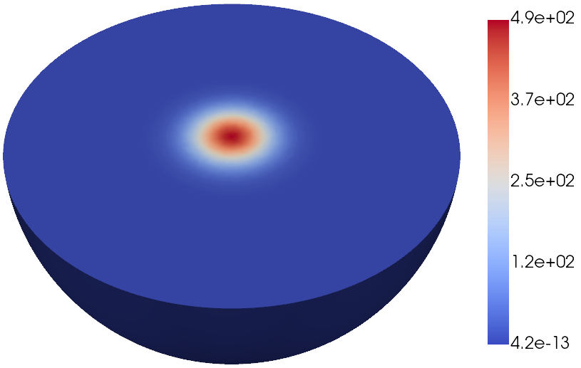
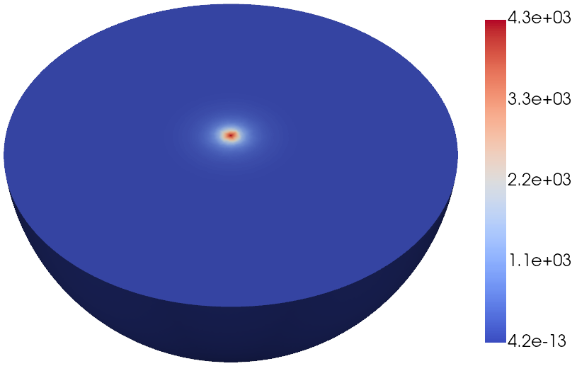
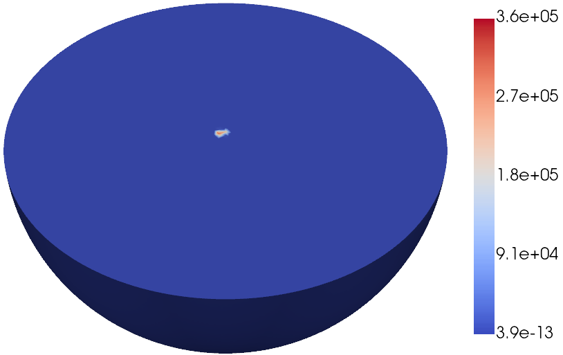
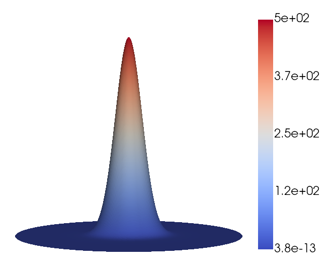
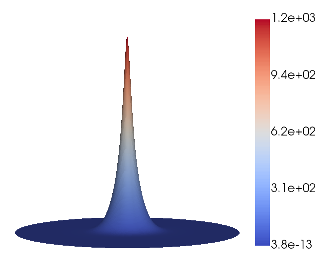
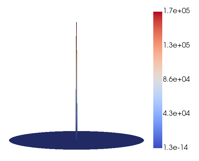
In this first example, we consider a 3D version ($n=3$) of model ($\mathcal{L}_{\tau}$) defined in the spatial domain $\Omega=\{(x,y,z)\in\mathbb{R}^{3}\colon x^{2}+y^{2}+z^{2}<1\}$ with the following initial condition

$$u_{0}(x,y,z)\coloneqq 500e^{-35(x^{2}+y^{2}+z^{2})},$$

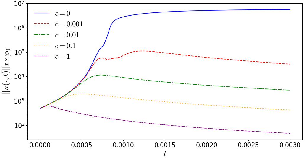
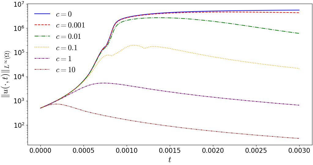
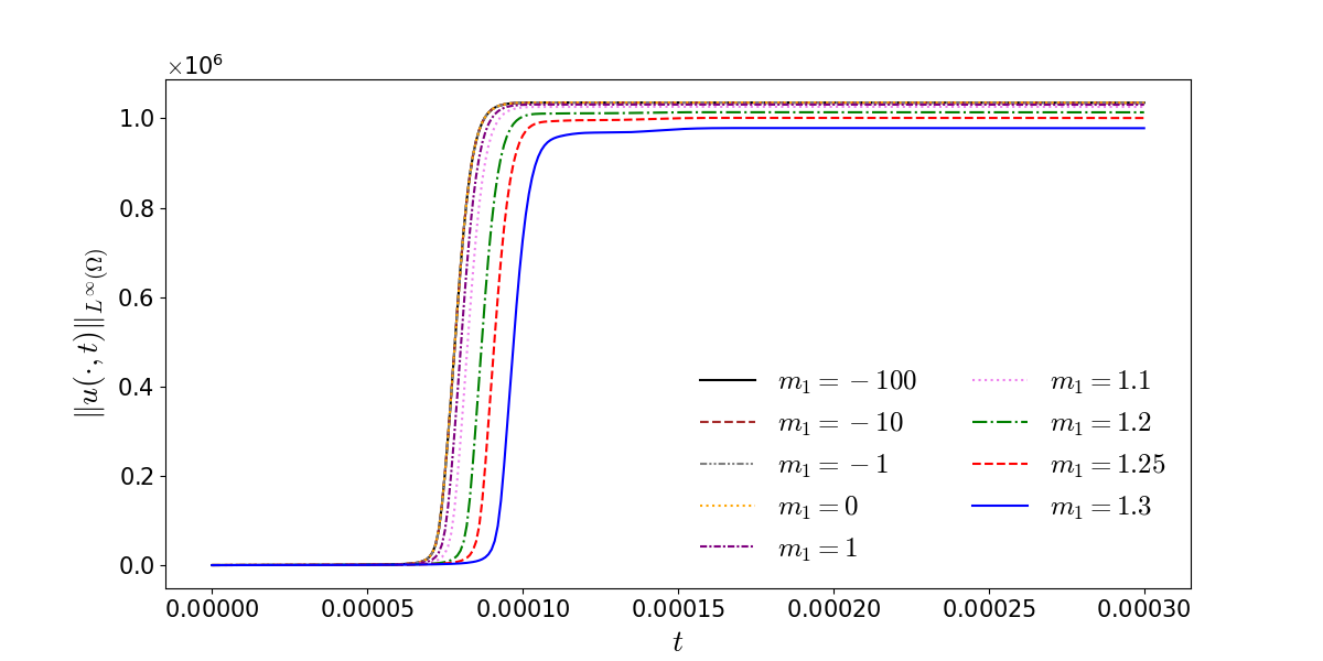
plotted in Figure 1a. Moreover, we take $\chi=5$ and $\xi=0$ (no repulsion) and we use a mesh of size $h\approx 4.4\cdot 10^{-2}$ and a time step $\Delta t=10^{-5}$. In Figure 1 the approximation obtained with $c=0$ is plotted at different time steps. We can observe that a blow-up phenomenon seems to appear (indeed, it is observable in Figures 1b and 1c how the maximum of the solution increases in the center of the sphere, eventually achieving the value $10^{5}$), according with the analytical results given in [54] – notice that $k=1.1<7/6\approx 1.167$ so the condition in [54, (1.4), Theorem 1.1] is satisfied. This blow-up phenomenon (interpretable in the sense of Criterion 1 in the next figures) can be prevented using appropriate damping gradient terms, as established in Theorem 2.2 (generalization of [21, Theorem 1.2]). As a matter of fact, we show in Figure 2 the evolution of the maximum of the approximations for different choices of $c$ and $\gamma$. Notice that the maximum shown in Figure 2 ($c=0$) achieves even higher values, up to the order $10^{6}$, than those exhibited in Figure 1 where a continuous, smoother, projection of the actual discontinuous approximated solution had been plotted. As expected, blow-up is prevented for whatever choice of $c>0$ (even for small values like $c=10^{-3}$) if $\gamma$ satisfies the bound $\mathcal{G}_{\tau}$, i.e., $1.5<\gamma\leq 2$ (see Figure 2a). However, in case that $\gamma$ does not comply with $\mathcal{G}_{\tau}$, we may require a big enough value of $c$ to prevent the gathering phenomena. This value of $c$, apparently breaking down the tendency toward chemotactic collapse, increases as long as $\gamma$ moves away from the value $\gamma^{*}=1.5$ for which the equality holds in $\mathcal{G}_{\tau}$ (see Figures 2b and 2c).

Refer to caption
a $t=0$.
Refer to caption
b $t=5\cdot 10^{-4}$.
Refer to caption
c $t=3\cdot 10^{-3}$.
Figure 1. Approximation of the solution $u$ at different time steps ($c=0$, $\chi=5$, $\xi=0$).
Refer to caption
a $\gamma=1.75$
Refer to caption
b $\gamma=1.4$.
Refer to caption
c $\gamma=1.1$.
Figure 2. Maximum of the approximation of $u$ over time for different values of $c$ and $\gamma$ ($\chi=5$, $\xi=0$).

7.2.2. Numerical simulations for the fully nonlinear attraction-repulsion model

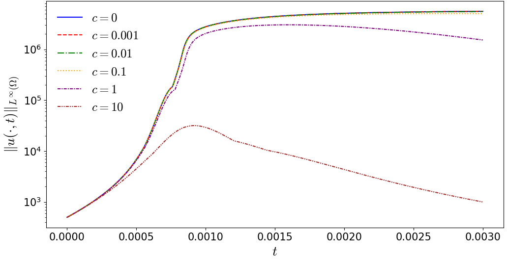
Motivated by [9], let us analyze model ($\mathcal{L}_{\tau}$) under the assumption that

(61) $$m_{2}=m_{3},m_{1}\in\mathbb{R},\alpha>\beta\quad\text{and}\quad\begin{cases}m_{2}+\alpha>\max\bigl{\{}m_{1}+\frac{2}{n}k,k\bigr{\}}&\text{ if }m_{1}\geq 0,\\ m_{2}+\alpha>\max\bigl{\{}\frac{2}{n}k,k\bigr{\}}&\text{ if }m_{1}<0.\end{cases}$$

In particular, we focus on the 2D case ($n=2$) in the domain $\Omega=\{(x,y)\colon x^{2}+y^{2}<1\}$. We set $\alpha=1.5$, $\xi=\chi=1$, and we define the following initial condition

$$u_{0}(x,y)\coloneqq 500e^{-35(x^{2}+y^{2})},$$

plotted in Figure 3a. Also, we take a spatial and a temporal partition of sizes $h\approx 1.37\cdot 10^{-2}$ and $\Delta t=10^{-6}$.

First, in Figure 3 we plot the evolution of $u$ over time without the damping gradient term, i.e., $c=0$. We observe that due to the choice of the parameters and the initial condition, it seems to occur a blow-up phenomenon (notable in Figures 3b and 3c), in accordance with the results in [9, Theorem 3] under restriction (61).

Refer to caption
a $t=0$.
Refer to caption
b $t=5\cdot 10^{-5}$.
Refer to caption
c $t=3\cdot 10^{-4}$.
Figure 3. Approximation of the solution $u$ at different time steps ($m_{1}=1$, $c=0$, $\alpha=1.5$).

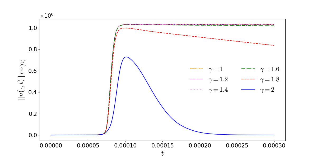
In fact, if we use a nonlinear diffusion term moving the value of $m_{1}$ we can observe in Figure 4 that we still obtain a chemotactic collapse but with times of explosion. Consistently to the real phenomenon, one may notice that the blow-up time increases (accordingly to Criterion 1) with $m_{1}$, the diffusion coefficient working against coalescence effects, specially for large values.

Refer to caption
Figure 4. Maximum of the approximation of $u$ for different values of $m_{1}$ ($c=0$, $\alpha=1.5$).

Moreover, as in the previous example, if we introduce the damping gradient nonlinearities using a strictly positive small value for $c$, such as $c=10^{-3}$, the blow-up phenomenon is avoided if we stick to the bounds on $\gamma$ given in $\mathcal{G}_{\tau}$, i.e., $1.67\approx 5/3<\gamma\leq 2$. However, this singularity seems to remain for a small enough value of $c$ if $\gamma$ does not satisfy $\mathcal{G}_{\tau}$; see Figure 5.

Refer to caption
Figure 5. Maximum of the approximation of $u$ for different values of $\gamma$ ($m_{1}=1$, $c=10^{-3}$, $\alpha=1.5$).

Acknowledgements

The research of TL is supported by NNSF of P. R. China (Grant No. 61503171), CPSF (Grant No. 2015M582091), and NSF of Shandong Province (Grant No. ZR2016JL021). The author DAS has been supported by UCA FPU contract UCA/REC14VPCT/2020 funded by Universidad de Cádiz and by a Graduate Scholarship funded by the University of Tennessee at Chattanooga. DAS also acknowledges the travel grants to visit the Università di Cagliari funded by the Universidad de Cádiz and the Erasmus KA+131 program. The authors AC and GV are members of the Gruppo Nazionale per l’Analisi Matematica, la Probabilità e le loro Applicazioni (GNAMPA) of the Istituto Nazionale di Alta Matematica (INdAM) and are partly supported by GNAMPA-INdAM Project Equazioni differenziali alle derivate parziali nella modellizzazione di fenomeni reali (CUP–E53C22001930001) and by Analysis of PDEs in connection with real phenomena (2021, Grant Number: F73C22001130007), funded by Fondazione di Sardegna. GV is also supported by MIUR (Italian Ministry of Education, University and Research) Prin 2022 Nonlinear differential problems with applications to real phenomena (Grant Number: 2022ZXZTN2). AC is also supported by GNAMPA-INdAM Project Problemi non lineari di tipo stazionario ed evolutivo (CUP–E53C23001670001).

References

  • [1] D. Acosta-Soba, F. Guillén-González, and J. R. Rodríguez-Galván. An Unconditionally Energy Stable and Positive Upwind DG Scheme for the Keller–Segel Model. J. Sci. Comput., 97(18), 2023.
  • [2] S. Badia, J. Bonilla, and J. V. Gutiérrez-Santacreu. Bound-preserving finite element approximations of the Keller–Segel equations. Math. Models Methods Appl. Sci., 33(03):609–642, 2023.
  • [3] H. Brezis. Functional Analysis, Sobolev Spaces and Partial Differential Equations, volume Universitext. Springer-Verlag, New York, 2011.
  • [4] A. Chertock and A. Kurganov. A second-order positivity preserving central-upwind scheme for chemotaxis and haptotaxis models. Numer. Math., 111(2):169–205, 2008.
  • [5] M. Chipot and F. B. Weissler. Some blowup results for a nonlinear parabolic equation with a gradient term. SIAM J. Math. Anal., 20(4):886–907, 1989.
  • [6] Y. Chiyo, F. G. Düzgün, S. Frassu, and G. Viglialoro. Boundedness through nonlocal dampening effects in a fully parabolic chemotaxis model with sub and superquadratic growth. Appl. Math. Optim., 89(9):1–21, 2024.
  • [7] Y. Chiyo, M. Marras, Y. Tanaka, and T. Yokota. Blow-up phenomena in a parabolic-elliptic-elliptic attraction-repulsion chemotaxis system with superlinear logistic degradation. Nonlinear Anal., 212, 2021.
  • [8] Y. Chiyo and T. Yokota. Boundedness and finite-time blow-up in a quasilinear parabolic-elliptic-elliptic attraction-repulsion chemotaxis system. Z. Angew. Math. Phys., 73(61):1–27, 2022.
  • [9] A. Columbu, S. Frassu, and G. Viglialoro. Properties of given and detected unbounded solutions to a class of chemotaxis models. Stud. Appl. Math., 151(4):1349–1379, 2023.
  • [10] D. A. Di Pietro and A. Ern. Mathematical aspects of discontinuous Galerkin methods, volume 69. Springer Science & Business Media, 2011.
  • [11] M. Fila. Remarks on blow up for a nonlinear parabolic equation with a gradient term. Proc. Amer. Math. Soc., 111(3):795–801, 1991.
  • [12] S. Frassu, R. Rodríguez Galván, and G. Viglialoro. Uniform in time ${L}^{\infty}$-estimates for an attraction-repulsion chemotaxis system with double saturation. Discrete Contin. Dyn. Syst. - B, 28(3):1886–1904, 2023.
  • [13] S. Frassu and G. Viglialoro. Boundedness for a fully parabolic Keller–Segel model with sublinear segregation and superlinear aggregation. Acta Appl. Math., 171(1):1–20, 2021.
  • [14] A. Friedman. Partial differential equations. Holt, Rinehart and Winston, Inc., New York-Montreal, Que.-London, 1969. Reprint, Dover Pubcications, Inc., Mineola-New York, 2008.
  • [15] M. Fuest. Approaching optimality in blow-up results for Keller–Segel systems with logistic-type dampening. Nonlinear Differ. Equ. Appl. NoDEA, 28(16):1–17, 2021.
  • [16] D. Gilbarg and N. Trudinger. Elliptic Partial Differential Equations of Second Order, 2nd ed. Springer-Verlag, Berlin, 1983.
  • [17] J. V. Gutiérrez-Santacreu and J. R. Rodríguez-Galván. Analysis of a fully discrete approximation for the classical Keller–Segel model: Lower and a priori bounds. Comput. Math. Appl., 85:69–81, 2021.
  • [18] M. A. Herrero and J. J. L. Velázquez. A blow-up mechanism for a chemotaxis model. Ann. Sc. Norm. Super. Pisa Cl. Sci. (4), 24(4):633–683, 1997.
  • [19] L. Hong, M. Tian, and S. Zheng. An attraction-repulsion chemotaxis system with nonlinear productions. J. Math. Anal. Appl., 484(1):123703, 2020.
  • [20] D. Horstmann and M. Winkler. Boundedness vs. blow-up in a chemotaxis system. J. Differ. Equ., 215(1):52–107, 2005.
  • [21] S. Ishida, J. Lankeit, and G. Viglialoro. A Keller–Segel type taxis model with ecological interpretation and boundedness due to gradient nonlinearities. Discrete Contin. Dyn. Syst. - B, 2024, doi:10.3934/dcdsb.2024029.
  • [22] W. Jäger and S. Luckhaus. On explosions of solutions to a system of partial differential equations modelling chemotaxis. Trans. Amer. Math. Soc., 329(2):819–824, 1992.
  • [23] G. J. O. Jameson. Some inequalities for $(a+b)^{p}$ and $(a+b)^{p}+(a-b)^{p}$. Math. Gaz., 98(541):96–103, 2014.
  • [24] B. Kawohl and L. A. Peletier. Observations on blow up and dead cores for nonlinear parabolic equations. Math. Z., 202(2):207–217, 1989.
  • [25] E. F. Keller and L. A. Segel. Initiation of slime mold aggregation viewed as an instability. J. Theoret. Biol., 26(3):399–415, 1970.
  • [26] E. F. Keller and L. A. Segel. Model for chemotaxis. J. Theoret. Biol., 30(2):225–234, 1971.
  • [27] E. F. Keller and L. A. Segel. Traveling bands of chemotactic bacteria: a theoretical analysis. J. Theoret. Biol., 30(2):235–248, 1971.
  • [28] O. A. Ladyženskaja, V. A. Solonnikov, and N. N. Ural’ceva. Linear and Quasi-Linear Equations of Parabolic Type. In Translations of Mathematical Monographs, volume 23. American Mathematical Society, 1988.
  • [29] J. Lankeit. Finite-time blow-up in the three-dimensional fully parabolic attraction-dominated attraction-repulsion chemotaxis system. J. Math. Anal. Appl., 504(2):125409, 2021.
  • [30] G. M. Lieberman. Hölder continuity of the gradient of solutions of uniformly parabolic equations with conormal boundary conditions. Ann. Mat. Pura Appl. (4), 148:77–99, 1987.
  • [31] D. Liu and Y. Tao. Boundedness in a chemotaxis system with nonlinear signal production. Appl. Math. J. Chinese Univ. Ser. B, 31(4):379–388, 2016.
  • [32] M. Liu and Y. Li. Finite-time blowup in attraction-repulsion systems with nonlinear signal production. Nonlinear Anal. Real World Appl., 61:103305, 2021.
  • [33] A. Lunardi. Analytic semigroups and optimal regularity in parabolic problems. Modern Birkhäuser Classics. Birkhäuser/Springer Basel AG, Basel, 1995.
  • [34] M. Marras, T. Nishino, and G. Viglialoro. A refined criterion and lower bounds for the blow-up time in a parabolic-elliptic chemotaxis system with nonlinear diffusion. Nonlinear Anal., 195:111725, 2020.
  • [35] M. S. Mock. An initial value problem from semiconductor device theory. SIAM J. Math. Anal., 5(4):597–612, 1974.
  • [36] M. S. Mock. Asymptotic behavior of solutions of transport equations for semiconductor devices. J. Math. Anal. Appl., 49(1):215–225, 1975.
  • [37] T. Nagai. Blowup of nonradial solutions to parabolic-elliptic systems modeling chemotaxis in two-dimensional domains. J. Inequal. Appl., 6(1):37–55, 2001.
  • [38] L. Nirenberg. On elliptic partial differential equations. Ann. Scuola Norm. Sup. Pisa Cl. Sci. (3), 2(13):115–162, 1959.
  • [39] P. Quittner and P. Souplet. Superlinear parabolic problems. Blow-up, global existence and steady states. Birkhäuser Advanced Texts: Basler Lehrbücher. Birkhäuser/Springer, Cham, 2019.
  • [40] G. Ren and B. Liu. Boundedness and stabilization in the 3D minimal attraction-repulsion chemotaxis model with logistic source. Z. Angew. Math. Phys., 73(58), 2022.
  • [41] M. W. Scroggs, J. S. Dokken, C. N. Richardson, and G. N. Wells. Construction of Arbitrary Order Finite Element Degree-of-Freedom Maps on Polygonal and Polyhedral Cell Meshes. ACM Trans. Math. Softw., 48(2), 2022.
  • [42] J. Shen and J. Xu. Unconditionally Bound Preserving and Energy Dissipative Schemes for a Class of Keller–Segel Equations. SIAM J. Numer. Anal., 58(3):1674–1695, 2020.
  • [43] P. Souplet. Finite time blow-up for a non-linear parabolic equation with a gradient term and applications. Math. Methods Appl. Sci., 19(16):1317–1333, 1996.
  • [44] P. Souplet. Recent results and open problems on parabolic equations with gradient nonlinearities. Electron. J. Differ. Equ., 2001(20):1–19, 2001.
  • [45] P. Souplet. The Influence of Gradient Perturbations on Blow-up Asymptotics in Semilinear Parabolic Problems: A Survey, pages 473–495. Birkhäuser Basel, Basel, 2005.
  • [46] Y. Tanaka. Boundedness and finite-time blow-up in a quasilinear parabolic–elliptic chemotaxis system with logistic source and nonlinear production. J. Math. Anal. Appl., 506(2):125654, 2022.
  • [47] Y. Tao and Z. A. Wang. Competing effects of attraction vs. repulsion in chemotaxis. Math. Models Methods Appl. Sci., 23(1):1–36, 2013.
  • [48] Y. Tao and M. Winkler. Boundedness in a quasilinear parabolic-parabolic Keller–Segel system with subcritical sensitivity. J. Differ. Equ., 252(1):692–715, 2012.
  • [49] G. Viglialoro. Blow-up time of A Keller–Segel-type system with Neumann and Robin boundary conditions. Differ. Integral Equ., 29(3-4):359–376, 2016.
  • [50] G. Viglialoro. Influence of nonlinear production on the global solvability of an attraction-repulsion chemotaxis system. Math. Nachr., 294(12):2441–2454, 2021.
  • [51] C. J. Wang, L. X. Zhao, and X. C. Zhu. A blow-up result for attraction-repulsion system with nonlinear signal production and generalized logistic source. J. Math. Anal. Appl., 518(1):126679, 2023.
  • [52] M. Winkler. Aggregation vs. global diffusive behavior in the higher-dimensional Keller–Segel model. J. Differential Equations, 248(12):2889–2905, 2010.
  • [53] M. Winkler. A critical blow-up exponent in a chemotaxis system with nonlinear signal production. Nonlinearity, 31(5):2031–2056, 2018.
  • [54] M. Winkler. Finite-time blow-up in low-dimensional Keller–Segel systems with logistic-type superlinear degradation. Z. Angew. Math. Phys., 69(40):1–25, 2018.
  • [55] M. Winkler and K. C. Djie. Boundedness and finite-time collapse in a chemotaxis system with volume-filling effect. Nonlinear Anal., 72(2):1044–1064, 2010.
  • [56] H. Yi, C. Mu, G. Xu, and P. Dai. A blow-up result for the chemotaxis system with nonlinear signal production and logistic source. Discrete Contin. Dyn. Syst. Ser. B, 26(5), 2021.
  • [57] X. Zhou, Z. Li, and J. Zhao. Asymptotic behavior in an attraction-repulsion chemotaxis system with nonlinear productions. J. Math. Anal. Appl., 507(1):125763, 2022.