Opening a meV mass window for Axion-like particles with a microwave-laser-mixed stimulated resonant photon collider

Abstract

We propose a microwave-laser-mixed three-beam stimulated resonant photon collider, which enables access to axion-like particles in the meV mass range. Collisions between a focused pulse laser beam and a focused microwave pulse beam directly produce axion-like particles (ALPs) and another focused pulse laser beam stimulates their decay. The expected sensitivity in the meV mass range has been evaluated. The result shows that the sensitivity can reach the ALP-photon coupling down to $\mathcal{O}(10^{-13})$ GeV^-1 with $10^{6}$ shots if 10-100 TW class high-intensity lasers are properly combined with a conventional 100 MW class S-band klystron. This proposal paves the way for identifying the nature of ALPs as candidates for dark matter, independent of any cosmological and astrophysical models.

I Introduction

Dark matter (DM) is one of the most intriguing unresolved problems in modern physics. Identifying DM in controlled experiments is thus an important subject. On the other hand, independently from such an astronomical and cosmological issue, elementary particle physics requires resolution to the strong CP problem. The topological nature of the QCD vacuum, $\theta$-vacuum, to solve the $U(1)_{A}$ anomaly naturally requires CP violating nature in the QCD Lagrangian. Nonetheless, the measured $\theta$-value in the neutron electric dipole moment suggests the CP conserving nature. To this non-trivial problem, Peccei and Quinn proposed a global $U(1)_{PQ}$ symmetry PQ . Through the symmetry breaking, a counter $\theta$-value can be dynamically produced and it cancels out the finite $\theta$-value. As a result of this symmetry breaking, axion with finite mass may appear AXION . If the energy scale of the symmetry breaking is much higher than that of the electroweak interaction, the coupling of axion to ordinary matter can be weak and thus such an invisible axion can be a quite rational candidate for low-mass dark matter Preskill:1982cy ; Abbott:1982af ; Dine:1982ah . Axion cosmology may have connections to the other unresolved problems in the standard model of elementary particle physics: finite neutrino mass and baryon number asymmetry and also in the cosmological problems: inflation and dark matter. Recently, extended SU(5) grand unified theory (GUT) SU5U1pq and SO(10) GUT SO10U1pq by adding $U(1)_{PQ}$ to solve the strong CP problem are discussed as an approach to access these unresolved issues within one stroke. Cosmological observations, particularly those derived from cosmic microwave background data sensitive to the early-stage evolution of the Universe, present an opportune moment to refine our understanding by constraining the relevant parameter spaces associated with specific phenomena. This can be achieved through the establishment of connections between these phenomena, guided by the overarching framework of spontaneous symmetry breaking. Such an approach unifies the disparate elements by identifying relevant symmetries across different evolutionary stages.

There is an unexplored mass range around meV in the photon-axion coupling predicted by the benchmark QCD axion models. Furthermore, the unified inflaton and dark matter model (miracle) Miracle1 ; Miracle2 predicts an axion-like particle (ALP) in the photon-ALP coupling $\mathcal{O}(10^{-10}-10^{-13})$ $\mbox{GeV}^{-1}$ in the allowed ALP mass range $\mathcal{O}(10^{-3}-10^{2})$ eV based on the viable parameter space consistent with the CMB observation. Thus, opening a search window in the meV mass range would increase the potential to discover axion and ALPs.

Historically, hallo-scope ADMX and helio-scope CAST have spearheaded the quest for axions and axion-like particles (ALPs), boasting the highest sensitivities to date. Nonetheless, while these observations may potentially detect manifestations of ALP decays in the future, discerning the spin and parity states of dark matter would pose a formidable challenge. Therefore, as complementary observations, we have proposed stimulated resonant photon colliders (SRPC) using coherent electromagnetic fields with two beams DEptp ; JHEP2020 and with three beams 3beam00 , respectively. The method is to directly produce ALPs and simultaneously stimulate their decays by combining several laser fields. Quasi-parallel SRPC with two laser beams has been dedicated for the sub-eV axion mass window and the searches have been actually performed PTEP2014 ; PTEP2015 ; PTEP2020 ; SAPPHIRES00 ; SAPPHIRES01 . In contrast, SRPC with large incident angles of three laser beams has a potential to be sensitive to higher mass 3beam00 ; 3beam01 ; 3beam02 compared to the two beam case.

In this paper we propose an extremely asymmetric three-beam collider by combining a microwave beam from a klystron and two short pulse laser beams in order to open a search window for meV-scale ALPs. We then provide the expected sensitivity based on a practical set of beam parameters.

II Kinematical relations in extremely asymmetric stimulated three beam collider

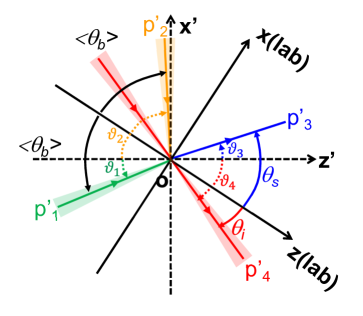
Figure 1: Angle relations in a three beam collider between laboratory coordinates and zero transverse momentum coordinates with the primed symbol. Colored cones represent focused beams at the common focal point (O): $p^{{}^{\prime}}_{1}$ and $p^{{}^{\prime}}_{2}$ denote two incident photon momenta from the two creation beams without drawing the diverging parts of the beams while $p^{{}^{\prime}}_{4}$ indicates a photon momentum from the inducing beam with the focusing and diverging beam. As a result of the interaction, a signal photon, $p^{{}^{\prime}}_{3}$, is emitted. Although angles of these four photons may deviate from the individual beam axes due to the uncertainty principles, the peculiar case where all the photons coincide with the beam axes is on purpose displayed to introduce the angle definitions in the two coordinate systems. Since a target mass gives a bisecting angle $\langle\vartheta_{b}\rangle$ between the two creation beam axes, the bisecting axis can be a natural $z$-coordinate as the laboratory coordinates. Further details can be found in the main text.

We consider photon-photon collisions to produce an ALP resonance state between a focused short-pulse laser beam (green) and a focused microwave pulse beam (orange) as illustrated in Fig.1. Simultaneously we focus another short-pulse laser beam (red) into the collision point in order to induce decay of the resonantly produced ALP. In the case of collisions between tightly focused photon beams, at around the focal region, individual photon momenta must follow the uncertainty principle in the momentum-position relation. In addition, in the case of short pulsed beams, the uncertainty on the energy-time relation must also be taken into account. Therefore, we consider the stimulated photon-photon scattering process by including stochastic selections of photons from the focused fields with different momenta and energies from the central values of those in the three beams. Suppose four-momenta $p_{1}$ and $p_{2}$ from the incident laser and microwave beams, respectively, for the resonance creation part and $p_{4}$ from the inducing laser beam. The signal photon is then defined as $p_{3}$ as a result of ALP decay into $p_{3}+p_{4}$. For a given pair of $p_{1}$ and $p_{2}$, we are allowed to arbitrarily set an axis to which incident angles are relatively defined. In such arbitrary coordinates, with the energies of four photons $\omega_{j}$ and scattering angles $\vartheta_{j}$ for initial $j=1,2$ and final $j=3,4$ states, four-momenta are defined as follows:

$$p_{1} =( \omega_{1}, \omega_{1}\sin\vartheta_{1}, 0, \omega_{1}\cos\vartheta_{1})$$ , (1)

$$p_{2} =( \omega_{2}, -\omega_{2}\sin\vartheta_{2}, 0, \omega_{2}\cos\vartheta_{2})$$ ,

$$p_{3} =( \omega_{3}, \omega_{3}\sin\vartheta_{3}, 0, \omega_{3}\cos\vartheta_{3})$$ ,

$$p_{4} =( \omega_{4}, -\omega_{4}\sin\vartheta_{4}, 0, \omega_{4}\cos\vartheta_{4}).$$

For later convenience, a bisecting angle $\vartheta_{b}$ is further introduced as

$$\vartheta_{b}\equiv\frac{\vartheta_{1}+\vartheta_{2}}{2}.$$ (2)

The energy-momentum conservation requires following relations

$$\omega_{1}+\omega_{2} =\omega_{3}+\omega_{4}$$ (3)

$$\omega_{1}\cos\vartheta_{1}+\omega_{2}\cos\vartheta_{2} =\omega_{3}\cos\vartheta_{3}+\omega_{4}\cos\vartheta_{4}\equiv\omega_{z}$$

$$\omega_{1}\sin\vartheta_{1}-\omega_{2}\sin\vartheta_{2} =\omega_{3}\sin\vartheta_{3}-\omega_{4}\sin\vartheta_{4}\equiv\omega_{x}.$$

The corresponding center-of-mass system energy, $E_{cms}$, is then expressed as

$$E_{cms}=\sqrt{(p_{1}+p_{2})^{2}}=\sqrt{2\omega_{1}\omega_{2}\{1-\cos(\vartheta_{1}+\vartheta_{2})\}}=2\sqrt{\omega_{1}\omega_{2}}\sin\vartheta_{b}{}.$$ (4)

For a given ALP mass $m_{a}$, the resonance condition is defined as

$$m_{a}=E_{cms}=2\sqrt{\omega_{1}\omega_{2}}\sin\vartheta_{b}{}.$$ (5)

From Eqs.(3) and (5), we can derive the following relations by utilizing the fact that massless photons must satisfy the conditions ${p_{3}}^{2}={p_{4}}^{2}=0$, that is,

$${p_{3}}^{2}=m^{2}_{a}-2\omega_{4}(\omega_{1}+\omega_{2}+\omega_{x}\sin\vartheta_{4}-\omega_{z}\cos\vartheta_{4})=0$$ (6)

$${p_{4}}^{2}=m^{2}_{a}-2\omega_{3}(\omega_{1}+\omega_{2}-\omega_{x}\sin\vartheta_{3}-\omega_{z}\cos\vartheta_{3})=0.$$

Among possible choices of a colliding axis, theoretically beneficial one is the axis to which the transverse momentum sum, $p_{T}$, between $p_{1}$ and $p_{2}$ vanishes, corresponding to the case of $\omega_{x}=0$ in Eq.(3). In the zero-$p_{T}$ coordinates, hereafter denoted with the prime symbol, the solid angle integral in the final state photons is greatly simplified because $p_{3}$ and $p_{4}$ must also symmetrically distribute around this common axis. On the other hand, an experimentally convenient collision axis is the bisecting axis to which the laser and microwave beam axes can be symmetrically aligned. We thus introduce the laboratory coordinates $(t,x,y,z)$ so that the bisecting axis corresponds to the $z$-axis where all the central beam axes are co-planer in the $x-z$ plane and the origin of time $t$ is set at the moment when the pulse peak positions of the three beams simultaneously arrive at the common focal spot.

For the experimental setup, we introduce the central values for the photon energies as $\omega_{c_{1}}=\langle\omega_{1}\rangle$, $\omega_{c_{2}}=\langle\omega_{2}\rangle$, $\omega_{s}=\langle\omega_{3}\rangle$, and $\omega_{i}=\langle\omega_{4}\rangle$ where $\langle\quad\rangle$ denotes taking central values of individual distributions. These are a priori known parameters for a given target ALP mass $\langle m_{a}\rangle=2\sqrt{\omega_{c_{1}}\omega_{c_{2}}}\sin\langle\vartheta_{b}\rangle$. In order to obtain the incident angle for the central axis of the inducing beam $\langle\vartheta_{4}\rangle$ and the corresponding emission angle of the induced decay signal photon $\langle\vartheta_{3}\rangle$, we apply the zero-$p_{T}$ coordinates to the central beam incident angles with the central beam energies, that is, in the case of $\omega_{x}=0$. From $\omega_{1}\sin\vartheta_{1}=\omega_{2}\sin\vartheta_{2}$ with $\vartheta_{2}=2\vartheta_{b}-\vartheta_{1}$ due to $\omega_{x}=0$, the following relation on $\vartheta_{1}(>0)$ is obtained

$$\vartheta_{1}=\sin^{-1}\left(\frac{\sin 2\vartheta_{b}}{\sqrt{(\frac{\omega_{1}}{\omega_{2}}+\cos 2\vartheta_{b})^{2}+\sin^{2}2\vartheta_{b}}}\right).$$ (7)

The central value of $\omega_{z}$, $\overline{\omega_{z}}$, is calculable from Eq.(6) with the individual central parameters. The central angles are then expressed as

$$\langle\vartheta_{3}\rangle=\cos^{-1}\left(\frac{1}{\overline{\omega_{z}}}(\omega_{c_{1}}+\omega_{c_{2}}-\frac{{\langle m_{a}\rangle}^{2}}{2\omega_{s}})\right)$$ (8)

$$\langle\vartheta_{4}\rangle=\cos^{-1}\left(\frac{1}{\overline{\omega_{z}}}(\omega_{c_{1}}+\omega_{c_{2}}-\frac{{\langle m_{a}\rangle}^{2}}{2\omega_{i}})\right).$$

As denoted in Fig.1, the offset angle from the bisecting axis to the zero-$p_{T}$ axis is $\vartheta_{b}-\vartheta_{1}$. With the offset, we eventually define the nominal emission angle of signal photons and the incident angle of the inducing beam in the laboratory coordinates as

$$\vartheta_{s}\equiv\langle\vartheta_{3}\rangle+(\langle\vartheta_{b}\rangle-\langle\vartheta_{1}\rangle)$$ (9)

$$\vartheta_{i}\equiv\langle\vartheta_{4}\rangle-(\langle\vartheta_{b}\rangle-\langle\vartheta_{1}\rangle).$$

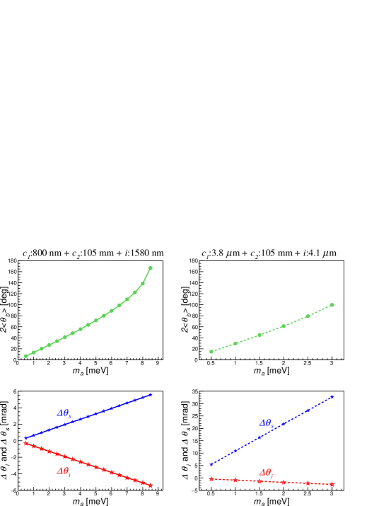
Figure 2: Kinematically allowed incident angles of three beams for higher (solid curves) and lower mass (dotted curves) options. Left top-bottom panels are for the higher mass option consisting of the first creation beam $c_{1}$: 800 nm (laser), second creation beam $c_{2}$: 105 mm (S-band microwave) and inducing beam $i$: 1580 nm (laser). Right top-bottom panels are for the lower mass option consisting of the first creation beam $c_{1}$: 3.8 $\mu$m (laser), the second creation beam$c_{2}$: 105 mm (S-band microwave) and the inducing beam $i$: 4.1 $\mu$m (laser). Top two panels: $c_{1}$-beam incident angles with respect to those of $c_{2}$-beam, that is, $2\langle\vartheta_{b}\rangle$ as a function of targe ALP mass $\langle m_{a}\rangle$. Bottom two panels: signal emission angles and incident angles of the inducing beam relative to incident angles of the $c_{1}$ beam as a function of target ALP mass $\langle m_{a}\rangle$.

An asymmetric combination between $\omega_{1}=O(1)$ eV and $\omega_{2}=O(10^{-5})$ eV gives $E_{cms}=O(10^{-3})$ eV by adjusting the subtended angle $2\langle\vartheta_{b}\rangle$. In this case, however, the actual collision geometry is quite different from Fig.1 (see Fig.3) which merely displays the defined relation between the incident angles of the beams and the emission angle of signals.

In this proposal we consider the following two combinations of three beams for higher and lower mass options. The higher mass search consists of the first creation beam $c_{1}$: 800 nm (laser), the second creation beam $c_{2}$: 105 mm (S-band microwave) and the inducing beam $i$: 1580 nm (laser), while the lower mass search is the combination of the first creation beam $c_{1}$: 3.8 $\mu$m (laser), the second creation beam $c_{2}$: 105 mm (S-band microwave) and the inducing beam $i$: 4.1 $\mu$m (laser). Figure 2 shows kinematically allowed incident angles of three beams for the higher (solid curves) and the lower mass (dotted curves) options. The top two panels show that $c_{1}$-beam incident angles with respect to $c_{2}$-beam, that is, $2\langle\vartheta_{b}\rangle$ as a function of targe ALP mass $\langle m_{a}\rangle$. The bottom two panels display that signal emission angles and incident angles of the inducing beam relative to incident angles of the $c_{1}$ beam as a function of target ALP mass $\langle m_{a}\rangle$. As shown in the bottom panels, angle differences of inducing beam incident angles $\langle\theta_{i}\rangle$ and those of signal photon emission angles $\langle\theta_{s}\rangle$ commonly relative to $c_{1}$-beam incident angles span $\cal{O}$(1-10) mrad. This indicates peculiar collision geometries where the creation and inducing laser beams are almost parallel but must have slightly different intersection angles. Since divergence angles of typical lasers can be sub-mrad and the pointing stability can be guaranteed, it is feasible to precisely control the relative incident angles. The signal emission angles are also almost aligned with the $c_{1}$-beam incident angles. Because the signal photon energy $\omega_{s}=\omega_{c_{1}}+\omega_{c_{2}}-\omega_{i}\sim\omega_{c_{1}}-\omega_{i}$ due to $\omega_{c_{1}},\omega_{i}\gg\omega_{c_{2}}$ is very different from any of $\omega_{c_{1}},\omega_{c_{2}},\omega_{i}$, the signal photons can be separated from those of the incident laser beams by reflecting them to another direction via a set of dichroic mirrors (see Fig.3), which has been demonstrated in the actual experimental setups in PTEP2014 ; PTEP2015 ; PTEP2020 ; SAPPHIRES00 ; SAPPHIRES01 .

III Conceptual design for a variable angle three beam collider

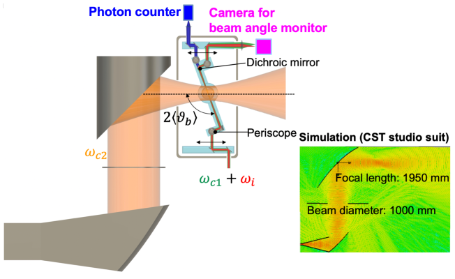
Figure 3: Left: schematic drawing for an experimental setup to combine laser beams and a microwave beam for the search for meV ALPs. The creation beam line by focusing microwaves ($c_{2}$) from a S-band klystron is taken to be fixed, while the creation laser beam ($c_{1}$) and the inducing laser beam $(i)$ with small intersecting angles to $c_{1}$ are arbitrary rotated all together on the same turning table. As indicated in the bottom plots in Fig.2, signal photons and inducing beams are almost aligned with the creation laser beam $c_{1}$. The almost co-moving laser beams are reflected on a dichroic mirror in order to separate signal photons (blue) from the intense used laser beams. The incident laser beams are monitored by a camera which measures the individual focal positions so that the slight intersecting angles between the two lasers can be measured in order to ensure the correct kinematical relation. The signal photons are collected and counted by a single-photon sensitive photodetector. Right: simulation result on the S-band microwave focusing. The result using CST Studio Suite CST shows that a focal distance around 2 m is indeed feasible if a proper horn and an aperture are equipped in addition to the focusing parabolic mirror.

Given the kinematical relations between three beams in the previous section, we envision a searching setup for scanning the meV mass range as depicted in Fig.3, where a microwave photon beam ($c_{2}$: 105 mm) from a S-band (2.856 GHz) klystron is assumed to be focused from a fixed position, while incident angles of a creation laser beam ($c_{1}$: 800 nm / 3800 nm) and an inducing laser beam (i: 1580 nm / 4100 nm) are variably controlled. The wavelength of 800 nm is available using well-known Ti:Sapphire lasers and the high-intensity lasers are available worldwide ELI , the wavelength around 4 $\mu$m can be produced with solid-state lasers based on iron-doped zinc selenide (Fe:ZnSe) currently attracting significant attention as efficient and powerful sources in the mid-infrared (MIR) spectral region Tokita . The wavelengths of the individual inducing lasers can be generated via optical parametric amplification by pumping the corresponding creation lasers with respect to proper seed lasers. Therefore, there is some degree of choice for signal wavelengths corresponding to $\omega_{c_{1}}-\omega_{i}$. By introducing the two combinations of the laser fields, the meV mass window can be enlarged. Focusing of a S-band microwave beam in a short distance is not a trivial issue. We thus performed the simulation using CST Studio Suite CST , which is shown in the right figure. We conclude that a focal distance around 2 m is feasible if a proper horn and an aperture are equipped in addition to the focusing parabolic mirror. Since the incident angles of the two laser beams and the signal photon emission angle are almost aligned, a rotating table accommodating the two beams and a dichroic mirror reflecting the two beams to a different direction from the signal’s one can be implemented. The signal photons are assumed to be counted by a single-photon-sensitive photodevice, while the two laser beams sent outside the chamber are further focused into a camera so that the focal points of the two beams can be monitored to guarantee the accurate incident angle relations. According to rotation angles of the table, a sliding mirror and the top-bottom mirrors in the periscope locally rotate so that incident points of the two lasers to the entrance window of the interaction chamber can remain unchanged.

IV Signal yield in stimulated resonant photon scattering

We address the following effective Lagrangian describing the interaction of an ALP as a pseudoscalar field $\phi_{a}$ with two photons

$$-{\cal L}=\frac{1}{4}\frac{g}{M}F_{\mu\nu}\tilde{F}^{\mu\nu}\phi_{a},$$ (10)

using dimensionless coupling $g$, an energy scale for symmetry breaking $M$, electromagnetic field strength tensor $F_{\mu\nu}$ and its dual $\tilde{F}^{\mu\nu}$. The comprehensive derivation of the scattering amplitude for stimulated resonant photon scattering applicable to the most general collision geometry is elaborated upon in  JHEP2020 ; Universe00 . Further elucidation regarding the implementation of these formulations in the context of a three-beam collision scenario, featuring two equivalent incident energies at symmetric incident angles with an inducing beam, is presented in 3beam00 . Hereafter, we outline the formulation by reviewing the pertinent sections in order to evaluate the expected sensitivity in the collision case characterized by two highly disparate incident energies and asymmetric incident angles with an inducing beam.

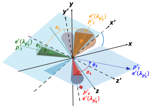
Figure 4: Relations between laboratory coordinates and theoretical coordinates with the primed symbol. The central axes of the three beams are physically placed on the x-z plane in laboratory coordinates in the co-planer condition. Theoretically a $z^{{}^{\prime}}$-axis is calculable so that stochastically selected two incident photons satisfying the resonance condition have zero pair transverse momentum ($p_{T}$) with respect to $z^{{}^{\prime}}$. The Lorentz invariant scattering amplitude is calculated on the primed coordinates where rotation symmetries of the initial and final state reaction planes (sky blue) around $z^{{}^{\prime}}$ are guaranteed. Notations of four-momentum vectors $p^{\prime}_{j}$ and four-polarization vectors $e^{\prime}(\lambda_{p^{\prime}_{j}})$ with polarization states $\lambda_{p^{\prime}_{j}}$ for the initial state ($j=1,2$) and final state ($j=3,4$) plane waves are displayed.

The relation between theoretical coordinates with the primed symbol and laboratory coordinates to which colliding beams are physically mapped is illustrated in Fig.4. By taking the momentum uncertainty, that is, the incident angle uncertainty into account, we have to accept a situation where reaction planes between pairs of incident photons from the two beams most likely deviate from the co-planar plane including the three beams, that is, $x-z$ plane. As illustrated in Fig.4, we thus introduce zero transverse momentum coordinates (zero-$p_{T}$) where the total transverse momentum of an incident pair (and outgoing pair) of photons becomes zero, as a basis for the calculation of the photon-photon scattering amplitude. We define the $z^{{}^{\prime}}$-axis as the direction of the summed vector of the incident pair of photons in the zero-$p_{T}$ coordinates by adding the transverse $x^{{}^{\prime}}$-axis aligned to the $p_{T}$ direction so that the pair vectors are contained in the $x^{{}^{\prime}}-z^{{}^{\prime}}$ plane. The zero-$p_{T}$ coordinates provides the axial symmetry around the $z^{{}^{\prime}}$-axis, thus, simplifies the calculation for the interaction rate with stimulation by the inducing beam. Once we calculate the rate, the positions of signal photons can be calculated by rotating zero-$p_{T}$ coordinates back to the laboratory coordinates.

The Lorentz invariant scattering amplitude is computed in the primed coordinates, where the rotational symmetries of the initial and final state reaction planes around $z^{{}^{\prime}}$ are preserved. Notations of four-momentum vectors $p^{\prime}_{j}$ and four-polarization vectors $e^{\prime}(\lambda_{p^{\prime}_{j}})$ with polarization states $\lambda_{p^{\prime}_{j}}$ for the initial-state ($j=1,2$) and final-state ($j=3,4$) plane waves, are displayed. The conversion between the two coordinate systems is achievable through a straightforward rotation $\cal{R}$, as elaborated below. Henceforth, unless ambiguity arises, the prime symbol associated with the momentum vectors will be omitted.

We commence by examining the spontaneous emission yield of the signal $p_{3}$, denoted as $\mathcal{Y}$, within the scattering process $p_{1}+p_{2}\rightarrow p_{3}+p_{4}$, utilizing solely two incident photon beams characterized by normalized number densities $\rho_{1}$ and $\rho_{2}$ with average numbers of photons $N_{1}$ and $N_{2}$ for pulse 1 and 2, respectively. The notion of ”cross section” proves beneficial when the beams of $p_{1}$ and $p_{2}$ remain fixed. Nonetheless, in scenarios where the momenta of $p_{1}$ and $p_{2}$ exhibit significant fluctuations within the beams, the utility of this concept diminishes BJ . Instead of ”cross section”, we hereby introduce the refined expression for ”volume-wise interaction rate” denoted as $\overline{\Sigma}$ PTEP2014 , measured in units of length ($L$) and time ($s$), indicated as $[\quad]$:

$${\mathcal{Y}}=N_{1}N_{2}\left(\int dtd\bm{r}\rho_{1}(\bm{r},t)\rho_{2}(\bm{r},t)\right)\times\mbox{\hskip 56.9055pt}$$ (11)

$$\left(\int dQW(Q)\frac{c}{2\omega_{1}2\omega_{2}}|{\mathcal{M}}_{s}(Q^{{}^{\prime}})|^{2}dL^{{}^{\prime}}_{ips}\right)\mbox{\hskip 5.69046pt}$$

$$\equiv N_{1}N_{2}{\mathcal{D}}\left[s/L^{3}\right]\overline{\Sigma}\left[L^{3}/s\right]\mbox{\hskip 93.89418pt}$$ (12)

with the velocity of light $c$ and the Lorentz-invariant phase space factor $dL_{ips}$

$$dL_{ips}=(2\pi)^{4}\delta(p_{3}+p_{4}-p_{1}-p_{2})\frac{d^{3}p_{3}}{2\omega_{3}(2\pi)^{3}}\frac{d^{3}p_{4}}{2\omega_{4}(2\pi)^{3}}.$$ (13)

Here, the probability density of the center-of-mass system energy, $W(Q)$, is incorporated to yield the average across the feasible range of $Q$. For the incident beams $\alpha=1$ and $2$, $W(Q)$ is defined as a function of the combinations of photon energies($\omega_{\alpha}$), polar($\Theta_{\alpha}$) and azimuthal($\Phi_{\alpha}$) angles in laboratory coordinates, which is denoted as

$$Q\equiv\{\omega_{\alpha},\Theta_{\alpha},\Phi_{\alpha}\}\quad\mbox{and}\quad dQ\equiv\Pi_{\alpha}d\omega_{\alpha}d\Theta_{\alpha}d\Phi_{\alpha}.$$ (14)

The integral, weighted by $W(Q)$, embodies the resonance enhancement by incorporating both the off-shell component and the pole within the s-channel amplitude corresponding to the Breit-Wigner resonance function included in $|{\mathcal{M}}_{s}(Q^{{}^{\prime}})|^{2}$ with spin states $s$ defined through combinations of four-polarization vectors $e^{\prime}(\lambda_{p^{\prime}_{j}})$ for $j=1,2,3,4$ JHEP2020 . As depicted in Fig.4, $Q^{{}^{\prime}}\equiv{\omega_{\alpha},\vartheta_{\alpha},\phi_{\alpha}}$ represent kinematical parameters within a rotated coordinate system $Q^{{}^{\prime}}$, constructed from a pair of incident wave vectors such that the transverse momentum of the pair, relative to a $z^{{}^{\prime}}$-axis, is nullified. The conversion from $Q$ to $Q^{{}^{\prime}}$ is thus delineated by rotation matrices acting upon polar and azimuthal angles: $\vartheta_{\alpha}\equiv{\cal R}_{\vartheta_{\alpha}}(Q)$ and $\phi_{\alpha}\equiv{\cal R}_{\phi_{\alpha}}(Q)$.

By introducing an inducing beam characterized by the central four-momentum $p_{4}$, possessing the normalized number density denoted as $\rho_{4}$ and the averaged photon number of photons, $N_{4}$, we broaden the scope of the spontaneous yield to encompass the induced yield, denoted as ${\cal Y}_{c+i}$, incorporating an expanded set of kinematical parameters as delineated below:

$${\mathcal{Y}}_{c+i}=N_{1}N_{2}N_{4}\left(\int dtd\bm{r}\rho_{1}(\bm{r},t)\rho_{2}(\bm{r},t)\rho_{4}(\bm{r},t)V_{4}\right)\times\mbox{\hskip 19.91684pt}$$ (15)

$$\left(\int dQ_{I}W(Q_{I})\frac{c}{2\omega_{1}2\omega_{2}}|{\mathcal{M}}_{s}(Q^{{}^{\prime}})|^{2}dL^{{}^{\prime}I}_{ips}\mbox{\hskip 2.84544pt}\right)$$

$$\equiv N_{1}N_{2}N_{4}{\mathcal{D}}_{exp}\left[s/L^{3}\right]\overline{\Sigma}_{I}\left[L^{3}/s\right]\mbox{\hskip 88.2037pt}$$

with

$$Q_{I}\equiv\{Q,\omega_{4},\Theta_{4},\Phi_{4}\}\quad\mbox{and}\quad dQ_{I}\equiv dQd\omega_{4}d\Theta_{4}d\Phi_{4},$$ (16)

where the factor $\rho_{4}(\bm{r},t)V_{4}$ represents a probabilistic measure indicative of the extent of spatiotemporal alignment between the $p_{1}$ and $p_{2}$ beams and the inducing beam $p_{4}$, within the specified volume $V_{4}$ of the $p_{4}$ beam. Meanwhile, $dL^{{}^{\prime}I}_{ips}$ expresses an inducible phase space wherein the solid angles of $p_{3}$ balance with those of $p_{4}$, ensuring conservation of energy-momentum within the distribution of the inducing beam. This entails the conversion of $p_{4}$ from the primed coordinate system to the corresponding laboratory coordinates, where the three beams are physically mapped in order to estimate the effective enhancement factor due to the inducing effect. With Gaussian distributions denoted as $G$, the function $W(Q_{I})$ is precisely characterized as:

$$W(Q_{I})\equiv\Pi_{\beta}G_{E}(\omega_{\beta})G_{p}(\Theta_{\beta},\Phi_{\beta})$$ (17)

for $\beta=1,2,4$. Here, $G_{E}$, reflecting an energy spread due to the Fourier transform-limited duration of a short pulse, and $G_{p}$, representing the momentum space or equivalently the polar angle distribution, are introduced. These distributions are based on the properties of a focused coherent electromagnetic field with axial symmetric characteristics concerning the azimuthal angle $\Phi_{\beta}$ around the optical axis of focused beam $\beta$.

Integrating Eq.(15) analytically is not practical. Thus the numerical integral is performed. The detailed algorithm for the integral of $\overline{\Sigma}_{I}$ is provided in  JHEP2020 ; 3beam00 , while the quasi-analytic expression for the generalized density overlapping factor ${\mathcal{D}}_{exp}$ in Eq.(15) adaptable to real experimental conditions is provided in Appendix of this paper.

V Sensitivity projection

We now evaluate the expected sensitivity with the given expression for the signal yield. Table 1 summarizes assumed beam relevant parameters for $c_{1}$, $c_{2}$, and $i$ as well as the statistical parameters. For the set of the beam parameters $P$ in Tab. 1, the number of signal photons, $N_{obs}$, in the three-beam stimulated resonant photon scattering process is expressed as

$$N_{obs}={\cal Y}_{c+i}(m_{a},g/M;P)N_{shot}\epsilon$$ (18)

as a function of ALP mass $m_{a}$ and coupling $g/M$ with the number of laser shots, $N_{shot}$, and the overall efficiency for detecting $p_{3}$, $\epsilon$. For a set of $m_{a}$ values with assumed $N_{obs}$, a set of coupling $g/M$ can be obtained by numerically solving Eq.(18).

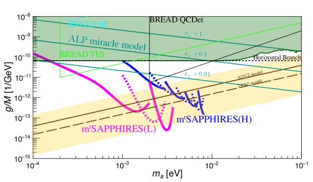
Figure 5: Expected sensitivities in the coupling-mass relation for the pseudoscalar field exchange at a 95% confidence level by a three-beam stimulated resonant photon collider combining two laser beams and a microwave beam from a S-band klystron. The used beam parameters are summarized in Table 1. The thick solid/dashed curves show the expected upper limits by the proposed laser-microwave-mixed three-beam stimulated resonant photon collider (m^tSAPPHIRES) with the parameter set in Tab.1. m^tSAPPHIRES(H) (blue) denotes the combination between $c_{1}$: 800 nm, $c_{2}$: S-Band, and $i$: 1580 nm, while m^tSAPPHIRES(L) (magenta) corresponds to the combination between $c_{1}$: 3800 nm, $c_{2}$: S-Band, and $i$: 4100 nm. Further details can be found in the main text.

With the parameter values in Table 1, Fig.5 shows the sensitivity projection in the coupling-mass relation for the pseudoscalar field exchange at a 95% confidence level.

These sensitivity curves are derived under the following conditions. In this simulated exploration, the null hypothesis assumes fluctuations in the count of photon-like signals, adhering to a Gaussian distribution with an expected value of zero for the provided total collision statistics. The term ”photon-like signals” denotes instances where peaks resembling photons are enumerated through a peak-finding algorithm applied to digitized waveform data obtained from a photodetector SAPPHIRES00 . Here, electrical fluctuations around the waveform’s baseline yield both positive and negative counts of photon-like signals.

To reject this null hypothesis, a confidence level $1-\alpha$ is defined as

$$1-\alpha=\frac{1}{\sqrt{2\pi}\sigma}\int^{\mu+\delta}_{\mu-\delta}e^{-(x-\mu)^{2}/(2\sigma^{2})}dx=\mbox{erf}\left(\frac{\delta}{\sqrt{2}\sigma}\right),$$ (19)

where $\mu$ represents the expected value of an estimator $x$ following the hypothesis, and $\sigma$ denotes one standard deviation. In this investigation, the estimator $x$ corresponds to the count of signal photons $N_{S}$ and we presume the uncertainty, $\delta N_{S}$, uncorrected for detector acceptance, to represent one standard deviation $\sigma$ around the mean value $\mu=0$. In order to set a confidence level of 95%, $2\alpha=0.05$ with $\delta=2.24\sigma$ is used, where a one-sided upper limit by excluding above $x+\delta$ PDGstatistics is considered. For a given set of experimental parameters $P$ outlined in Table 1, the upper limits on the coupling–mass relation, $m_{a}$ vs. $g/M$, are determined by numerically solving the following equation

$$N_{obs}=2.24\delta N_{S}={\cal Y}_{c+i}(m_{a},g/M;P)N_{shots}\epsilon.$$ (20)

The commonly assumed $\delta N_{S}=50$ in Tab.1 is based on the empirical fact that there are unavoidable pedestal noises in typical high-intensity laser facilities SAPPHIRES00 even if dark current from a photo-device is negligibly small. The signal wavelengths for the higher (H) / lower (L) mass search options: $c_{1}$(800 nm), $c_{2}$(S-Band), and $i$(1580 nm) / $c_{1}$(3800 nm), $c_{2}$(S-Band), and $i$(4100 nm) are expected to be $\sim 1.6$ $\mu$m (0.77 eV) / $\sim 52$ $\mu$m (24 meV), respectively. Numerous types of photon counters for these wavelengths are now available. For instance, commercially available photomultipliers with InP/InGaAsP photocathodes / superconducting optical transition-edge sensors OptTES for the H-option depending on the actual choice of the inducing laser wavelength and superconducting tunnel junction (STJ) sensors CnuB / kinetic inductance detectors (KID) MKID / quantum capacitance detectors QCDet1 for the L-option are reasonable candidates. From the following relation between noise equivalent power (NEP) and dark current rate (DCR) BREAD

$$\mbox{NEP}[\mbox{W}/\sqrt{\mbox{Hz}}]=\frac{\omega[\mbox{eV}]}{\epsilon[1]}\sqrt{\mbox{2DCR}[\mbox{s}^{-1}]}$$ (21)

where $\omega$ is signal photon energy and $\epsilon$ (assumed 10% here) is overall detection efficiency with respect to the signal photon, DCRs can be evaluated as DCR(0.77 eV) = 0.329 s^-1 / DCR(24 meV) = 338 s^-1 for a conservative NEP = $10^{-18}$ W/$\sqrt{\mbox{Hz}}$ compared to $\mathcal{O}(10^{-19})$ in KID MKID and $\mathcal{O}(10^{-21})$ in QCDet QCDet1 . For a maximum timing window due to the S-band klystron pulse duration $\tau_{c_{2}}=1$ $\mu$s, the accidental coincidence count defined as $2\tau_{c_{2}}\cdot\mbox{DCR}\cdot f\cdot T$ is expected to be 0.81 (0.77 eV) / 26 (24 meV) with $N_{shots}=f\cdot T=10^{6}$ where a typical pulse repetition rate $f=10$ Hz for a data taking time $T=10^{5}$ s is assumed. These DCR-originating counts are sufficiently lower than $\delta N_{S}=50$. Therefore, this sensitivity projection offers a conservative evaluation.

The thick solid/dashed curves show the expected upper limits by the proposed laser-microwave-mixed three-beam stimulated photon collider (m^tSAPPHIRES) with the parameter set in Tab.1. m^tSAPPHIRES(H) (blue) denotes the combination between $c_{1}$: 800 nm, $c_{2}$: S-Band, and $i$: 1580 nm, while m^tSAPPHIRES(L) (magenta) corresponds to the combination between $c_{1}$: 3800 nm, $c_{2}$: S-Band, and $i$: 4100 nm. Thanks to momentum and energy uncertainties, even for a single $\langle\vartheta_{b}\rangle$ adjusted for a central mass $\langle m_{a}\rangle$, the sensitive mass range can have a finite width, which can reduce the number of different collisional geometries necessary to cover one order of magnitude in the mass range. The mass scanning is assumed to be with $0.1$ meV step. For the viewing purpose, the solid and dashed curves are alternatively depicted. The other solid lines are sensitivity projections from the proposed Broadband Reflector Experiment for Axion Detection (BREAD) BREAD to search multiple decades of DM mass without tuning combined with several types of photosensors: IR Labs (blue) - cryogenic semiconducting thermistor  IRLabs , KID/TES (green) - kinetic inductance detectors (KID)  MKID and superconducting titanium-gold transition edge sensors (TES) TES , QCDet (black) - quantum capacitance detectors QCDet1 ; QCDet2 . The horizontal dotted line shows the upper limit from the Horizontal Branch (HB) observation HB . The green area is excluded by the helio-scope experiment CAST CAST . The yellow band shows the QCD axion benchmark models with $0.07<|E/N-1.95|<7$ where KSVZ($E/N=0$) KSVZ and DFSZ($E/N=8/3$) DFSZ are shown with the brawn lines. The dark cyan lines show predictions from the ALP miracle model Miracle1 ; Miracle2 with its intrinsic model parameters $c_{\gamma}=1.0,0.1,0.01$, respectively.

Table 1: Assumed experimental parameters used to numerically calculate the upper limits on the coupling–mass relations. The idealized ${\mathcal{D}}_{exp}$ without beam drifts in Eq.(57) with Eq.(59) is applied.

Parameter	Value
Centeral wavelength of creation laser ${\lambda_{c}}_{1}$	800 nm(H) / 3800 nm(L)
Relative linewidth of creation laser, $\delta{\omega_{c}}_{1}/<{\omega_{c}}_{1}>$	$2.0\times 10^{-2}$
Duration time of creation laser, $\tau_{c_{1}}$	30 fs / 100 fs
Creation laser energy per $\tau_{c_{1}}$, $E_{c_{1}}$	1 J
Number of creation photons, $N_{c_{1}}$	$4.03\times 10^{18}$(H) / $1.91\times 10^{19}$(L) photons
Focal length of off-axis parabolic mirror, $f_{c_{1}}$	1.0 m
Beam diameter of creation laser beam, $d_{c_{1}}$	0.05 m
Polarization	linear (P-polarized state)
Central wavelength of creation laser ${\lambda_{c}}_{2}$	105 mm (S-band 2.856 GHz)
Relative linewidth of creation laser, $\delta{\omega_{c}}_{2}/<{\omega_{c}}_{2}>$	$1.0\times 10^{-4}$
Duration time of creation laser, $\tau_{c_{2}}$	1 $\mu$s
Creation laser energy per $\tau_{c_{2}}$, $E_{c_{2}}$	100 J
Number of creation photons, $N_{c_{2}}$	$5.28\times 10^{25}$ photons
Focal length of off-axis parabolic mirror, $f_{c_{2}}$	1.95 m
Beam diameter of creation laser beam, $d_{c_{2}}$	1.0 m
Polarization	linear (S-polarized state)
Central wavelength of inducing laser, $\lambda_{i}$	1580 nm(H) / 4100 nm(L)
Relative linewidth of inducing laser, $\delta\omega_{i}/<\omega_{i}>$	$2.0\times 10^{-2}$
Duration time of inducing laser beam, $\tau_{i}$	100 fs / 100 fs
Inducing laser energy per $\tau_{i}$, $E_{i}$	$0.1$J
Number of inducing photons, $N_{i}$	$7.95\times 10^{17}$(H) / $2.06\times 10^{18}$(L) photons
Focal length of off-axis parabolic mirror, $f_{i}$	1.0 m
Beam diameter of inducing laser beam, $d_{i}$	$0.01$ m
Polarization	circular (left-handed state)
Overall detection efficiency, $\epsilon$	10%
Number of shots, $N_{shots}$	$10^{6}$ shots
$\delta{N}_{S}$	50

VI Conclusion

Based on the concept of a three-beam stimulated resonant photon collider by combining focused short-pulse laser beams and a focused microwave beam, we have evaluated expected sensitivities to axion and axion-like particles coupling to photons. Assuming two 10-100 TW class laser beams and a 100 MW class microwave beam from a conventional S-band klystron, we found that the searching method can probe ALPs in the meV mass range down to $g/M={\mathcal{O}}(10^{-13})$ GeV^-1. This sensitivity can reach the unexplored domain predicted by the benchmark QCD axion models and the unified inflaton-ALP model. The proposed method can provide a unique opportunity to follow up search results if axion helio- or hallo-scopes could claim any hints on the existence of ALPs in the current and future surveys.

Appendix: Derivation for experimentally tuned density overlapping factor, $\mathcal{D}_{exp}$

The $\cal{D}$-factor characterizes the extent of spacetime overlap between two creation pulsed beams $(j=1,2)$ and one inducing pulsed beam $(j=4)$ when they are focused at a common focal point and their peak positions simultaneously reach the intersection. We define the spacetime intersection as the origin of the spacetime coordinates for the pulsed beams where the focal points of the three focused pulses coincide with each other and their peak positions arrive at the same time. We define the $\cal{D}$-factor with the number density distribution $\rho_{j}(t,\bm{r})$ normalized by the average number of photons $N_{j}$ for pulse beam $j$ as follows

$$\mathcal{D}\equiv\int_{-z_{4,R}/c_{0}}^{0}dt\int_{-\infty}^{\infty}d^{3}\bm{r}\left(\prod_{j=1,2,4}\rho_{j}(t,\bm{r})\right)V_{4},$$ (22)

where $z_{4,R}$ is the Rayleigh length of a focused inducing pulse and $V_{4}$ is the volume of that. While interactions with ALPs theoretically occur even at lower pulse intensities before reaching the common focal point (i.e., the origin), we adopt a conservative finite range from $-z_{4,R}/c_{0}$ to $0$ for the time integral. This choice reflects that the predominant fraction of interactions takes place as the pulses traverse the interval of the Rayleigh length just before reaching the beam waist. Subsequently, we derive an experimentally tuned $\mathcal{D}$-factor, ${\cal{D}}_{exp}$, designed to estimate systematic uncertainties in the spacetime overlapping factor caused by beam drifts during data collection. For ${\cal{D}}_{exp}$, new parameters for drift in space and time for beam $j$, denoted as $\bm{r}_{j,0}$ and $t_{j,0}$, respectively, are introduced relative to the spacetime origin.

When Gaussian pulse beam $j$ propagating along the $z$-axis is focused at the origin of spacetime, the normalized photon number density distribution $\rho_{j}$ is expressed as follows PTEP2017

$$\rho_{j}(t,\bm{r}\,;\ \lambda_{j},\tau_{j},d_{j},f_{j})=\left(\frac{2}{\pi}\right)^{\frac{3}{2}}\frac{1}{w_{j}^{2}(c_{0}t)c_{0}\tau_{j}}\exp\left[-2\frac{x^{2}+y^{2}}{w_{j}^{2}(c_{0}t)}\right]\exp\left[-2\left(\frac{z-c_{0}t}{c_{0}\tau_{j}}\right)^{2}\right],$$ (23)

where focusing angle $\vartheta_{j,0}$, beam waist $w_{j,0}$, Rayleigh length $z_{j,R}$, and spot size $w_{j}(c_{0}t)$ Yariv at $z=c_{0}t$ with the velocity of light $c_{0}$ are respectively defined as

$$\vartheta_{j,0}=\tan^{-1}\left(\frac{d_{j}}{2f_{j}}\right),\quad w_{j,0}=\frac{\lambda_{j}}{\pi\vartheta_{j,0}},\quad z_{j,R}=\frac{\pi w_{j,0}^{2}}{\lambda_{j}},\quad w_{j}(c_{0}t)=w_{j,0}\sqrt{1+\frac{(c_{0}t)^{2}}{z_{j,R}^{2}}}.$$ (24)

The basic parameters characterizing geometrical properties of focused laser pulse $j$ are wavelength $\lambda_{j}$, pulse duration $\tau_{j}$, diameter $d_{j}$ and focal length $f_{j}$. In addition, as illustrated in Fig. 6, we introduce parameters to reflect the experimental reality concerning spatial rotation and spatio-temporal translation of a laser pulse: incident angle $\theta_{j}$ from the $z$-axis in the $z-x$ plane, arrival time deviation $t_{j,0}$ at the focal point, and spatial drift $\bm{r}^{*}_{j,0}$ in the $x^{*}-y^{*}$ plane perpendicular to the direction of laser pulse propagation along $z^{*}$. These parameters can generalize collisional geometry and thus allow to analyze the three beam pulse overlap factor in a real experimental condition. Local time $t_{j}$ for pulse beam $j$ with time offset $t_{j,0}$ is introduced with respect to global time $t$ whose origin is set at the moment when the peak position of pulse $j$ arrives at the common focal point

$$t\rightarrow t_{j}=t-t_{j,0}.$$ (25)

Hereinafter, we refer to coordinate systems where $z^{*}$-axes are the individual directions of propagating laser pulses as laser-beam coordinate systems to distinguish them from non-asterisked laboratory coordinates. Since three laser pulses are generally used in SRPC, the three beam coordinate systems are individually considered. A point $\bm{r}$ in the laboratory coordinate system is expressed with the point $\bm{r}^{*}$ in the laser-beam coordinate system as follows

$$\bm{r}=\mathcal{R}_{j}(\bm{r}^{*}+\bm{r}^{*}_{j,0}),$$ (26)

where $\mathcal{R}_{j}$ is a rotation matrix in the $z-x$ plane counterclockwise through incident angle $\theta_{j}$ with respect to the positive $y$-axis. Equation (26) can also be converted to the expression for $\bm{r}^{*}$ and we write down the elements of the rotation matrix and vectors as follows

$$\bm{r}^{*}=\mathcal{R}_{j}^{-1}\bm{r}-\bm{r}^{*}_{j,0}=\begin{pmatrix}\cos\theta_{j}&0&-\sin\theta_{j}\\ 0&1&0\\ \sin\theta_{j}&0&\cos\theta_{j}\\ \end{pmatrix}\begin{pmatrix}x\\ y\\ z\\ \end{pmatrix}-\begin{pmatrix}x^{*}_{j,0}\\ y^{*}_{j,0}\\ 0\\ \end{pmatrix}.$$ (27)

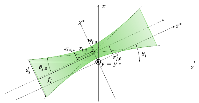
Figure 6: Drifted geometry and parameters for a focused laser pulse with incident angle $\theta_{j}$. The laser-beam coordinate system rotated by $\theta_{j}$ is denoted with the asterisk symbol. A laser pulse propagates along the dashed arrow parallel to the $z^{*}$-axis with a displacement of $\bm{r}^{*}_{j,0}$ from that in the $x^{*}-y^{*}$ plane. The focusing angle between the dashed arrow and the dash-dotted line based on geometric optics is expressed as $\vartheta_{j,0}=\tan^{-1}\left(d_{j}/2f_{j}\right)$ using diameter $d_{j}$ and focal length $f_{j}$ of beam $j$. The beam radius at the focal point is referred to as beam waist $w_{j,0}$, and the beam radius along the $z^{*}$-axis is expressed as $w_{j}$. When $w_{j}=\sqrt{2}w_{j,0}$, the distance from the focal point corresponds to Rayleigh length $z_{j,R}$.

The normalized number density distribution $\rho_{j}$ is then generalized by substituting Eq.(25) and Eq.(27) to $\rho_{j}(t_{j},\bm{r}^{*})$ as follows

$$\begin{split}&\rho_{j}(t,\bm{r}\,;\ \lambda_{j},\tau_{j},d_{j},f_{j},\theta_{j},t_{j,0},\bm{r}^{*}_{j,0})\\ &\quad=\left(\frac{2}{\pi}\right)^{\frac{3}{2}}\frac{1}{w_{j}^{2}(c_{0}t_{j})c_{0}\tau_{j}}\exp\left[-2\frac{(x\cos\theta_{j}-z\sin\theta_{j}-x^{*}_{j,0})^{2}+(y-y^{*}_{j,0})^{2}}{w_{j}^{2}(c_{0}t_{j})}\right]\\ &\qquad\exp\left[-2\left(\frac{x\sin\theta_{j}+z\cos\theta_{j}-c_{0}t_{j}}{c_{0}\tau_{j}}\right)^{2}\right].\end{split}$$ (28)

Hereinafter we abbreviate

$$w_{j}=w_{j}(c_{0}t_{j}).$$ (29)

The volume of an inducing pulse $V_{4}$ for the normalization is a quantity which is independent of the space-time coordinates and obtained by spatial integration of the squared field strength of the inducing laser pulse Yariv ; PTEP2017 ,

$$V_{4}=\left(\frac{\pi}{2}\right)^{\frac{3}{2}}w_{4,0}^{2}c_{0}\tau_{4}.$$ (30)

Substituting the space-time distributions $\rho_{j}(t,\bm{r})$ into Eq.(22), we obtain

$$\begin{split}\mathcal{D}_{exp}&=V_{4}\left(\frac{2}{\pi}\right)^{\frac{9}{2}}\int_{-z_{4,R}/c_{0}}^{0}dt\left(\prod_{j}\frac{1}{w_{j}^{2}c_{0}\tau_{j}}\right)\int_{-\infty}^{\infty}dx\int_{-\infty}^{\infty}dy\int_{-\infty}^{\infty}dz\\ &\quad\exp\left[-2\sum_{j}\left\{\left(\frac{x\cos\theta_{j}-z\sin\theta_{j}-x^{*}_{j,0}}{w_{j}}\right)^{2}+\left(\frac{y-y^{*}_{j,0}}{w_{j}}\right)^{2}+\left(\frac{x\sin\theta_{j}+z\cos\theta_{j}-c_{0}t_{j}}{c_{0}\tau_{j}}\right)^{2}\right\}\right].\end{split}$$ (31)

In the following, first, all the spatial integrations will be performed. The operation that is most frequently repeated is a re-square-completion of several square-completed quadratic functions. The sum over $j$ of square-completed quadratic functions expressed in one variable $x$ can be transformable into a single square-completed quadratic function as follows

$$\sum_{j}a_{j}(x-b_{j})^{2}=\left(\sum_{j}a_{j}\right)\left\{x-\frac{\sum_{j}a_{j}b_{j}}{\sum_{j}a_{j}}\right\}^{2}+\frac{\sum_{j,k,j<k}a_{j}a_{k}(b_{j}-b_{k})^{2}}{\sum_{j}a_{j}}$$ (32)

The summation contained in the numerator of the last term in the RHS of Eq.(32) is over $(j,k)=(1,2),(1,4),(2,4)$. Since the summed function which consists of squares of anti-symmetric elements holds $(j,k)=(k,j)$ with respect to the index combinations as in the LHS of Eq.(Appendix: Derivation for experimentally tuned density overlapping factor, $\mathcal{D}_{exp}$), this function can be regarded as a summation over $j,k$ following the cyclic order of $\{1,2,4\}$

$$\sum_{j,k,j<k}(c_{j}d_{k}-c_{k}d_{j})^{2} =\sum_{j,k=(1,2),(1,4),(2,4)}(c_{j}d_{k}-c_{k}d_{j})^{2}$$

$$=\sum_{j,k=(2,4),(4,1),(1,2)}(c_{j}d_{k}-c_{k}d_{j})^{2}$$

$$=\sum_{j}\left(\sum_{k,l}\varepsilon_{jkl}c_{k}d_{l}\right)^{2}.$$ (33)

Hereafter, the cyclic summation over $j$ and $k$ is abbreviated using the exceptional three-dimensional anti-symmetric symbol $\varepsilon_{jkl}$, which takes the sign of cyclic and anti-cyclic permutations of $\{1,2,4\}$, as follows

$$\varepsilon_{jkl}=\begin{cases}1&(j,k,l)=(1,2,4),(2,4,1),(4,1,2)\\ -1&(j,k,l)=(1,4,2),(4,2,1),(2,1,4)\\ 0&\text{otherwise}.\end{cases}$$ (34)

First, the $y$-integration in Eq.(31) is performed. In the exponent of the integrand, the $y$-dependent terms are only the second terms. The sum over $j$ of these terms can be combined into a single quadratic function by using Eq.(32) and Eq.(Appendix: Derivation for experimentally tuned density overlapping factor, $\mathcal{D}_{exp}$),

$$\sum_{j}\frac{1}{w_{j}^{2}}\left(y-y^{*}_{j,0}\right)^{2}=\left(\sum_{j}w_{j}^{-2}\right)\left(y-\frac{\sum_{j}w_{j}^{-2}y^{*}_{j,0}}{\sum_{j}w_{j}^{-2}}\right)^{2}+\sum_{j}\eta_{j}^{2},$$ (35)

where $\eta_{j}$ is defined as

$$\eta_{j}=\frac{1}{\sqrt{\sum_{m}w_{m}^{-2}}}\sum_{k,l}\varepsilon_{jkl}w_{k}^{-1}w_{l}^{-1}y^{*}_{k,0}.$$ (36)

The $y$-integral of the exponential term with Eq.(35) can be immediately perfomed as follows

$$\int_{-\infty}^{\infty}dy\exp\left[-2\sum_{j}\frac{1}{w_{j}^{2}}\left(y-y^{*}_{j,0}\right)^{2}\right]=\sqrt{\frac{\pi}{2}}\left(\sum_{j}w_{j}^{-2}\right)^{-\frac{1}{2}}\exp\left[-2\sum_{j}\eta_{j}^{2}\right].$$ (37)

Next, we turn our attention to the $x$-integral in Eq.(31). All the terms that persist after the $y$-integral exhibit the negative quadratic behavior with respect to $x$ within the exponential function, and the range of $x$-integral spans from $-\infty$ to $\infty$. Consequently, we can consolidate the coefficients of all the terms dependent on $x$ by completing the square for $x$, facilitating the subsequent integral with respect to $x$. We bundle the first and third terms in the curly bracket in Eq.(31) with individual coefficients of $x$, respectively, as follows

$$\begin{split}&\left(\frac{x\cos\theta_{j}-z\sin\theta_{j}-x^{*}_{j,0}}{w_{j}}\right)^{2}+\left(\frac{x\sin\theta_{j}+z\cos\theta_{j}-c_{0}t_{j}}{c_{0}\tau_{j}}\right)^{2}\\ &=\left(\frac{\cos\theta_{j}}{w_{j}}\right)^{2}\left(x-z\tan\theta_{j}-x^{*}_{j,0}\sec\theta_{j}\right)^{2}+\left(\frac{\sin\theta_{j}}{c_{0}\tau_{j}}\right)^{2}\left(x+z\cot\theta_{j}-c_{0}t_{j}\csc\theta_{j}\right)^{2}.\end{split}$$ (38)

Hereinafter, we define $\alpha_{j}$ and $\beta_{j}$ as

$$\alpha_{j}=\frac{1}{w_{j}^{2}}\cos\theta_{j},\qquad\beta_{j}=\frac{1}{c_{0}^{2}\tau_{j}^{2}}\sin\theta_{j}.$$ (39)

Furthermore, we temporarily replace for the sake of simplification,

$$A_{j}=\alpha_{j}\cos\theta_{j},\quad B_{j}=z\tan\theta_{j}+x^{*}_{j,0}\sec\theta_{j},\quad C_{j}=\beta_{j}\sin\theta_{j},\quad D_{j}=z\cot\theta_{j}-c_{0}t_{j}\csc\theta_{j}.$$ (40)

Equation (LABEL:eq:[th-df]:dfm_expterms) can be transformable into the re-completed square for $x$ as follows,

$$A_{j}\left(x-B_{j}\right)^{2}+C_{j}\left(x+D_{j}\right)^{2}$$

$$=\left(A_{j}+C_{j}\right)\left\{x-\frac{1}{A_{j}+C_{j}}\left(A_{j}B_{j}-C_{j}D_{j}\right)\right\}^{2}+\frac{1}{A_{j}+C_{j}}\frac{1}{\left(w_{j}c_{0}\tau_{j}\right)^{2}}\left(z+x^{*}_{j,0}\sin\theta_{j}-c_{0}t_{j}\cos\theta_{j}\right)^{2}$$

$$=\delta_{j}\left(x-E_{j}\right)^{2}+\frac{1}{\delta_{j}}\frac{1}{\left(w_{j}c_{0}\tau_{j}\right)^{2}}\left(z+F_{j}\right)^{2},$$ (41)

where $\delta_{j}$, $E_{j}$ and $F_{j}$ are defined as

$$\delta_{j} =A_{j}+C_{j}=\alpha_{j}\cos\theta_{j}+\beta_{j}\sin\theta_{j},$$ (42)

$$E_{j} =\frac{1}{\delta_{j}}\left(A_{j}B_{j}-C_{j}D_{j}\right)$$

$$=\frac{1}{\delta_{j}}\left(\left(\alpha_{j}\sin\theta_{j}-\beta_{j}\cos\theta_{j}\right)z+\alpha_{j}x^{*}_{j,0}+\beta_{j}c_{0}t_{j}\right),$$ (43)

$$F_{j} =x^{*}_{j,0}\sin\theta_{j}-c_{0}t_{j}\cos\theta_{j}.$$ (44)

$\delta_{j}$ is always positive for Eq.(39). The sum over $j$ of the last term in Eq.(Appendix: Derivation for experimentally tuned density overlapping factor, $\mathcal{D}_{exp}$) is calculated by using Eq.(32) and Eq.(Appendix: Derivation for experimentally tuned density overlapping factor, $\mathcal{D}_{exp}$) as follows

$$\begin{split}&\sum_{j}\left\{\delta_{j}\left(x-E_{j}\right)^{2}+\frac{1}{\delta_{j}}\frac{1}{\left(w_{j}c_{0}\tau_{j}\right)^{2}}\left(z+F_{j}\right)^{2}\right\}\\ &=\left(\sum_{j}\delta_{j}\right)\left(x-\frac{\sum_{j}\delta_{j}E_{j}}{\sum_{j}\delta_{j}}\right)^{2}+\frac{\sum_{j}\left(\sum_{k,l}\varepsilon_{jkl}\sqrt{\delta_{k}\delta_{l}}E_{k}\right)^{2}}{\sum_{j}\delta_{j}}+\sum_{j}\frac{1}{\delta_{j}}\frac{1}{\left(w_{j}c_{0}\tau_{j}\right)^{2}}\left(z+F_{j}\right)^{2}.\end{split}$$ (45)

We substitute Eq.(LABEL:eq:[th-df]:pfm_x_sqcpl2) into the exponential term in Eq.(31) and calculate the $x$-integration as follows

$$\int_{-\infty}^{\infty}dx\exp\left[-2\sum_{j}\left\{\delta_{j}\left(x-E_{j}\right)^{2}+\frac{1}{\delta_{j}}\frac{1}{\left(w_{j}c_{0}\tau_{j}\right)^{2}}\left(z+F_{j}\right)^{2}\right\}\right]$$

$$=\sqrt{\frac{\pi}{2}}\left(\sum_{j}\delta_{j}\right)^{-\frac{1}{2}}\exp\left[-2\left\{\frac{\sum_{j}\left(\sum_{k,l}\varepsilon_{jkl}\sqrt{\delta_{k}\delta_{l}}E_{k}\right)^{2}}{\sum_{j}\delta_{j}}+\sum_{j}\frac{1}{\delta_{j}}\frac{1}{\left(w_{j}c_{0}\tau_{j}\right)^{2}}\left(z+F_{j}\right)^{2}\right\}\right].$$ (46)

We then perform the $z$-integral. The term that depends on $z$ is only the exponential term in the RHS of Eq.(Appendix: Derivation for experimentally tuned density overlapping factor, $\mathcal{D}_{exp}$). The $z$-dependent terms, like the $x$-dependent terms, are all negative quadratic within the exponential, and the integral range is from $-\infty$ to $\infty$. Therefore, the plan is that all the terms are summarized by the square completion for $z$ and the gaussian integral of them is performed. The first term in the curly bracket in Eq.(Appendix: Derivation for experimentally tuned density overlapping factor, $\mathcal{D}_{exp}$) is square-completed at first. We transform $\sum_{k,l}\varepsilon_{jkl}\sqrt{\delta_{k}\delta_{l}}E_{k}$ to the expression that denotes $z$ explicitly as follows

$$\sum_{k,l}\varepsilon_{jkl}\sqrt{\delta_{k}\delta_{l}}E_{k} =\sqrt{\sum_{m}\delta_{m}}\left\{\frac{1}{\sqrt{\sum_{m}\delta_{m}}}\sum_{k,l}\varepsilon_{jkl}\sqrt{\frac{\delta_{l}}{\delta_{k}}}\left(\alpha_{k}\sin\theta_{k}-\beta_{k}\cos\theta_{k}\right)z\right.$$ (47)

$$\qquad\left.+\frac{1}{\sqrt{\sum_{m}\delta_{m}}}\sum_{k,l}\varepsilon_{jkl}\sqrt{\frac{\delta_{l}}{\delta_{k}}}\left(\alpha_{k}x^{*}_{k,0}+\beta_{k}c_{0}t_{k}\right)\right\}$$

$$=\sqrt{\sum_{m}\delta_{m}}\left(\mu_{j}z+\xi_{j}\right),$$ (48)

where $\mu_{j}$ and $\xi_{j}$ are defined as

$$\begin{split}\mu_{j}&=\frac{1}{\sqrt{\sum_{m}\delta_{m}}}\sum_{k,l}\varepsilon_{jkl}\sqrt{\frac{\delta_{l}}{\delta_{k}}}\left(\alpha_{k}\sin\theta_{k}-\beta_{k}\cos\theta_{k}\right),\qquad\\[4.0pt] \xi_{j}&=\frac{1}{\sqrt{\sum_{m}\delta_{m}}}\sum_{k,l}\varepsilon_{jkl}\sqrt{\frac{\delta_{l}}{\delta_{k}}}\left(\alpha_{k}x^{*}_{k,0}+\beta_{k}c_{0}t_{k}\right).\end{split}$$ (49)

The first term in the curly bracket in the exponential function in Eq.(Appendix: Derivation for experimentally tuned density overlapping factor, $\mathcal{D}_{exp}$) can be square-completed using Eq.(32) and Eq.(Appendix: Derivation for experimentally tuned density overlapping factor, $\mathcal{D}_{exp}$)

$$\frac{1}{\sum_{j}\delta_{j}}\sum_{j}\left(\sum_{k,l}\varepsilon_{jkl}\sqrt{\delta_{k}\delta_{l}}E_{k}\right)^{2} =\sum_{j}\mu_{j}^{2}\left(z+\frac{\xi_{j}}{\mu_{j}}\right)^{2}$$

$$=\left(\sum_{j}\mu_{j}^{2}\right)\left(z+\frac{\sum_{j}\mu_{j}\xi_{j}}{\sum_{j}\mu_{j}^{2}}\right)^{2}+\frac{\sum_{j}\left(\sum_{k,l}\varepsilon_{jkl}\mu_{j}\xi_{k}\right)^{2}}{\sum_{j}\mu_{j}^{2}}.$$ (50)

The second term is also the sum of quadratic functions for $z$ distinguished by the subscript $j$, which is then square-completed to the single quadratic function with respect to $z$ using Eq.(32) as follows

$$\sum_{j}\frac{1}{\delta_{j}}\frac{1}{\left(w_{j}c_{0}\tau_{j}\right)^{2}}\left(z+F_{j}\right)^{2} =\sum_{j}\left(\frac{1}{w_{j}c_{0}\tau_{j}\sqrt{\delta_{j}}}z+\frac{1}{w_{j}c_{0}\tau_{j}\sqrt{\delta_{j}}}\left(x^{*}_{j,0}\sin\theta_{j}-c_{0}t_{j}\cos\theta_{j}\right)\right)^{2}$$

$$=\sum_{j}\left(\nu_{j}z+\zeta_{j}\right)^{2}$$

$$=\left(\sum_{j}\nu_{j}^{2}\right)\left(z+\frac{\sum_{j}\nu_{j}\zeta_{j}}{\sum_{j}\nu_{j}^{2}}\right)^{2}+\frac{\sum_{j}\left(\sum_{k,l}\varepsilon_{jkl}\nu_{k}\zeta_{l}\right)^{2}}{\sum_{j}\nu_{j}^{2}},$$ (51)

where

$$\begin{split}\nu_{j}=\frac{1}{w_{j}c_{0}\tau_{j}\sqrt{\delta_{j}}},\qquad\zeta_{j}=\frac{1}{w_{j}c_{0}\tau_{j}\sqrt{\delta_{j}}}\left(x^{*}_{j,0}\sin\theta_{j}-c_{0}t_{j}\cos\theta_{j}\right).\end{split}$$ (52)

The terms depending on $z$ enumerated in Eq.(Appendix: Derivation for experimentally tuned density overlapping factor, $\mathcal{D}_{exp}$) leave the two terms after the respective formula transformations: the individual first terms in the second lines of the RHS in Eq.(Appendix: Derivation for experimentally tuned density overlapping factor, $\mathcal{D}_{exp}$) and Eq.(Appendix: Derivation for experimentally tuned density overlapping factor, $\mathcal{D}_{exp}$). They are further square-completed as follows

$$\begin{split}&\left(\sum_{j}\mu_{j}^{2}\right)\left(z+\frac{\sum_{j}\mu_{j}\xi_{j}}{\sum_{j}\mu_{j}^{2}}\right)^{2}+\left(\sum_{j}\nu_{j}^{2}\right)\left(z+\frac{\sum_{j}\nu_{j}\zeta_{j}}{\sum_{j}\nu_{j}^{2}}\right)^{2}\\ &=\left(\sum_{j}\left(\mu_{j}^{2}+\nu_{j}^{2}\right)\right)\left(z+\frac{\sum_{j}\left(\mu_{j}\xi_{j}+\nu_{j}\zeta_{j}\right)}{\sum_{j}\left(\mu_{j}^{2}+\nu_{j}^{2}\right)}\right)^{2}+\frac{\left(\sum_{j}\mu_{j}^{2}\right)\left(\sum_{j}\nu_{j}^{2}\right)}{\sum_{j}\mu_{j}^{2}+\sum_{j}\nu_{j}^{2}}\left(\frac{\sum_{j}\mu_{j}\xi_{j}}{\sum_{j}\mu_{j}^{2}}-\frac{\sum_{j}\nu_{j}\zeta_{j}}{\sum_{j}\nu_{j}^{2}}\right)^{2}.\end{split}$$ (53)

Then, the first term in Eq.(LABEL:eq:[th-df]:pfm_z_sqcpl3) can be $z$-integrated

$$\begin{split}&\int_{-\infty}^{\infty}dz\exp\left[-2\left(\sum_{j}\left(\mu_{j}^{2}+\nu_{j}^{2}\right)\right)\left(z+\frac{\sum_{j}\mu_{j}\xi_{j}+\sum_{j}\nu_{j}\zeta_{j}}{\sum_{j}\left(\mu_{j}^{2}+\nu_{j}^{2}\right)}\right)^{2}\right]\\ &\quad=\sqrt{\frac{\pi}{2}}\left(\sum_{j}\left(\mu_{j}^{2}+\nu_{j}^{2}\right)\right)^{-\frac{1}{2}}.\end{split}$$ (54)

All the spatial integrations are now completed. Based on Eq.(31), the terms obtained by integrations are simply enumerated in the product form as shown in Eq.(55). In total, there are two major terms by the spatial integrations: (I) the result from the $y$-integration in Eq.(37), (II) the results from the $x$- and $z$-integrations in Eq.(Appendix: Derivation for experimentally tuned density overlapping factor, $\mathcal{D}_{exp}$) and Eq.(LABEL:eq:[th-df]:pfm_z_int) and three residual terms due to re-square-completions with respect to $z$ in Eq.(Appendix: Derivation for experimentally tuned density overlapping factor, $\mathcal{D}_{exp}$), Eq.(Appendix: Derivation for experimentally tuned density overlapping factor, $\mathcal{D}_{exp}$) and Eq.(LABEL:eq:[th-df]:pfm_z_sqcpl3).

$$\begin{split}\mathcal{D}_{exp}&=V_{4}\left(\frac{2}{\pi}\right)^{\frac{9}{2}}\int_{-z_{4,R}/c_{0}}^{0}dt\left(\prod_{j}\frac{1}{w_{j}^{2}c_{0}\tau_{j}}\right)\times\sqrt{\frac{\pi}{2}}\left(\sum_{j}w_{j}^{-2}\right)^{-\frac{1}{2}}\exp\left[-2\sum_{j}\eta_{j}^{2}\right]\\ &\qquad\times\sqrt{\frac{\pi}{2}}\left(\sum_{j}\delta_{j}\right)^{-\frac{1}{2}}\sqrt{\frac{\pi}{2}}\left(\sum_{j}\left(\mu_{j}^{2}+\nu_{j}^{2}\right)\right)^{-\frac{1}{2}}\exp\left[-2\frac{\sum_{j}\left(\sum_{k,l}\varepsilon_{jkl}\mu_{k}\xi_{l}\right)^{2}}{\sum_{j}\mu_{j}^{2}}\right]\\ &\qquad\quad\exp\left[-2\frac{\sum_{j}\left(\sum_{k,l}\varepsilon_{jkl}\nu_{k}\zeta_{l}\right)^{2}}{\sum_{j}\nu_{j}^{2}}\right]\exp\left[-2\frac{\left(\sum_{j}\mu_{j}^{2}\right)\left(\sum_{j}\nu_{j}^{2}\right)}{\sum_{j}\left(\mu_{j}^{2}+\nu_{j}^{2}\right)}\left(\frac{\sum_{j}\mu_{j}\xi_{j}}{\sum_{j}\mu_{j}^{2}}-\frac{\sum_{j}\nu_{j}\zeta_{j}}{\sum_{j}\nu_{j}^{2}}\right)^{2}\right].\end{split}$$ (55)

The numerators of the two of the last three exponential terms can be simplified as

$$\sum_{j}\left(\sum_{k,l}\varepsilon_{jkl}\mu_{k}\xi_{l}\right)^{2} =\left(\sum_{j}\mu_{j}^{2}\right)\left(\sum_{j}\xi_{j}^{2}\right)-\left(\sum_{j}\mu_{j}\xi_{j}\right)^{2},$$ (56a)

$$\sum_{j}\left(\sum_{k,l}\varepsilon_{jkl}\nu_{k}\zeta_{l}\right)^{2} =\left(\sum_{j}\nu_{j}^{2}\right)\left(\sum_{j}\zeta_{j}^{2}\right)-\left(\sum_{j}\nu_{j}\zeta_{j}\right)^{2}.$$ (56b)

Finally, the experimental $\cal{D}$-factor is derived as

$$\begin{split}\mathcal{D}_{exp}&=\left(\frac{2}{\pi}\right)^{\frac{3}{2}}w_{4,0}^{2}c_{0}\tau_{4}\int_{-z_{4,\mathit{R}}/c_{0}}^{0}dt\frac{1}{\sqrt{\left(\sum_{j}w_{j}^{-2}\right)\left(\sum_{j}\delta_{j}\right)\left(\sum_{j}\left(\mu_{j}^{2}+\nu_{j}^{2}\right)\right)}}\\ &\qquad\left(\prod_{j}\frac{1}{w_{j}^{2}c_{0}\tau_{j}}\right)\exp\left[-2\left\{\sum_{j}\left(\xi_{j}^{2}+\eta_{j}^{2}+\zeta_{j}^{2}\right)-\frac{\left(\sum_{j}\left(\mu_{j}\xi_{j}+\nu_{j}\zeta_{j}\right)\right)^{2}}{\sum_{j}\left(\mu_{j}^{2}+\nu_{j}^{2}\right)}\right\}\right].\end{split}$$ (57)

Since there is the complicated time-dependent exponential term, the analytical time integration over the finite integral range is not practical. The parameters used in Eq.(57) ( $\alpha_{j},\beta_{j}$ in Eq.(39); $\delta_{j}$ in Eq.(42); $\mu_{j},\xi_{j}$ in Eq.(49); $\nu_{j},\zeta_{j}$ in Eq.(52); $\eta_{j}$ in Eq.(36) ) are summarized in the following set of parameters

$$\alpha_{j} =\frac{1}{w_{j}^{2}}\cos\theta_{j},\qquad\beta_{j}=\frac{1}{c_{0}^{2}\tau_{j}^{2}}\sin\theta_{j},\qquad\delta_{j}=\alpha_{j}\cos\theta_{j}+\beta_{j}\sin\theta_{j},\hskip 120.0pt$$ (58)

$$\mu_{j} =\frac{1}{\sqrt{\sum_{m}\delta_{m}}}\sum_{k,l}\varepsilon_{jkl}\sqrt{\frac{\delta_{l}}{\delta_{k}}}\left(\alpha_{k}\sin\theta_{k}-\beta_{k}\cos\theta_{k}\right),\qquad\nu_{j}=\frac{1}{w_{j}c_{0}\tau_{j}\sqrt{\delta_{j}}},$$

$$\xi_{j} =\frac{1}{\sqrt{\sum_{m}\delta_{m}}}\sum_{k,l}\varepsilon_{jkl}\sqrt{\frac{\delta_{l}}{\delta_{k}}}\left(\alpha_{k}x^{*}_{k,0}+\beta_{k}c_{0}t_{k}\right),\qquad\eta_{j}=\frac{1}{\sqrt{\sum_{m}w_{m}^{-2}}}\sum_{k,l}\varepsilon_{jkl}w_{k}^{-1}w_{l}^{-1}y^{*}_{k,0},$$

$$\zeta_{j} =\frac{1}{w_{j}c_{0}\tau_{j}\sqrt{\delta_{j}}}\left(x^{*}_{j,0}\sin\theta_{j}-c_{0}t_{j}\cos\theta_{j}\right).$$

The parameters $\xi_{j},\eta_{j},\zeta_{j}$ are caused by the drifts of propagation directions of individual pulses in the $x^{*}-y^{*}$ plane, $x^{*}_{j,0},y^{*}_{j,0}$. Especially, both $\xi_{j}$ and $\zeta_{j}$ explicitly include $x^{*}_{j,0}$ and $c_{0}t_{j}$ since $x$ and $z$ components are correlated by rotations of laser pulse propagation directions in the $z-x$ plane.

When the focused spacetime points of individual pulses reach the oring, the temporal drift becomes $t_{j,0}=0$ and the spatial drifts $x^{*}_{j,0}=y^{*}_{j,0}=0$ are satisfied. The parameters for ${\cal{D}}_{exp}$ in such an ideal case are thus summarized as

$$\alpha_{j} =\frac{1}{w_{j}^{2}}\cos\theta_{j},\qquad\beta_{j}=\frac{1}{c_{0}^{2}\tau_{j}^{2}}\sin\theta_{j},\qquad\delta_{j}=\alpha_{j}\cos\theta_{j}+\beta_{j}\sin\theta_{j},\hskip 120.0pt$$ (59)

$$\mu_{j} =\frac{1}{\sqrt{\sum_{m}\delta_{m}}}\sum_{k,l}\varepsilon_{jkl}\sqrt{\frac{\delta_{l}}{\delta_{k}}}\left(\alpha_{k}\sin\theta_{k}-\beta_{k}\cos\theta_{k}\right),\qquad\nu_{j}=\frac{1}{w_{j}c_{0}\tau_{j}\sqrt{\delta_{j}}},$$

$$\xi_{j} =\frac{1}{\sqrt{\sum_{m}\delta_{m}}}\sum_{k,l}\varepsilon_{jkl}\sqrt{\frac{\delta_{l}}{\delta_{k}}}\beta_{k}c_{0}t,\qquad\eta_{j}=0,\qquad\zeta_{j}=-\frac{1}{w_{j}c_{0}\tau_{j}\sqrt{\delta_{j}}}c_{0}t\cos\theta_{j}.$$

In order to cross-check the complicated formulae for ${\cal{D}}_{exp}$, we compare the $\cal{D}$-factor, ${\cal{D}}_{c+i}$, applied to a quasi-parallel collision system (QPS) consisting of two beams, creation beam ($c$) and inducing beam ($i$), which is the simplest and practical collisional system dedicated for SRPC SAPPHIRES00 . In QPS, creation photons are arbitrarily selected from a single common pulse laser resulting in an ALP creation. Since creation and inducing laser pulses co-axially propagate in QPS and are focused by an off-axis parabolic mirror, these incident angles are $\theta_{j}=0$. The corresponding parameters in Eq.(58) are then as follows

$$\alpha_{j} =\frac{1}{w_{j}^{2}},\qquad\beta_{j}=0,\qquad\delta_{j}=\frac{1}{w_{j}^{2}},\qquad\mu_{j}=0,\qquad\nu_{j}=\frac{1}{c_{0}\tau_{j}},\hskip 132.0pt$$ (60)

$$\xi_{j} =\frac{1}{\sqrt{\sum_{m}w_{m}^{-2}}}\sum_{k,l}\varepsilon_{jkl}w_{k}^{-1}w_{l}^{-1}x^{*}_{k,0},\quad\eta_{j}=\frac{1}{\sqrt{\sum_{m}w_{m}^{-2}}}\sum_{k,l}\varepsilon_{jkl}w_{k}^{-1}w_{l}^{-1}y^{*}_{k,0},\quad\zeta_{j}=-\frac{t_{j}}{\tau_{j}}.$$

For the sake of clarity, we introduce notations for QPS as follows $w_{c}\equiv w_{1}=w_{2}$ and $w_{i}\equiv w_{4}$, $\tau_{c}\equiv\tau_{1}=\tau_{2}$ and $\tau_{i}\equiv\tau_{4}$. The $\cal{D}$-factor in QPS, $\mathcal{D}_{c+i}^{Q}$, is transformed by substituting the parameters in Eq.(60) into Eq.(57) as follows

$$\mathcal{D}_{c+i}^{Q} =\left(\frac{2}{\pi}\right)^{\frac{3}{2}}\frac{1}{c_{0}}\frac{\tau_{i}}{\tau_{c}}\frac{1}{\sqrt{\tau_{c}^{2}+2\tau_{i}^{2}}}w_{i,0}^{2}\int_{-z_{i,R}/c_{0}}^{0}dt\frac{1}{w_{c}^{2}\left(w_{c}^{2}+2w_{i}^{2}\right)}\exp\left[-2\sum_{j}\left(\xi_{j}^{2}+\eta_{j}^{2}\right)\right].$$ (61)

The exponential term in Eq.(61) expresses the deviations between the profiles of two laser pulses at the focal point as

$$\sum_{j}\left(\xi_{j}^{2}+\eta_{j}^{2}\right)=\frac{2}{w_{c}^{2}+2w_{i}^{2}}\left\{\left(x^{*}_{c,0}-x^{*}_{i,0}\right)^{2}+\left(y^{*}_{c,0}-y^{*}_{i,0}\right)^{2}\right\}.$$ (62)

As the ideal situation in QPS, we consider the case where time drift $t_{j,0}$ and spatial drift $x^{*}_{j,0},y^{*}_{j,0}$ are absent. Since Eq.(62) becomes null, Eq.(61) is expressed as

$$\mathcal{D}_{c+i}^{Q}=\left(\frac{2}{\pi}\right)^{\frac{3}{2}}\frac{1}{c_{0}}\frac{\tau_{i}}{\tau_{c}}\frac{1}{\sqrt{\tau_{c}^{2}+2\tau_{i}^{2}}}w_{i,0}^{2}\int_{-z_{i,R}/c_{0}}^{0}dt\frac{1}{w_{c}^{2}(c_{0}t)\left(w_{c}^{2}(c_{0}t)+2w_{i}^{2}(c_{0}t)\right)},$$ (63)

where

$$\frac{1}{w_{c}^{2}(c_{0}t)\left(w_{c}^{2}(c_{0}t)+2w_{i}^{2}(c_{0}t)\right)}=\frac{1}{2\left(w_{c,0}^{2}\vartheta_{i,0}^{2}-w_{i,0}^{2}\vartheta_{c,0}^{2}\right)}\left[\frac{\vartheta_{c,0}^{2}}{w_{c}^{2}(c_{0}t)}-\frac{\vartheta_{c,0}^{2}+2\vartheta_{i,0}^{2}}{w_{c}^{2}(c_{0}t)+2w_{i}^{2}(c_{0}t)}\right].$$ (64)

Eventually, $\mathcal{D}_{c+i}^{Q}$ is thus simplified as

$$\mathcal{D}_{c+i}^{Q}=\sqrt{\frac{2}{\pi^{3}}}\frac{1}{c_{0}^{2}}\frac{\tau_{i}}{\tau_{c}}\frac{1}{\sqrt{\tau_{c}^{2}+2\tau_{i}^{2}}}\frac{1}{\vartheta_{c,0}^{2}\left(1-\frac{z_{c,R}^{2}}{z_{i,R}^{2}}\right)}\left[\frac{1}{z_{c,R}}\tan^{-1}\left(\frac{z_{i,R}}{z_{c,R}}\right)-\frac{1}{Z_{ci}}\tan^{-1}\left(\frac{z_{i,R}}{Z_{ci}}\right)\right]$$ (65)

with

$$Z_{ci}\equiv\sqrt{\frac{w_{c,0}^{2}+2w_{i,0}^{2}}{\vartheta_{c,0}^{2}+2\vartheta_{i,0}^{2}}}.$$ (66)

This expression exactly coincides with that in the published paper SAPPHIRES00 , which is derived starting from the idealized QPS case.

References

• (1) R. D. Peccei and H. R. Quinn, Phys. Rev. Lett 38, 1440 (1977)
• (2) S. Weinberg, Phys. Rev. Lett 40, 223 (1978); F. Wilczek, Phys. Rev. Lett 40, 271 (1978); J. E. Kim, Phys. Rev. Lett. 43, 103 (1979); M. A. Shifman, A. I. Vainshtein and V. I. Zakharov, Nucl. Phys. B 166, 493 (1980).
• (3) J. Preskill, M. B. Wise and F. Wilczek, “Cosmology of the Invisible Axion,” Phys. Lett. B 120, 127-132 (1983) doi:10.1016/0370-2693(83)90637-8
• (4) L. F. Abbott and P. Sikivie, “A Cosmological Bound on the Invisible Axion,” Phys. Lett. B 120, 133-136 (1983) doi:10.1016/0370-2693(83)90638-X
• (5) M. Dine and W. Fischler, “The Not So Harmless Axion,” Phys. Lett. B 120, 137-141 (1983) doi:10.1016/0370-2693(83)90639-1
• (6) S. M. Boucenna and Q. Shafi, “Axion inflation, proton decay, and leptogenesis in $SU(5)\times U(1)_{PQ}$,” Phys. Rev. D 97, no.7, 075012 (2018) doi:10.1103/PhysRevD.97.075012 [arXiv:1712.06526 [hep-ph]].
• (7) A. Ernst, A. Ringwald and C. Tamarit, “Axion Predictions in $SO(10)\times U(1)_{\rm PQ}$ Models,” JHEP 02, 103 (2018) doi:10.1007/JHEP02(2018)103 [arXiv:1801.04906 [hep-ph]].
• (8) R. Daido, F. Takahashi and W. Yin, “The ALP miracle: unified inflaton and dark matter,” JCAP 05, 044 (2017) doi:10.1088/1475-7516/2017/05/044 [arXiv:1702.03284 [hep-ph]].
• (9) R. Daido, F. Takahashi and W. Yin, “The ALP miracle revisited,” JHEP 02, 104 (2018) doi:10.1007/JHEP02(2018)104 [arXiv:1710.11107 [hep-ph]].
• (10) C. Bartram et al. [ADMX], “Search for Invisible Axion Dark Matter in the 3.3–4.2  $\mu$eV Mass Range,” Phys. Rev. Lett. 127, no.26, 261803 (2021) doi:10.1103/PhysRevLett.127.261803 [arXiv:2110.06096 [hep-ex]].
• (11) V. Anastassopoulos et al. (CAST), Nature Phys. 13, 584 (2017).
• (12) Y. Fujii and K. Homma, Prog. Theor. Phys 126, 531 (2011); Prog. Theor. Exp. Phys. 089203 (2014) [erratum].
• (13) K. Homma and Y. Kirita, “Stimulated radar collider for probing gravitationally weak coupling pseudo Nambu-Goldstone bosons,” JHEP 09, 095 (2020) doi:10.1007/JHEP09(2020)095 [arXiv:1909.00983 [hep-ex]].
• (14) K. Homma, F. Ishibashi, Y. Kirita and T. Hasada, “Sensitivity to axion-like particles with a three-beam stimulated resonant photon collider around the eV mass range,” Universe 9, 20 (2023) doi:10.3390/universe9010020 [arXiv:2212.13012 [hep-ph]].
• (15) K. Homma, T. Hasebe, and K.Kume, Prog. Theor. Exp. Phys. 083C01 (2014).
• (16) T. Hasebe, K. Homma, Y. Nakamiya, K. Matsuura, K. Otani, M. Hashida, S. Inoue, S. Sakabe, Prog. Theo. Exp. Phys. 073C01 (2015).
• (17) A. Nobuhiro, Y. Hirahara, K. Homma, Y. Kirita, T. Ozaki, Y. Nakamiya, M. Hashida, S. Inoue, and S. Sakabe, Prog. Theo. Exp. Phys. 073C01 (2020).
• (18) K. Homma, Y. Kirita, M. Hashida, Y. Hirahara, S. Inoue, F. Ishibashi, Y. Nakamiya, L. Neagu, A. Nobuhiro, T. Ozaki, M. Rosu, S. Sakabe and O. Tesileanu (SAPPHIRES), Journal of High Energy Physics, 12, (2021) 108.
• (19) Y. Kirita, T. Hasada, M. Hashida, Y. Hirahara, K. Homma, S. Inoue, F. Ishibashi, Y. Nakamiya, L. Neagu, A. Nobuhiro, T. Ozaki, M. Rosu, S. Sakabe and O. Tesileanu (SAPPHIRES), Journal of High Energy Physics, 10, (2022) 176.
• (20) F. Ishibashi, T. Hasada, K. Homma, Y. Kirita, T. Kanai, S. Masuno, S. Tokita and M. Hashida, “Pilot Search for Axion-Like Particles by a Three-Beam Stimulated Resonant Photon Collider with Short Pulse Lasers,” Universe 9, no.3, 123 (2023) doi:10.3390/universe9030123 [arXiv:2302.06016 [hep-ex]].
• (21) T. Hasada, K. Homma and Y. Kirita, “Design and Construction of a Variable-Angle Three-Beam Stimulated Resonant Photon Collider toward eV-Scale ALP Search,” Universe 9, no.8, 355 (2023) doi:10.3390/universe9080355 [arXiv:2306.06703 [hep-ex]].
• (22) http://www.cst.com/
• (23) https://eli-laser.eu
• (24) E. Li, H. Uehara, S. Tokita, M. Zhao, R. Yasuhara, “High-power, single-frequency mid-infrared laser based on a hybrid Fe:Znse amplifier,” Infrared Physics & Technology 136, 105071 (2024). https://doi.org/10.1016/j.infrared.2023.105071; A. V. Pushkin, E. A. Migal, S. Tokita, Yu. V. Korostelin, and F. V. Potemkin, “Femtosecond graphene mode-locked Fe:ZnSe laser at 4.4 $\mu$m,” Opt. Lett. 45, 738-741 (2020).
• (25) K. Homma, Y. Kirita and F. Ishibashi, “Perspective of Direct Search for Dark Components in the Universe with Multi-Wavelengths Stimulated Resonant Photon-Photon Colliders,” Universe 7, no.12, 479 (2021) doi:10.3390/universe7120479
• (26) J. D. Bjorken and S. D. Drell, Relativistic Quantum Mechanicsh, McGraw-Hill, Inc. (1964); See also Eq.(3.80) in W. Greiner and J. Reinhardt, Quantum Electrodynamics Second Edition, Springer (1994).
• (27) See Eq.(36.56) in J. Beringer et al. (Particle Data Group), Phys. Rev. D 86, 010001 (2012).
• (28) K. Hattori, T. Konno, Y. Miura, S. Takasu and D. Fukuda, “An optical transition-edge sensor with high energy resolution,” Supercond. Sci. Technol. 35, no.9, 095002 (2022) doi:10.1088/1361-6668/ac7e7b [arXiv:2204.01903 [physics.ins-det]].
• (29) S. H. Kim, Y. Takeuchi, T. Iida, et al., “Development of Superconducting Tunnel Junction Far-Infrared Photon Detector for Cosmic Background Neutrino Decay Search - COBAND Experiment,” PoS (ICHEP2018) 427.
• (30) J. J. A. Baselmans et al., “A kilo-pixel imaging system for future space based far-infrared observatories using microwave kinetic inductance detectors,” Astron. Astrophys 601, A89 (2017) doi:10.1051/0004-6361/201629653 [arxiv:1609.01952 [astro-ph.IM]].
• (31) P. M. Echternach et al., “Single photon detection of 1.5 THz radiation with the quantum capacitance detector,” Nat Astron 2, 90-97 (2018) doi:10.1038/s41550-017-0294-y
• (32) J. Liu et al. [BREAD], “Broadband Solenoidal Haloscope for Terahertz Axion Detection,” Phys. Rev. Lett. 128, no.13, 131801 (2022) doi:10.1103/PhysRevLett.128.131801 [arXiv:2111.12103 [physics.ins-det]].
• (33) Infrared Laboratories, Bolometers hrefhttps://www.irlabs.com/products/bolometers/Bolomters
• (34) M. L. Ridder, P. Khosropanah, R. A. Hijmering, T. Suzuki, M. P. Bruijn, H. F. C. Hoevers, J. R. Gao, and M. R. Zuiddam “Fabrication of Low-Noise TES Arrays for the SAFARI Instrument on SPICA,” J Low Temp Phys 184, 60-65 (2016) doi:10.1007/s10909-015-1381-z
• (35) P. M. Echternach, A. D. Beyer, and C. M. Bradford, “Large array of low-frequency readout quantum capacitance detectors,” J. Astron. Telesc. Instrum. Syst. 7, 1-8 (2021) doi:10.1117/1.JATIS.7.1.011003
• (36) A. Ayalaet al., Phys. Rev. Lett. 113, 19, 191302 (2014).
• (37) J. E. Kim, Phys. Rev. Lett. 43, 103 (1979); M. Shifman, A. Vainshtein, and V. Zakharov, Nucl. Phys. B166, 493 (1980).
• (38) M. Dine, W. Fischler, and M. Srednicki, Phys. Lett. 104B, 199 (1981); A. Zhitnitskii, Sov. J. Nucl. Phys. 31, 260 (1980).
• (39) K. Homma and Y. Toyota, “Exploring pseudo-Nambu–Goldstone bosons by stimulated photon colliders in the mass range 0.1 eV to 10 keV,” PTEP 2017, no.6, 063C01 (2017) doi:10.1093/ptep/ptx069 [arXiv:1701.04282 [hep-ph]].
• (40) Amnon Yariv, Optical Electronics in Modern Communications Oxford University Press (1997).