Josephson junction of minimally twisted bilayer graphene

Abstract

We theoretically investigate the transport properties of Josephson junctions composed of superconductor/minimally twisted bilayer graphene/superconductor structures. In the presence of an out-of-plane electric field, the low energy physics is best described by a network of chiral domain-wall states. Depending on system parameters, they lead to the emergence of zig-zag or pseudo-Landau level modes with distinct transport characteristics. Specifically, we find zig-zag modes feature linear dispersion of Andreev bound states, resulting in a $4\pi$-periodic Josephson current. In contrast, pseudo-Landau level modes exhibit flat Andreev bound states and, consequently, a vanishing bulk Josephson current. Interestingly, edge states can give rise to $4\pi$-periodic Josephson response in the pseudo-Landau level regime. We also discuss experimental signatures of such responses.

I Introduction

The discovery of correlated insulating states and unconventional superconductivity [1, 2] in twisted bilayer graphene has generated significant interest in moiré materials. Such systems are described by a periodic potential induced by the interference pattern of two rotationally misaligned graphene layers [3]. Moiré materials exist at the intersection of two paradigms: topological and electronic correlation physics [4, 5, 6, 7]. The coexistence of these effects promotes novel electronic phases that did not exist in each of the paradigms individually. Such as, around the magic angle of 1^∘, twisted bilayer graphene hosts flat bands, where electron correlation effects dominate, giving rise various broken symmetry phases [8, 9, 10, 11, 12, 13, 14, 15, 16, 17, 18, 19, 20, 21, 22, 23], whereas away from the magic angle, band topological properties such as the Chern number and geometric quantities such as the quantum metric may play an important role [24, 25, 26, 27].

In a minimally twisted ($\theta\ll 1^{\circ}$) bilayer graphene (MTBG), lattice relaxations become significant in TBG, leading to the formation of sharply defined triangular domains of alternating AB and BA Bernal stacked graphene [28, 29]. The size of these triangular domains are determined by the moiré length scale, $l\sim a_{0}/\theta[\text{rad}]$ ($a_{0}=2.46\,\text{\AA}$ is graphene’s lattice constant). As $l\gg a_{0}$, the number of carbon atoms within these domains are of the order of $10^{4}(\theta^{\circ})^{-2}$, making atomistic quantum transport calculations challenging. However, in the presence of an electrostatic potential bias between the layers, these domains are insulating at charge neutrality, and non-trivial valley Chern indices result in chiral domain-wall modes per spin and valley [30, 31, 32]. At small temperatures, the electronic transport properties of this system are then described by a network of such valley-Hall domain-wall modes. A Chalker-Coddington network model [33] captures the low-energy electronic physics effectively, which is demonstrated in recent transport studies in MTBG [34, 35]. This model successfully explains Aharanov-Bohm oscillations and incorporates zig-zag (ZZ) modes predicted from microscopic calculations [36, 37]. Moreover, under specific network parameters, it predicts circulating modes, termed pseudo-Landau level (pLL) modes. The network becomes transparent in the presence of zig-zag modes, whereas the pseudo-Landau level modes render it insulating. Aharanov-Bohm oscillation in the presence of a magnetic field due to such a network of domain-wall modes has also been observed recently [38, 39].

Apart from magneto-conductance, it is also important to study the transport phenomena in MTBG in other experimental settings and how they arise from and differ among zig-zag or pseudo-Landau level modes. Such a study will provide us with additional insight into the microscopic underpinnings of these systems. In this regard, we choose a superconductor-MTBG-superconductor junction, i.e., a Josephson junction. Josephson junctions have been extensively studied near the magic angel in TBG [40, 41, 42]. Carrier concentration can be tuned by electrostatic gates in these systems. With this gate control, it is possible to vary the local filling factors and have two superconducting regions separated by a non-superconducting regions within a single sample of TBG. However, Josephson junctions in MTBG remain unexplored.

In this work, we study transport in a superconductor-MTBG-superconductor junction, i.e., a Josephson junction with a finite out-of-plane electric-field. We consider the superconducting leads to be $s$-wave superconductors. For the MTBG, we adopt a phenomenological Chalker-Coddington network model from previous transport studies [34, 35]. Although the microscopic origin of the network parameters remains unknown, the merit of the network model lies in the fact that it conforms to the microscopic symmetry of MTBG. We perform a comprehensive study of Andreev bound states and Josephson current within this junction for a range of network parameters. We show that zig-zag modes yield zero-energy Andreev bound states and $4\pi$ periodic Josephson current. Conversely, the pseudo-Landau level modes host perfectly flat Andreev bound states and a vanishing Josephson current. By tuning the network parameter as we tune from zig-zag modes to the pseudo-Landau level modes, the ABS gap out by merging two Dirac cones in the momentum space. The Josephson current is $2\pi$ or $4\pi$ periodic for other network parameters. Furthermore, we study the effect of edges in the Josephson junction and find that when pseudo-Landau level modes are present, the Josephson current becomes finite and is mediated through the network’s edges only. Moreover, we examine the influence of edges on the Josephson junction and find that in the presence of pseudo-Landau level modes, the Josephson current remains finite and is mediated through the edges of the network only.

The remaining part of the paper is structured as follows: In Section II, we describe the network model and the Josephson junction; in Section III, we outline the calculation procedure for Andreev bound states and Josephson current within a bulk Josephson junction; and in Section IV, we present numerical results for the same. In Section V, we extend our analysis to investigate the effects of edges in MTBG on Andreev bound states and Josephson current. Finally, we conclude with Section VI.

II Josephson junction

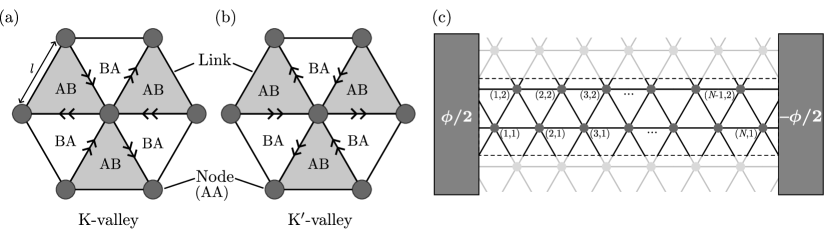
Figure 1: Schematic representation of minimally twisted bilayer graphene (MTBG) for (a) K and (b) K^′-valley. The gray and white triangles denote AB and BA stacked regions of graphene, respectively. Their boundaries host two valley-Hall states per valley and spin. The velocity of these states are opposite for K and K^′-valleys. The dark circles represent the scattering nodes consisting of AA stacked regions. (c) shows the geometry considered here for the Josephson junction, composed of two $s$-wave spin singlet superconducting leads (gray rectangles) connected by MTBG. Nodes are indexed by two integers $(m,n)$, which are connected by network links (black lines). We assume a periodic boundary condition in the transverse direction. The dashed lines encapsulate the unit-cell of the network.

We consider a Josephson junction (JJ) composed of two $s$-wave superconducting leads sandwiched by the MTBG. Superconducting order parameters for the left and right leads are $\Delta e^{\pm i\phi/2}$, respectively. In this context, $\Delta$ represents the superconducting gap, while $\phi$ refers to the phase. We describe the MTBG utilising a phenomenological network model [34, 43, 44, 35], which is an effective description of two minimally twisted ($\theta\ll 1^{\circ}$) layers of graphene in the presence of an out-of-plane electric field. For such small twist-angles, lattice relaxation leads to the formation of triangular domains of AB and BA stacked graphene of moiré length scale $l=a_{0}/\theta[\text{rad}]$. Fig. 1 (a) and (b) depict the schematic diagram of the triangular domains of AB and BA bilayer graphene for the K and K^′ valleys, respectively. In the presence of an electrostatic potential ($U$), the energy spectrum of the bulk of the domains become gapped, leaving ballistic domain-wall (DW) modes on the domain boundaries. There are two DW modes per valley per spin, as the change of valley-Chern number across the AB and BA domain is $\Delta C_{\text{v}}=\pm 2\,\mathrm{sgn}(U/t_{\perp})$ [31, 32, 45], where $\pm$ stands for AB and BA domains respectively and $t_{\perp}$ is the coupling constant between A and B sublattice of the two layers. The propagation directions of modes in different valleys are reversed as the time-reversal symmetry is intact in MTBG. These DW modes form the links of the network. Electrons propagate freely on the domain boundaries for a duration of $\tau=l/v_{F}$ ($v_{F}$ is the Fermi velocity of the DW modes) before they all come to AA stacked regions and scatter among themselves (see Fig. 1 (a), (b)). The AA stacked regions, which remain gapless even when an electric field is applied, are the nodes of the scattering network (see Fig. 1 (c)). As the scattering regions are smooth with respect to the atomic scale, scattering between the graphene valleys can be neglected. Every node has three incoming and three outgoing channels, where each channel corresponds to two DW modes per spin and valley. Therefore, the scattering matrix $S$ of each node is a $6\times 6$ unitary matrix. The scattering matrix acts on incoming modes and returns outgoing modes: $\bm{b}_{\text{out}}\mathcal{=}S\bm{a}_{\text{in}}$, where $\bm{a}_{\text{in}}$ ($\bm{b}_{\text{out}}$) is a 6-dimensional column vector of incoming (outgoing) mode amplitudes at each node. In the other valley, the incoming and outgoing channels of each node are swapped (see Fig. 1 (b)).

The matrix elements of $S$ are determined by microscopic symmetries, such as $C_{3z}$ and $C_{2z}\mathcal{T}$ symmetry, which preserve the valley quantum number. Here, $C_{3z}$ and $C_{2z}$ represent three-fold and two-fold rotations about the z-axis through the center of an AA region, respectively, and $\mathcal{T}$ represents time-reversal symmetry.

$$C_{3z}:S=C_{3z}SC^{-1}_{3z},$$ (1)

$$C_{2z}\mathcal{T}:S=C_{2z}\mathcal{T}S(C_{2z}\mathcal{T})^{-1}=S^{t}.$$ (2)

These symmetries restrict the scattering matrix to be of the following form:

$$S=\begin{pmatrix}S_{1}&S_{2}\\ S_{2}^{\dagger}&-S_{1}^{\dagger}\end{pmatrix},$$ (3)

$$S_{1}=e^{i\gamma}\sqrt{P_{d1}}\begin{pmatrix}0&1&1\\ 1&0&1\\ 1&1&0\end{pmatrix}+e^{i\beta}\mathbb{I}\sqrt{P_{f1}},$$ (4)

$$S_{2}=\sqrt{P_{d2}}\begin{pmatrix}0&1&-1\\ -1&0&1\\ 1&-1&0\end{pmatrix}-\mathbb{I}\sqrt{P_{f2}},$$ (5)

where, $S_{1}$ and $S_{2}$ incorporate intra-DW-mode and inter-DW-mode scatterings, respectively. The forward scattering amplitude is given by $P_{f}=P_{f1}+P_{f2}$, and $P_{d}=P_{d1}+P_{d2}$ is the amplitude of $\pm 120^{\circ}$ deflection after scattering. $P_{f1/f2}$ ($P_{d1/d2}$) are intra-DW-mode and inter-DW-mode scattering (deflection) amplitudes, respectively. Unitarity of $S$ is assured if

$$P_{f}+2P_{d}=1,$$ (6)

$$\cos(\beta-\gamma)=\frac{P_{d2}-P_{d1}}{2\sqrt{P_{f1}P_{d1}}}\in[-1,1].$$ (7)

We adopt a symmetric choice of parameters [35] as $P_{f1}=P_{f_{2}}=P_{f}/2$ and $P_{d1}=P_{d2}=(1-P_{f})/4$. For this choice, $\beta=\gamma+\pi/2$. This reduces the number of free parameters in the network to only two: $P_{f}\in[0,1]$ and $\gamma\in[0,\pi/2]$. In this phenomenological construction based on symmetry restrictions, the scattering matrix is assumed to be independent of energy.

There are two special points in the network-model parameter space with very contrasting transport properties: i) at $P_{f}=0$ and $\gamma=0$, the system hosts three independent one-dimensional zig-zag (ZZ) modes, each related by a 120^∘ rotation [36, 37], facilitating ballistic transport in MTBG, and ii) at $P_{f}=0$ and $\gamma=\pi/2$, where the modes form circulating loops similar to cyclotron orbits in Landau levels, albeit without an external magnetic field. These modes, termed pseudo-Landau level (pLL) modes [34], render MTBG insulating. Keeping $P_{f}$ fixed at $0$, by changing $\gamma$ from 0 to $\pi/2$ one interpolates between the zig-zag and pseudo-Landau level modes.

The nodes are henceforth denoted with a superscript $(n,m)$, where $n$ is the position index along the junction, and $m$ is the position index in the transverse direction, as illustrated in Fig. 1 (c). If one imposes a periodic boundary condition in the transverse direction, the transverse Bloch momentum becomes a good quantum number. Incorporating Bloch’s theorem, we write the scattering matrix of $(n,2)$ nodes in the following way:

$$\mathcal{S}^{(n,2)}(k)=U_{1}(k)\mathcal{S}^{(n,1)}U_{2}(k),$$ (8)

$$U_{1}(k)=\mathbb{I}_{2}\otimes\text{diag}(1,1,e^{-i\sqrt{3}kl}),$$ (9)

$$U_{2}(k)=\mathbb{I}_{2}\otimes\text{diag}(1,e^{i\sqrt{3}kl},1).$$ (10)

Here, $\mathcal{S}^{(n,1)}=S$, independent of transverse momentum. $\mathbb{I}_{2}$ is the $2\times 2$ identity matrix.

To construct the Josephson junction, we also incorporate spin $\sigma\in\{\uparrow,\downarrow\}=\{1,-1\}$, particle-hole $s\in\{e,h\}=\{1,-1\}$ and valley $\xi\in\{\text{K},\text{K}^{\prime}\}=\{1,-1\}$ indices. Omitting the spin index, we represent the scattering matrix with the particle-hole and valley index of each node as a direct sum of the block diagonal matrix in the following way:

$$\Xi^{(n,1)}=\mathcal{S}^{(n,1)}\oplus[\mathcal{S}^{(n,1)}]^{*}\oplus\mathcal{S}^{(n,1)}\oplus[\mathcal{S}^{(n,1)}]^{*},$$ (11)

$$\Xi^{(n,2)}=\mathcal{S}^{(n,2)}(k)\oplus[\mathcal{S}^{(n,2)}(-k)]^{*}$$ (12)

$$\hskip 35.00005pt\oplus[\mathcal{S}^{(n,2)}(-k)]^{t}\oplus[\mathcal{S}^{(n,2)}(k)]^{\dagger}.$$

Here, each term in the direct sum ($\oplus$) corresponds to $\{(e,\text{K}),\,(h,\text{K}),\,(e,\text{K}^{\prime}),(h,\text{K}^{\prime})\}$ flavour blocks, respectively. Transformation between these blocks of the net scattering matrix can be obtained by the operations of time reversal ($\mathcal{T}$) and charge conjugation ($\mathcal{C}$), as summarized in Table 1. For more details about the action of symmetry operators on the scattering matrix we refer the reader to the Appendix A.

We construct the full scattering matrix $S_{\text{node}}$ of the network with the scattering matrices of all the nodes [46],

$$S_{\text{node}}=\sigma_{0}\otimes\bigoplus_{n,m}\Xi^{(n,m)}.$$ (13)

Here, $\sigma_{0}$ is the $2\times 2$ identity matrix in the spin-space and reflects the fact that the intrinsic system retains spin rotation symmetry. $S_{\text{node}}$ is a sparse matrix, and for the geometry that we use for the JJ as shown in Fig. 1 (c), the dimension of the matrix is $\mathcal{D}=(2N-1)\times 2^{3}\times 6$, where $2N-1$ is the total number of nodes present in the network. The $S_{\text{node}}$ matrix acts on the incoming modes of the whole network and returns the outgoing modes of the entire network, represented by

$$\bm{b}=S_{\text{node}}\,\bm{a},$$

here $\bm{a}$ and $\bm{b}$ are column vectors with dimensions $\mathcal{D}$ that represent the incoming and outgoing modes of the entire network, respectively.

Table 1: Summary of symmetry operators (denoted by $\mathcal{O}$ in the fifth column) and their action on the scattering matrix (in the last column). The first column denotes the node index. The columns from second to fourth represent the particle/hole, valley, and spin flavors, respectively. We derive the scattering matrix for each flavor by using the symmetry operation $\mathcal{O}$. Since there is no spin-orbit coupling in the system, the symmetry operator’s action is identical for the $\uparrow$ and $\downarrow$ spins. Note that the momentum only enters through the $\mathcal{S}^{(n,2)}$ matrices only. For more details about the action of symmetry operators on the scattering matrix, we refer the reader to Appendix A.

Node	PH	Valley	Spin	$\mathcal{O}$	$\mathcal{O}\mathbb{S}\mathcal{O}^{-1}$
$(n,1)$	$e$	K	$\uparrow/\downarrow$	$\mathbb{I}$	$\mathcal{S}^{(n,1)}\equiv\mathbb{S}$ for $(n,1)$ nodes
$(n,1)$	$h$	K	$\uparrow/\downarrow$	$\mathcal{C}$	$[\mathcal{S}^{(n,1)}]^{*}$
$(n,1)$	$e$	$\text{K}^{\prime}$	$\uparrow/\downarrow$	$\mathcal{T}$	$\mathcal{[}S^{(n,1)}]^{t}=S^{(n,1)}$ (Eq. (2))
$(n,1)$	$h$	$\text{K}^{\prime}$	$\uparrow/\downarrow$	$\mathcal{T}\mathcal{C}$	$[\mathcal{S}^{(n,1)}]^{\dagger}=[S^{(n,1)}]^{*}$ (Eq. (2))
$(n,2)$	$e$	K	$\uparrow/\downarrow$	$\mathbb{I}$	$\mathcal{S}^{(n,2)}(k)\equiv\mathbb{S}$ for $(n,2)$ nodes
$(n,2)$	$h$	K	$\uparrow/\downarrow$	$\mathcal{C}$	$[\mathcal{S}^{(n,2)}(-k)]^{*}$
$(n,2)$	$e$	$\text{K}^{\prime}$	$\uparrow/\downarrow$	$\mathcal{T}$	$[\mathcal{S}^{(n,2)}(-k)]^{t}$
$(n,2)$	$h$	$\text{K}^{\prime}$	$\uparrow/\downarrow$	$\mathcal{T}\mathcal{C}$	$[\mathcal{S}^{(n,2)}(k)]^{\dagger}$

Following each scattering event, the outgoing modes propagate freely for a duration of $\tau=l/v_{F}$ before the subsequent scattering event. During this time, the DW modes acquire a dynamic phase $\xi\epsilon l/\hbar v_{F}$, where $\epsilon$ is the energy of the propagating modes. The valley index in the dynamical phase accounts for the DW modes propagating in opposite directions in different valleys. A recent STM study [28] has shown that the DW modes are physically separated by a large length scale compared to the atomic scale. Hence, we assume that the DW modes do not hybridize among themselves and between the valleys. After time $\tau$, the outgoing and incoming modes between the neighboring nodes are given by

$$\bm{a}^{(n,m)}_{i\xi}=e^{i\xi\epsilon l/v}\bm{b}^{(\overline{n},\overline{m})}_{i\xi},$$ (14)

where $(\overline{n},\overline{m})$ is a neighboring node of $(m,n)$, $\bm{a}_{i\xi}^{(n,m)}$ and $\bm{b}_{i\xi}^{(\overline{n},\overline{m})}$ represent the amplitudes of incoming and outgoing modes for these nodes, respectively. The modes are four-dimensional vectors in the basis of $\{e,h\}\otimes\{\uparrow,\downarrow\}$ for each of the DW modes. Here, $i\in\{1,2,3\}$ refers to the three directions of the channels, and $\xi\in\{\text{K},\text{K}^{\prime}\}$ denotes the valley index.

At the superconducting electrodes, an electron of K valley and $\uparrow$-spin is Andreev reflected as a hole of $\text{K}^{\prime}$ valley with $\downarrow$-spin and vice versa. As the links are made from one-dimensional DW modes, only retro Andreev reflection takes place, and specular Andreev reflection is suppressed [47]. The Andreev reflection is incorporated in the left and right lead via the following matrix:

$$M_{A}(\phi)=i\alpha\begin{pmatrix}0&0&0&-e^{i\phi}\\ 0&0&e^{i\phi}&0\\ 0&e^{-i\phi}&0&0\\ -e^{-i\phi}&0&0&0\end{pmatrix}.$$ (15)

$\alpha$ is defined as,

$$\alpha=\begin{cases}i\exp(-i\cos^{-1}\left({\epsilon}/{\Delta}\right))\quad\text{for }\epsilon\leq\Delta\\ i\exp(-\cosh^{-1}\left({\epsilon}/{\Delta}\right))\quad\text{for }\epsilon>\Delta,\end{cases}$$ (16)

where $\Delta$ and $\phi$ are the superconducting gap and phase, respectively. The Andreev reflection connects outgoing and incoming modes on the left and right superconducting junction as follows:

$$\bm{a}^{(n,m)}_{i\text{K}} =M_{A}(\phi/2)\bm{b}^{(n,m)}_{i\text{K}^{\prime}},~{}\text{$(m,n)\in$ left junction}$$ (17)

$$\bm{a}^{(n,m)}_{i\text{K}^{\prime}} =M_{A}(-\phi/2)\bm{b}^{(n,m)}_{i\text{K}},~{}\text{$(m,n)\in$ right junction}.$$ (18)

The equation (14) for the MTBG links and (17)–(18) for the left and right superconducting leads and normal MTBG junction define the bond matrix $S_{\text{bond}}$ that acts on outgoing modes and returns incoming modes, i.e.,

$$\bm{a}=S_{\text{bond}}(\epsilon,\phi)\bm{b}.$$

For details of the $S_{\text{bond}}(\epsilon,\phi)$ matrix we refer the reader to the Appendix B.

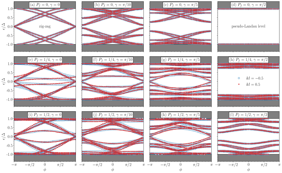
Figure 2: Andreev bound states (ABS) with different choice of $P_{f}$ and $\gamma$ and for two representative values of transverse momentum $kl=0.5$ (red) and $kl=-0.5$ (blue). The gray regions denote the continuum of states $\absolutevalue{\epsilon}>\Delta$. For (a) $P_{f}=0,\gamma=0$, we have the zig-zag modes in the network which has linearly dispersing ABS near zero energy. (a) is the ABS for zig-zag modes hosting zero energy states at $\phi=\pm\pi$. The zero-energy ABS persists if we increase $P_{f}$, while keeping $\gamma$ fixed at zero, see (a)$\to$(e)$\to$(i). As we increase $\gamma$ keeping $P_{f}$ constant, the ABS becomes gapped, and the bandwidth decreases, and at $P_{f}=0,\gamma=\pi/2$, it becomes perfectly flat for the pseudo-Landau level modes. We use $\theta=0.1^{\circ}$, $N=3$, $\Delta=1$ meV for these numerical plots.

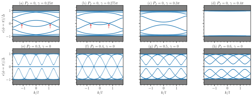
Figure 3: Andreev bound states (ABS) for $\phi=\pi$ over the first Brillouin zone, $kl\in[-2\pi/\sqrt{3},2\pi/\sqrt{3})$, for several values of $(P_{f},\gamma)$. (a)-(d) shows evolution of the ABS as we change $\gamma$ keeping $P_{f}=0$, the system evolves from a gapless-ABS spectrum to gapped-ABS state. The two Dirac-cones (indicated by red arrows) in the $k-\phi$ plane merges and gap out. (e)-(h) shows the evolution of ABS bands when we change $P_{f}\in[0.3,0.6]$ keeping $\gamma=0$ fixed. The ABS always have a momentum-independent zero energy mode at $\phi=\pi$ which disperses linearly in the $\phi$ direction (See Fig. 2). There is a gap-closing that happens at $P_{f}\approx 0.4$. For these numerical plots, we use $\theta=0.1^{\circ}$, $N=3$, and $\Delta=1$ meV.

III Andreev bound states and Josephson current

Modes with energies smaller than the superconducting gap ($\absolutevalue{\epsilon}\leq{\Delta}$) can not propagate through the superconductor. Consequently, they undergo multiple Andreev reflections at the superconducting interfaces, leading to the formation of bound states known as Andreev bound states (ABS). To find the ABS, we first note that $S_{\text{node}}$ and $S_{\text{bond}}$ matrices satisfy the equation $(\mathbb{I}-S_{\text{node}}S_{\text{bond}}(\epsilon,\phi))\bm{a}=0$. Then, for a non-trivial solution of $\bm{a}$, the following condition must hold:

$$\det(\mathbb{I}-S_{\text{node}}S_{\text{bond}}(\epsilon,\phi))=0.$$ (19)

The above determinantal equation is a transcendental equation that needs to be solved to find the energy of ABS ($\epsilon$) as a function of the superconducting phase difference $\phi$ and Bloch momentum $k$. The discrete ABS of the junction are denoted by ${\epsilon_{p}(\phi,k)}$, where $p$ represents the distinct ABS bands.

Each of the ABS at zero temperature ($T$) contributes to the Josephson current by an amount $J_{p}(\phi)=\frac{2e}{\hbar}\int\frac{\differential k}{2\pi}\derivative{\epsilon_{p}(\phi,k)}{\phi}$. Here, we adopt a more general framework [48, 46] to calculate the Josephson current at a finite temperature that takes into account the contribution coming from the quasiparticle continuum into the Josephson current as well. The expression of Josephson current reads,

$$J(\phi) =-k_{B}T\frac{2e}{\hbar}\int_{0}^{2\pi/\sqrt{3}l}\frac{\differential k}{2\pi}$$

$$\hskip 20.00003pt\times\derivative{\phi}\sum_{p=0}^{\infty}\ln\det[1-S_{\text{node}}(k)S_{\text{bond}}(i\Omega_{p},\phi)],$$ (20)

where the sum is over the fermionic Matsubara frequencies $\Omega_{p}=(2p+1)\pi k_{B}T$. Using Eq. (20), we compute the Josephson current numerically for different network parameters of MTBG. For $T\to 0$, the Matsubara summation becomes an integration, i.e., $k_{B}T\sum_{p}\to\int\frac{\differential\omega}{2\pi}$. Eq. (20) is valid under the assumption that the system reaches equilibrium without restrictions on the fermion parity; therefore, it holds for time scales that are much longer compared to the quasiparticle poisoning time [48]. This is the approximation we adopt in this work to compute the Josephson current. If this is not the case, corrections for parity conservation will be necessary [46].

Due to the large moiré length scale ($l$) for smaller $\theta$, the MTBG-Josephson junction naturally falls into the category of a long junction, where the junction length $L=Nl$ greatly exceeds the coherence length of the superconductor $\xi$ ($L\gg\xi$). The opposite limit ($L\ll\xi$) is dubbed as a short junction.

IV Numerical results

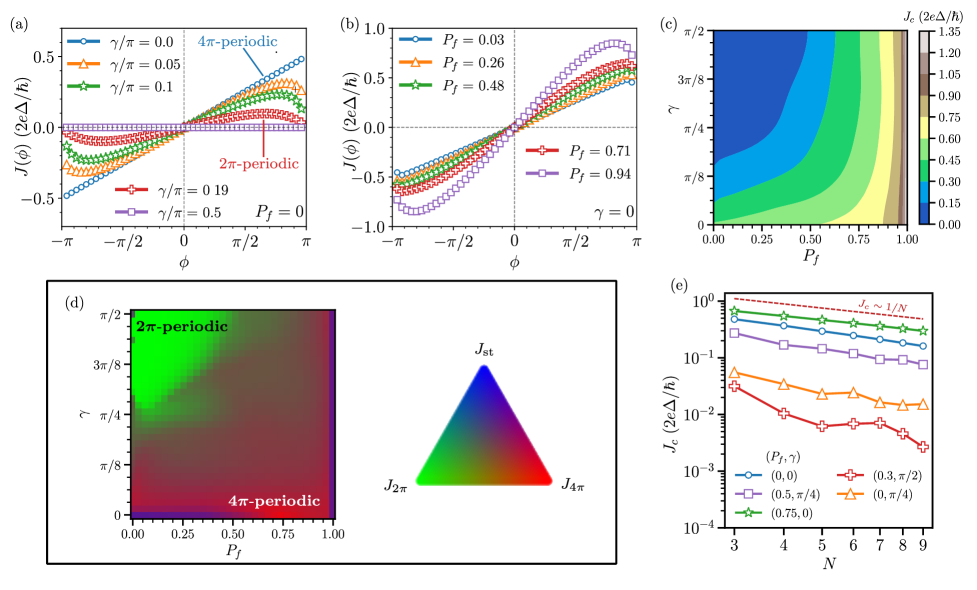
Figure 4: (a) Josephson current for $P_{f}=0$, and several values of $\gamma$. As we change $\gamma$ to go from the zig-zag modes to pseudo-Landau level modes, the Josephson current transforms from a $4\pi$ periodic sawtooth current profile to a $2\pi$ periodic sinusoidal current profile. For pseudo-Landau level modes ($P_{f}=0,\gamma=\pi/2$) the Josephson current becomes zero. (b) Josephson current for $\gamma=0$, and several values of $P_{f}$. By tuning $P_{f}$, the Josephson current changes from a sawtooth to a sinusoidal-sawtooth profile while maintaining the $4\pi$ periodicity. (c) Critical current for all values of $(P_{f},\gamma)$. The critical current is zero for the pseudo-Landau level modes ($P_{f}=0,\gamma=\pi/2$) and increases monotonically as we move away from this parameter by decreasing $\gamma$ and increasing $P_{f}$. (d) The Josephson current profile for all values of $(P_{f},\gamma)$. In the Josephson junction of MTBG, the current profile resembles one of the following: i) $2\pi$ periodic sinusoidal current ($J_{2\pi}$), ii) $4\pi$ periodic sinusoidal profile ($J_{4\pi}$) and iii) $4\pi$ periodic sawtooth profile ($J_{\mathrm{st}}$) represented by green, red and blue colors, respectively. The mixed character of $J_{\text{st}/2\pi/4\pi}$ is represented by the appropriate blending of red, green, and blue (see Eq. 24). (e) The critical current dependence on the length ($Nl$) of the Josephson junction for representative network parameters that show a $4\pi$ and $2\pi$ periodic Josephson current profile. For these numerical plots we use $\theta=0.1^{\circ}$, $\Delta=1$ meV and $T\ll\Delta=0.01\Delta$. For (a)–(d), we use $N=3$.

IV.1 Andreev bound-state (ABS) spectrum

In Fig. 2, ABS is illustrated for several values of the network parameters and two representative values of Bloch momentum $kl=\{-0.5,0.5\}$. The time reversal and particle-hole symmetry present in the system imposes that $\epsilon_{p}(\phi,k)=\epsilon_{p}(-\phi,-k)$ and $\epsilon_{p}(\phi,k)=-\epsilon_{-p}(\phi,-k)$, respectively. Moreover, the ABS spectrum is independent of Bloch momentum when the $P_{f}=0$ or $\gamma=\pi/2$. If we keep $\gamma=0$ and increase the value of $P_{f}$ (see Fig. 2 (a), (e), (i)), we find that the zero-energy crossing at $\phi=\pm\pi$ is robust under this change. On the contrary, with increasing $\gamma$, the zero energy crossing at $\phi=\pm\pi$ becomes fully gapped.

For the zig-zag (ZZ) modes, i.e., when $P_{f}=0$ and $\gamma=0$, the ABS near zero energy varies linearly as a function of the superconducting phase difference, i.e., $\epsilon\sim(\pi-\absolutevalue{\phi})$, featuring a zero energy crossing at $\phi=\pm\pi$. As the ABS merge into the quasiparticle continuum it becomes curved (see Fig. 2 (a)). Such ABS have been previously reported for a Josephson junction on the edge of a quantum spin Hall insulator [48]. With increasing $\gamma$ while keeping $P_{f}$ fixed at zero, the ABS are no longer linear in the phase difference. At the pseudo-Landau levels (pLL) parameter regime, i.e., when $P_{f}=0$ and $\gamma=\pi/2$, the MTBG hosts circulating modes and all the ABS above and below zero energy coalesce into two perfectly flat bands (see Fig. 2 (d)).

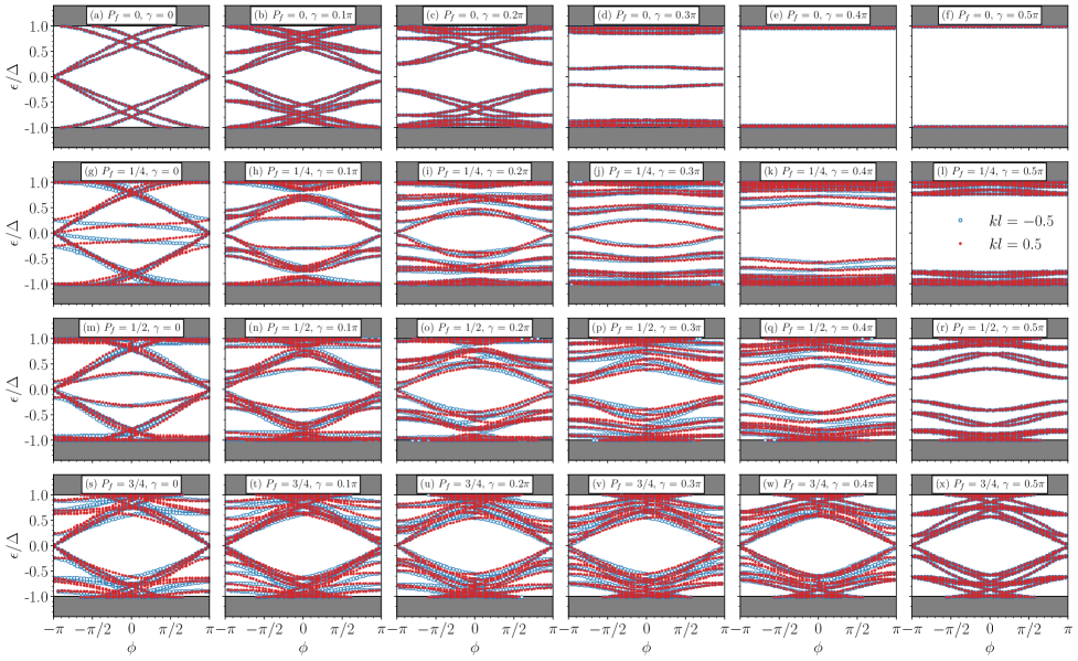
Figure 7: Extended Fig. 2 of main text. Andreev bound states (ABS) with different choice of $P_{f}$ and $\gamma$ and for two representative values of transverse momentum $kl=0.5$ (red) and $kl=-0.5$ (blue). The gray regions denote the continuum of states $\absolutevalue{\epsilon}>\Delta$. We use $\theta=0.1^{\circ}$, $N=3$, $\Delta=1$ meV for these numerical plots.

As we move away from $P_{f}=0$ and $\gamma=0$ line in the parameter space, many more ABS appear. For several network parameters (e.g., see Fig. 2 (f), (g), (j), (k) and also Fig. 7), we see that there coexist zero-enegy gapless and fully gapped ABS. As we discuss in following section, this coexistence results in a skewed Josephson current.

We also investigate the ABS with respect to Bloch momentum in Fig. 3. We particularly focus at $\phi=\pi$, where the presence of zero-energy ABS is plausible. For $P_{f}=0$ and for finite $\gamma$ (see Fig. 3 top panel), the ABS hosts zero energy states and forms two Dirac cones in the $k$–$\phi$ space. As we increase $\gamma$ while keeping $P_{f}$ fixed at zero, we see that the two Dirac cones merge at a certain value of $\gamma$ and gap out, and further increasing $\gamma$ makes the ABS flatter as we approach $\gamma=\pi/2$. This is how the ABS spectrum becomes gapped as one appraches the pLL limit. As we discuss below, this is also responsible for a crossover from a $4\pi$ to a $2\pi$ periodic Josephson current. Similarly, if we fix $\gamma$ to 0 and increase $P_{f}$ (see Fig. 3 bottom panel), the ABS always exhibits a zero energy state for all values of $P_{f}$. This is the zero energy ABS, which has a linear dependence on $\phi$ as mentioned previously (see Fig. 2 (a)). Upon increasing $P_{f}$, at a certain value of $P_{f}$, the gap between the zero-energy ABS and finite energy bands closes. However, this gap reappears as $P_{f}$ is increased further. During this ABS gap closing, the Josephson current changes from a sawtooth to a sinusoidal-sawtooth profile, as we discuss below.

IV.2 Josephson current

For the MTBG network, the Josephson responses have been summarized in the Fig. 4, where we observe that the form of Josephson current depends strongly on network parameters. We note that, the zero-energy level crossings in ABS induce a $4\pi$ periodicity of the Josephson current. On the other hand, gapped ABS always results in a $2\pi$ periodic Josephson current. As shown in Fig. 2, a combination of gapped and gapless ABS may also coexist for several network parameters. In such cases, Josephson current exhibits a mixed nature, comprising both $2\pi$ and $4\pi$ periodic components, resulting in a skewed current phase relationship.

As illustrated in Fig. 4 (a) in the zig-zag limit ($P_{f}=0,\gamma=0$), a sawtooth Josephson current is observed, i.e.,

$$J_{\text{st}}(\phi)\sim\frac{2e\Delta}{\hbar}\phi,\,\absolutevalue{\phi}<\pi,$$ (21)

with a discontinuity at $\phi=\pm\pi$. Such discontinuity in the Josephson current is a signature of $4\pi$ periodicity. This Josephson current profile resembles to that of a long normal metallic Josephson junction [49] and a long Josephson junction at the edge of a quantum spin Hall insulator [48]. This discontinuity arises from the presence of zero-energy Andreev bound states (ABS), as depicted in Fig. 2 (a) and Fig. 3 (a) and due to the assumption that the system equilibrates without any parity constraint. In this regime, perfect ballistic transmission is facilitated by the zig-zag modes, even when the forward scattering ($P_{f}$) is zero. Keeping $P_{f}$ fixed at zero, as we increase $\gamma$, the Josephson current profile changes from sawtooth ($J_{\text{st}}$) to a sinusoidal $2\pi$ periodic current, resembling a traditional Josephson current phase relation:

$$J_{2\pi}(\phi)\sim\frac{2e\Delta}{\hbar}\sin(\phi).$$ (22)

The $2\pi$ periodic Josephson current indicates that the ABS spectrum is fully gapped near zero-energy. The transition from $J_{\text{st}}$ to $J_{2\pi}$ occurs when two Dirac cones of ABS in the $k-\phi$ space merge and become fully gapped (see Fig. 3 top panel). Further increasing $\gamma$ leads to a decrease in the amplitude of the Josephson current, reaching zero finally at $\gamma=\pi/2$. This phenomenon can be attributed to the circulating modes for the pLL network parameters, which does not support transport through the bulk, as evidenced by the perfectly flat ABS (see Fig. 2 (d)).

On the other hand if we keep $\gamma$ fixed at 0, and increase $P_{f}$, the Josephson current profile transforms from a sawtooth to a sinusoidal $4\pi$-periodic Josephson current:

$$J_{4\pi}(\phi)\sim\frac{2e\Delta}{\hbar}\sin(\phi/2),\,\absolutevalue{\phi}<\pi.$$ (23)

There are zero-energy Andreev bound states present in the spectrum that facilitates this $J_{4\pi}$ periodic Josephson current. The transformation from $J_{\text{st}}$ to $J_{4\pi}$ happens at $P_{f}\approx 0.45$, that coincides with the value of $P_{f}$ where the gap between the zero-energy ABS and finite energy bands vanishes (see Fig. 3 bottom panel).

We study the dependence of critical current $J_{c}\,(=\max_{\phi}\absolutevalue{J(\phi)})$ in Fig. 4 (b), on the MTBG network parameters $P_{f}$ and $\gamma$. As mentioned previously, the critical current vanishes for pLL modes, i.e., $P_{f}=0$ and $\gamma=\pi/2$ and increases monotonically as we move away from that point by decreasing $\gamma$ and increasing $P_{f}$.

As one deviates from the $P_{f}=0$ and $\gamma=0$ lines in the parameter space, the Josephson current exhibits a combination of $J_{\text{st}/2\pi/4\pi}$ responses. We devise a method to determine which of the three responses or combinations thereof the Josephson current profile closely resembles. First, we normalize $J(\phi)$ so that it has the same amplitude as $J_{\text{st}/2\pi/4\pi}$. Then, the distances between the functions $J(\phi)$ and $J_{\text{st}/2\pi/4\pi}$ is calculated. This distance serves as a criterion to determine which current profile $J(\phi)$ resembles closely. The distance between two functions is formally defined as $||f-g||=\sqrt{\innerproduct{f-g}{f-g}}$, with the inner product defined as $\innerproduct{f}{g}=\int_{0}^{2\pi}\,\differential\phi f(\phi)g(\phi)/2\pi$. We construct a three tuple from the inverse distances as

$$\{u_{1},u_{2},u_{3}\}\propto\left\{\frac{1}{||J-J_{\text{s}t}||},\frac{1}{||J-J_{2\pi}||},\frac{1}{||J-J_{4\pi}||}\right\},$$ (24)

which is normalized such that $\sum_{i}u_{i}=1$. These three tuples $\{u_{1},u_{2},u_{3}\}$ represent the barycentric coordinates of an equilateral triangle. The coordinates: $\{1,0,0\}$, $\{0,1,0\}$, $\{0,0,1\}$ refer to the Josephson current profile of $\{J_{\text{st}},J_{2\pi},J_{4\pi}\}$, respectively. We assign the colors blue, green and red to these coordinates, respectively. For any other coordinates, we blend the colors (blue, green, red) in the ratio $\{u_{1},u_{2},u_{3}\}$. In this manner, we can discern which profile closely resembles $J(\phi)$.

The classification map of Josephson current is presented in Fig. 4 (d), across the entire parameter space of $(P_{f},\gamma)$. This map correctly captures the transition from $J_{\text{st}}$ to $J_{4\pi}$ at $P_{f}\approx 0.45$ and $\gamma=0$. Around the pLL parameters is a region where the Josephson current resembles $J_{2\pi}$. As $P_{f}$ reaches 1, irrespective of the values of $\gamma\in[0,\pi/2]$, the Josephson current profile becomes $J_{\text{st}}$ again. For most other regions of the parameter space, a mixed $J_{2\pi}$ and $J_{4\pi}$ character is observed. Fig. 4 (c), we also note From regions with the $J_{2\pi}$ Josephson current has a smaller critical current than that of $J_{\text{st}}$ and $J_{4\pi}$ regions.

In Fig. 4 (e), we show the dependence of the critical current as a function of the network length $Nl$, for various network parameters. For parameters resulting in a $4\pi$-Josephson current, we observe that the critical current decays as $\sim 1/(Nl)$. This behavior has been demonstrated for a long Josephson junction with normal metal barriers [49] and Josephson junction at the edge of a quantum spin Hall insulator [48]. For some representative values of parameters, this is shown in Fig. 4 (e). On the other hand, if the current is $2\pi$ periodic, the critical current decreases in a non-monotonic manner.

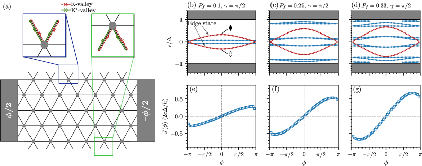
Figure 5: (a) The Josephson junction of a minimally twisted bilayer graphene with open top and bottom edges. At the edges, modes in K-valley are reflected back to K^′-valley and vice versa (see Eqs. 27, 28, 29 and 30). (b)–(d) Andreev bound states (ABS) and corresponding Josephson current (e)–(g) in the presence of open edges in the network. Then ABS, which arises in the presence of the edges, are annotated and shown in red. In the presence of pseudo-Landau level modes, the edges mediate the Josephson current, even if it is zero in the bulk. For the plots we use $\theta=0.1^{\circ}$, $(N_{x},N_{y})=(3,5)$, $\Delta=1$ meV and $T=0.01\Delta$.

V Effect of edges

So far, we imposed periodic boundary conditions in the transverse direction. In this section, we relax this condition and examine the impact of physical edges on ABS and Josephson current. In general, the geometric form of edges can be complicated because the relaxation at the boundaries of the MTBG can be different from that of the bulk. In order to understand the quantitative structure of the edges, extensive first-principle studies may be required, which, to the best of our knowledge, have not yet been documented in the literature. Following [50], we use a theoretical model of the edges and assume that the domain-wall modes of K-valley can be perfectly reflected back to K^′-valley up to a phase and vice versa at the edges (see Fig. 5 (a)). Such scatterings at the edges keep the network’s time reversal symmetry intact. This model additionally assumes that the truncation of the edges is located far away from the scattering nodes (i.e., AA regions) of the network. This is to ensure that the microscopic symmetries (Eq. (1) and (2)) of the scattering matrices near the edges are not destroyed. To this extent, we consider a finite network of size $(N_{x},N_{y})$, as shown in Fig. 5 (a).

The scattering matrix reads as follows:

$$\Xi^{(n,m)}=\mathcal{S}^{(n,m)}\oplus[\mathcal{S}^{(n,m)}]^{*}\oplus\mathcal{S}^{(n,m)}\oplus[\mathcal{S}^{(n,m)}]^{*},$$ (25)

$$S_{\text{node}}=\sigma_{0}\otimes\bigoplus_{n,m}\Xi^{(n,m)}.$$ (26)

The boundary condition for the domain-wall modes for the edges reads as follows: For the top edge, we have:

$$\bm{a}_{2\text{K}}^{(n,N_{y};\eta)} =\mathrm{diag}(e^{-i\psi_{1}},e^{i\psi_{1}},e^{-i\psi_{1}},e^{i\psi_{1}})\bm{b}_{2\text{K}^{\prime}}^{(n,N_{y};\eta)},$$ (27)

$$\bm{a}_{3\text{K}^{\prime}}^{(n,N_{y};\eta)} =\mathrm{diag}(e^{i\psi_{1}},e^{-i\psi_{1}},e^{i\psi_{1}},e^{-i\psi_{1}})\bm{b}_{3\text{K}}^{(n,N_{y};\eta)}.$$ (28)

Similarly, for the bottom edge, we have:

$$\bm{a}_{2\text{K}^{\prime}}^{(n,1;\eta)} =\mathrm{diag}(e^{-i\psi_{2}},e^{i\psi_{2}},e^{-i\psi_{2}},e^{i\psi_{2}})\bm{b}_{2\text{K}}^{(n,1;\eta)},$$ (29)

$$\bm{a}_{3\text{K}}^{(n,1;\eta)} =\mathrm{diag}(e^{i\psi_{2}},e^{-i\psi_{2}},e^{i\psi_{2}},e^{-i\psi_{2}})\bm{b}_{3\text{K}^{\prime}}^{(n,1;\eta)}.$$ (30)

Here, $i\in\{1,2,3\}$ in the subscript of the modes $\{i\xi\}$ refers to the three incoming and outgoing channels, $\xi\in\{\text{K},\text{K}^{\prime}\}$ is the valley index, $\eta\in\{1,2\}$ runs over two DW modes per valley, per spin. Here, $\bm{a}_{i\xi}^{(n,m;\eta)}$ and $\bm{b}_{i\xi}^{(n,m;\eta)}$ represent the amplitudes of the incoming and outgoing modes by four-dimensional vectors written in the basis of $\{e,h\}\otimes\{\uparrow,\downarrow\}$. $\psi_{1}$ and $\psi_{2}$ are the parameters associated with the reflection at the top and bottom edges, respectively. The ABS and Josephson current depends weakly on these parameters, and without loss of generality, we choose $\psi_{1}=\psi_{2}=0$ for our calculations.

In addition to Eq. (14) which describe the link connections in the MTBG and Eq. (17)–(18) which describe the connections between the MTBG network and superconducting leads, equations (27)–(28) are the newly introduced equations that are included in the $S_{\mathrm{bond}}$ matrix. Note that the superconducting leads connect the K and K^′ valleys through Andreev reflection, whereas the top and bottom edges of the network connect the two valleys via normal reflection.

We focus on the pseudo-Landau level regime because, in this parameter range, the bulk does not allow for any Josephson current. Instead, the Josephson current is mediated through the edges of the network created by the domain-wall modes.

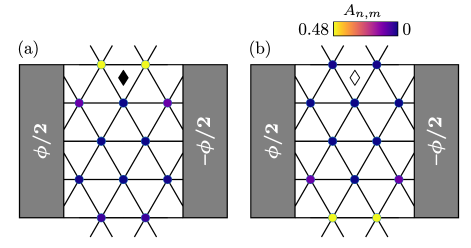
Figure 6: Amplitudes ($A_{n,m}$) of the incoming modes for the dispersive ABS shown in Fig. 5 (b). (a) shows the amplitudes for ABS marked by $\blacklozenge$ in Fig. 5 (b). The amplitude is localized on the top edge for this ABS. (b) shows the same for ABS marked by $\lozenge$. The amplitude is localized on the bottom edge. Here we use a network of size $(N_{x},N_{y})=(3,5)$.

We find the ABS by solving Eq. 19 with the modified $S_{\mathrm{node}}$ and $S_{\mathrm{bond}}$ matrices. The resulting ABS is shown in Fig. 5 (b)–(d). In Fig. 5 (b) for $P_{f}=0.1,\gamma=\pi/2$ we are in the vicinity of the pseudo-Landau level regime. We see that apart from two gapped flat ABS, two additional gapless (at $\phi=\pi$) dispersive ABS levels emerge because of the edges. In this regime, the level crossings of the flat and dispersive edges suggest that the bulk and edges of the network are decoupled. Note that the energy of the flat ABS are different from that of the bulk (see Fig. 2 (d)). This is a consequence of the finite size of the network in the transverse direction. As the value of $P_{f}$ is increased while keeping $\gamma=\pi/2$ fixed (refer to Fig. 5 (b), (c)), new ABS emerge with narrow bandwidth (similar to the bulk ABS spectrum, refer to Fig. 2 (h), (l)). However, the gapless dispersive ABS still persists. These ABS arises because of the edges is responsible for the large $4\pi$ periodic Josephson current, as we discuss below.

We compute the amplitude of incoming modes to demonstrate that the states correspond to gapless dispersive Andreev bound states localized at the network’s edges. The incoming mode ($\bm{a}$) for an ABS $\epsilon$ at superconducting phase difference $\phi$ belongs to the null-space of the operator $(\mathbb{I}-S_{\text{node}}S_{\text{bond}}(\epsilon,\phi))$, i.e.,

$$[\mathbb{I}-S_{\text{node}}S_{\text{bond}}(\epsilon,\phi)]\bm{a}=0$$ (31)

From the solution, the amplitude of the incoming mode ($A_{n,m}$) at $(n,m)$-th node is given by

$$A_{n,m}=\sum_{i=1}^{3}\sum_{\eta=1}^{2}\sum_{\xi\in\{\text{K},\text{K}^{\prime}\}}\left[\bm{a}_{i\xi}^{(n,m;\eta)}\right]^{\dagger}\bm{a}_{i\xi}^{(n,m;\eta)}.$$ (32)

$A_{n,m}$ is normalized, i.e., $\sum_{n,m}A_{n,m}=1$. The amplitudes of the nodes of the network are presented in Fig. 6. For $P_{f}=0.1$ and $\gamma=\pi/2$ (as illustrated in Fig. 5 (b)), we depict the amplitude for the positive and negative gapless dispersive ABS in Fig. 6 (a) and (b), respectively, with $\phi=0$. These amplitudes are localized at the top or the bottom edge of the network and decay in the bulk. This confirms that these ABS are indeed edge states.

As there is no additional summation over Bloch momentum, the Josephson current is now computed as:

$$J(\phi) =-k_{B}T\frac{2e}{\hbar}\derivative{\phi}\sum_{p=0}^{\infty}\ln\det[1-S_{\text{node}}S_{\text{bond}}(i\Omega_{p},\phi)].$$ (33)

In Fig. 5 (e), we see that near the pseudo-Landau level for $P_{f}=0.1,\gamma=\pi/2$ in the presence of the top and bottom edges, the current is finite, where it was vanishingly small for the bulk Josephson junction (please refer to Fig. 4 (a)). The Josephson current has a $4\pi$ periodic nature. As we increase the value of $P_{f}$ while keeping $\gamma=\pi/2$ in Fig. 5 (f), the critical current increases as a result of increased forward scattering while retaining the $4\pi$ periodic nature of the Josephson current. For larger values of $P_{f}$, the Josephson current also attains a $2\pi$ periodic component, thus making the Josephson current skewed as a function of $\phi$.

VI Discussion and summary

In this study, we have explored the Josephson junction comprising of a minimally twisted bilayer graphene (MTBG) sandwiched between two $s$-wave superconductors. Employing a Chalker-Coddington network model of MTBG, consistent with microscopic symmetries [34], we investigate the system’s transport phenomena across various network parameters. Depending on the network parameters of MTBG, the system exhibits distinct Andreev bound states (ABS) and Josephson currents. Specifically, for zig-zag modes, we observe the emergence of zero-energy Andreev bound states when the superconducting phase difference is $\pi$, leading to a $4\pi$ periodic Josephson current with a sawtooth profile. Conversely, in the case of pseudo-Landau level modes, the ABS manifests as a perfectly flat spectrum, resulting in the vanishing of the Josephson current when periodic boundary condition is assumed in the transverse direction. However, when edges are present in the network, the pseudo-Landau level modes can mediate a $4\pi$ periodic Josephson current through those edges even if the Josephson current in the bulk vanishes. This is similar to a skipping orbit of electrons transporting through the edge of a 2D electron gas in a magnetic field. Additionally, depending on the network parameters, the Josephson current may exhibit $2\pi$ periodicity, $4\pi$ periodicity, or a combined character of both.

The $4\pi$-periodic Josephson current has two distinct experimental signatures. Firstly, under constant DC bias ($V$), the oscillating Josephson current shows a dipolar Josephson emission at $f_{J}/2=eV/h$, typically in the GHz range, which can be measured using RF techniques [51]. Secondly, in the presence of an external microwave excitation at frequency $f$, Shapiro steps appear at discrete voltages given by $V_{n}=nhf/2e$, where $n$ is an integer step index. In the presence of a sizable $4\pi$-periodic Josephson current, only even steps (with missing odd steps) are expected [52, 53].

In our study, we have adopted a phenomenological approach, as the microscopic origins of $P_{f}$ and $\gamma$ remain unknown. In general, it may depend on the particulars of device fabrication, the value of the electric field, the twist angle, substrate potential, and other factors. From a physical perspective, beside the interlayer bias, the presence of a periodic potential, which can act as bias to the scattering nodes, can induce repulsion for the propagating domain-wall electrons, thereby effectively reducing the amplitude of forward scattering $P_{f}$. Tuning $\gamma$ is more challenging to achieve. One could apply a staggered magnetic field to append an additional phase to the domain wall modes, thus altering $\gamma$ while maintaining time reversal symmetry in the system. If such control can be achieved in practice, this would allow tuning of $P_{f}$ and $\gamma$ and in turn allow us to change the character of this Josephson junction and produce $2\pi$ and $4\pi$ periodic Josephson current on demand in situ.

Our study can also be adapted to recently discovered moiré systems, such as helical trilayer graphene [54]. Much like MTBG, this system also forms triangular domains due to lattice relaxation. In contrast to MTBG, helical trilayer graphene domains do not demonstrate AB/BA Bernal stacking; rather, each domain possesses a single-moiré periodic structure that is connected via $C_{2z}$ symmetry. Notably, if these domains can be gapped, electronic transport is primarily governed by domain-wall modes.

Appendix A Symmetry constraints on Scattering matrix

Following Ref. [55], we derive the action of symmetry operations on the scattering matrix. Below we only assume spin-less symmetries as minimally twisted bilayer graphene has spin-rotation symmetry intact.

A.1 Time reversal operation

In the spinless case, the time reversal operation is simply complex conjugation: $\mathcal{T}=\mathcal{K}$, where $\mathcal{K}$ denotes complex conjugation. Time reversal also interchanges the incoming and outgoing modes, with the action given by:

$$\mathcal{T}\bm{b}_{\text{out}}=\bm{a}^{*}_{\text{in}},\quad\mathcal{T}\bm{a}_{\text{in}}=\bm{b}^{*}_{\text{out}},$$ (34)

where $\bm{b}_{\text{out}}$ ($\bm{a}_{\text{in}}$) is the vector consisting of outgoing (incoming) modes.

Let $S_{+}$ and $S_{-}$ denote the scattering matrices for the time-forward and time-reversed processes, related by the $\mathcal{T}$ operator as:

$$S_{-}=\mathcal{T}S_{+}\mathcal{T}^{-1}.$$ (35)

For $S_{+}$, we have:

$$\bm{b}_{\text{out}}=S_{+}\bm{a}_{\text{in}}.$$ (36)

Acting the time reversal operation on this equation, we obtain:

$$\mathcal{T}\bm{b}_{\text{out}}=\mathcal{T}S_{+}\mathcal{T}^{-1}\mathcal{T}\bm{a}_{\text{in}},$$ (37)

$$\Rightarrow \bm{a}^{*}_{\text{in}}=S_{-}\bm{b}^{*}_{\text{out}},$$ (38)

$$\Rightarrow \bm{b}_{\text{out}}=S^{t}_{-}\bm{a}_{\text{in}}.$$ (39)

Here, $S^{t}_{-}$ denotes the transpose of $S_{-}$. To arrive at Eq. 39, we utilize Eqs. 35 and 34.

Thus, for time-reversal invariant systems, if we know the time-forward scattering matrix $S_{+}$, then $S_{-}=S^{t}_{+}$.

Moreover, if the scattering matrix is energy and momentum-dependent, after time reversal, the energy argument remains the same while the momentum changes sign. Hence, $S_{-}(E,k)=S^{t}_{+}(E,-k)$.

A.2 Charge conjugation operation

Charge conjugation interchanges particles and holes with a conjugation, i.e., $\mathcal{C}=\tau_{x}\mathcal{K}$, here, $\tau_{x}$ is the Pauli matrix acting on the particle-hole index. The action of charge conjugation operation on incoming and outgoing modes is given by:

$$\mathcal{C}\bm{b}_{\text{out}}=\tau_{x}\bm{b}^{*}_{\text{out}},\quad\mathcal{C}\bm{a}_{\text{in}}=\tau_{x}\bm{a}^{*}_{\text{in}}.$$ (40)

Let the scattering matrix of particle and hole sectors be denoted by $S_{p}$ and $S_{h}$, respectively. They are related by the charge conjugation operator:

$$S_{h}=\mathcal{C}S_{p}\mathcal{C}^{-1}.$$ (41)

For $S_{p}$ we have

$$\bm{b}_{\text{out}}=S_{p}\bm{a}_{\text{in}}.$$ (42)

Upon applying charge conjugation to both sides of Eq. 42, we obtain:

$$\mathcal{C}\bm{b}_{\text{out}}=\mathcal{C}S_{p}\mathcal{C}^{-1}\mathcal{C}\bm{a}_{\text{in}},$$ (43)

$$\Rightarrow \tau_{x}\bm{b}^{*}_{\text{out}}=S_{h}\tau_{x}\bm{a}^{*}_{\text{in}},$$ (44)

$$\Rightarrow \bm{b}_{\text{out}}=\tau_{x}S^{*}_{h}\tau_{x}\bm{a}_{\text{in}}.$$ (45)

Together Eqs. 42 and 45 imply $S_{h}=\tau_{x}S^{*}_{p}\tau_{x}$. For the case studied in the main text, the scattering matrix is for a normal metallic region diagonal in the particle-hole index. So, for that case, charge conjugation symmetry implies $S_{h}=S_{p}^{*}$.

In the case of an energy and momentum-dependent scattering matrix, charge conjugation flips the sign of both energy and momentum, yielding $S_{h}(E,k)=S_{p}^{*}(-E,-k)$.

Appendix B Details of the $S_{\text{bond}}$ matrix

This section details the construction of the $S_{\text{node}}$ matrix. Following each scattering event, the outgoing modes propagate freely for a duration of $\tau=l/v_{F}$, ($l$ is the moiré length scale and $v_{F}$ is the velocity of DW modes) before the subsequent scattering event. During this time, the DW modes acquire a dynamic phase $\xi\epsilon l/\hbar v_{F}$, where $\epsilon$ is the energy of the propagating modes. The valley index ($\xi$) in the dynamical phase accounts for the DW modes propagating in opposite directions in different valleys. After time $\tau$, we write down all the connections between the outgoing and incoming modes between the neighboring nodes. For K-valley, we have:

$$\bm{a}_{3\text{K}}^{(n,2;\eta)} =e^{i\epsilon l/v}\bm{b}_{3\text{K}}^{(n,1;\eta)},$$ (46)

$$\bm{a}_{2\text{K}}^{(n+1,1;\eta)} =e^{i\epsilon l/v}\bm{b}_{2\text{K}}^{(n,2;\eta)},$$ (47)

$$\bm{a}_{1\text{K}}^{(n,1;\eta)} =e^{i\epsilon l/v}\bm{b}_{1\text{K}}^{(n+1,1;\eta)},$$ (48)

$$\bm{a}_{1\text{K}}^{(n,2;\eta)} =e^{i\epsilon l/v}\bm{b}_{1\text{K}}^{(n+1,2;\eta)},$$ (49)

$$\bm{a}_{3\text{K}}^{(n+1,1;\eta)} =e^{i\epsilon l/v}\bm{b}_{3\text{K}}^{(n,2;\eta)},$$ (50)

$$\bm{a}_{2\text{K}}^{(n,2;\eta)} =e^{i\epsilon l/v}\bm{b}_{2\text{K}}^{(n,1;\eta)}.$$ (51)

Here, $i\in\{1,2,3\}$ in the subscript of the modes $\{i\xi\}$ refers to the three incoming and outgoing channels, $\eta\in\{1,2\}$ runs over two DW modes per valley, per spin. Here, $\bm{a}_{i\xi}^{(n,m;\eta)}$ and $\bm{b}_{i\xi}^{(n,m;\eta)}$ represent the amplitudes of the incoming and outgoing modes by four-dimensional vectors written in the basis of $\{e,h\}\otimes\{\uparrow,\downarrow\}$. For K^′-valley, the modes traverse in the opposite direction, resulting in a change in the sign of velocity ($v\to-v$). In other words, the incoming and outgoing modes interchange ($a\leftrightarrow b$) on the K^′-valley. The connections between outgoing and incoming modes between the neighboring nodes in the K^′-valley can be expressed as follows:

$$\bm{a}_{3\text{K}^{\prime}}^{(n,1;\eta)} =e^{i\epsilon l/v}\bm{b}_{3\text{K}^{\prime}}^{(n,2;\eta)},$$ (52)

$$\bm{a}_{2\text{K}^{\prime}}^{(n,2;\eta)} =e^{i\epsilon l/v}\bm{b}_{2\text{K}^{\prime}}^{(n+1,1;\eta)},$$ (53)

$$\bm{a}_{1\text{K}^{\prime}}^{(n+1,1;\eta)} =e^{i\epsilon l/v}\bm{b}_{1\text{K}^{\prime}}^{(n,1;\eta)},$$ (54)

$$\bm{a}_{1\text{K}^{\prime}}^{(n+1,2;\eta)} =e^{i\epsilon l/v}\bm{b}_{1\text{K}^{\prime}}^{(n,2;\eta)},$$ (55)

$$\bm{a}_{3\text{K}^{\prime}}^{(n,2;\eta)} =e^{i\epsilon l/v}\bm{b}_{3\text{K}^{\prime}}^{(n+1,1;\eta)},$$ (56)

$$\bm{a}_{2\text{K}^{\prime}}^{(n,1;\eta)} =e^{i\epsilon l/v}\bm{b}_{2\text{K}^{\prime}}^{(n,2;\eta)}.$$ (57)

At the superconducting electrodes, an electron of $K$ valley and $\uparrow$-spin is Andreev reflected as a hole of $K^{\prime}$ valley with $\downarrow$-spin and vice versa. As the links are made from one-dimensional DW modes, only retro Andreev reflection takes place, and specular Andreev reflection is suppressed [47]. The Andreev reflection is incorporated in the left and right lead via the following matrix:

$$M_{A}(\phi)=i\alpha\begin{pmatrix}0&0&0&-e^{i\phi}\\ 0&0&e^{i\phi}&0\\ 0&e^{-i\phi}&0&0\\ -e^{-i\phi}&0&0&0\end{pmatrix}.$$ (58)

$\alpha$ is defined as,

$$\alpha=\begin{cases}i\exp(-i\cos^{-1}\left({\epsilon}/{\Delta}\right))\quad\text{for }\epsilon\leq\Delta\\ i\exp(-\cosh^{-1}\left({\epsilon}/{\Delta}\right))\quad\text{for }\epsilon>\Delta,\end{cases}$$ (59)

where $\Delta$ and $\phi$ are the superconducting gap and phase, respectively. The Andreev reflection connects outgoing and incoming modes on the left superconducting junction as follows:

$$\bm{a}_{1\text{K}}^{(1,2;\eta)} =M_{A}(\phi/2)\bm{b}_{1\text{K}^{\prime}}^{(1,2;\eta)},$$ (60)

$$\bm{a}_{2\text{K}^{\prime}}^{(1,1;\eta)} =M_{A}(\phi/2)\bm{b}_{2\text{K}}^{(1,1;\eta)},$$ (61)

$$\bm{a}_{1\text{K}}^{(1,1;\eta)} =M_{A}(\phi/2)\bm{b}_{1\text{K}^{\prime}}^{(1,1;\eta)},$$ (62)

$$\bm{a}_{3\text{K}^{\prime}}^{(1,1;\eta)} =M_{A}(\phi/2)\bm{b}_{3\text{K}}^{(1,1;\eta)}.$$ (63)

Similarly, the connections at the right superconducting lead are given by:

$$\bm{a}_{1\text{K}^{\prime}}^{(N-1,2;\eta)} =M_{A}(-\phi/2)\bm{b}_{1\text{K}}^{(N-1,2;\eta)},$$ (64)

$$\bm{a}_{2\text{K}}^{(N,1;\eta)} =M_{A}(-\phi/2)\bm{b}_{2\text{K}^{\prime}}^{(N,1;\eta)},$$ (65)

$$\bm{a}_{1\text{K}^{\prime}}^{(N,1;\eta)} =M_{A}(-\phi/2)\bm{b}_{1\text{K}}^{(N,1;\eta)},$$ (66)

$$\bm{a}_{3\text{K}}^{(N,1;\eta)} =M_{A}(-\phi/2)\bm{b}_{3\text{K}^{\prime}}^{(N,1;\eta)}.$$ (67)

The equations (46)–(57) for the MTBG links and (60)–(67) for the superconducting leads and normal MTBG junction define the bond matrix $S_{\text{bond}}$ that acts on outgoing modes and returns incoming modes, i.e.,

$$\bm{a}=S_{\text{bond}}\bm{b}.$$

Appendix C Extended data for Andreev bound states

In this section, we present extended data of the Andreev bound state shown in the Fig. 2 for other values of network parameters.