Model- and Data-Based Control of Self-Balancing Robots: Practical Educational Approach with LabVIEW and Arduino

Abstract

A two-wheeled self-balancing robot (TWSBR) is non-linear and unstable system. This study compares the performance of model-based and data-based control strategies for TWSBRs, with an explicit practical educational approach. Model-based control (MBC) algorithms such as Lead-Lag and PID control require a proficient dynamic modeling and mathematical manipulation to drive the linearized equations of motions and develop the appropriate controller. On the other side, data-based control (DBC) methods, like fuzzy control, provide a simpler and quicker approach to designing effective controllers without needing in-depth understanding of the system model. In this paper, the advantages and disadvantages of both MBC and DBC using a TWSBR are illustrated. All controllers were implemented and tested on the OSOYOO self-balancing kit, including an Arduino microcontroller, MPU-6050 sensor, and DC motors. The control law and the user interface are constructed using the LabVIEW-LINX toolkit. A real-time hardware-in-loop experiment validates the results, highlighting controllers that can be implemented on a cost-effective platform.

1 Introduction

Contemporary control theory, or model-based control (MBC), originated with the parametric state-space model by Kalman Kalman (1960). MBC entails plant modeling or identification followed by controller design based on the assumed accuracy of the plant model, highlighting the crucial role of plant modeling and identification in MBC theory. Identification theory enables devising a plant model within a set that accurately represents the true system or closely approximates it, acknowledging that modeling, whether through first principles or data-driven identification, entails approximation and inevitable errors. Unmodeled dynamics are inherent in the modeling process, making closed-loop control systems designed using MBC approaches less secure due to these dynamics (Hou and Wang (2013)). With increasing complexity of modern processes, modeling using first principles or identification has become more challenging, rendering MBC less effective for modern-day plants. In such scenarios, data-based control (DBC) theory becomes critical, involving designing controllers directly using input-output data or data processing knowledge without relying on mathematical models (Hou and XU (2009)). In this study, a self-balancing robot was used as a test bed, akin to an inverted pendulum, maintaining balance by adjusting motor voltages to control wheel speed (Gonzalez et al. (2017)). Two-Wheeled Self-Balancing Robots (TWSBRs) are vital for testing control theories due to their unstable dynamics and nonlinearity, posing challenges as high-order, multivariable, nonlinear, tightly coupled, and inherently unstable systems as stated by Liang et al. (2018); Kim and Kwon (2022); Viswanathan et al. (2018). Balancing control for such a system is achieved through both linearized and nonlinear models (Kim and Kwon (2017); Shaban et al. (2014)). Recent studies have proposed various MBC methods for such systems, including well-established techniques such as Proportional Integral Derivative (PID) controllers as in T and K T (2021); Ren and Zhou (2021); Das et al. (2021); Shaban and Nada (2013) and DBC methods like Fuzzy Control (Susanto et al. (2020); Xu et al. (2013)) and Neural Network (NN) control as in Yang et al. (2014); Gandarilla et al. (2022); Homburger et al. (2023). These diverse approaches provide options for controlling systems like self-balancing robots, each with its advantages. This paper conducts a comprehensive analysis focusing on PID and lead-lag MBC methods and fuzzy DBC method, aiming to discern their efficacy in regulating self-balancing robots’ behavior. The paper is structured into six sections, starting with this overview. The subsequent section illustrates dynamic modelling and state-space representation, followed by examination of simulation framework and hardware configuration. The fourth section delves into design methodologies for PID controller, lead-lag compensator, and fuzzy logic controller, while the fifth section presents a comparative evaluation of these control strategies. Finally, the paper discusses research results and future directions.

2 System Modelling

In this section, the dynamic model of the TWSBR is derived using Lagrange equations, as referenced in Memarbashi and Chang (2011). The notation includes ’trans’ for translational and ’rot’ for rotational, with ’$C$’ representing the chassis and ’$W$’ for the wheel. A schematic showing the assignment of state variables is depicted in Fig. 1. Key parameters include: chassis mass $m,$ wheel mass $M$, wheel’s rotational inertia $J_{w}$, distance from chassis center of mass to wheel center $l$, wheel radius $R$, gravitational acceleration $g$, wheel-ground friction coefficient $\mu_{0}$, and and chassis-wheel axis friction coefficient $\mu_{1}$. $x_{p}$ is the position along $x$-axis, $\theta_{p}$ is the angle of the chassis inclination to the vertical axis, $z_{p}$ is the position in the $z$-axis, $\dot{x}_{p}$ and $\dot{z}_{p}$ are the linear velocities of the robot. These parameters are identified as $m=0.75\left[kg\right]$, $M=0.08\left[kg\right]$, $l=0.02$ $\left[m\right]$, $R=0.035\left[m\right]$, $\mu_{0}=0.1$, and $\mu_{1}=0$.

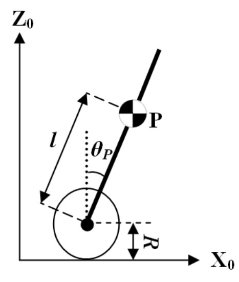
Figure 1: Kinematics of Robot Motion

2.1 Kinetic Energy

2.1.1 Chassis Kinetic Energy

The position and velocity of the robot chassis can be expressed as

$$\left.\begin{array}[]{c}x_{p}=x+l\text{ }s\theta_{p}\\ z_{p}=l\text{ }c\theta_{p}\end{array}\right\}\Leftrightarrow\left.\begin{array}[]{c}\dot{x}_{p}=v+l\omega_{p}\text{ }c\theta_{p}\\ \dot{z}_{p}=-l\omega_{p}\text{ }s\theta_{p}\end{array}\right\}$$

where $s\theta_{p}=\sin(\theta_{p})$, $c\theta_{p}=cos(\theta_{p})$, $v=\dot{x}$ is the velocity relative to the ground, and $\omega_{p}=\dot{\theta}_{p}$.The translating kinetic energy of the chassis can be expressed as

$$KE_{trans}^{C}=\frac{1}{2}m[\dot{x}_{p}^{2}+\dot{z}_{p}^{2}]=\frac{1}{2}m(v^{2}+l^{2}\omega_{p}^{2})+mvl\omega_{p}c\theta_{p}$$ (1)

The rotational $KE_{rot}^{C}$ of the robot can be expressed as $KE_{rot}^{C}=\frac{1}{2}J_{c}\omega_{p}^{2}$, where $J_{c}$ is the rotational Inertia of the chassis. Adding this term to Equ.1, yields total Kinetic Energy of the chassis ($KE_{total}^{C}$), as

$$KE_{total}^{C}=\frac{1}{2}m(v^{2}+l^{2}\omega_{p}^{2})+mvl\omega_{p}c\theta_{p}+\frac{1}{2}J_{c}\omega_{p}^{2}$$ (2)

2.1.2 Wheels Kinetic Energy

This is the energy due to the motion of the robot as a whole moving forward or backward. Each wheel of the robot also contributes to the total kinetic energy through its rotation. Thus, the kinetic energy of the two wheels ($KE_{total}^{W}$) of the robot can be expressed as

$$KE_{total}^{W}=KE_{trans}^{W}+KE_{rot}^{W}=Mv^{2}+J_{w}\frac{v^{2}}{R^{2}}$$ (3)

2.1.3 Total Kinetic Energy of the robot

The total kinetic energy of the system can be obtained from the combination of the wheels and chassis kinetic energies as

$$KE_{total} = KE_{total}^{C}+KE_{total}^{W}=\frac{1}{2}mv^{2}+\frac{1}{2}ml^{2}\omega_{p}^{2}$$ (4)

$$+mvl\omega_{p}c\theta_{p}+\frac{1}{2}J_{c}\omega_{p}^{2}+Mv^{2}+J_{w}\frac{v^{2}}{R^{2}}$$

2.2 Potential Energy and Dissipation Energy

The only form of potential energy in the system is the gravitational potential energy, which can be described as

$$PE_{total}=mglc\theta_{p}$$ (5)

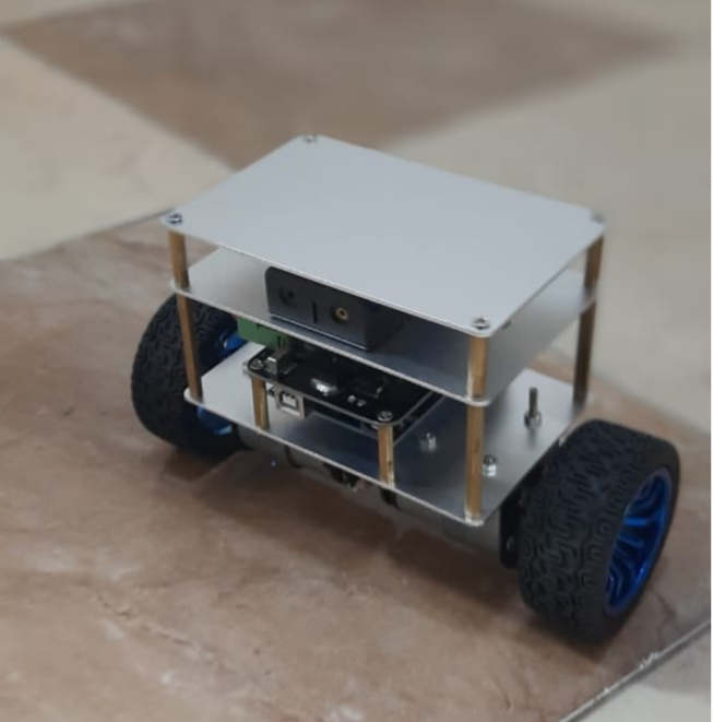
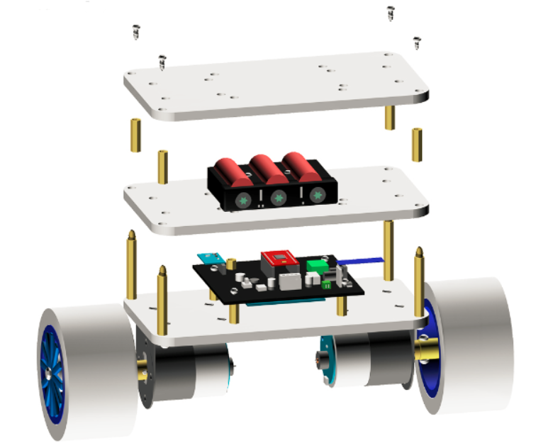
Figure 2: TWSBR live and CAD representation

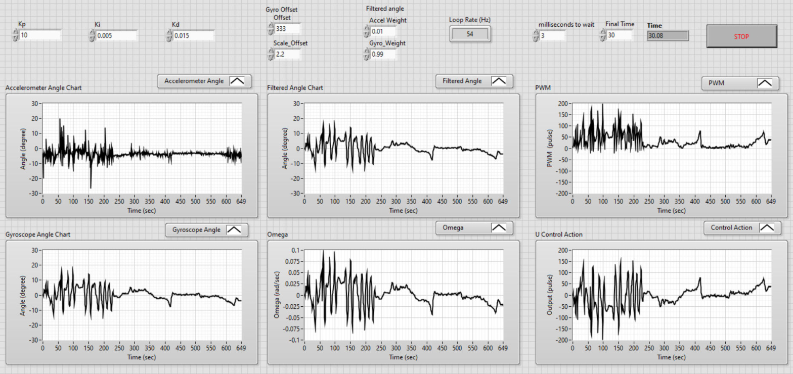
Figure 3: LabVIEW front panel of PID controlled system

On the other handm the only considerable dissipation that occurs within this system is the dissipation due to dry friction, which can be described as

$$F=\mu_{0}v^{2}+\mu_{1}\omega_{p}^{2}$$ (6)

where $\mu_{0}$ is the coefficient of friction between the wheels and the terrain, and $\mu_{1}$ is the coefficient of friction between the chassis and the wheels rotational axis. By using the Lagrange equation, the generalized external forces can be described as

$${\frac{{\partial}}{{\partial t}}\frac{\partial KE}{\partial\dot{q}_{i}}}-{\frac{{\partial KE}}{{\partial q_{i}}}}+{\frac{{\partial F}}{{\partial\dot{q}_{i}}}}+{\frac{{\partial PE}}{{\partial q_{i}}}}=Q_{i}$$ (7)

Here $q_{i}$ is a generalized state variable, and $Q_{i}$ is the external forces which is the torque exerted by the motors on the wheels. By substituting in the Lagrange equation (Equ 7), we get the two differential equations governing the dynamics of the system, Where $\tau_{L}+\tau_{R}$ are the left and right wheel torques respectively.

$$(m+2M+\frac{2J_{w}}{R^{2}})\ddot{x}+mlc\theta_{p}\ddot{\theta_{p}}+2\mu_{o}v=0$$ (8)

$$mlc\theta_{p}\ddot{x}+(ml^{2}+J_{c})\ddot{\theta_{p}}+2\mu_{1}\omega_{p}$$

$$+(mv\omega_{p}-mg)ls\theta_{p}=\tau_{L}+\tau_{R}$$ (9)

The Equations of motion, Equ 8 and Equ 9, represent a fully non-linear system. The linearlized form can be obtained by approximating $\sin\left(\theta_{p}\right)=\theta_{p}$ assuming $\theta_{p}$ is small and substituting $\cos\left(\theta_{p}\right)=1$, following the same premise. The linearized dynamic system equations can be formulated as

$$(m+2M+2\frac{J_{w}}{R^{2}})\ddot{x}+ml\ddot{\theta_{p}}+2\mu_{o}v = 0$$ (10)

$$ml\ddot{x}+(ml^{2}+J_{c})\ddot{\theta_{p}}+(mvlw_{p}-mgl)\theta_{p}+2\mu_{1}w_{p} = \tau_{L}+\tau_{R}$$

Defining the state vector as $\mathbf{x}^{T}=\begin{bmatrix}x&\theta_{p}&v&\omega_{p}\end{bmatrix}$, the state space representation is constructed from the dynamic equations (Equ 10 and LABEL:eq:lin3),

$$\mathbf{\dot{x}}=\mathbf{Ax}+\mathbf{B}u$$ (12)

where

$$\mathbf{A} = \begin{bmatrix}0&0&1&0\\ 0&0&0&1\\ 0&-\frac{(ml)^{2}g}{den}&-\frac{2\mu_{o}(ml^{2}+J_{c})}{den}&\frac{2ml\mu_{1}}{den}\\ 0&\frac{num}{den}&\frac{2\mu_{0}ml}{den}&-\frac{2\mu_{1}\ast num}{den}\end{bmatrix}$$

$$\mathbf{B}^{T} = \begin{bmatrix}0&0&-\frac{ml}{den}&\frac{num}{den}\end{bmatrix}$$

The system output can be described as $y=\mathbf{C}x$, where $\mathbf{C}$ as the output matrix. Particularly, $\mathbf{C}=$ $\begin{bmatrix}0&1&0&0\end{bmatrix}$ if $\theta_{p}$ is the system output. The terms $num=\left(m+2M+2\frac{J_{w}}{R^{2}}\right)$, and $den=\left(m+2M+2\frac{J_{w}}{R^{2}}\right)\left(ml^{2}+J_{c}\right)-(ml)^{2}$.

3 System and Control Implementation

Physical Hardware: In this study, the low cost OSOYOO TWSBR kit is utilized, which is a tool-set comprising two high-torque and high-speed gear motors. The TWSBR kit incorporates several components, including an Arduino UNO Board, Osyoo Balance Robot Shield, MPU6050 Module equipped with a $3-$axis Accelerometer and $3-$axis Gyroscope, a Bluetooth module, and a TB6612FNG driver Module. Fig. 2-(a) presents a live depiction of the TWSBR, while Fig. 2-(b) offers an exploded view from the designed CAD model, providing a detailed look at the internal components.
Control Design using LabVIEW: The CAD model was created in SOLIDWORKS, specifying the mass and inertia properties, with the simulated mass closely aligning with the actual mass of the robot ($802.45$ $grams$ in simulation compared to the measured $805$ $grams$). For the experimental setup, LabVIEW was utilized to develop the control system for the TWSBR. The front panel, see Fig. 3, is the interface for real-time PID control and data analysis. It provides inputs for PID gains $\left(K_{p},K_{i},K_{d}\right)$ constants for fine tuning based on the robot’s performance. The front panel visualizes the angles measured by the accelerometer and gyroscope, alongside a filtered angle that combines these readings for a stable angle measurement using a complementary filter whose weights are input by user. Additionally, it shows $\omega$, the angle’s rate of change, the control action (saturated between $[-255,255]$), and the unsigned PWM signals for the motors. The panel includes settings for experiment length, loop rate, and sensor calibration, offering adaptability for each test. The PID panel is tailored for its respective control, but the lead-lag and fuzzy panels only differ in specific gains and parameters, with a consistent overall design.

4 Controller Design

In the controller design process, the Arduino UNO’s utilized has high sampling rate ($16MHz)$, that can develop continuous-time transfer functions. With the system’s sampling rate at $200Hz$, considerably lower than $16MHz$, we were able to approximate the system to be in analog platform.

4.1 PID Controller Design

Initially, a PID controller was considered, but the presence of an open-loop pole on the right-hand side of the $s-$plane made Ziegler-Nichols tuning impractical, as shown in Fig. 6 which depicts the root locus of the TWSBR’s open-loop system. To overcome this and facilitate PID controller design, a graphical method using LabVIEW interfacing was adopted. The design is carried out by locating the zeros of the PD controller on the root locus to stabilize the system. The steady-state error required to further add the integral gain to optimize the performance of the system. The outcomes depicted in Fig. 6 represent the system’s response with applying specific gains determined through graphical analysis, resulting in a stable operating region.

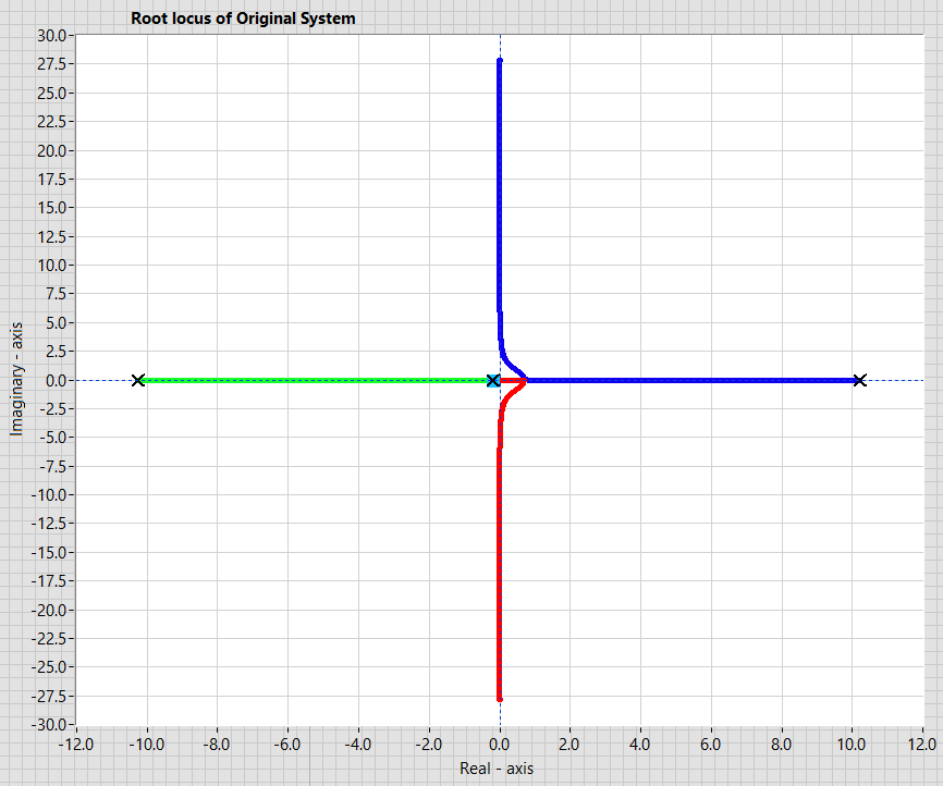
Figure 4: Root locus of the uncompensated system

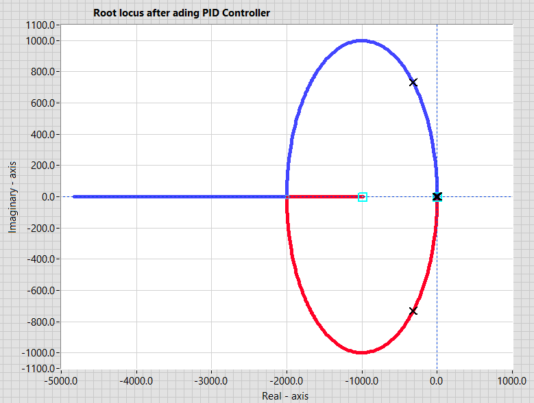
Figure 5: Root locus of PID controlled system: $K_{p}=10$, $K_{i}=0.005$, and $K_{d}=0.015$

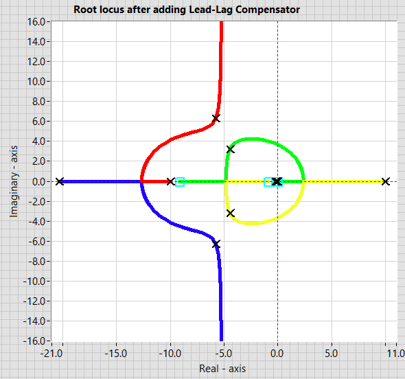
Figure 6: Root locus of Lead-lag compensated system: $K_{c}=3.25$ and $G_{c}(s)$ as in Equ.13

4.2 Design of Lead-lag Compensator

The lead-lag compensator enhances feedback control system performance by simultaneously addressing stability, transient response, and steady-state accuracy. Its primary function lies in introducing both phase lead and phase lag within the system’s frequency response. This dual-phase adjustment bolsters system stability by augmenting the phase margin, fortifying resilience against oscillations and instability. The phase lead improves transient response, facilitating accelerated response times, diminishing settling time, and mitigating oscillations for elevated dynamic performance. On the other hand, the phase lag refines the steady-state accuracy by attenuating higher-frequency components and adjusting the gain at lower frequencies, minimizing steady-state error, particularly in scenarios with disturbances. However, designing and deploying a lead-lag compensator requires careful consideration of inherent trade-offs in balancing stability, transient response, and steady-state accuracy. Achieving an optimal configuration involves analysis of system dynamics and performance requirements, often requiring sophisticated mathematical modeling and extensive tuning efforts. The system achieves stability through a lead-lag compensator, see Fig. 6, which displays the open-loop root locus of the compensated system. Design requirements included a settling time of $0.7[s]$ and a $6\%$ overshoot, achieved by positioning the poles and zeros on the root locus using the controller in Equ. 13. Specifically, the lead controller’s time constant is set to $0.1095[s]$ with an $\alpha=0.4494$, while the lag controller’s time constant is $1.123[s]$ with a $\beta=7.1439$  Additionally, the lead-lag controller gain $K_{c}$ is set to $3.25$.

$$G_{c}^{lead-lag}(s)=K_{c}\frac{0.13998s^{2}+1.40322s+1.1381}{s^{2}+20.4484s+2.53227}$$ (13)

4.3 Fuzzy Logic Controller (FLC)

The design process of a fuzzy logic controller involves three crucial stages: Fuzzification, where crisp inputs are transformed into fuzzy sets to handle linguistic variables and uncertainties in real-world systems; Fuzzy rule-based decision making, using predefined rules to guide the controller’s actions based on fuzzy inputs through complex decision spaces; and Defuzzification, where fuzzy control actions are converted into crisp values for practical implementation using methods such as centroid, mean of maximum (MOM), or weighted average.

By traversing through these stages, the FLC can process fuzzy inputs and generate precise control actions to steer complex systems towards desired outcomes. A notable implementation of FLC is the PID-like FLC, which combines proportional and derivative control elements Nada and Bayoumi (2024). This approach is advantageous in real-time applications on nonlinear mechatronic systems where traditional Model-Based Controllers may struggle. The PID-like FLC thus offers a versatile and efficient solution for controlling complex systems. In the practical implementation phase, we integrated the PID-like Fuzzy Logic Controller (FLC) as outlined by Nada and Bayoumi (2024). Transition to real-world applications was streamlined by easily adapting control parameters: PID Proportional Gain $K_{p}$ determines the error term’s proportional contribution to the control output; The Derivative Gain $K_{d}$ accounts for the contribution of the rate of change of the error term over time; Integral Gain $K_{i}$: compensates for accumulated past errors, aiding in the elimination of steady-state error;  and the FLC Proportional Gain $K_{u}$ influences the impact of fuzzy rules on the control action. In the implementation phase, we fine tuned the three gains explained before. We reached the balance using $K_{p}=150$, $K_{i}=1.5$, $K_{d}=1$, $K_{u}=1$, based on a trial and error approach which led to acceptable performance.

5 Results and Discussion

5.0.1 Experimental Validation

For a rigorous comparative analysis of the controllers’ performance, a $30[s]$ test duration was selected. This interval facilitated evaluating each controller’s impact on the tilting angle $\theta_{p}$, its rate of change ($\omega$), and motor control voltage, see Fig. 12, Fig. 12, and Fig. 12, respectively. To conduct this comparison and test the performance of each controller, we ensured consistency by using identical components and testing conditions throughout all experiments. We tested the robustness by introducing uncertainties to the system parameters where we added an additional mass to the platform and tested it with the same controller design and tuned gains, as shown in Fig. 12, Fig. 12, and Fig. 12.

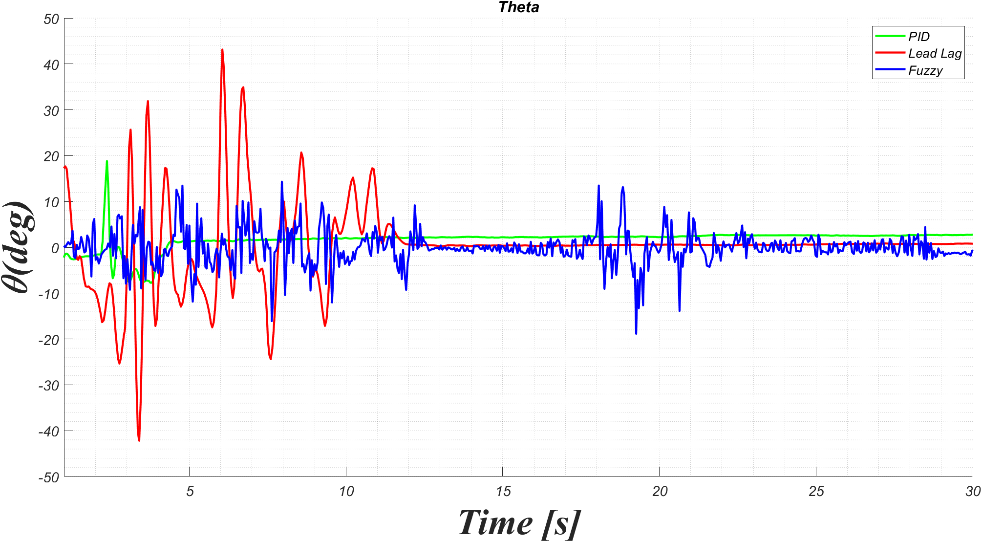
Figure 7: Effect of PID, lead lag, and FLC on $\theta_{p}$

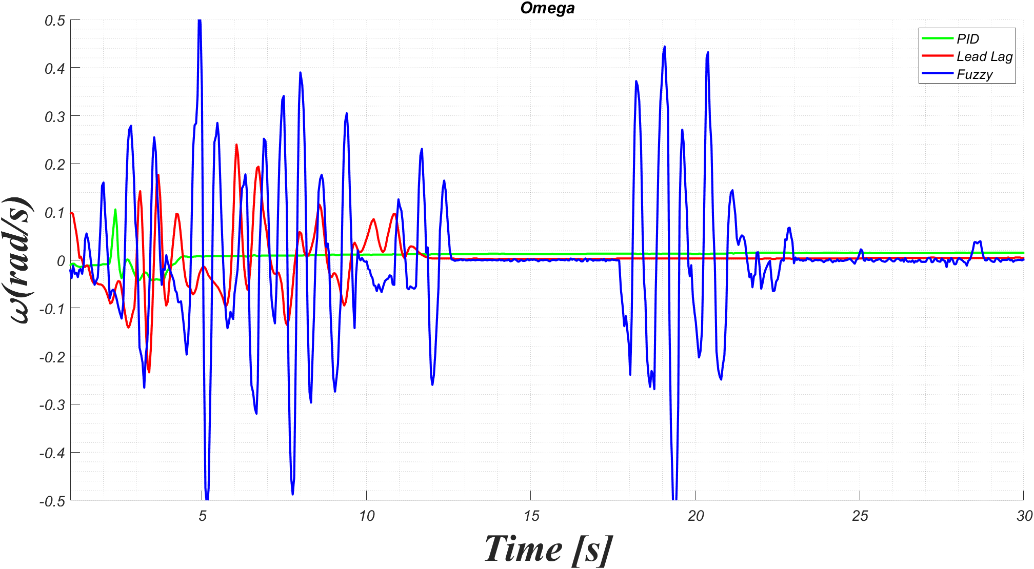
Figure 8: Effect of PID, lead lag, and FLC on $\omega$

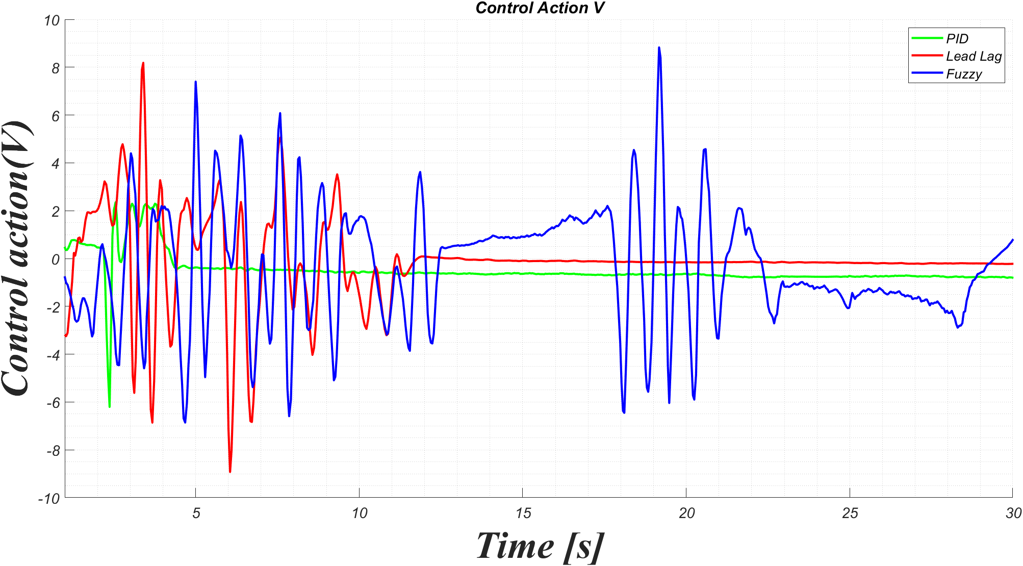
Figure 9: Effect of PID, lead lag, and FLC on control action

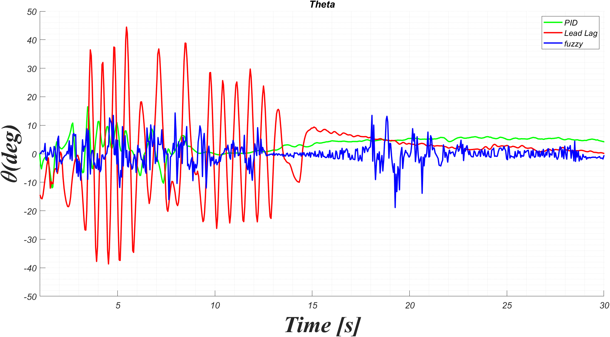
Figure 10: Effect of controllers on $\theta$ with mass uncertainty

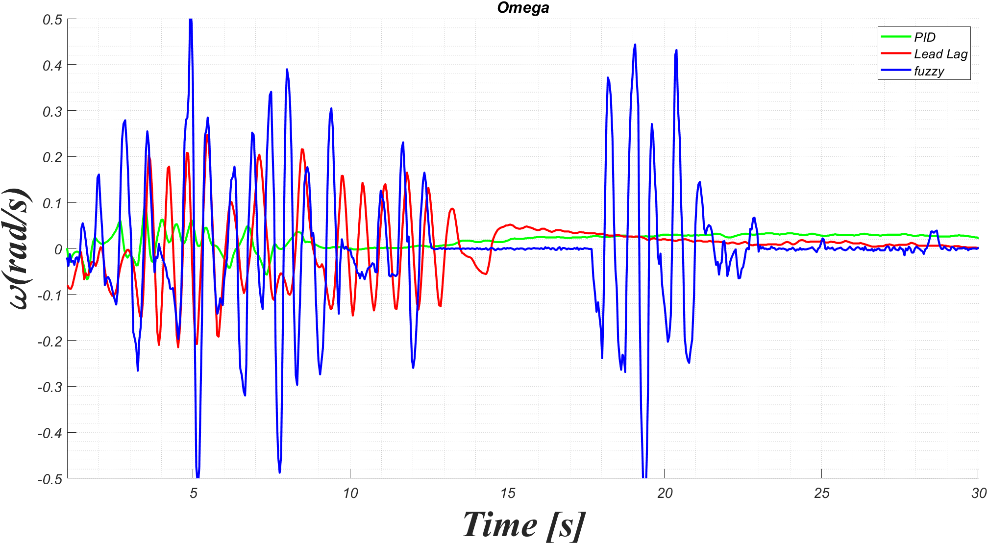
Figure 11: Effect of controllers on $\omega$ with mass uncertainty

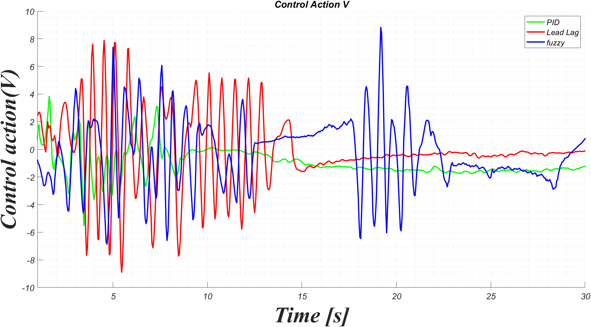
Figure 12: Effect of controllers on control action with mass uncertainty

5.0.2 Evaluation Metrics

1. Steady-State Accuracy: MBC classical approaches (PID - lead lag) are the most efficient for regulating the tilt angle, see Fig. 12 and their exclusive behaviour on the change of $\omega$ as shown in Fig. 12 with PID being slightly better.

2. Settling Time: Regarding settling time, MBC methods outperform, with PID and lead-lag controllers reaching settling times of $5$ and $12[s]$, respectively. In contrast, the DBC strategy, specifically the FLC, attains a settling time of $27[s]$, as depicted in Fig. 12.

3. Ease of Design: FLC does not require a predefined mathematical model, simplifying its design compared to MBC approaches. However, the aggressive control action of FLC, as shown in Fig. 12, may not be cost-efficient. Nonetheless, FLC is ideal for quick model-free implementations.

4. Tuning Complexity:Regarding the ease of design, PID and lead-lag controllers allow for straightforward implementation once detailed design is complete. Conversely, although Fuzzy Logic Controllers (FLC) have a relatively simple design process, their tuning is complex and time-consuming.

5. Robustness: When adding an additional mass to induce uncertainties in the model to test robustness, All of PID, lead lag and FLC controllers could maintain the platform stable in Fig. 12, Fig. 12, and Fig. 12. The PID controller had the best performance having the lowest overshoot and settling time as shown in Fig. 12, with less aggressive control actions as in Fig. 12 which makes the angle rate of change low, see Fig. 12. We can see that the FLC was not able to reach the steady state within the 30 seconds trial while also having the greatest overshoot.

6 Conclusion

This study presents a comparative analysis between Model-Based Control (MBC) and Data-Based Control (DBC) strategies, specifically the PID, lead-lag, and fuzzy logic for stabilizing a Two-Wheeled Self-Balancing Robot. A comprehensive control framework is established, including the state-space model, LabVIEW interface, and real-time prototyping of the robot. The analysis highlights the the distinct performance characteristics of each method. MBC methods, particularly PID and lead-lag controls, show better accuracy, minimum error, faster response, and high robustness, making them suitable for precise control requirements. Despite the ease of design with fuzzy logic controllers (FLC), they tend to have more fluctuated control actions and need a relatively complicated tuning procedure. It is suggested that FLC’s performance could be optimized by specific tuning of its membership functions and rules. The introduced framework throughout the paper enables young engineers to realize the control system design, and improve their skills toward system optimization and real-time implementation.

References

- Das et al. [2021] Das, A., Rahman, M., Adib, A., and Anam, M. (2021). Self-balancing robot with pid controller.
- Gandarilla et al. [2022] Gandarilla, I., Montoya-Cháirez, J., Santibáñez, V., Aguilar-Avelar, C., and Moreno-Valenzuela, J. (2022). Trajectory tracking control of a self-balancing robot via adaptive neural networks. Engineering Science and Technology, an International Journal, 35, 101259.
- Gonzalez et al. [2017] Gonzalez, C., Alvarado, I., and La Peña, D.M. (2017). Low cost two-wheels self-balancing robot for control education. IFAC-PapersOnLine, 50(1), 9174–9179.
- Homburger et al. [2023] Homburger, H., Wirtensohn, S., Diehl, M., and Reuter, J. (2023). Comparison of data-driven modeling and identification approaches for a self-balancing vehicle. IFAC-PapersOnLine, 56(2), 6839–6844. https://doi.org/10.1016/j.ifacol.2023.10.611. 22nd IFAC World Congress.
- Hou and Wang [2013] Hou, Z. and Wang, Z. (2013). From model-based control to data-driven control: Survey, classification and perspective. Information Sciences, 235, 3–35. 10.1016/j.ins.2012.07.014.
- Hou and XU [2009] Hou, Z. and XU, J.X. (2009). On data-driven control theory: the state of the art and perspective. Acta Automatica Sinica, 35, 650–667. 10.3724/SP.J.1004.2009.00650.
- Kalman [1960] Kalman, R.E. (1960). A New Approach to Linear Filtering and Prediction Problems. Journal of Basic Engineering, 82(1), 35–45. 10.1115/1.3662552. URL https://doi.org/10.1115/1.3662552.
- Kim and Kwon [2017] Kim, S. and Kwon, S. (2017). Nonlinear optimal control design for underactuated two-wheeled inverted pendulum mobile platform. IEEE/ASME Transactions on Mechatronics, PP, 1–1. 10.1109/TMECH.2017.2767085.
- Kim and Kwon [2022] Kim, Y. and Kwon, S. (2022). Robust stabilization of underactuated two-wheeled balancing vehicles on uncertain terrains with nonlinear-model-based disturbance compensation. Actuators, 11(11). 10.3390/act11110339.
- Liang et al. [2018] Liang, D., Sun, N., Wu, Y., and Fang, Y. (2018). Differential flatness-based robust control of self-balanced robots. IFAC-PapersOnLine, 51(31), 949–954.
- Memarbashi and Chang [2011] Memarbashi, H. and Chang, J.Y. (2011). Design and parametric control of co-axes driven two-wheeled balancing robot. Microsystem Technologies, 17, 1215–1224. 10.1007/s00542-010-1213-7.
- Nada and Bayoumi [2024] Nada, A. and Bayoumi, M. (2024). Development of embedded fuzzy control using reconfigurable fpga technology. Automatika, 65, 609–626. 10.1080/00051144.2024.2313904.
- Ren and Zhou [2021] Ren, H. and Zhou, C. (2021). Control system of two-wheel self-balancing vehicle. Journal of Shanghai Jiaotong University (Science), 26, 713–721.
- Shaban and Nada [2013] Shaban, E.M. and Nada, A.A. (2013). Proportional Integral Derivative versus Proportional Integral plus Control Applied to Mobile Robotic System. Journal of American Science, 9(12).
- Shaban et al. [2014] Shaban, E., Nada, A., and Taylor, C. (2014). Exact linearization by feedback of state dependent parameter models applied to a mechatronics demonstrator. In 2014 UKACC International Conference on Control, CONTROL 2014 - Proceedings. 10.1109/CONTROL.2014.6915209.
- Susanto et al. [2020] Susanto, E., Surya Wibowo, A., and Ghiffary Rachman, E. (2020). Fuzzy swing up control and optimal state feedback stabilization for self-erecting inverted pendulum. IEEE Access, 8, 6496–6504. 10.1109/ACCESS.2019.2963399.
- T and K T [2021] T, N. and K T, P. (2021). Pid controller based two wheeled self balancing robot. In 2021 5th International Conference on Trends in Electronics and Informatics (ICOEI), 1–4. 10.1109/ICOEI51242.2021.9453091.
- Viswanathan et al. [2018] Viswanathan, S.P., Sanyal, A.K., and Samiei, E. (2018). Integrated guidance and feedback control of underactuated robotics system in se (3). Journal of Intelligent & Robotic Systems, 89, 251–263.
- Xu et al. [2013] Xu, J.X., Guo, Z.Q., and Lee, T. (2013). Design and implementation of a takagi–sugeno-type fuzzy logic controller on a two-wheeled mobile robot. Industrial Electronics, IEEE Transactions on, 60, 5717–5728. 10.1109/TIE.2012.2230600.
- Yang et al. [2014] Yang, C., Li, Z., Cui, R., and Xu, B. (2014). Neural network-based motion control of an underactuated wheeled inverted pendulum model. IEEE Transactions on Neural Networks and Learning Systems, 25(11), 2004–2016. 10.1109/TNNLS.2014.2302475.