CCDM: Continuous Conditional Diffusion Models for Image Generation

Abstract

Continuous Conditional Generative Modeling (CCGM) aims to estimate the distribution of high-dimensional data, typically images, conditioned on scalar continuous variables known as regression labels. While Continuous conditional Generative Adversarial Networks (CcGANs) were initially designed for this task, their adversarial training mechanism remains vulnerable to extremely sparse or imbalanced data, resulting in suboptimal outcomes. To enhance the quality of generated images, a promising alternative is to replace CcGANs with Conditional Diffusion Models (CDMs), renowned for their stable training process and ability to produce more realistic images. However, existing CDMs encounter challenges when applied to CCGM tasks due to several limitations such as inadequate U-Net architectures and deficient model fitting mechanisms for handling regression labels. In this paper, we introduce Continuous Conditional Diffusion Models (CCDMs), the first CDM designed specifically for the CCGM task. CCDMs address the limitations of existing CDMs by introducing specially designed conditional diffusion processes, a modified denoising U-Net with a custom-made conditioning mechanism, a novel hard vicinal loss for model fitting, and an efficient conditional sampling procedure. With comprehensive experiments on four datasets with varying resolutions ranging from $64\times 64$ to $192\times 192$, we demonstrate the superiority of the proposed CCDM over state-of-the-art CCGM models, establishing new benchmarks in CCGM. Extensive ablation studies validate the model design and implementation configuration of the proposed CCDM. Our code is publicly available at https://github.com/UBCDingXin/CCDM.

I Introduction

Continuous Conditional Generative Modeling (CCGM), as depicted in Fig. 1, aims to estimate the probability distribution of images conditioned on scalar continuous variables. These variables, often termed regression labels, can encompass angles, ages, temperatures, counting numbers, and more. The scarcity of training samples for certain regression labels and the lack of a suitable label input mechanism render CCGM a highly challenging task.

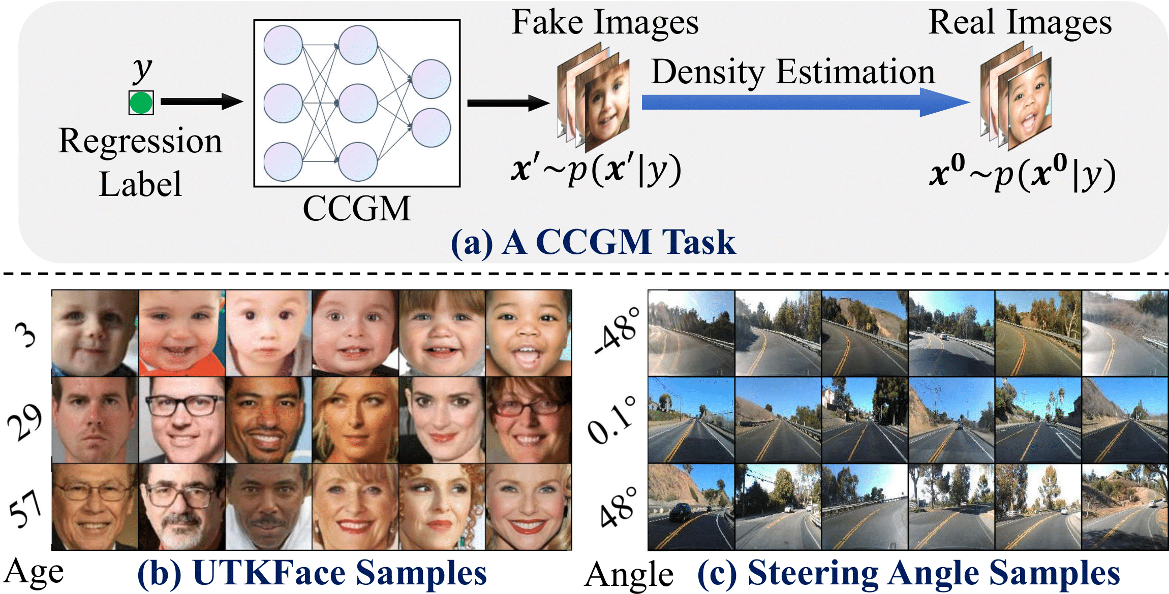
Figure 1: Illustration of the CCGM task with sample images from the UTKFace and Steering Angle datasets.

As a recent advancement, Ding et al. [ding2023ccgan] introduced the first feasible model to the CCGM task, termed Continuous conditional Generative Adversarial Networks (CcGANs). CcGANs address existing challenges in CCGM by devising novel vicinal discriminator losses and label input mechanisms. Consequently, CcGANs have been extensively applied across various domains requiring precise control over generative modeling of high-dimensional data. These applications comprise engineering inverse design [heyrani2021pcdgan, fang2023diverse, zhao2024ccdpm], data augmentation for hyperspectral imaging [zhu2023data], remote sensing image processing [giry2022sar], model compression [ding2023distilling], controllable point cloud generation [triess2022point], carbon sequestration [stepien2023continuous], data-driven solutions for poroelasticity [kadeethum2022continuous], and more. However, as reported in [ding2024turning], the training process of CcGANs remains susceptible to extremely sparse or imbalanced training data due to the unstable adversarial mechanism, resulting in suboptimal outcomes.

Diffusion models, emerging as another class of generative models, have garnered significant attention recently. Compared to Generative Adversarial Networks (GANs) [goodfellow2014generative, mirza2014conditional, kang2021rebooting, hou2022conditional, 10041783, 10296870], diffusion models offer a substantially more stable training process and produce more realistic samples [dhariwal2021diffusion, ho2021classifier, rombach2022high, peebles2023scalable]. Given this, it seems logical to abandon the unstable adversarial mechanism in favor of diffusion models to stabilize model training and produce more realistic samples in the CCGM task. Nonetheless, as mentioned by Ding et al. [ding2024turning], Conditional Diffusion Models (CDMs), including classifier guidance models [dhariwal2021diffusion] and classifier-free guidance models [ho2021classifier, rombach2022high, peebles2023scalable], encounter challenges when dealing with regression labels. These challenges stem from several factors: (1) Their U-Net architectures do not adequately support scalar continuous conditions; (2) Their model fitting does not account for scenarios with very few or zero training data points for certain regression labels; (3) Some configurations of CDMs, originally designed for discrete conditions or multi-dimensional continuous conditions, are inapplicable to regression labels. Hence, current CDMs are inapplicable to the CCGM task.

Motivated by the aforementioned issues, we propose in this paper the Continuous Conditional Diffusion Models (CCDMs), designed to overcome the limitations of existing CDMs and enhance their suitability for the CCGM task. We address several obstacles encountered when integrating CDMs into CCGM. Our contributions and the paper’s structure can be summarized as follows:

• We introduce conditional forward and reverse diffusion processes that take into account the regression labels in Section III-A.

• We propose in Section III-B a modified denoising U-Net architecture featuring a conditioning mechanism custom-made for regression labels $y$.

• To mitigate the issue of data scarcity, we propose a novel hard vicinal loss for model fitting in Section III-C.

• Leveraging the trained U-Net and the DDIM sampler [song2021denoising], we devise an efficient and effective conditional sampling algorithm in Section III-D.

• We present comprehensive experiments showcasing the superior performance of CCDMs in Section IV, accompanied by meticulously crafted ablation studies aimed at assessing the impact of various configurations for the proposed method in Section LABEL:sec:ablation.

It is important to note that our proposed CCDM differs significantly from a concurrent work named CcDPM [zhao2024ccdpm]:

• CcDPM, as a conditional diffusion model, is tailored for non-image data with multi-dimensional continuous labels, which means it lacks a suitable conditioning mechanism for regression labels. In contrast, the proposed CCDMs are specifically designed for generative modeling of image data conditioned on scalar continuous labels, providing an effective conditioning mechanism for regression labels. Therefore, the proposed CCDM represents the first CDM designed specifically for the CCGM task.

• The training loss for CcDPM relies on the noise prediction error, whereas for CCDMs, the loss is derived from image denoising. Our ablation study shows that the noise prediction-based loss yields inferior performance in the CCGM task.

• CcDPM utilizes the soft vicinity approach to define a weighted training loss for diffusion models. However, we advocate using the hard vicinity instead, as it demonstrates superior label consistency compared to the soft approach in our ablation study.

These distinctions highlight the unique focus and effectiveness of CCDMs in the context of generative modeling with scalar continuous labels for image data.

II Related Work

II-A Continuous Conditional GANs

CcGANs, introduced by Ding et al. [ding2021ccgan, ding2023ccgan], represent the pioneering approach to the CCGM task. As shown in Fig. 1, mathematically, CcGANs are devised to estimate the probability density function $p(\bm{x}^{0}|y)$, characterizing the underlying conditional data distribution, where $y$ represents regression labels. In addressing concerns regarding the potential data insufficiency at $y$, Ding et al. [ding2021ccgan, ding2023ccgan] posited an assumption wherein minor perturbations to $y$ result in negligible alterations to $p(\bm{x}^{0}|y)$. Building upon this assumption, they formulated the Hard and Soft Vicinal Discriminator Losses (HVDL and SVDL) alongside a novel generator loss, aimed at enhancing the stability of GAN training. Furthermore, to overcome the challenge of encoding regression labels, Ding et al. [ding2021ccgan, ding2023ccgan] proposed both a Naïve Label Input (NLI) mechanism and an Improved Label Input (ILI) mechanism to effectively integrate $y$ into CCGM models. The ILI approach employs a label embedding network $\phi$ comprising a 5-layer perceptron to map the scalar $y$ to a $128\times 1$ vector $\bm{h}_{y}$, i.e.,$\bm{h}_{y}=\phi(y)$. This vector, $\bm{h}_{y}$, is then fed into the generator and discriminator networks of CcGANs to control the generative modeling process. The efficacy of CcGANs has been demonstrated by Ding et al. [ding2021ccgan, ding2023ccgan] and other researchers [heyrani2021pcdgan, wang2021image, giry2022sar, zhu2023data] across diverse datasets, showcasing their robustness and versatility in various applications. However, as pointed out in [ding2024turning], the adversarial training mechanism is vulnerable to data insufficiency, and CcGANs may still generate subpar fake images. Therefore, in this paper, we propose to transition away from the fragile adversarial mechanism and instead adopt conditional diffusion processes for the CCGM task, while retaining the vicinal training and label input mechanisms from the previous method.

II-B Diffusion Models

As a substitute for GANs, diffusion models offer another feasible approach for generative modeling and have been applied across numerous computer vision tasks [croitoru2023diffusion, yang2023diffusion, 10480591, 10261222, 10321681].

A notable example is Denoising Diffusion Probabilistic Models (DDPMs) [ho2020denoising]. DDPMs encompass a forward diffusion process and a reverse diffusion process, both of which are modeled using Markov chains. The forward diffusion process gradually transforms a real image $\bm{x}^{0}\sim p(\bm{x}^{0})$ into pure Gaussian noise $\bm{x}^{T}\sim\mathcal{N}(\bm{0},\bm{I})$ through $T$ steps of transitions $q(\bm{x}^{t}|\bm{x}^{t-1})$, where $T$ is sufficiently large. Then, a learnable reverse process gradually converts $\bm{x}^{T}$ back to $\bm{x}^{0}$ with $T$ steps of transitions $p_{\bm{\theta}}(\bm{x}^{t-1}|\bm{x}^{t})$, where $\bm{\theta}$ represents learnable parameters. The training loss for DDPMs takes the form of a noise prediction error:

$$L_{simple}(\bm{\theta})=\mathbb{E}_{\bm{\epsilon},\bm{x}^{t}}\|\hat{\bm{\epsilon}}_{\bm{\theta}}(\bm{x}^{t},t)-\bm{\epsilon}\|^{2}_{2}$$ (1)

where $\hat{\bm{\epsilon}}_{\bm{\theta}}(\bm{x}^{t},t)$ is modeled by a U-Net [ronneberger2015u]. This U-Net is trained to predict the ground truth sampled Gaussian $\bm{\epsilon}\sim\mathcal{N}(\bm{0},\bm{I})$. Despite its ability to generate high-quality data, DDPMs often grapple with long sampling times. To address this, Song et al. introduced Denoising Diffusion Implicit Models (DDIMs) [song2021denoising]. DDIMs offer a deterministic but shorter reverse process, enabling the generation of high-quality samples with significantly fewer time steps than DDPMs.

Unlike DDPMs, which aim to estimate the marginal data distribution $p(\bm{x}^{0})$, Ho et al. [ho2021classifier] introduced the Classifier-Free Guidance (CFG) model to estimate the conditional distribution $p(\bm{x}^{0}|y)$. As a CDM, CFG integrates class labels as conditions and employs the following equation for sampling [luo2022understanding]:

$$\triangledown\log p(\bm{x}^{t}|y)=(1-\gamma)\triangledown\log p(\bm{x}^{t})+\gamma\triangledown\log p(\bm{x}^{t}|y)$$ (2)

where $\triangledown\log p(\bm{x}^{t}|y)$ is an abbreviation of the score function $\triangledown_{\bm{x}^{t}}\log p(\bm{x}^{t}|y)$, $y$ represents class labels, and $\gamma$ is a positive hyper-parameter controlling the model’s consideration of conditioning information during the sampling procedure.

As pointed it out by Ding et al. [ding2023ccgan, ding2024turning], existing CDMs are unable to handle regression labels and also face challenges related to data sparsity in the CCGM task. Additionally, as discussed at the end of Section I, although CcDPM [zhao2024ccdpm] incorporates aspects of CcGANs into diffusion models, it is not explicitly designed for CCGM and does not fully address these issues. Therefore, in this paper, we aim to integrate the vicinal training and label input mechanisms from CcGANs into conditional diffusion models, thereby developing a new CDM tailored specifically for the CCGM task.

III Methodology

In this section, we introduce the Continuous Conditional Diffusion Models (CCDMs), a novel CCGM approach aimed at estimating the conditional distribution $p(\bm{x}^{0}|y)$ based on $N$ image-label pairs $(\bm{x}^{0}_{i},y_{i})$ for $i=1,\dots,N$. Our approach involves introducing conditional forward and reverse diffusion processes, adapting the U-Net with a conditioning mechanism to incorporate regression labels, formulating a novel hard vicinal loss for model training, and developing an efficient and effective conditional sampling procedure. The overall workflow of CCDM is visualized in Fig. 2.

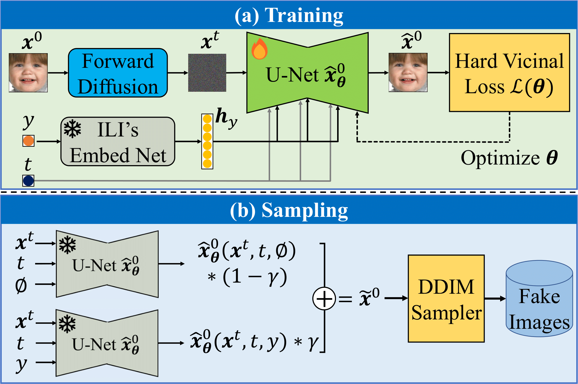
Figure 2: The overall workflow of CCDMs. The training process entails adapting a modified U-Net using the proposed hard vicinal loss and integrating CcGANs’ label embedding network, referred to as ILI. For the sampling process, a classifier-free guidance-based mechanism is employed to produce a linear combination of a conditional output and an unconditional output from the trained U-Net. A DDIM-based sampler is then used to generate new images based on this linear combination.

III-A Conditional Diffusion Processes

The proposed CCDM is a conditional diffusion model, consisting of a forward diffusion process and a reverse diffusion process. In both of these processes, we include the regression label $y$ as the condition.

III-A1 Forward Diffusion Process

Given a random sample drawn from the actual conditional distribution $\bm{x}^{0}\sim p(\bm{x}^{0}|y)$, we define a forward diffusion process by adding a small amount of Gaussian noise to the samples over $T$ steps, resulting in a Markov chain with a sequence of noisy samples $\bm{x}^{1},\ldots,\bm{x}^{T}$. All of these noisy samples should share the same regression labels $y$ and dimensions as $\bm{x}^{0}$. The state transition for this Markov chain is defined as a non-learned Gaussian model:

$$q(\bm{x}^{t}|\bm{x}^{t-1},y)=\mathcal{N}(\bm{x}^{t};\sqrt{1-\beta_{t}}\bm{x}^{t-1},\beta_{t}\bm{I})$$ (3)

where $0\leq\beta_{1}<\beta_{2}<...<\beta_{T}\leq 1$ are potentially learnable variances but fixed to constants using the cosine schedule [nichol2021improved] for simplicity. In this chain, the random sample $\bm{x}^{0}$ gradually loses its recognizable structures as $t$ increases, and eventually becomes a standard Gaussian noise when $T\rightarrow\infty$.

Let $\alpha_{t}=1-\beta_{t}$ and $\bar{\alpha}_{t}=\prod_{i=1}^{t}\alpha_{i}$, as derived by Ho et al. [ho2020denoising], we can sample $\bm{x}^{t}$ at any arbitrary time step $t$ from

$$q(\bm{x}^{t}|\bm{x}^{0},y)=\mathcal{N}(\bm{x}^{t};\sqrt{\bar{\alpha}_{t}}\bm{x}^{0},(1-\bar{\alpha}_{t})\bm{I})$$ (4)

Therefore, we have

$$\bm{x}^{t}=\sqrt{\bar{\alpha}_{t}}\bm{x}^{0}+\sqrt{1-\bar{\alpha}_{t}}\bm{\epsilon}\quad\text{where}\quad\bm{\epsilon}\sim\mathcal{N}(\bm{0},\bm{I})$$ (5)

Remark 1.

Although there is a condition $y$ in Eqs.(3) and (4), $y$ does not explicitly influence the process. The forward diffusion process is almost identical to that of DDPMs [ho2020denoising].

III-A2 Reverse Diffusion Process

In the reverse diffusion process, we aim to leverage the condition $y$ to guide the reconstruction of $\bm{x}^{0}$ from the Gaussian noise $\bm{x}^{T}\sim\mathcal{N}(\bm{0},\bm{I})$. Unfortunately, estimating $q(\bm{x}^{t-1}|\bm{x}^{t},y)$ is usually nontrivial. Nevertheless, this reversed conditional distribution is tractable when conditioned on $\bm{x}^{0}$ [luo2022understanding]:

$$q(\bm{x}^{t-1}|\bm{x}^{t},\bm{x}^{0},y)=\mathcal{N}(\bm{x}^{t-1};\bm{\mu}_{q}(\bm{x}^{t},\bm{x}^{0},y),\bm{\Sigma}_{q}(t))$$ (6)

where,

$$\tilde{\bm{\mu}}(\bm{x}^{t},\bm{x}^{0},y)=\frac{\sqrt{\alpha_{t}}(1-\bar{\alpha}_{t-1})\bm{x}^{t}+\sqrt{\bar{\alpha}_{t-1}}(1-\alpha_{t})\bm{x}^{0}}{1-\bar{\alpha}_{t}}$$ (7)

$$\bm{\Sigma}_{q}(t)=\frac{(1-\alpha_{t})(1-\bar{\alpha}_{t-1})}{1-\bar{\alpha}_{t}}\bm{I}\triangleq\sigma_{q}^{2}(t)\bm{I}$$ (8)

When generating new data points, $\bm{x}^{0}$ is inherently unknown. Therefore, we train a parametric model to approximate $q(\bm{x}^{t-1}|\bm{x}^{t},\bm{x}^{0},y)$ using the following form:

$$p_{\bm{\theta}}(\bm{x}^{t-1}|\bm{x}^{t},y)=\mathcal{N}(\bm{x}^{t-1};\bm{\mu}_{\bm{\theta}}(\bm{x}^{t},t,y),\bm{\Sigma}_{q}(t))$$ (9)

where,

$$\bm{\mu}_{\bm{\theta}}(\bm{x}^{t},t,y)$$ (10)

$$= \frac{\sqrt{\alpha_{t}}(1-\bar{\alpha}_{t-1})\bm{x}^{t}+\sqrt{\bar{\alpha}_{t-1}(1-\alpha_{t})}\hat{\bm{x}}_{\bm{\theta}}^{0}(\bm{x}^{t},t,y)}{1-\bar{\alpha}_{t}}$$ (11)

In Eq. (11), $\hat{\bm{x}}_{\bm{\theta}}^{0}(\bm{x}^{t},t,y)$ is parameterized by a denoising U-Net [ronneberger2015u, ho2020denoising], designed to predict $\bm{x}^{0}$ based on the noisy image $\bm{x}^{t}$, timestamp $t$, and condition $y$ associated with both $\bm{x}^{t}$ and $\bm{x}^{0}$, where $\bm{\theta}$ denotes the trainable parameters.

Remark 2.

We choose to use this DDPM-based formulation of diffusion processes for practical demonstration purposes, although there exist numerous alternative explanations of diffusion models, including those rooted in Stochastic Differential Equations (SDEs) [song2019generative, song2021scorebased].

III-B Denoising U-Net and Conditioning Mechanism

The network architecture of the denoising U-Net, denoted as $\hat{\bm{x}}_{\bm{\theta}}^{0}(\bm{x}^{t},t,y)$, is depicted in Fig. 3. This U-Net is derived from the CFG framework [ho2021classifier], originally designed for class-conditional generative modeling tasks. In our adaptation, we have customized the conditioning mechanism by incorporating the ILI’s label embedding network $\phi(y)$ provided by [ding2023ccgan]. The label embedding network transforms a given regression label $y$ into a vector denoted by $\bm{h}_{y}$ with a length of 128. Subsequently, the vector $\bm{h}_{y}$ is fed into an embedding block before being input into the U-Net blocks. The backbone of the U-Net comprises a stack of residual blocks and self-attention blocks, with the time embedding and condition embedding being fed into each residual block. Within each residual block, we concatenate the time and condition embedding vectors, followed by a SiLU activation [elfwing2018sigmoid] and a linear layer. The resulting outputs are transformed into the scale and shift parameters of group normalization [wu2020group], thereby enabling conditional group normalization. In contrast to DDPMs [ho2020denoising] and CFG [ho2021classifier], this U-Net is tailored to denoise input images instead of predicting the noise $\bm{\epsilon}$ in Eq. (5).

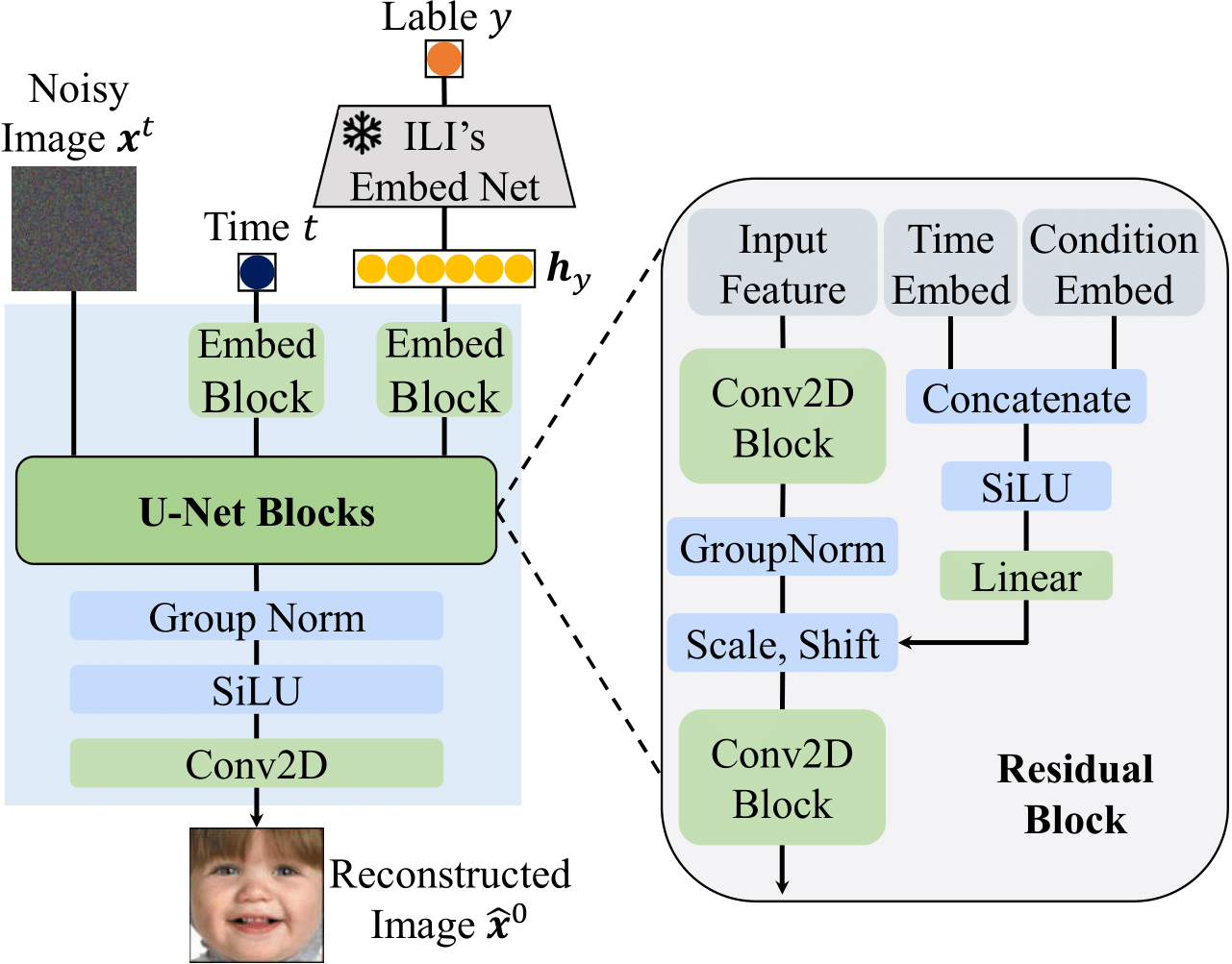
Figure 3: The network architecture of the denoising U-Net.

III-C Model Fitting Based on Vicinal Loss

The goal of CCDMs is to estimate the conditional distribution $p(\bm{x}^{0}|y)$. Typically, using $N$ image-label pairs $(\bm{x}^{0}_{1},y_{1}),...,(\bm{x}^{0}_{N},y_{N})$ for learning the trainable parameters $\bm{\theta}$, the Negative Log-Likelihood (NLL) along with its upper bound are often defined as follows:

$$-\log\mathbb{E}_{y\sim p(y)}\left[\prod_{k=1}^{N^{y}}f_{\bm{\theta}}(\bm{x}_{k,y}^{0}|y)\right]$$ (12)

$$\leq -\mathbb{E}_{y\sim p(y)}\left[\log\prod_{k=1}^{N^{y}}f_{\bm{\theta}}(\bm{x}_{k,y}^{0}|y)\right]$$ (13)

$$= \mathbb{E}_{y\sim p(y)}\left[\sum_{i=1}^{N}\mathds{1}_{\{y_{i}=y\}}\left(-\log f_{\bm{\theta}}(\bm{x}_{i}^{0}|y)\right)\right]$$ (14)

where $f_{\bm{\theta}}(\bm{x}^{0}|y)$ is the likelihood function for observed images with label $y$, $\bm{x}_{k,y}^{0}$ is the $k$-th image with label $y$, $N^{y}$ stands for the number of images with label $y$, $p(y)$ is the label distribution, and $\mathds{1}$ is the indicator function. However, Eq. (14) implies that estimating $p(\bm{x}^{0}|y)$ relies solely on images with label $y$, potentially suffering from the data insufficiency issue.

To address data sparsity, we incorporate the vicinal loss from CcGANs into the training of conditional diffusion models. Assume we use training images with labels in a hard vicinity of $y$ to estimate $p(\bm{x}^{0}|y)$, then we adjust Eq. (14) to derive the Hard Vicinal NLL (HV-NLL) as follows:

$$\mathbb{E}_{y\sim p(y)}\left[\sum_{i=1}^{N}\mathds{1}_{\{|y_{i}-y|\leq\kappa\}}\left(-\log f_{\bm{\theta}}(\bm{x}_{i}^{0}|y)\right)\right]$$ (15)

(Replace $$p(y)$$ with its kernel density estimation [silverman1986density]) (16)

$$\approx \frac{C}{N}\int\left[\sum_{i=1}^{N}\mathds{1}_{\{|y_{i}-y|\leq\kappa\}}\left(-\log f_{\bm{\theta}}(\bm{x}_{i}^{0}|y)\right)\right]$$ (17)

$$\qquad\cdot\left[\frac{1}{\sqrt{2\pi}\sigma_{\delta}}\sum_{j=1}^{N}\exp\left(-\frac{(y-y_{j})^{2}}{2\sigma_{\delta}^{2}}\right)\right]\mathrm{d}y$$ (18)

(Let $$\delta\triangleq y-y_{j} \delta\sim\mathcal{N}(0,\sigma_{\delta}^{2})$$, where ) (19)

$$= \frac{C}{N}\int\sum_{i=1}^{N}\sum_{j=1}^{N}\left[W_{h}\cdot\left(-\log f_{\bm{\theta}}(\bm{x}^{0}_{i}|y_{j}+\delta)\right)\cdot\frac{e^{-\frac{\epsilon^{2}}{2\sigma_{\delta}^{2}}}}{\sqrt{2\pi}\sigma_{\delta}}\right]\mathrm{d}\delta$$ (20)

$$= \frac{C}{N}\sum_{i=1}^{N}\sum_{j=1}^{N}\left\{\mathbb{E}_{\delta\sim\mathcal{N}(0,\sigma_{\delta}^{2})}\left[W_{h}\cdot(-\log f_{\bm{\theta}}(\bm{x}_{i}^{0}|y_{j}+\delta))\right]\right\}$$ (21)

where $C$ is a constant and

$$W_{h}\triangleq\mathds{1}_{\{|y_{j}+\delta-y_{i}|\leq\kappa\}}$$ (22)

The hard vicinal weight $W_{h}$ can alternatively be substituted with a soft vicinal weight defined by [ding2023ccgan] as follows:

$$W_{s}\triangleq\exp(-\nu(y-y^{\prime})^{2})$$ (23)

The positive hyperparameters $\kappa$, $\nu$, and $\sigma_{\delta}$ in the above formulas can be determined using guidelines outlined in [ding2023ccgan].

Eq. (21) is not analytically tractable, so instead of directly optimizing Eq.(21), we minimize its upper bound. Following the approach outlined in [ho2020denoising, luo2022understanding, murphy2023probabilistic], the key step is to derive the variational upper bound of $-\log f_{\bm{\theta}}(\bm{x}_{i}^{0}|y_{j}+\delta)$ in Eq.(21), which is expressed as follows:

$$-\log f_{\bm{\theta}}(\bm{x}_{i}^{0}|y_{j}+\delta)$$ (24)

$$\leq \mathrm{D_{KL}}(q(\bm{x}_{i}^{T}|\bm{x}_{i}^{0},y_{j}+\delta)||\mathcal{N}(\bm{0},\bm{I}))$$ (25)

$$+\sum_{t=2}^{T}\mathbb{E}_{q(\bm{x}_{i}^{t}|\bm{x}_{i}^{0},y_{j}+\delta)}\left[\mathrm{D_{KL}}(q^{t-1}||p_{\bm{\theta}}^{t-1})\right]$$ (26)

$$-\mathbb{E}_{q(\bm{x}_{i}^{1}|\bm{x}_{i}^{0},y_{j}+\delta)}\log p_{\bm{\theta}}(\bm{x}_{i}^{0}|\bm{x}_{i}^{1},y_{j}+\delta)$$ (27)

where $\mathrm{D_{KL}}(\cdot||\cdot)$ is the Kullback–Leibler divergence, and

$$q^{t-1}\triangleq q(\bm{x}_{i}^{t-1}|\bm{x}_{i}^{t},\bm{x}_{i}^{0},y_{j}+\delta)$$ (28)

$$p_{\bm{\theta}}^{t-1}\triangleq p_{\bm{\theta}}(\bm{x}_{i}^{t-1}|\bm{x}_{i}^{t},y_{j}+\delta)$$ (29)

As noted in [luo2022understanding], the summation term (Eq. (26)) dominates the reconstruction term (Eq. (27)), and Eq.(25) is a constant irrelevant to $\bm{\theta}$. Therefore, we focus solely on Eq. (26). Since both $q^{t-1}$ and $p_{\bm{\theta}}^{t-1}$ are Gaussian, as demonstrated in [luo2022understanding], $\mathrm{D_{KL}}(q^{t-1}||p_{\bm{\theta}}^{t-1})$ can be analytically computed. Moreover, [luo2022understanding] pointed out that minimizing the summation term across all noise levels in Eq. (26) can be approximated by minimizing the expectation over all time steps. Additionally, recalling that $\bm{x}^{t}=\sqrt{\bar{\alpha}_{t}}\bm{x}^{0}+\sqrt{1-\bar{\alpha}_{t}}\bm{\epsilon}$, we arrive at the following conclusions:

$$\operatornamewithlimits{arg\,min}_{\bm{\theta}}\sum_{t=2}^{T}\mathbb{E}_{q(\bm{x}_{i}^{t}|\bm{x}_{i}^{0},y_{j}+\delta)}\left[\mathrm{D_{KL}}(q^{t-1}||p_{\bm{\theta}}^{t-1})\right]$$ (30)

$$\approx \operatornamewithlimits{arg\,min}_{\bm{\theta}}\mathbb{E}_{\bm{\epsilon}\sim\mathcal{N}(\bm{0},\bm{I}),t\sim U(2,T)}\left[\lambda_{t}\right.$$ (31)

$$\qquad\left.\cdot\|\hat{\bm{x}}_{\bm{\theta}}^{0}(\sqrt{\bar{\alpha}_{t}}\bm{x}^{0}_{i}+\sqrt{1-\bar{\alpha}_{t}}\bm{\epsilon},t,y_{j}+\delta)-\bm{x}^{0}_{i}\|^{2}_{2}\right]$$ (32)

where,

$$\lambda_{t}\triangleq\frac{1}{2\sigma_{q}^{2}(t)}\frac{\bar{\alpha}_{t-1}(1-\alpha_{t})^{2}}{(1-\bar{\alpha}_{t})^{2}}$$ (33)

As empirically demonstrated by Ho et al. [ho2020denoising], setting $\lambda_{t}=1$ often leads to visually superior samples. Hence, in our training of CCDM, we have also chosen $\lambda_{t}=1$.

Building on all the above analysis, if we replace $-\log f_{\bm{\theta}}(\bm{x}_{i}^{0}|y_{j}+\delta)$ in Eq.(21) with the objective function of Eq.(32) and omit the constant $C$, the resulting simplified Hard Vicinal Loss (HVL) for training U-Net is expressed as follows:

$$\mathcal{L}(\bm{\theta}) =-\frac{1}{N}\sum_{i=1}^{N}\sum_{j=1}^{N}\left\{\mathbb{E}_{\delta\sim\mathcal{N}(0,\sigma_{\delta}^{2}),\bm{\epsilon}\sim\mathcal{N}(\bm{0},\bm{I}),t\sim U(2,T)}\left[W_{h}\vphantom{\bm{x}^{0}_{i}}\right.\right.$$ (34)

$$\left.\left.\vphantom{\mathbb{E}_{\delta\sim\mathcal{N}(0,\sigma_{\delta}^{2})}}\cdot\|\hat{\bm{x}}_{\bm{\theta}}^{0}(\sqrt{\bar{\alpha}_{t}}\bm{x}^{0}_{i}+\sqrt{1-\bar{\alpha}_{t}}\bm{\epsilon},t,y_{j}+\delta)-\bm{x}^{0}_{i}\|^{2}_{2}\right]\right\}$$ (35)

where $W_{h}$ has already been defined in Eq. (22). We also provide Algorithm 1 to describe the detailed training procedure.

Data: $N$ real image-label pairs $\Omega=\{(\bm{x}^{0}_{1},y_{1}),\dots,(\bm{x}^{0}_{N},y_{N})\}$, $N_{\text{uy}}$ distinct labels $\Upsilon=\{y_{[1]},\dots,y_{[N_{\text{uy}}]}\}$ arranged in ascending order from the training dataset;

Input: A pre-trained label embedding network $\phi(y)$ from [ding2023ccgan]; Preset hyperparameters, including the hard vicinity radius $\kappa$, the kernel density estimation variance $\sigma_{\delta}$, the total number of timesteps $T$, the probability of randomly dropping conditions $p_{\text{drop}}$, number of iterations $K$, and the batch size $m$;

Result: A trained U-Net $\hat{\bm{x}}_{\bm{\theta}}^{0}$

1 for $k=1$ to $K$ do

2       Draw $m$ regression labels, denoted by $Y$, with replacement from $\Upsilon$;

3       Create a batch of target labels $Y^{\delta}=\{y_{i}+\delta|y_{i}\in Y,\delta\in\mathcal{N}(0,\sigma_{\delta}^{2}),i=1,\dots,m\}$ ($\hat{\bm{x}}_{\bm{\theta}}^{0}$ is conditional on these labels) ;

4       Initialize $\Omega^{y_{i}+\delta}=\emptyset$ ;

5       for $i=1$ to $m$ do

6             Randomly choose an image-label pair $(\bm{x}^{0},y)\in\Omega$ satisfying $|y-y_{i}-\delta|\leq\kappa$ where $y_{i}+\delta\in Y^{\delta}$;

7             Draw $u\sim U(0,1)$;

8             if $u\geq p_{\text{drop}}$ then

9                   Update $\Omega^{y_{i}+\delta}=\Omega^{y_{i}+\delta}\cup(\bm{x}^{0},y_{i}+\delta)$;

10                  

11             else

12                   Update $\Omega^{y_{i}+\delta}=\Omega^{y_{i}+\delta}\cup(\bm{x}^{0},\emptyset)$;

13                  

14             end if

15            

16       end for

17      Convert regression labels in $\Omega^{y_{i}+\delta}$ into their multi-dimensional representation via $\phi(y)$;

18       Update $\hat{\bm{x}}_{\bm{\theta}}^{0}$ using samples in the set $\Omega^{y_{i}+\delta}$ via gradient-based optimizers according to Eq. (35);

19      

20 end for

Algorithm 1 Training Algorithm of CCDM.

Remark 3.

Since our conditional sampling technique introduced in Section III-D is derived from the classifier-free guidance proposed in [ho2021classifier], we need to implement both a conditional diffusion model and an unconditional one. Rather than training two separate models, as suggested in [ho2021classifier], we combine them into a single model by randomly converting the noisy label $y_{j}+\delta$ in Eq. (35) into $\oslash$ with probability $p_{\text{drop}}$ during training. In such instances, the conditional model $\hat{\bm{x}}_{\bm{\theta}}^{0}(\bm{x}^{t},t,y)$ is degraded to an unconditional one $\hat{\bm{x}}_{\bm{\theta}}^{0}(\bm{x}^{t},t,\oslash)$.

Remark 4.

The ablation study in Section IV demonstrates that the hard vicinal weight $W_{h}$ outperforms the soft one $W_{s}$. Therefore, we recommend utilizing $W_{h}$ in applications.

Remark 5.

As demonstrated in [ho2020denoising, luo2022understanding], Eq.(35) can be converted into the noise prediction loss (similar to Eq. (1)). However, when sampling with the accelerated sampler DDIM [song2021denoising], this noise prediction loss often results in severe label inconsistency, as shown in Section LABEL:sec:ablation.

III-D Conditional Sampling

To sample from the learned model, we adapt the CFG [dhariwal2021diffusion] framework, originally designed for class-conditional sampling, to suit the CCGM task. Suppose we intend to generate fake images conditional on a regression label $y$. Luo demonstrated in [luo2022understanding] a linear relationship between $\bm{x}^{0}$ and $\triangledown\log p(\bm{x}^{t}|y)$ as follows:

$$\bm{x}^{0}=\frac{\bm{x}^{t}+(1-\bar{\alpha}_{t})\triangledown\log p(\bm{x}^{t}|y)}{\sqrt{\bar{\alpha}_{t}}}$$ (36)

Based on Eq. (36), we modify Eq. (2) and arrive at:

$$\tilde{\bm{x}}^{0}=(1-\gamma)\cdot\underbrace{\hat{\bm{x}}_{\bm{\theta}}^{0}(\bm{x}^{t},t,\oslash)}_{\text{unconditional}}+\gamma\cdot\underbrace{\hat{\bm{x}}_{\bm{\theta}}^{0}(\bm{x}^{t},t,y)}_{\text{conditional}}$$ (37)

where the reconstructed $\bm{x}^{0}$, denoted by $\tilde{\bm{x}}^{0}$, is a linear combination of the outputs from an unconditional U-Net and a conditional U-Net. The conditional scale $\gamma$ is a hyper-parameter larger than 1.

Then, for high sampling efficiency, we employ the DDIM sampler [song2021denoising], and generate new samples with $T^{\prime}$ time steps by iteratively using the following deterministic procedure:

$$\bm{x}^{t-1}=\sqrt{\bar{\alpha}_{t-1}}\tilde{\bm{x}}^{0}+\sqrt{1-\bar{\alpha}_{t-1}}\frac{\bm{x}^{t}-\sqrt{\bar{\alpha}_{t}}\tilde{\bm{x}}^{0}}{\sqrt{1-\bar{\alpha}_{t}}}$$ (38)

Algorithm 2 is used to show the detailed sampling procedure.

Input: A pre-trained U-Net $\hat{\bm{x}}_{\bm{\theta}}^{0}$; The target regression label $y$; Preset hyperparameters, including the total number of timesteps $T^{\prime}$, the conditional scale $\gamma$, and the variance schedule $\beta_{i}$’s;

Result: A fake image $\bm{x}^{0}_{g}$ with label $y$

1 $t\leftarrow T^{\prime}$, $\bm{x}^{T^{\prime}}_{g}\sim\mathcal{N}(\bm{0},\bm{I})$;

2 while $t>0$ do

3       Compute $\alpha_{t}=1-\beta_{t}$ and $\bar{\alpha}_{t}=\prod_{i=1}^{t}\alpha_{i}$;

4       Compute $\tilde{\bm{x}}^{0}=(1-\gamma)\cdot\hat{\bm{x}}_{\bm{\theta}}^{0}(\bm{x}^{t}_{g},t,\oslash)+\gamma\cdot\hat{\bm{x}}_{\bm{\theta}}^{0}(\bm{x}^{t}_{g},t,y)$;

5       Update $\bm{x}^{t-1}_{g}=\sqrt{\bar{\alpha}_{t-1}}\tilde{\bm{x}}^{0}+\sqrt{1-\bar{\alpha}_{t-1}}\frac{\bm{x}^{t}_{g}-\sqrt{\bar{\alpha}_{t}}\tilde{\bm{x}}^{0}}{\sqrt{1-\bar{\alpha}_{t}}}$;

6       Update $t\leftarrow t-1$;

7 end while

Algorithm 2 Sampling Algorithm of CCDM.

IV Experiments

IV-A Experimental Setup

Datasets. We evaluate the effectiveness of CCDM across four datasets with varying resolutions ranging from $64\times 64$ to $192\times 192$. These datasets comprise RC-49 [ding2023ccgan], UTKFace [utkface], Steering Angle [steeringangle], and Cell-200 [ding2023ccgan]. Brief introductions to these datasets are presented below:

• RC-49: The RC-49 dataset comprises 44,051 RGB images at a resolution of $64\times 64$, representing 49 types of chairs. Each chair type includes 899 images labeled with 899 distinct yaw rotation angles ranging from $0.1^{\circ}$ to $89.9^{\circ}$, with a step size of $0.1^{\circ}$. For training purposes, we select yaw angles with odd numbers as the last digit. Subsequently, we randomly choose 25 images for each selected angle to create a training set. The final training set of RC-49 consists of 11,250 images corresponding to 450 distinct yaw angles.

• UTKFace: The UTKFace dataset consists of RGB human face images, with ages serving as regression labels. We utilize the pre-processed UTKFace dataset [ding2021ccgan], which includes 14,760 RGB images spanning ages from 1 to 60 years. The dataset features varying numbers of images per age, ranging from 50 to 1051, and all images are used for training. The UTKFace dataset is available in three versions with resolutions of $64\times 64$, $128\times 128$, and $192\times 192$.

• Steering Angle: The Steering Angle dataset originates from an autonomous driving dataset, as referenced in [steeringangle, steeringangle2]. In our experiments, we make use of a preprocessed dataset curated by Ding et al. [ding2023ccgan]. This refined dataset encompasses 12,271 RGB images labeled with 1,774 unique steering angles, ranging from $-80.0^{\circ}$ to $80.0^{\circ}$. These images were recorded using a dashboard-mounted camera in a car, capturing the corresponding steering wheel rotation angles simultaneously. The Steering Angle dataset includes two versions, with resolutions of $64\times 64$ and $128\times 128$.

• Cell-200: The Cell-200 dataset, created by Ding et al. [ding2023ccgan], contains 200,000 synthetic grayscale microscopic images, each at a resolution of $64\times 64$. Each image contains a variable number of cells, ranging from 1 to 200, with 1,000 images available for each cell count. In the training phase, we specifically select a subset of the Cell-200 dataset, which only includes images having an odd number of cells, with 10 images per cell count. This curated subset consists of 1,000 training images in total. When it comes to evaluation, we utilize all 200,000 samples from the Cell-200 dataset.

Compared Methods. In accordance with the setups described in [ding2024turning], we choose the following contemporary conditional generative models for comparison:

• Two class-conditional GANs: We select ReACGAN [kang2021rebooting] and ADCGAN [hou2022conditional] as the compared methods. Both GANs utilize state-of-the-art network architectures and training techniques, and both are conditioned on discretized regression labels.

• Two class-conditional diffusion models: For comparison, we select two classic CDMs, namely ADM-G [dhariwal2021diffusion] and Classifier-Free Guidance (CFG) [ho2021classifier], both using discretized regression labels as conditions. The reason for not including more advanced CDMs, such as stable diffusion (SD)[rombach2022high] and DiT[peebles2023scalable], in our comparison is as follows: as a proof of concept, the primary objective of this paper is to demonstrate that our modifications to the diffusion processes, U-Net architecture, conditioning mechanism, and the introduction of a new vicinal loss enable effective application of CDMs to the CCGM task. These modifications and the new vicinal loss are also applicable to state-of-the-art CDMs such as SD and DiT. However, implementing SD and DiT is computationally expensive and beyond our current computational capabilities. Therefore, we base our proposed CCDM on the DDPM [ho2020denoising] and CFG [ho2021classifier] framework. For fairness, we compare our CCDM against ADM-G and CFG, which have similar model capacities.

• Two GAN-based CCGM models: We select the state-of-the-art CcGAN (SVDL+ILI) [ding2023ccgan] and Dual-NDA [ding2024turning] for our comparisons. Note that Dual-NDA [ding2024turning] is a data augmentation strategy for CcGAN aimed at improving its visual quality and label consistency. Therefore, both CcGAN (SVDL+ILI) and Dual-NDA are based on the CcGAN framework.

• Two diffusion-based CCGM models: We include the modified CcDPM [zhao2024ccdpm] and the proposed CCDM in the comparison. CcDPM [zhao2024ccdpm] was initially designed for non-image data with multi-dimensional continuous labels, but we have adapted it for the CCGM task. Specifically, we replaced the U-Net backbone and label embedding mechanism of CcDPM with our proposed approach detailed in Section III-B. However, for implementing CcDPM, we retained the soft vicinity and noise prediction error-based loss as proposed in [zhao2024ccdpm].

Note that for the $192\times 192$ experiment, we focus exclusively on comparing the four CCGM models, including CcGAN (SVDL+ILI), Dual-NDA, CcDPM, and CCDM.

Training Setup. In the implementation of class-conditional models, we bin the regression labels of four datasets into different classes: 150 classes for RC-49, 60 classes for UTKFace, 221 classes for Steering Angle, and 100 classes for Cell-200. To facilitate comparisons, we leveraged pre-trained models provided by Ding et al.[ding2024turning] for experiments on UTKFace ($64\times 64$ and $128\times 128$) and Steering Angle ($64\times 64$ and $128\times 128$) datasets, rather than re-implementing all candidate methods (excluding CCDM). Additionally, Ding et al.[ding2023ccgan] offered pre-trained ReACGAN for RC-49 and CcGAN (SVDL+ILI) for UTKFace ($192\times 192$). Apart from these pre-trained models, we re-implemented all other candidate models for comparison. When implementing CcGAN (SVDL+ILI) and Dual-NDA on Cell-200, we use DCGAN [radford2015unsupervised] as the backbone architecture and train the CcGAN models with the vanilla cGAN loss [mirza2014conditional]. When implementing CcGAN (SVDL+ILI) and Dual-NDA on RC-49, we employ SAGAN [zhang2019self] as the backbone architecture and train the CcGAN models with the hinge loss [lim2017geometric] and DiffAugment [zhao2020differentiable]. To implement CCDM, we set $p_{\text{drop}}=0.1$ in Remark 3 and $\gamma=1.5$ in Eq. (37) for most experiments. Exception is made for UTKFace ($192\times 192$), where we increase the value of $\gamma$ to 2.0 to enhance label consistency. The total time step $T$ is fixed at 1000 during training, while the sampling time step $T^{\prime}$ varies: 100 for UTKFace ($192\times 192$) and 250 for all other experiments. The hard vicinity radius $\kappa$ and other training parameters are configured differently for each experiment. The training configurations of CcDPM closely resemble those of CCDM, except that the U-Net is trained to predict noise, and the vicinity type is soft. For detailed training setups, please refer to Section LABEL:sec:detailed_train_setups in the Appendix.

Evaluation Setup. Consistent with Ding et al. [ding2021ccgan, ding2023ccgan, ding2023efficient, ding2024turning], we generate 179,800, 60,000, 100,000, and 200,000 fake images using each candidate method in the RC-49, UTKFace, Steering Angle, and Cell-200 experiments, respectively. These generated images are then evaluated using one overall metric and three separate metrics. The overall metric employed is the Sliding Fréchet Inception Distance (SFID)[ding2023ccgan]. Additionally, we use Naturalness Image Quality Evaluator (NIQE) [mittal2012making] to assess visual fidelity, Diversity [ding2023ccgan] to evaluate image diversity, and Label Score [ding2023ccgan] to measure label consistency of the generated images. Note that the Diversity score cannot be computed for the Cell-200 dataset because the samples in this dataset do not have categorical features required for such computations. For the evaluation metrics SFID, NIQE, and Label Score, smaller values are preferred as they indicate better performance. However, for the Diversity score, larger values are desirable as they represent a greater variety in the generated samples.

IV-B Experimental Results

We conduct a performance comparison of candidate methods across seven settings involving four datasets and three resolutions, as shown in Table LABEL:tab:main_results. Some example fake images generated from candidate methods are also shown in Fig. LABEL:fig:example_fake_images. Analysis of the experimental results reveals the following findings:

• Among all settings, CCDM achieves the lowest SFID scores, indicating the best overall performance. Notably, the SFID score of CCDM in the RC-49 experiment is only half that of CcGAN and Dual-NDA, showcasing substantial improvements in image quality.

• Consistent with the findings in [ding2021ccgan, ding2023ccgan, ding2024turning], class-conditional models demonstrate significantly inferior performance when compared to CCGM. Particularly, class-conditional GANs exhibit mode collapse problems in the Cell-200 experiment and often encounter issues of label inconsistency across various settings.

• In all datasets except RC-49, CCDM shows lower NIQE scores than the baseline CcGAN (SVDL+ILI), suggesting superior visual fidelity. Even when compared to Dual-NDA, which is specifically designed to enhance the visual quality of CcGAN, CCDM still demonstrates advantages in 4 out of 7 settings.

• The Diversity scores exhibit variability without a clear consistent pattern. In certain settings, CCDM shows the highest diversity, while in others, its diversity is notably lower but still above average.

• In terms of label consistency, CCDM either outperforms or is comparable to CcGAN and Dual-NDA in the $64\times 64$ and $128\times 128$ experiments. However, in the $192\times 192$ experiment, CCDM shows some label inconsistency.

• In all settings, CCDM significantly outperforms CcDPM. Furthermore, in most settings, CcDPM performs worse than GAN-based CCGM models. Notably, CcDPM exhibits poor label consistency on RC-49, indicating its failure in this regard.

• The example fake images visualized in Fig.LABEL:fig:example_fake_images further support some of the conclusions mentioned above. Specifically, the figure clearly illustrates that CcDPM exhibits poor label consistency on the RC-49 ($64\times 64$), Cell-200 ($64\times 64$), and Steering Angle ($128\times 128$) datasets. Additionally, Fig.LABEL:fig:example_fake_images demonstrates that CCDM shows better visual quality than CcGAN (SVDL+ILI) on the UTKFace ($128\times 128$) and Steering Angle ($128\times 128$) datasets.