Enhancing Channel Estimation in Quantized Systems with a Generative Prior ††thanks: The authors acknowledge the financial support by the Federal Ministry of Education and Research of Germany in the program of “Souverän. Digital. Vernetzt.”. Joint project 6G-life, project identification number: 16KISK002.
Abstract
Channel estimation in quantized systems is challenging, particularly in low-resolution systems. In this work, we propose to leverage a Gaussian mixture model (GMM) as generative prior, capturing the channel distribution of the propagation environment, to enhance a classical estimation technique based on the expectation-maximization (EM) algorithm for one-bit quantization. Thereby, a maximum a posteriori (MAP) estimate of the most responsible mixture component is inferred for a quantized received signal, which is subsequently utilized in the EM algorithm as side information. Numerical results demonstrate the significant performance improvement of our proposed approach over both a simplistic Gaussian prior and current state-of-the-art channel estimators. Furthermore, the proposed estimation framework exhibits adaptability to higher resolution systems and alternative generative priors.
Index Terms:
Generative prior, Gaussian mixture, one-bit quantization, channel estimation, expectation-maximization.©This work has been submitted to the IEEE for possible publication. Copyright may be transferred without notice, after which this version may no longer be accessible.
I Introduction
Utilizing a generative prior for inverse problems in wireless communications has attracted considerable attention recently due to the high potential of improved estimation performance, e.g., using GMMs [1], mixture of factor analyzers (MFAs) [2], variational autoencoders (VAEs) [3], generative adversarial networks (GANs) [4], or diffusion models (DMs) [5, 6]. These works promise a significant performance improvement over classical techniques and learning-based regression neural networks (NNs) by learning the channel distribution for a whole radio propagation environment, capturing valuable prior information. A general limitation is the common assumption of infinite precision analog-to-digital converters (ADCs) at the receiver. The primary motivation for deploying low-resolution ADCs is the significant improvement in energy efficiency, particularly crucial in massive multiple-input multiple-output (MIMO) systems. However, utilizing a generative prior for low-resolution quantization at the receiver, introducing a challenging inverse problem due to the pronounced nonlinearity introduced by the low-resolution ADCs, is not very well studied.
An exception is the work in [7], where conditionally Gaussian latent generative models are utilized to parameterize a conditional Bussgang estimator. Although this work offers promising performance gains for channel estimation, it is limited by the linearity of the parameterized Bussgang estimator, based on the observation that the Bussgang estimator deteriorates from the mean square error (MSE)-optimal conditional mean estimator (CME), especially for higher dimensions [8].
A different approach was discussed in [9, 10], focusing on the MAP optimization problem instead of the minimum mean square error (MMSE) estimator, which is solved with an EM algorithm. It was shown that explicit knowledge of the prior distribution is essential, and the case of a simple Gaussian prior is discussed, leading to closed-form solutions. However, a simplistic Gaussian prior considerably underrepresents the channel distribution of a whole propagation environment.
Contributions: We propose a novel estimation framework for quantized systems, enhancing the EM algorithm from [9, 10] by utilizing a conditionally Gaussian latent model as generative prior for learning the channel distribution of a whole radio propagation environment, providing valuable information for the subsequent estimation task. Due to the conditional Gaussianity of the leveraged model, we get an analytic closed-form solution for the corresponding M-step of the EM algorithm, resulting in reduced computational complexity. While our study concentrates on a GMM as generative prior and the extreme case of one-bit quantization, the proposed estimation framework exhibits adaptability for higher resolution systems and alternative generative priors, e.g., MFAs or VAEs. We discuss different structural constraints on the covariances of the GMM, i.e., Toeplitz or circulant structure, resulting in reduced memory overhead and computational complexity. Numerical results demonstrate significant performance gains compared to using a simplistic Gaussian model as prior and state-of-the-art channel estimators in quantized systems.
Notation: The -th element of a vector is denoted as and its real and imaginary parts are given as and , respectively. The standard Gaussian cumulative distribution function (CDF) is denoted by .
II System and Channel Model
Consider an uplink transmission of pilot signals from single-antenna mobile terminals (MTs) to an -antenna base station (BS), operating one-bit ADCs. The quantized receive signal is , where , is the unquantized receive signal, denotes the wireless channel, and is the pilot vector with the entries, cf. [7], , where is the amplitude spacing. The pilot vector is subsequently normalized to fulfill the power constraint . Furthermore, is white Gaussian noise with and denotes the complex-valued one-bit quantization function
| (1) |
After column-wise vectorization, the system model is
| (2) |
with , , , and . By normalizing the channels as , the signal-to-noise ratio (SNR) is defined as .
We utilize a stochastic-geometric channel model based on the 3rd Generation Partnership Project (3GPP) spatial channel model [11, 12], where channels are modeled conditionally Gaussian: . The random vector collects the uniform distributed angles of arrival/departure and path gains of the main propagation clusters between a MT and the BS. The BS employs a uniform linear array (ULA) such that the spatial channel covariance matrix is given by
| (3) |
with being the array steering vector for an angle of arrival , and is a power density consisting of a sum of weighted Laplace densities whose standard deviations describe the angle spread of the propagation clusters [11]. To create a training dataset , we generate random angles and path gains for every data sample , combined in , and then draw the sample as , which results in an overall non-Gaussian channel distribution [9842343] of the training dataset
III EM Algorithm with a Gaussian Prior
In this section, we briefly summarize the EM algorithm for channel estimation from [9, 10], where the case of a Gaussian prior is explicitly discussed. The goal is to solve the MAP optimization problem, given as
| (4) |
However, as outlined in [9, 10], the direct optimization of \tagform@4 is intractable since the involved densities are inaccessible even under a known (Gaussian) prior. Thus, an EM algorithm is utilized, where the unquantized receive signal is considered as a latent variable. The corresponding joint likelihood is decomposed as where is an indicator function since the quantization function \tagform@1 is deterministic and . In this section, it is further assumed that the prior distribution is a zero-mean Gaussian, i.e., .
After some reformulations, the E-step of the EM algorithm in the -th iteration is shown to consist of the computation of the conditional expectation , whose real part can be computed elementwise as, cf. [9, 10],
| (5) |
where . The imaginary part is computed analogously. Although the Gaussian CDF has no analytic expression, there exist practicably feasible approximations, e.g., [13].
Furthermore, in the M-step, the updated channel estimate is computed as [10]
| (6) |
In the case of a zero-mean Gaussian prior, as discussed above, the optimization problem \tagform@6 has the closed-form analytic solution [9, 10]
| (7) |
The E- and M-steps are repeated after properly initializing until convergence.
IV Enhanced Channel Estimation with a Generative Prior
The prerequisite of the EM algorithm in Section III that the channel is Gaussian imposes a severe limitation. This becomes particularly evident when considering the channel distribution of a whole radio propagation environment, generally being considerably underrepresented by a simplistic Gaussian prior. Thus, we aim to enhance the presented EM algorithm by learning the channel distribution with a generative model, providing a much stronger prior. A variety of generative models exist for implicitly learning the channel distribution through a NN that produces valid channel samples, e.g., GANs [4] or DMs [5, 6]; however, the M-step in \tagform@6 may no longer be tractable to solve, rendering such models difficult to use.
To circumvent this problem, we resort to conditionally Gaussian latent variable models, i.e., GMMs, MFAs, or VAEs. These models facilitate the inference of a latent variable that, when conditioned on the channel distribution, produces an analytically tractable conditionally Gaussian model for the channel. In this study, our emphasis is primarily on GMMs, although the other models are, in principle, equally suitable.
A GMM is a probability density function (PDF) of the form
| (8) |
with the set of learnable parameters being the mixing coefficients, means, and covariances of the corresponding mixture components. The parameters of the GMM are fitted in an offline phase via the EM algorithm111Note that this EM algorithm has no intended connection to the presented algorithm in Section III. for a given training dataset of channel samples, cf. [14, Ch. 9]. An essential property of GMMs is that for a given data sample, the responsibility of each component can be computed as, cf. [14, Ch. 9], . The GMM can be described via a discrete latent variable with a categorical distribution, which conditions on one of the components [14, Ch. 9] and, thus, yields a conditionally Gaussian latent variable model. In [7], it was shown that a zero-mean GMM with for all is sufficient to well approximate a feasible wireless channel distribution. Since this allows for simplified expressions of the resulting algorithm, we also use a zero-mean GMM.
Directly plugging the learned GMM distribution into \tagform@5 yields no closed-form solution, requiring, e.g., a gradient descent technique. Solving this non-convex optimization problem in every iteration leads to high complexity and the possibility of reaching local minima. Thus, we instead propose to infer the most responsible GMM component for a given pilot observation and run the EM algorithm from Section III for the conditional Gaussian prior, leading to a closed-form analytic solution. An estimate of the GMM components’ responsibility for a given pilot observation from \tagform@2 can be computed as [7]
| (9) |
where is computed through with the arcsine law [15] as
| (10) |
where .
Consequently, the most responsible GMM component for a given quantized pilot observation is the MAP estimate [16]
| (11) |
When assuming the corresponding most responsible GMM component is the true prior distribution, the M-step in the -th iteration of the EM algorithm from Section III changes to
| (12) |
Due to the Gaussianity of by design, the closed form solution is given as
| (13) |
The E-step in \tagform@5 is unchanged since it does not depend on the prior distribution. The offline phase, consisting of fitting the GMM once to the underlying channel distribution of the radio propagation environment and the online evaluation of the EM algorithm, enhanced by the generative prior, is summarized in Algorithm 1, labeled GMM-EM.
IV-A Structural Constraints
To further incorporate structural properties to the generative prior, imposed by the antenna structure at the BS, i.e., Toeplitz (GMM-EM toep) or circulant (GMM-EM circ) covariances, we utilize a structured GMM as outlined in [17]. Thereby, each component’s covariance is described by the decomposition
| (14) |
where is a (oversampled) discrete Fourier transform (DFT) matrix and . These structural constraints allow for having fewer model parameters and a lower online complexity overhead of the resulting estimator due to the usage of fast Fourier transforms (FFTs).
IV-B Memory and Complexity Analysis
The number of model parameters is scaling with or for the GMM with full or structurally constrained covariances, respectively. For reducing the computational complexity, many iterative computations in Algorithm 1 can be precomputed since the GMM is fixed after the offline phase, e.g., the filter in the M-step and the inverses for evaluating the responsibilities \tagform@9. Thus, the order of complexity is dominated by matrix-vector products, yielding , where is the number of iterations of the EM algorithm until convergence. We note that the computations of the responsibilities \tagform@9 are trivially parallelizable. Although the order of complexity is the same for the structurally constrained versions, the number of floating point operations (FLOPs) is drastically reduced by using FFTs.
V Baseline Channel Estimators
In the following, we introduce several theoretical and practical state-of-the-art baselines that are most related and relevant for evaluating the estimation performance of the proposed algorithm:
-
•
genie-EM: Assuming genie-knowledge of the covariance matrix from \tagform@3 for each pilot observation allows for running the EM algorithm with the ground-truth prior by replacing with in the M-step \tagform@7. This yields a theoretical bound on the best-possible estimation performance when utilizing the EM approach.
-
•
global-EM: Since the genie-knowledge of the covariance matrix is inaccessible in a practical scenario, we additionally evaluate the EM algorithm when assuming the prior is Gaussian; thus, in this case, the sample covariance matrix of the training dataset, i.e., , is used in the M-step \tagform@7.
-
•
genie-BLMMSE: Similar to the genie-EM approach, we assume genie-knowledge of the covariance matrix from \tagform@3 for each pilot observation to evaluate a bound on the performance of the linear MMSE estimator based on the Bussgang decomposition, cf. [7].
-
•
global-BLMMSE: In this case, instead of utilizing the ground-truth covariance matrix, we utilize the sample covariance matrix for evaluating an approximation of the Bussgang linear MMSE estimator [7].
-
•
EM-GM-GAMP: In [18], a compressive sensing (CS)-based channel estimator is proposed, which is a combination of an EM algorithm for approximating the channel PDF in the (approximately) sparse angular domain and the generalized approximate message passing (GAMP) algorithm to solve the sparse recovery problem.
-
•
GMM-BLMMSE: We additionally compare to the parameterized conditional Bussgang estimator based on the GMM from [7]. Note that learning the channel distribution via a GMM is similar to the proposed approach; however, we do not parameterize a linear MMSE estimator.
VI Numerical Results
For all data-aided approaches, we utilize the same training dataset consisting of data samples. As performance measure we evaluate an estimate of the normalized MSE using unseen channel samples. If not otherwise stated, we utilize a GMM with full covariances. We set and .
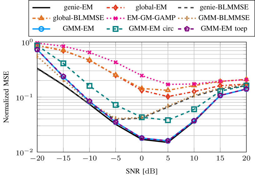
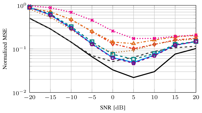
Fig. 1 evaluates the MSE performance over the SNR for one (top) and three (bottom) propagation clusters with antennas and pilot observations. It can be observed that genie-EM outperforms genie-BLMMSE, indicating that the MAP objective is superior over the linear MMSE estimator based on the Bussgang decomposition, especially in the medium to high SNR regime. This observation is in accordance with the finding in [8] that the Bussgang estimator significantly deteriorates from the CME in general, justifying the adoption of nonlinear estimation approaches. The proposed GMM-EM is on par with the related GMM-BLMMSE in the low SNR regime; however, in medium and high SNR, it exhibits a significant performance improvement, even outperforming the genie-BLMMSE approach, which requires genie knowledge of the true covariance matrix for each observation. Moreover, all other state-of-the-art estimators are outperformed with a large gap over the whole range of SNR. In the case of one propagation cluster, the proposed GMM-EM approach even reaches the performance of genie-EM. In contrast, the gap is generally higher for more propagation clusters where the channel distribution is less structured. The Toeplitz-structured GMM is on par with the full GMM, whereas there is a larger gap for the circulant case, imposing a stronger approximation.
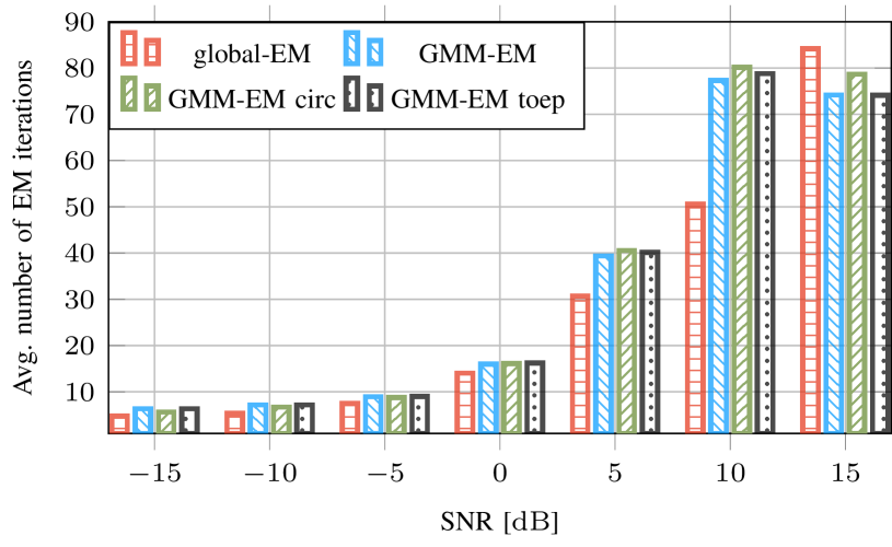
In Fig. 2, we analyze the necessary number of EM iterations until convergence for the setup of one propagation cluster in Fig. 1. The number of iterations is particularly low in the low SNR regime, i.e., below ten iterations, for all considered variants utilizing the EM algorithm. This is a convenient property since the considered operating range of low-resolution systems is the low SNR regime where the capacity is not severely reduced [19].
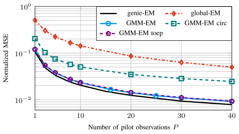
Fig. 3 investigates the MSE performance for a varying number of pilot observations for antennas and an SNR of . Since the EM-GM-GAMP is consistently worse than global-EM, and GMM-BLMMSE suffers from a too high complexity in the large pilot regime, we leave out these comparisons. It can be observed that the proposed GMM-EM approach is almost on par with the genie-aided variant over the whole range. In conclusion, the number of pilots can be drastically reduced when using the proposed approach compared to a simplistic Gaussian prior without performance losses. This, in turn, results in an increased data rate, better energy efficiency, and a lower latency of the channel estimation.
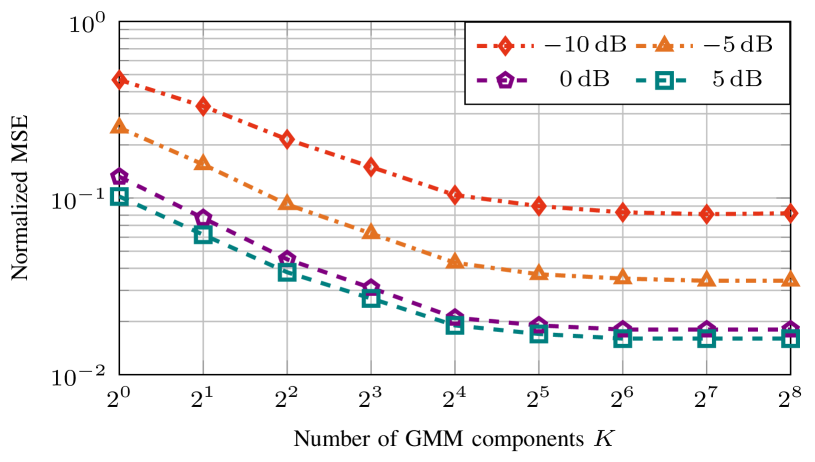
Finally, Fig. 4 evaluates the MSE performance for varying numbers of GMM components of the GMM-EM approach for one propagation cluster, antennas, and pilot observations. The performance drastically improves from (equal to the global-EM variant) to . Afterward, a saturation occurs where even more GMM components only lead to marginal improvements.
VII Conclusion and Outlook
We have presented a framework for significantly enhancing a classical channel estimation algorithm for quantized systems based on a conditionally Gaussian latent generative prior, i.e., a GMM. Inferring the component with the highest responsibility for a given pilot observation allows for having a strong prior together with a low-complexity implementation due to closed-form analytic solutions of the involved optimization problems of the EM algorithm. Furthermore, we outlined how structurally constrained GMM covariances reduce the memory and complexity overhead.
In future work, we aim to extend the presented framework to higher resolution quantization [9] and different generative priors based on conditionally Gaussian latent models, e.g., VAEs and MFAs. Additionally, we consider learning the generative prior from quantized pilot observations as training data [7].
References
- [1] M. Koller, B. Fesl, N. Turan, and W. Utschick, “An asymptotically MSE-optimal estimator based on Gaussian mixture models,” IEEE Trans. Signal Process., vol. 70, pp. 4109–4123, 2022.
- [2] B. Fesl, N. Turan, and W. Utschick, “Low-rank structured MMSE channel estimation with mixtures of factor analyzers,” in 57th Asilomar Conf. Signals, Syst., Comput., 2023, pp. 375–380.
- [3] M. Baur, B. Fesl, and W. Utschick, “Leveraging variational autoencoders for parameterized MMSE estimation,” 2024, arXiv preprint: 2307.05352.
- [4] E. Balevi, A. Doshi, A. Jalal, A. Dimakis, and J. G. Andrews, “High dimensional channel estimation using deep generative networks,” IEEE J. Sel. Areas Commun., vol. 39, no. 1, pp. 18–30, 2021.
- [5] M. Arvinte and J. I. Tamir, “MIMO channel estimation using score-based generative models,” IEEE Trans. Wireless Commun., vol. 22, no. 6, pp. 3698–3713, 2023.
- [6] B. Fesl, M. Baur, F. Strasser, M. Joham, and W. Utschick, “Diffusion-based generative prior for low-complexity MIMO channel estimation,” 2024, arXiv preprint: 2307.05352.
- [7] B. Fesl, N. Turan, B. Böck, and W. Utschick, “Channel estimation for quantized systems based on conditionally Gaussian latent models,” IEEE Trans. Signal Process., vol. 72, pp. 1475–1490, 2024.
- [8] B. Fesl, M. Koller, and W. Utschick, “On the mean square error optimal estimator in one-bit quantized systems,” IEEE Trans. Signal Process., vol. 71, pp. 1968–1980, 2023.
- [9] A. Mezghani, F. Antreich, and J. A. Nossek, “Multiple parameter estimation with quantized channel output,” in Int. ITG Workshop Smart Antennas (WSA), 2010, pp. 143–150.
- [10] C. Stöckle, J. Munir, A. Mezghani, and J. A. Nossek, “Channel estimation in massive MIMO systems using 1-bit quantization,” in IEEE 17th Int. Workshop Signal Process. Advances Wireless Commun. (SPAWC), 2016.
- [11] 3GPP, “Spatial channel model for multiple input multiple output (MIMO) simulations,” 3rd Generation Partnership Project (3GPP), Tech. Rep. 25.996 (V16.0.0), Jul. 2020.
- [12] D. Neumann, T. Wiese, and W. Utschick, “Learning the MMSE channel estimator,” IEEE Trans. Signal Process., vol. 66, no. 11, pp. 2905–2917, Jun. 2018.
- [13] P. Borjesson and C.-E. Sundberg, “Simple approximations of the error function Q(x) for communications applications,” IEEE Trans. Commun., vol. 27, no. 3, pp. 639–643, 1979.
- [14] C. M. Bishop, Pattern Recognition and Machine Learning (Information Science and Statistics). Springer New York, 2006.
- [15] G. Jacovitti and A. Neri, “Estimation of the autocorrelation function of complex Gaussian stationary processes by amplitude clipped signals,” IEEE Trans. Inf. Theory, vol. 40, no. 1, pp. 239–245, 1994.
- [16] N. Turan, B. Fesl, M. Koller, M. Joham, and W. Utschick, “A versatile low-complexity feedback scheme for FDD systems via generative modeling,” IEEE Trans. Wireless Commun., pp. 1–1, 2023.
- [17] B. Fesl, M. Joham, S. Hu, M. Koller, N. Turan, and W. Utschick, “Channel estimation based on Gaussian mixture models with structured covariances,” in 56th Asilomar Conf. Signals, Syst., Comput., 2022, pp. 533–537.
- [18] J. Mo, P. Schniter, and R. W. Heath, “Channel estimation in broadband millimeter wave MIMO systems with few-bit ADCs,” IEEE Trans. Signal Process., vol. 66, no. 5, pp. 1141–1154, 2018.
- [19] J. A. Nossek and M. T. Ivrlač, “Capacity and coding for quantized MIMO systems,” in Proc. Int. Conf. Wireless Commun. Mobile Comput., 2006, p. 1387–1392.