Asymptotic-preserving hybridizable discontinuous Galerkin method for the Westervelt quasilinear wave equation

Abstract

We discuss the asymptotic-preserving properties of a hybridizable discontinuous Galerkin method for the Westervelt model of ultrasound waves. More precisely, we show that the proposed method is robust with respect to small values of the sound diffusivity damping parameter $\delta$ by deriving low- and high-order energy stability estimates, and a priori error bounds that are independent of $\delta$. Such bounds are then used to show that, when $\delta\rightarrow 0^{+}$, the method remains stable and the discrete acoustic velocity potential $\psi_{h}^{(\delta)}$ converges to $\psi_{h}^{(0)}$, where the latter is the singular vanishing dissipation limit. Moreover, we prove optimal convergence for the approximation of the acoustic particle velocity variable $\underaccent{\bar}{\boldsymbol{v}}=\nabla\psi$. The established theoretical results are illustrated with some numerical experiments.

Keywords: asymptotic-preserving method, nonlinear acoustics, Westervelt equation, hybridizable discontinuous Galerkin method.

Mathematics Subject Classification. 65M60, 65M15, 35L70.

1 Introduction

Let $Q_{T}=\Omega\times(0,T)$ be a space–time cylinder, where $\Omega\subset\mathbb{R}^{d}$ $(d\in\{2,3\})$ is an open, bounded polytopic domain with Lipschitz boundary $\partial\Omega$, and $T>0$ is the final time. We consider the following Westervelt equation of nonlinear acoustics [36]:

$$\begin{cases}(1+2k\partial_{t}{\psi})\partial_{tt}{\psi}-c^{2}\Delta\psi-\delta\Delta(\partial_{t}{\psi})=0&\text{ in }Q_{T},\\ \psi=0&\text{ on }\partial\Omega\times(0,T),\\ \psi=\psi_{0},\qquad\partial_{t}\psi=\psi_{1}&\text{ on }\Omega\times\{0\},\end{cases}$$ (1.1)

where the unknown $\psi:Q_{T}\rightarrow\mathbb{R}$ is the acoustic velocity potential. In IBVP (1.1), the constant $k\in\mathbb{R}$ is a medium-dependent nonlinearity parameter, $c>0$ is the speed of sound, $\psi_{0}$ and $\psi_{1}$ are given initial data, and $\delta\geq 0$ is the sound diffusivity coefficient.

Introducing the acoustic particle velocity variable $\underaccent{\bar}{\boldsymbol{v}}:Q_{T}\rightarrow\mathbb{R}^{d}$, defined by $\underaccent{\bar}{\boldsymbol{v}}:=\nabla\psi$, the Westervelt equation in (1.1) can be rewritten in mixed form as

$$\begin{cases}(1+2k\partial_{t}{\psi})\partial_{tt}{\psi}-c^{2}\nabla\cdot\underaccent{\bar}{\boldsymbol{v}}-\delta\nabla\cdot(\partial_{t}\underaccent{\bar}{\boldsymbol{v}})=0&\text{ in }Q_{T},\\ \underaccent{\bar}{\boldsymbol{v}}=\nabla\psi&\text{ in }Q_{T},\\ \psi=0&\text{ on }\partial\Omega\times(0,T),\\ \psi=\psi_{0},\qquad\partial_{t}\psi=\psi_{1}&\text{ on }\Omega\times\{0\}.\end{cases}$$ (1.2)

Since we study the limit as $\delta\to 0^{+}$, we make the purely technical assumption that $\delta\in[0,\overline{\delta})$ for some fixed $\overline{\delta}>0$. Such an assumption is helpful in the limiting behavior analysis in Section 5, as it allows us to make the estimates depend on $\overline{\delta}$ but never on $\delta$ itself.

The Westervelt equation in (1.1) models the propagation of sound in a fluid medium, and it is a well-accepted model in nonlinear acoustics (see e.g., [22, §5.3]). Nonlinear sound propagation finds a multitude of technical and medical applications, such as ultrasound imaging, lithotripsy, welding, and sonochemistry; see [12, 23].

When the parameter $\delta$ is strictly positive, equation (1.1) is strongly damped, and its solution enjoys global existence properties for initial conditions satisfying some smallness and regularity assumptions as shown in [18, 30]. Conversely, when $\delta=0$, the main mechanism preventing the formation of singularities is lost and no global existence results are known. The stark contrast between these two regimes gives rise to interesting issues, such as the continuous dependence of the solution on the damping parameter $\delta\to 0^{+}$, and the interplay of this limit and numerical discretizations. A numerical method for the Westervelt equation is said to be asymptotic preserving if it allows for interchanging the vanishing limits of the mesh size parameter $h$ and the sound diffusivity parameter $\delta$, i.e., if it satisfies the commutative diagram in Figure 1. The main focus of this work is to show that the proposed method is asymptotic preserving.

Figure 1: Asymptotic-preserving commutative diagram for the Westervelt equation. This diagram represents the connections between $\psi_{h}^{(\delta)}$ and $\psi^{(\delta)}$ as $h\rightarrow 0^{+}$ (even in the limit case $\delta=0$) as well as between $\psi_{h}^{(\delta)}$ and $\psi_{h}^{(0)}$ as $\delta\to 0^{+}$. The superscript $(\delta)$ is used to emphasize the dependence on the parameter $\delta$ of the continuous solution and its numerical approximation.

In the literature, a priori error results for the approximation of the Westervelt equation initially relied on the assumption of strictly positive values of the damping parameter $\delta$ (see, e.g., [33, 2]). Nevertheless, as the damping parameter is relatively small in practice and it can become negligible in certain applications, there have been recent efforts to devise numerical methods that are robust with respect to small values of the sound diffusivity parameter $\delta$. In particular, estimates for the standard and mixed finite element discretizations of the Westervelt equation with $\delta=0$ follow as particular cases of those in [16, 26, 29], whereas the asymptotic behaviour of such methods for $\delta\rightarrow 0^{+}$ has been recently studied in [32, 14]. The main challenge resides in the limited regularity offered by most standard finite element spaces, which hinders the extension of the arguments used to study the vanishing viscosity limit in the continuous setting (see, e.g., [20]).

This work concerns the asymptotic analysis of a hybridizable discontinuous Galerkin (HDG) method for the Westervelt equation when $\delta\to 0^{+}$. HDG methods, originally introduced in [7] for an elliptic PDE, are a class of discontinuous Galerkin methods characterized by the possibility of performing a local static condensation procedure to reduce the number of unknowns of the linear system stemming from the discretization of a $d$-dimensional linear PDE. Such a procedure leads to a linear systems involving only unknowns associated with degrees of freedom on $(d-1)$-dimensional mesh-facets. Although this hybridization property does not naturally extend to nonlinear PDEs, it can be used in combination with suitable nonlinear solvers (see, e.g., Section 6.1 below). Moreover, provided that the exact solution is smooth enough, the Local Discontinuous Galerkin-hybridizible (LDG-H) method in [4, 7] for the Poisson equation converges with optimal order $\mathcal{O}(h^{p+1})$ for the $L^{2}(\Omega)$-error of the flux variable when approximations of degree $p$ are used, and allows for a local postprocessing that produces an approximation of degree $p+1$ of the primal variable that superconverges with order $\mathcal{O}(h^{p+2})$ in the $L^{2}(\Omega)$-norm.

To the best of our knowledge, there are four different versions of the HDG method for the linear acoustic wave equation $(c^{-2}\partial_{tt}u-\Delta u=f)$:

1. the dissipative HDG method introduced in [31] and analyzed in [11], which is based on the first-order system $(\partial_{t}\underaccent{\bar}{\boldsymbol{q}}=\nabla v;\ c^{-2}\partial_{t}v-\nabla\cdot\underaccent{\bar}{\boldsymbol{q}}=f)$ with $v:=\partial_{t}u$ and $\underaccent{\bar}{\boldsymbol{q}}:=\nabla u$;

2. the conservative HDG method in [15] based on the same first-order system, whose energy conserving property is enforced by choosing the numerical fluxes of $\underaccent{\bar}{\boldsymbol{q}}_{h}$ in dependence of $\partial_{t}v_{h}$, which in turn causes a theoretical loss of convergence of half an order;

3. the HDG method in [34] for the Hamiltonian formulation $(\partial_{t}u=v;\ c^{-2}\partial_{t}v=f+\nabla\cdot\underaccent{\bar}{\boldsymbol{q}})$; and

4. the conservative HDG method in [6], which is based on the mixed formulation $(\underaccent{\bar}{\boldsymbol{q}}=-\nabla u;\ c^{-2}\partial_{tt}u+\nabla\cdot\underaccent{\bar}{q}=f)$.

The theoretical results in a), c), and d) predict optimal convergence for the approximation of all the variables involved, and superconvergence for some (locally computable) postprocessed approximations of the scalar variables.

In this work, we design a HDG method for the Westervelt model, which is based on the conservative HDG method in [6] for the linear second-order wave equation. This choice allows us to directly approximate the variables of interest $(\psi,\underaccent{\bar}{\boldsymbol{v}})$, eliminate efficiently the discrete vector variable $\underaccent{\bar}{\boldsymbol{v}}_{h}$ from the nonlinear ODE system, and obtain optimal convergence in the low- and high-order energy norms. Moreover, it facilitates the extension of the techniques used for the analysis of mixed FEM discretizations of the Westervelt equation [29].

Main contributions.

The main theoretical results in this work are as follows: under some sensible assumptions on the smallness and regularity of the exact solution, we show that

1. There exists a unique solution to the proposed HDG semi-discrete formulation.

2. Optimal convergence rates of order $\mathcal{O}(h^{p+1})$ are achieved for the error of the method in some energy norms. In particular, the higher accuracy obtained for the approximation of the acoustic particle velocity $\underaccent{\bar}{\boldsymbol{v}}$ exceeds the one expected for standard DG discretizations; cf. [2]. An accurate numerical approximation of $\underaccent{\bar}{\boldsymbol{v}}$ is relevant, e.g., for enforcing absorbing conditions [35] or gradient-based shape optimization of focused ultrasound devices [21, 28].

3. The method is asymptotic preserving (i.e., the commutative diagram in Figure 1 holds), which implies that the semi-discrete approximation does not degenerate when $\delta\to 0^{+}$.

These theoretical results are validated in Section 6 below by some numerical examples. In addition, we numerically observe superconvergence of the discrete approximation of $\psi$ obtained by the local postprocessing technique in [6, Eq. (2.2)].

Outline of the paper.

In Section 2, we introduce the discrete spaces and the HDG semi-discrete formulation for model (1.2). In Section 3, we study the well-posedness and derive a priori error estimates for an auxiliary linearized problem. By means of a fixed-point argument, such results are extended in Section 4 to the nonlinear Westervelt equation. Section 5 is devoted to establishing the convergence of the numerical scheme to its vanishing $\delta$-limit. In Section 6, we describe a fully discrete scheme obtained by combining the proposed HDG method with a predictor-corrector Newmark time discretization, and illustrate our theoretical findings with some numerical experiments. We end this work with some concluding remarks in Section 7.

Notation.

We denote the first, second, and third, partial derivatives with respect to the time variable $t$ of a function $v$ by $\partial_{t}{v}$, $\partial_{tt}{v}$, and $\partial_{ttt}{v}$, respectively.

We shall use the notation $x\lesssim y$, which stands for $x\leq Cy$, where $C$ is a generic constant that does not depend on the mesh size parameter $h$ nor on the sound diffusivity parameter $\delta$.

Standard notation for $L^{p}$, Sobolev, and Bochner spaces is employed throughout. For example, for a given bounded, Lipschitz domain $D\subset\mathbb{R}^{d}$ ($d\in\mathbb{N}$) and $s\in\mathbb{R}^{+}$, the Sobolev space $H^{s}(D)$ is endowed with the standard inner product $(\cdot,\cdot)_{s,D}$, the semi-norm $|\cdot|_{H^{s}(D)}$, and the norm $\|\cdot\|_{H^{s}(D)}$. Let $n\in\mathbb{N}$, $p\in[1,\infty]$, and $X$ be a Banach space, and denote by $\partial_{t}^{i}$ the $i$th partial derivative with respect to time. The Bochner space

$$W^{n,p}(0,T;X):=\{u\in L^{p}(0,T;X),\quad\partial_{t}^{i}u\in L^{p}(0,T;X)\quad\forall i\leq n\}$$

is endowed with the norm

$$\|u\|_{H^{n}(0,T;X)}:=\sum_{i=0}^{n}\|\partial_{t}^{i}u\|_{L^{p}(0,T;X)}\qquad\text{for all }u\in H^{n}(0,T;X).$$

2 Semi-discrete HDG formulation

Let $\{\mathcal{T}_{h}\}_{h>0}$ be a family of conformal simplicial meshes for the domain $\Omega$ satisfying the standard shape-regularity and quasi-uniformity conditions. We denote by $\mathcal{F}_{h}=\mathcal{F}_{h}^{\mathcal{I}}\cup\mathcal{F}_{h}^{\mathcal{D}}$ the set of mesh facets of $\mathcal{T}_{h}$, where $\mathcal{F}_{h}^{\mathcal{I}}$ and $\mathcal{F}_{h}^{\mathcal{D}}$ are the sets of internal and Dirichlet boundary facets, respectively. For each element $K\in\mathcal{T}_{h}$, we denote by $(\partial K)^{\circ}$ and $(\partial K)^{\mathcal{D}}$ the union of the facets of $K$ that belong to $\mathcal{F}_{h}^{\mathcal{I}}$ and $\mathcal{F}_{h}^{\mathcal{D}}$, respectively. Denoting the diameter of each element $K$ by $h_{K}$, we define the mesh size $h:=\max_{K\in\mathcal{T}_{h}}h_{K}$.

Given $p\in\mathbb{N}$, we define the following piecewise polynomial spaces

$$\mathcal{S}_{h}^{p}:=\prod_{K\in\mathcal{T}_{h}}\mathbb{P}^{p}(K),\qquad\boldsymbol{\mathcal{Q}}_{h}^{p}:=\prod_{K\in\mathcal{T}_{h}}\mathbb{P}^{p}(K)^{d},\qquad\mathcal{M}_{h}^{p}:=\prod_{F\in\mathcal{F}_{h}^{\mathcal{I}}}\mathbb{P}^{p}(F),$$ (2.1)

where $\mathbb{P}^{p}(K)$ and $\mathbb{P}^{p}(F)$ denote the spaces of polynomials of total degree at most $p$ on $K$ and $F$, respectively. We denote by $\left\llbracket\cdot\right\rrbracket_{\sf{N}}$ the normal jump operator, which is defined for all $w_{h}\in\mathcal{S}_{h}^{p}$ and $\underaccent{\bar}{\boldsymbol{r}}_{h}\in\boldsymbol{\mathcal{Q}}_{h}^{p}$ as

\displaystyle\begin{cases}\begin{tabular}[]{ll}$\left\llbracket w_{h}\right\rrbracket_{\sf{N}}:=w_{h}{}_{|_{K_{1}}}\underaccent{\bar}{\mathbf{n}}_{K_{1}}+w_{h}{}_{|_{K_{2}}}\underaccent{\bar}{\mathbf{n}}_{K_{2}}$&\hbox{\multirowsetup on\leavevmode\nobreak\ $F=\partial K_{1}\cap\partial K_{2}\in\mathcal{F}_{h}^{\mathcal{I}},\text{ for some }K_{1},K_{2}\in\mathcal{T}_{h}$,}\\ $\left\llbracket\underaccent{\bar}{\boldsymbol{r}}_{h}\right\rrbracket_{\sf{N}}:=\underaccent{\bar}{\boldsymbol{r}}_{h}{}_{|_{K_{1}}}\cdot\underaccent{\bar}{\mathbf{n}}_{K_{1}}+\underaccent{\bar}{\boldsymbol{r}}_{h}{}_{|_{K_{2}}}\cdot\underaccent{\bar}{\mathbf{n}}_{K_{2}}$\end{tabular}\end{cases}

:=⟦¯rh⟧N+¯rh⋅|K1¯nK1¯rh⋅|K2¯nK2

where $\underaccent{\bar}{\mathbf{n}}_{K}$ denotes the outward-pointing unit normal vector on $\partial K$. For any positive real number $s$, we define the following broken Sobolev space

$$H^{s}(\mathcal{T}_{h}):=\{v\in L^{2}(\Omega)\ :\ v_{|_{K}}\in H^{s}(K)\ \forall K\in\mathcal{T}_{h}\}.$$

The proposed hybridizable discontinuous Galerkin semi-discrete formulation for the Westervelt equation in (1.2) is: for all $t\in(0,T]$, find $(\psi_{h}(\cdot,t),\underaccent{\bar}{\boldsymbol{v}}_{h}(\cdot,t),\lambda_{h}(\cdot,t))\in(\mathcal{S}_{h}^{p},\boldsymbol{\mathcal{Q}}_{h}^{p},\mathcal{M}_{h}^{p})$ such that the following equations are satisfied for all $K\in\mathcal{T}_{h}$

$$\int_{K}\underaccent{\bar}{\boldsymbol{v}}_{h}\cdot\underaccent{\bar}{\boldsymbol{r}}_{h}\text{d}\boldsymbol{x}=\int_{\partial K}\widehat{\psi}_{h}\underaccent{\bar}{\boldsymbol{r}}_{h}\cdot\underaccent{\bar}{\mathbf{n}}_{K}\text{d}S-\int_{K}\psi_{h}\nabla\cdot\underaccent{\bar}{\boldsymbol{r}}_{h}\text{d}\boldsymbol{x} \qquad\forall\underaccent{\bar}{\boldsymbol{r}}_{h}\in\boldsymbol{\mathcal{Q}}_{h}^{p},$$ (2.2a)

$$\begin{split}\int_{K}(1+2k\partial_{t}{\psi}_{h})\partial_{tt}{\psi}_{h}w_{h}\text{d}\boldsymbol{x}-\int_{\partial K}w_{h}(c^{2}\widehat{\vphantom{\rule{1.0pt}{5.50005pt}}\smash{\widehat{\underaccent{\bar}{\boldsymbol{v}}}}}_{h}+\delta\partial_{t}\widehat{\vphantom{\rule{1.0pt}{5.50005pt}}\smash{\widehat{\underaccent{\bar}{\boldsymbol{v}}}}}_{h})\cdot\underaccent{\bar}{\mathbf{n}}_{K}\text{d}S\\ +\int_{K}(c^{2}\underaccent{\bar}{\boldsymbol{v}}_{h}+\delta\partial_{t}{\underaccent{\bar}{\boldsymbol{v}}}_{h})\cdot\nabla w_{h}\text{d}\boldsymbol{x}=0&\qquad\forall w_{h}\in\mathcal{S}_{h}^{p},\end{split}$$ (2.2b)

the following compatibility equation is satisfied for all $$F\in\mathcal{F}_{h}^{\mathcal{I}}$$

$$\int_{F}\mu_{h}\left\llbracket\widehat{\vphantom{\rule{1.0pt}{5.50005pt}}\smash{\widehat{\underaccent{\bar}{\boldsymbol{v}}}}}_{h}\right\rrbracket_{\sf{N}}\text{d}S=0\qquad\forall\mu_{h}\in\mathcal{M}_{h}^{p},$$ (2.2c)

and appropriate discrete initial conditions, which will be specified in Section 3.3, are prescribed.

The numerical fluxes $\widehat{\psi}_{h}$ and $\widehat{\vphantom{\rule{1.0pt}{5.50005pt}}\smash{\widehat{\underaccent{\bar}{\boldsymbol{v}}}}}_{h}$ are approximations of the traces of $\psi_{h}$ and $\underaccent{\bar}{\boldsymbol{v}}_{h}$ on $\mathcal{F}_{h}$, and are defined as follows (see [9, §3.2]):

$$\widehat{\psi}_{h}:=\begin{cases}\lambda_{h}&\text{ if }F\in\mathcal{F}_{h}^{\mathcal{I}},\\ 0&\text{ if }F\in\mathcal{F}_{h}^{\mathcal{D}},\end{cases}\qquad\widehat{\vphantom{\rule{1.0pt}{5.50005pt}}\smash{\widehat{\underaccent{\bar}{\boldsymbol{v}}}}}_{h}:=\begin{cases}\underaccent{\bar}{\boldsymbol{v}}_{h}-\tau(\psi_{h}-\lambda_{h})\underaccent{\bar}{\mathbf{n}}_{K}&\text{ if }F\in\mathcal{F}_{h}^{\mathcal{I}},\\ \underaccent{\bar}{\boldsymbol{v}}_{h}-\tau\psi_{h}\underaccent{\bar}{\mathbf{n}}_{\Omega}&\text{ if }F\in\mathcal{F}_{h}^{\mathcal{D}},\end{cases}$$ (2.3)

for some piecewise constant function $\tau$ that is double valued on $\mathcal{F}_{h}^{\mathcal{I}}$ and single valued on $\mathcal{F}_{h}^{\mathcal{D}}$. In particular, we consider the single-facet choice introduced in [4, Eq. (1.6)], i.e., given a strictly positive constant $\bar{\tau}$, we define $\tau$ on each element $K\in\mathcal{T}_{h}$ as

$$\tau{}_{|_{\partial K}}:=\begin{cases}0&\text{ on }\partial K\backslash F_{K}^{\tau},\\ \bar{\tau}&\text{ on }F_{K}^{\tau},\end{cases}$$ (2.4)

for a fixed facet $F_{K}^{\tau}$ of $K$. The compatibility condition in (2.2c) implies that the normal component of $\widehat{\vphantom{\rule{1.0pt}{5.50005pt}}\smash{\widehat{\underaccent{\bar}{\boldsymbol{v}}}}}_{h}$ is single valued on the mesh skeleton, i.e., $\left\llbracket\widehat{\vphantom{\rule{1.0pt}{5.50005pt}}\smash{\widehat{\underaccent{\bar}{\boldsymbol{v}}}}}_{h}\right\rrbracket_{\sf{N}}=0$ on $\mathcal{F}_{h}^{\mathcal{I}}$.

We define the following inner products:

$$\begin{split}(u,v)_{0,\mathcal{T}_{h}}&:=\sum_{K\in\mathcal{T}_{h}}(u,v)_{0,K},\ \ \qquad\qquad(u,v)_{0,\partial\mathcal{T}_{h}}:=\sum_{K\in\mathcal{T}_{h}}(u,v)_{0,\partial K},\\ (u,v)_{0,(\partial\mathcal{T}_{h})^{\circ}}&:=\sum_{K\in\mathcal{T}_{h}}(u,v)_{0,(\partial K)^{\circ}},\qquad(u,v)_{0,(\partial\mathcal{T}_{h})^{\mathcal{D}}}:=\sum_{K\in\mathcal{T}_{h}}(u,v)_{0,(\partial K)^{\mathcal{D}}}.\end{split}$$

Given bases for the spaces in (2.1), let $M$, $\boldsymbol{M}$, $B$, $S$, $E$, $F$, and $G$ be the matrix representations of the following bilinear forms

$$m_{h}(\psi_{h},w_{h}) :=(\psi_{h},w_{h})_{0,\mathcal{T}_{h}} \forall\psi_{h},w_{h}\in\mathcal{S}_{h}^{p},$$

$$\boldsymbol{m}_{h}(\underaccent{\bar}{\boldsymbol{v}}_{h},\underaccent{\bar}{\boldsymbol{r}}_{h}) :=(\underaccent{\bar}{\boldsymbol{v}}_{h},\underaccent{\bar}{\boldsymbol{r}}_{h})_{0,\mathcal{T}_{h}} \forall\underaccent{\bar}{\boldsymbol{v}}_{h},\underaccent{\bar}{\boldsymbol{r}}_{h}\in\boldsymbol{\mathcal{Q}}_{h}^{p},$$

$$b_{h}(\psi_{h},\underaccent{\bar}{\boldsymbol{r}}_{h}) :=(\psi_{h},\nabla\cdot\underaccent{\bar}{\boldsymbol{r}}_{h})_{0,\mathcal{T}_{h}} \forall(\psi_{h},\underaccent{\bar}{\boldsymbol{r}}_{h})\in(\mathcal{S}_{h}^{p},\boldsymbol{\mathcal{Q}}_{h}^{p}),$$

$$s_{h}(\psi_{h},w_{h}) :=(\tau\psi_{h},w_{h})_{0,\partial\mathcal{T}_{h}} \forall\psi_{h},w_{h}\in\mathcal{S}_{h}^{p},$$

$$e_{h}(\lambda_{h},\underaccent{\bar}{\boldsymbol{r}}_{h}) :=-(\lambda_{h},\left\llbracket\underaccent{\bar}{\boldsymbol{r}}_{h}\right\rrbracket_{\sf{N}})_{0,\mathcal{F}_{h}^{\mathcal{I}}} \forall(\lambda_{h},\underaccent{\bar}{\boldsymbol{r}}_{h})\in(\mathcal{M}_{h}^{p},\boldsymbol{\mathcal{Q}}_{h}^{p}),$$

$$f_{h}(\lambda_{h},w_{h}) :=-(\tau\lambda_{h},w_{h})_{0,(\partial\mathcal{T}_{h})^{\circ}} \forall(\lambda_{h},w_{h})\in(\mathcal{M}_{h}^{p},\mathcal{S}_{h}^{p}),$$

$$g_{h}(\lambda_{h},\mu_{h}) :=(\tau\lambda_{h},\mu_{h})_{0,(\partial\mathcal{T}_{h})^{\circ}} \forall\lambda_{h},\mu_{h}\in\mathcal{M}_{h}^{p},$$

and $\mathcal{N}_{h}(\cdot,\cdot)$ be the vector representation of the nonlinear operator

$$n_{h}(\phi_{h};\theta_{h},w_{h}):=\sum_{K\in\mathcal{T}_{h}}\int_{K}(1+2k\phi_{h})\theta_{h}w_{h}\text{d}\boldsymbol{x}\qquad\forall\phi_{h},\theta_{h},w_{h}\in\mathcal{S}_{h}^{p}.$$

Then, after summing up over all the elements $K\in\mathcal{T}_{h}$, replacing the numerical fluxes by their definition in (2.3), and using the following notation

$$\widetilde{\lambda}_{h}=\lambda_{h}+\frac{\delta}{c^{2}}\partial_{t}{\lambda}_{h},\quad\widetilde{\psi}_{h}=\psi_{h}+\frac{\delta}{c^{2}}\partial_{t}{\psi}_{h},\quad\text{and}\quad\widetilde{\underaccent{\bar}{\boldsymbol{v}}}_{h}=\underaccent{\bar}{\boldsymbol{v}}_{h}+\frac{\delta}{c^{2}}\partial_{t}{\underaccent{\bar}{\boldsymbol{v}}}_{h},$$ (2.5)

semi-discrete HDG formulation (2.2) can be written in operator form as follows: for all $t\in(0,T]$, find $(\psi_{h}(\cdot,t),\underaccent{\bar}{\boldsymbol{v}}_{h}(\cdot,t),\lambda_{h}(\cdot,t))\in(\mathcal{S}_{h}^{p},\boldsymbol{\mathcal{Q}}_{h}^{p},\mathcal{M}_{h}^{p})$ such that

$$\boldsymbol{m}_{h}(\underaccent{\bar}{\boldsymbol{v}}_{h},\underaccent{\bar}{\boldsymbol{r}}_{h})+b_{h}(\psi_{h},\underaccent{\bar}{\boldsymbol{r}}_{h})+e_{h}(\lambda_{h},\underaccent{\bar}{\boldsymbol{r}}_{h}) =0 \forall\underaccent{\bar}{\boldsymbol{r}}_{h}\in\boldsymbol{\mathcal{Q}}_{h}^{p},$$ (2.6a)

$$n_{h}(\partial_{t}{\psi}_{h},\partial_{tt}{\psi}_{h},w_{h})-c^{2}b_{h}(w_{h},\widetilde{\underaccent{\bar}{\boldsymbol{v}}}_{h})+c^{2}s_{h}(\widetilde{\psi}_{h},w_{h})+c^{2}f_{h}(\widetilde{\lambda}_{h},w_{h}) =0 \forall w_{h}\in\mathcal{S}_{h}^{p},$$ (2.6b)

$$-e_{h}(\mu_{h},\underaccent{\bar}{\boldsymbol{v}}_{h})+f_{h}(\mu_{h},\psi_{h})+g_{h}(\lambda_{h},\mu_{h}) =0 \forall\mu_{h}\in\mathcal{M}_{h}^{p},$$ (2.6c)

which leads to the following system of nonlinear ordinary differential equations (ODEs):

$$\boldsymbol{M}\mathbf{V}_{h}+B\Psi_{h}+E\Lambda_{h} =0,$$

$$\begin{split}\mathcal{N}_{h}\left(\frac{d}{dt}{\Psi_{h}},\frac{d^{2}}{dt^{2}}\Psi_{h}\right)-c^{2}B^{T}\widetilde{\mathbf{V}}_{h}+c^{2}S\widetilde{\Psi}_{h}+c^{2}F\widetilde{\Lambda}_{h}&=0,\end{split}$$

$$-E^{T}\mathbf{V}_{h}+F^{T}\Psi_{h}+G\Lambda_{h} =0.$$

Remark 2.1 (Structure of $\mathcal{N}_{h}(\cdot,\cdot)$).

Since the nonlinear operator $\mathcal{N}_{h}(\cdot,\cdot)$ is linear with respect to its second argument, it can also be written as $\mathcal{N}_{h}(\frac{d}{dt}\Psi_{h},\frac{d^{2}}{dt^{2}}\Psi_{h})=N_{h}(\frac{d}{dt}\Psi_{h})\frac{d^{2}}{dt^{2}}\Psi_{h}$, for some block diagonal matrix $N_{h}=N_{h}(\frac{d}{dt}\Psi_{h})$.  

Remark 2.2 (Linear case).

Setting $\delta=0$ and $k=0$ in semi-discrete formulation (2.6), the conservative HDG method in [6] for the linear acoustic wave equation is recovered.  

3 Linearized semi-discrete HDG formulation 

As an intermediate step for the asymptotic and convergence analysis of the semi-discrete HDG formulation in (2.6) for the Westervelt equation, we analyze an auxiliary linearized problem with damping parameter $\delta\geq 0$ and a variable coefficient. We first make some assumptions on the data of the linearized problem. In Section 3.1, we show some low- and high-order energy stability estimates and discuss the existence of a unique semi-discrete solution. In Section 3.2, we show some a priori error bounds in the energy norms. The choice of the discrete initial conditions is discussed in Section 3.3. Optimal $h$-convergence rates for the errors are proven in Section 3.4.

We consider the following auxiliary, potentially damped, perturbed linear wave equation:

$$\begin{cases}(1+2k\alpha)\partial_{tt}{\psi}-c^{2}\nabla\cdot\underaccent{\bar}{\boldsymbol{v}}-\delta\nabla\cdot(\partial_{t}\underaccent{\bar}{\boldsymbol{v}})=\varphi&\text{ in }Q_{T},\\ \underaccent{\bar}{\boldsymbol{v}}=\nabla\psi+\underaccent{\bar}{\boldsymbol{\Upsilon}}&\text{ in }Q_{T},\\ \psi=0&\text{ on }\partial\Omega\times(0,T),\\ \psi=\psi_{0},\qquad\partial_{t}\psi=\psi_{1}&\text{ on }\Omega\times\{0\},\end{cases}$$ (3.1)

for some given functions $\varphi:Q_{T}\rightarrow\mathbb{R}$, $\alpha{:Q_{T}\rightarrow\mathbb{R}}$, and $\underaccent{\bar}{\boldsymbol{\Upsilon}}{:Q_{T}\rightarrow\mathbb{R}^{d}}$. The force term $\varphi$ will be used to represent the consistency error due to the approximation of $\partial_{t}\psi$ by $\alpha$. The perturbation function $\underaccent{\bar}{\boldsymbol{\Upsilon}}$ will be used in Theorem 3.6 below to represent the error resulting from the low-order $L^{2}{(\Omega)}$-orthogonality properties of the HDG projection in (3.9) of $\underaccent{\bar}{\boldsymbol{v}}$. Such an error term also appears in the analysis of the HDG method for the linear acoustic wave equation in [11, Lemma 3.1].

We consider the following semi-discrete HDG formulation for the auxiliary problem in (3.1): for all $t\in(0,T]$, find $(\psi_{h}(\cdot,t),\underaccent{\bar}{\boldsymbol{v}}_{h}(\cdot,t),\lambda_{h}(\cdot,t))\in(\mathcal{S}_{h}^{p},\boldsymbol{\mathcal{Q}}_{h}^{p},\mathcal{M}_{h}^{p})$ such that

$$\boldsymbol{m}_{h}(\underaccent{\bar}{\boldsymbol{v}}_{h},\underaccent{\bar}{\boldsymbol{r}}_{h})+b_{h}(\psi_{h},\underaccent{\bar}{\boldsymbol{r}}_{h})+e_{h}(\lambda_{h},\underaccent{\bar}{\boldsymbol{r}}_{h}) =(\underaccent{\bar}{\boldsymbol{\Upsilon}},\underaccent{\bar}{\boldsymbol{r}}_{h})_{0,\Omega} \forall\underaccent{\bar}{\boldsymbol{r}}_{h}\in\boldsymbol{\mathcal{Q}}_{h}^{p},$$ (3.2a)

$$m_{h}((1+2k\alpha_{h})\partial_{tt}{\psi}_{h},w_{h})-c^{2}b_{h}(w_{h},\widetilde{\underaccent{\bar}{\boldsymbol{v}}}_{h})+c^{2}s_{h}(\widetilde{\psi}_{h},w_{h})$$

$$+c^{2}f_{h}(\widetilde{\lambda}_{h},w_{h}) =(\varphi,w_{h})_{0,\Omega} \forall w_{h}\in\mathcal{S}_{h}^{p},$$ (3.2b)

$$-e_{h}(\mu_{h},\underaccent{\bar}{\boldsymbol{v}}_{h})+f_{h}(\mu_{h},\psi_{h})+g_{h}(\lambda_{h},\mu_{h}) =0 \forall\mu_{h}\in\mathcal{M}_{h}^{p},$$ (3.2c)

where $\alpha_{h}$ is a discrete approximation of $\alpha$. To complete the system of differential equations in (3.2), it is necessary to compute appropriate discrete initial conditions from the initial data of the continuous problem $\psi_{0}$, $\psi_{1}$. A suitable choice for these initial conditions is essential in the error analysis below. We discuss our choice for the discrete initial conditions in Section 3.3.

To show the well-posedness of semi-discrete problem (3.2), we make the following assumptions on the semi-discrete coefficient $\alpha_{h}$, the forcing function $\varphi$, and the perturbation function $\underaccent{\bar}{\boldsymbol{\Upsilon}}$.

Assumption 1.

Let $T>0$. We assume that $\varphi\in H^{1}(0,T;L^{2}(\Omega))$, $\underaccent{\bar}{\boldsymbol{\Upsilon}}\in W^{3,1}(0,T;L^{2}(\Omega)^{d})$, and the coefficient $\alpha_{h}\in H^{1}(0,T;\mathcal{S}_{h}^{p})$ is non degenerate, i.e., there exist constants $\underline{\alpha}$, $\overline{\alpha}>0$ independent of $h$ and $\delta$, such that

$$0<1-2|{k}|\underline{\alpha}\leq 1+2{k}\alpha_{h}(\boldsymbol{x},t)\leq 1+2|{k}|\overline{\alpha}\quad\forall(\boldsymbol{x},t)\in\Omega\times(0,T).$$ (3.3)

Furthermore, we assume that there exist constants $0<\gamma_{0}<{\sigma_{0}}<1$ independent of $h$ and the damping parameter $\delta$, such that

$$\frac{|k|}{1-2|k|\underline{\alpha}}\|\partial_{t}{\alpha}_{h}\|_{L^{1}(0,T;L^{\infty}(\Omega))}+\frac{\gamma_{0}}{2}\leq\frac{{\sigma_{0}}}{2}.$$ (3.4)

Remark 3.1 (Linearization argument).

It is fairly common in the (numerical) analysis of quasilinear wave equations to combine a linearized problem with nondegeneracy assumptions on the variable coefficient. Such assumptions are then shown to be verified by the solution to the nonlinear problem by using a fixed-point strategy; see Theorem 4.1 below. See also [2, Thm. 3], [33, Thm. 6.1], and [29, Thm. 4.1] for similar arguments.  

3.1 Well-posedness and energy estimates

In this section, we discuss the existence and uniqueness of the solution to semi-discrete formulation (3.2), and derive some low- and high-order energy stability estimates.

We first write semi-discrete formulation (3.2) in matrix form as

$$\boldsymbol{M}\mathbf{V}_{h}+B\Psi_{h}+E\Lambda_{h} ={\boldsymbol{\Gamma}},$$ (3.5a)

$$\begin{split}{N_{h}}(\alpha_{h})\frac{d^{2}}{dt^{2}}\Psi_{h}-c^{2}B^{T}\widetilde{\mathbf{V}}_{h}+c^{2}S\widetilde{\Psi}_{h}+c^{2}F\widetilde{\Lambda}_{h}&=\Phi,\end{split}$$ (3.5b)

$$-E^{T}\mathbf{V}_{h}+F^{T}\Psi_{h}+G\Lambda_{h} =0,$$ (3.5c)

where $\Phi$ and $\boldsymbol{\Gamma}$ are, respectively, the vector representations of the terms in (3.2a) and (3.2b) involving $\phi$ and $\underaccent{\bar}{\boldsymbol{\Upsilon}}$. The matrix ${N_{h}}={N_{h}}(\alpha_{h})$, defined in Remark 2.1, is symmetric positive definite on account of the nondegeneracy assumption made in (3.3) on $\alpha_{h}$. From (3.5a) and (3.5c), we deduce that

$$\begin{pmatrix}\boldsymbol{M}&E\\ -E^{T}&G\end{pmatrix}\begin{pmatrix}\widetilde{\mathbf{V}}_{h}\\ \widetilde{\Lambda}_{h}\end{pmatrix}=\begin{pmatrix}-B\widetilde{\Psi}_{h}+\widetilde{{\boldsymbol{\Gamma}}}\\ -F^{T}\widetilde{\Psi}_{h}\end{pmatrix}.$$ (3.6)

Since $\boldsymbol{M}$ and $G$ are symmetric positive definite matrices, the block matrix on the left-hand side of (3.6) is nonsingular. Therefore, $\widetilde{\mathbf{V}}_{h}$ and $\widetilde{\Lambda}_{h}$ can be expressed in terms of $\widetilde{\Psi}_{h}$ and $\widetilde{{\boldsymbol{\Gamma}}}$ through (3.6). This implies that ODE system (3.5) can be reduced to a second-order linear ODE system involving only $\Psi_{h}$ by multiplying equation (3.5b) by the matrix ${N_{h}}(\alpha_{h})^{-1}$. If Assumption 1 holds, classical ODE theory (see, e.g., [1, Thm. 1.8]) predicts the existence of a unique solution $\psi_{h}\in W^{3,1}(0,T;\mathcal{S}_{h}^{p})$. Moreover, through (3.5a) and (3.5c), we obtain that $\underaccent{\bar}{\boldsymbol{v}}_{h}\in W^{3,1}(0,T;\boldsymbol{\mathcal{Q}}_{h}^{p})$ and $\lambda_{h}\in W^{3,1}(0,T;\mathcal{M}_{h}^{p})$. In the analysis below, the embedding $W^{3,1}(0,T)\hookrightarrow C^{2}([0,T])$ is of utmost relevance.

We derive low- and high-order energy stability estimates for semi-discrete formulation (3.2).

Theorem 3.2 (Energy estimates for the discrete linearized problem).

Let $T>0$, $c>0$, and $\delta\geq 0$. Assume that the semi-discrete-in-space coefficient $\alpha_{h}$, the forcing function $\varphi$, and the perturbation function $\underaccent{\bar}{\boldsymbol{\Upsilon}}$ satisfy Assumption 1. Then, the solution to semi-discrete formulation (3.2) satisfies the following energy stability estimates

$$\sup_{t\in(0,T)}\mathcal{E}_{h}^{(0)}[\psi_{h},\underaccent{\bar}{\boldsymbol{v}}_{h},\lambda_{h}](t)\leq(1-\sigma_{0})^{-1} \Bigg{(}\mathcal{E}_{h}^{(0)}[\psi_{h},\underaccent{\bar}{\boldsymbol{v}}_{h},\lambda_{h}](0)+\frac{{T}}{2\gamma_{0}(1-2|k|\underline{\alpha})}\|\varphi\|_{L^{2}(0,T;L^{2}(\Omega))}^{2}$$

$$+{\left(\frac{\delta}{4}+{\frac{c^{2}T}{2\sigma_{0}}}\right)}\|\partial_{t}\underaccent{\bar}{\boldsymbol{\Upsilon}}\|_{L^{2}(0,T;L^{2}(\Omega)^{d})}^{2}\Bigg{)},$$ (3.7a)

$$\sup_{t\in(0,T)}\mathcal{E}_{h}^{(1)}[\psi_{h},\underaccent{\bar}{\boldsymbol{v}}_{h},\lambda_{h}](t)\leq(1-{\sigma_{0}})^{-1} \Bigg{(}\mathcal{E}_{h}^{(1)}[\psi_{h},\underaccent{\bar}{\boldsymbol{v}}_{h},\lambda_{h}](0)+\frac{{T}}{2\gamma_{0}(1-2|k|\underline{\alpha})}\|\partial_{t}\varphi\|_{L^{2}(0,T;L^{2}(\Omega))}^{2}$$

$$+{\left(\frac{\delta}{4}+\frac{c^{2}T}{2{\sigma_{0}}}\right)}\|\partial_{tt}\underaccent{\bar}{\boldsymbol{\Upsilon}}\|_{L^{2}(0,T;L^{2}(\Omega)^{d})}^{2}\Bigg{)},$$ (3.7b)

where $\sigma_{0}$ is the constant in smallness assumption (3.4), and the discrete energy functionals $\mathcal{E}_{h}^{(0)}{[\cdot,\cdot,\cdot]}(t)$ and $\mathcal{E}_{h}^{(1)}{[\cdot,\cdot,\cdot]}(t)$ are given by

$$\mathcal{E}_{h}^{(0)}[\psi_{h},\underaccent{\bar}{\boldsymbol{v}}_{h},\lambda_{h}](t):= \frac{1}{2}\|\sqrt{1+{2}k\alpha_{h}}\partial_{t}{\psi}_{h}\|_{L^{2}(\Omega)}^{2}$$

$$+\frac{c^{2}}{2}\left(\|\underaccent{\bar}{\boldsymbol{v}}_{h}\|_{L^{2}(\Omega)^{d}}^{2}+\|\tau^{\frac{1}{2}}(\lambda_{h}-\psi_{h})\|_{L^{2}\left((\partial\mathcal{T}_{h})^{\circ}\right)}^{2}+\|\tau^{\frac{1}{2}}\psi_{h}\|_{L^{2}\left((\partial\mathcal{T}_{h})^{\mathcal{D}}\right)}^{2}\right),$$

$$\mathcal{E}_{h}^{(1)}[\psi_{h},\underaccent{\bar}{\boldsymbol{v}}_{h},\lambda_{h}](t):= \frac{1}{2}\|\sqrt{1+2k\alpha_{h}}\partial_{tt}{\psi}_{h}\|_{L^{2}(\Omega)}^{2}$$

$$+\frac{c^{2}}{2}\left(\|\partial_{t}{\underaccent{\bar}{\boldsymbol{v}}}_{h}\|_{L^{2}(\Omega)^{d}}^{2}+\|\tau^{\frac{1}{2}}(\partial_{t}{\lambda}_{h}-\partial_{t}{\psi}_{h})\|_{L^{2}\left((\partial\mathcal{T}_{h})^{\circ}\right)}^{2}+\|\tau^{\frac{1}{2}}\partial_{t}{\psi}_{h}\|_{L^{2}\left((\partial\mathcal{T}_{h})^{\mathcal{D}}\right)}^{2}\right).$$

Proof.

The proofs of the energy estimates in (3.7a) and (3.7b) are postponed to Appendices A and B, respectively. ∎

Estimates (3.7a) and (3.7b) show boundedness of the energy of the semi-discrete solution with respect to the initial energies, the forcing function $\varphi$, and the perturbation function $\underaccent{\bar}{\boldsymbol{\Upsilon}}$. In order to show that these constitute indeed stability results, we need to show that the initial discrete energies, $\mathcal{E}_{h}^{(0)}{[\psi_{h},\underaccent{\bar}{\boldsymbol{v}}_{h},\lambda_{h}]}(0)$ and $\mathcal{E}_{h}^{(1)}{[\psi_{h},\underaccent{\bar}{\boldsymbol{v}}_{h},\lambda_{h}]}(0)$, remain bounded uniformly in $h$.

Remark 3.3 (Stabilization parameter).

In order to obtain the energy stability estimates in (3.7a) and (3.7b), we only require the stabilization parameter $\bar{\tau}$ in (2.4) to be strictly positive, whereas the stabilization parameter of the interior-penalty DG method in [2] for the Westervelt equation is assumed to be “sufficiently large”. In particular, there are no polynomial inverse estimates involved in the proof of Theorem 3.2.  

3.2 A priori error estimates

In this section, we carry out an a priori error analysis for semi-discrete formulation (3.2). To do so, we first recall the properties of some special HDG projections. For all $\epsilon>0$, let $\mathcal{P}_{\mathcal{M}}:H^{\frac{1}{2}+\epsilon}(\mathcal{T}_{h})\rightarrow\mathcal{M}_{h}^{p}$ be the $L^{2}$-orthogonal projection in $\mathcal{M}_{h}^{p}$, defined for all $u\in H^{\frac{1}{2}+\epsilon}(\mathcal{T}_{h})$ as

$$(\mathcal{P}_{\mathcal{M}}u-u,\mu_{h})_{0,{(\partial\mathcal{T}_{h})^{\circ}}}=0\qquad\forall\mu_{h}\in\mathcal{M}_{h}^{p},$$ (3.8)

and let $\Pi_{\sf{HDG}}:=(\Pi_{\mathcal{S}},\Pi_{\boldsymbol{\mathcal{Q}}}):H^{\frac{1}{2}+\epsilon}(\mathcal{T}_{h})\times H^{\frac{1}{2}+\epsilon}(\mathcal{T}_{h})^{d}\rightarrow\mathcal{S}_{h}^{p}\times\boldsymbol{\mathcal{Q}}_{h}^{p}$ be the HDG projection in [8, Eq. (2.1)], defined for all $(\psi,\underaccent{\bar}{\boldsymbol{v}})\in H^{\frac{1}{2}+\epsilon}(\mathcal{T}_{h})\times H^{\frac{1}{2}+\epsilon}(\mathcal{T}_{h})^{d}$ and all $K\in\mathcal{T}_{h}$ as

$$(\Pi_{\boldsymbol{\mathcal{Q}}}\underaccent{\bar}{\boldsymbol{v}}-\underaccent{\bar}{\boldsymbol{v}},\underaccent{\bar}{\boldsymbol{r}}_{h})_{0,K} =0\qquad\qquad\forall\underaccent{\bar}{\boldsymbol{r}}_{h}\in\mathbb{P}^{p-1}(K)^{d},$$ (3.9a)

$$(\Pi_{\mathcal{S}}\psi-\psi,w_{h})_{0,K} =0\qquad\qquad\forall w_{h}\in\mathbb{P}^{p-1}(K),$$ (3.9b)

$$\left((\widehat{\Pi_{\boldsymbol{\mathcal{Q}}}\underaccent{\bar}{\boldsymbol{v}}}-\underaccent{\bar}{\boldsymbol{v}})\cdot\underaccent{\bar}{\mathbf{n}}_{K},\mu_{h}\right)_{0,f} =0\qquad\qquad\forall\text{ facets }F\subset\partial K,\ \forall\mu_{h}\in\mathbb{P}^{p}(F),$$ (3.9c)

where

$$\widehat{\Pi_{\boldsymbol{\mathcal{Q}}}\underaccent{\bar}{\boldsymbol{v}}}\cdot\underaccent{\bar}{\mathbf{n}}_{K}:=\Pi_{\boldsymbol{\mathcal{Q}}}\underaccent{\bar}{\boldsymbol{v}}\cdot\underaccent{\bar}{\mathbf{n}}_{K}-\tau(\Pi_{\mathcal{S}}\psi-\mathcal{P}_{\mathcal{M}}\psi)\qquad\text{ on }\partial K.$$

Let $(\psi,\underaccent{\bar}{\boldsymbol{v}})$ be the solution to the continuous Westervelt equation in (1.2), and let $(\psi_{h},\underaccent{\bar}{\boldsymbol{v}}_{h})$ be the solution to semi-discrete formulation (3.2) for the linearized problem in (3.1) with $\underaccent{\bar}{\boldsymbol{\Upsilon}}=0$ and $\varphi=0$.

We define the following error functions

$$\varepsilon_{\psi}:=\psi-\psi_{h}, \boldsymbol{\varepsilon}_{\underaccent{\bar}{\boldsymbol{v}}}:=\underaccent{\bar}{\boldsymbol{v}}-\underaccent{\bar}{\boldsymbol{v}}_{h}, \varepsilon_{\lambda}:=\psi-\lambda_{h},$$ (3.10a)

$$\xi_{\psi}:=\Pi_{\mathcal{S}}\psi-\psi, \boldsymbol{\xi}_{\underaccent{\bar}{\boldsymbol{v}}}:=\Pi_{\boldsymbol{\mathcal{Q}}}\underaccent{\bar}{\boldsymbol{v}}-\underaccent{\bar}{\boldsymbol{v}}, \xi_{\lambda}:=\mathcal{P}_{\mathcal{M}}\psi-\psi,$$ (3.10b)

$$\eta_{\psi,h}:=\Pi_{\mathcal{S}}\psi-\psi_{h}, \boldsymbol{\eta}_{\underaccent{\bar}{\boldsymbol{v}},h}:=\Pi_{\boldsymbol{\mathcal{Q}}}\underaccent{\bar}{\boldsymbol{v}}-\underaccent{\bar}{\boldsymbol{v}}_{h}, \eta_{\lambda,h}:=\mathcal{P}_{\mathcal{M}}\psi-\lambda_{h},$$ (3.10c)

and recall the approximation properties of $\Pi_{\sf{HDG}}$ in [8, Thm. 2.1].

Lemma 3.4 (Approximation properties of $\Pi_{\sf{HDG}}$).

Suppose $p\geq 0$, $\tau_{|_{\partial K}}$ is nonnegative, and $\tau_{K}^{\max}:=\max\tau_{|_{\partial K}}>0$. Then, $\Pi_{\sf{HDG}}(\psi,\underaccent{\bar}{\boldsymbol{v}})=(\Pi_{\mathcal{S}}\psi,\Pi_{\boldsymbol{\mathcal{Q}}}\underaccent{\bar}{\boldsymbol{v}})$ is well defined. Furthermore, there is a constant $C_{\Pi}>0$ independent of $K$ and $\tau$ such that

$$\|\boldsymbol{\xi}_{\underaccent{\bar}{\boldsymbol{v}}}\|_{L^{2}(K)} \leq C_{\Pi}\left(h_{K}^{s_{\underaccent{\bar}{\boldsymbol{v}}}+1}\left|\underaccent{\bar}{\boldsymbol{v}}\right|_{H^{s_{\underaccent{\bar}{\boldsymbol{v}}}+1}(K)^{{d}}}+h_{K}^{s_{\psi}+1}\tau_{K}^{\star}\left|\psi\right|_{H^{s_{\psi}+1}(K)}\right),$$

$$\|\xi_{\psi}\|_{L^{2}(K)} \leq C_{\Pi}\Big{(}h_{K}^{s_{\psi}+1}\left|\psi\right|_{H^{s_{\psi}+1}(K)}+\frac{h_{K}^{s_{\underaccent{\bar}{\boldsymbol{v}}}+1}}{\tau_{K}^{\max}}\left|\nabla\cdot\underaccent{\bar}{\boldsymbol{v}}\right|_{H^{s_{\underaccent{\bar}{\boldsymbol{v}}}}(K)}\Big{)},$$

for $s_{\psi},s_{\underaccent{\bar}{\boldsymbol{v}}}\in[0,p]$ and $(\psi,\underaccent{\bar}{\boldsymbol{v}})\in H^{s_{\psi}+1}(K)\times H^{s_{\underaccent{\bar}{\boldsymbol{v}}}+1}(K)^{d}$. Above, $\tau_{K}^{\star}:=\max\tau_{|_{\partial K\backslash F^{\star}}}$, where $F^{\star}$ is a facet of $K$ at which $\tau_{|_{\partial K}}$ is maximum.

For the single-facet choice in (2.4), we have that $\tau_{K}^{\star}=0$ and $\tau_{K}^{\max}=\bar{\tau}$  for all $K\in\mathcal{T}_{h}$. In particular, the error bound for $\boldsymbol{\xi}_{\underaccent{\bar}{\boldsymbol{v}}}$ does not depend on the regularity of $\psi$.

The following lemma is crucial for the error analysis of HDG methods.

Lemma 3.5.

For all $(\psi,\underaccent{\bar}{\boldsymbol{v}})\in H^{\frac{1}{2}+\epsilon}(\mathcal{T}_{h})\times H^{1}(\mathcal{T}_{h})^{d}$, it holds

$$b_{h}(w_{h},\boldsymbol{\xi}_{\underaccent{\bar}{\boldsymbol{v}}})=s_{h}(w_{h},\xi_{\psi})\qquad\forall w_{h}\in\mathcal{S}_{h}^{p}.$$ (3.12)

Proof.

This identity is an immediate consequence of the weak commutativity property in [8, Prop. 2.1]. ∎

By the consistency of the proposed method and recalling the tilde $(\sim)$ notation from (2.5), the following error equations are verified:

$$\boldsymbol{m}_{h}(\boldsymbol{\varepsilon}_{\underaccent{\bar}{\boldsymbol{v}}},\underaccent{\bar}{\boldsymbol{r}}_{h})+b_{h}(\varepsilon_{\psi},\underaccent{\bar}{\boldsymbol{r}}_{h})+e_{h}(\varepsilon_{\lambda},\underaccent{\bar}{\boldsymbol{r}}_{h}) =0 \forall\underaccent{\bar}{\boldsymbol{r}}_{h}\in\boldsymbol{\mathcal{Q}}_{h}^{p},$$

$$m_{h}((1+2k\alpha_{h})\partial_{tt}\varepsilon_{\psi},w_{h})-c^{2}b_{h}(w_{h},\widetilde{\boldsymbol{\varepsilon}}_{\underaccent{\bar}{\boldsymbol{v}}})$$

$$+c^{2}s_{h}(\widetilde{\varepsilon}_{\psi},w_{h})+c^{2}f_{h}(\widetilde{\varepsilon}_{\lambda},w_{h}) =-m_{h}(2k({\partial_{t}\psi}-\alpha_{h})\partial_{tt}\psi,w_{h}) \forall w_{h}\in\mathcal{S}_{h}^{p},$$

$$-e_{h}(\mu_{h},\boldsymbol{\varepsilon}_{\underaccent{\bar}{\boldsymbol{v}}})+f_{h}(\mu_{h},\varepsilon_{\psi})+g_{h}(\varepsilon_{\lambda},\mu_{h}) =0 \forall\mu_{h}\in\mathcal{M}_{h}^{p}.$$

We are in a position to obtain a priori error bounds for the semi-discrete linearized formulation in (3.2) with respect to the continuous solution to the Westervelt equation in (1.2).

Theorem 3.6 (Error bounds for the semi-discrete linearized formulation).

Under the assumptions of Theorem 3.2, the following error bounds are satisfied:

$$\sup_{t\in(0,T)} \left(\frac{c^{2}}{2}\|\boldsymbol{\varepsilon}_{\underaccent{\bar}{\boldsymbol{v}}}\|_{L^{2}(\Omega)^{d}}^{2}+\frac{1}{2}\|\sqrt{1+2k\alpha_{h}}\partial_{t}\varepsilon_{\psi}\|_{L^{2}(\Omega)}^{2}\right)$$

$$\leq \sup_{t\in(0,T)}\left(c^{2}\|\boldsymbol{\xi}_{\underaccent{\bar}{\boldsymbol{v}}}\|_{L^{2}(\Omega)^{d}}^{2}+\|\sqrt{1+2k\alpha_{h}}\partial_{t}\xi_{\psi}\|_{L^{2}(\Omega)}^{2}\right)+2(1-{\sigma_{0}})^{-1}\Big{(}\mathcal{E}_{h}^{(0)}[\eta_{\psi,h},\boldsymbol{\eta}_{\underaccent{\bar}{\boldsymbol{v}},h},\eta_{\lambda,h}](0)$$

$$+\frac{{T}}{2\gamma_{0}(1-{2}|k|\underline{\alpha})}\|{\hat{\varphi}}\|_{L^{2}(0,T;L^{2}(\Omega))}^{2}+\left({\frac{\delta}{4}+\frac{c^{2}T}{2{\sigma_{0}}}}\right)\|\partial_{t}\boldsymbol{\xi}_{\underaccent{\bar}{\boldsymbol{v}}}\|_{L^{2}(0,T;L^{2}(\Omega)^{d})}^{2}\Big{)},$$ (3.14a)

$$\sup_{t\in(0,T)} \left(\frac{c^{2}}{2}\|\partial_{t}\boldsymbol{\varepsilon}_{\underaccent{\bar}{\boldsymbol{v}}}\|_{L^{2}(\Omega)^{d}}^{2}+\frac{1}{2}\|\sqrt{1+2k\alpha_{h}}\partial_{tt}\varepsilon_{\psi}\|_{L^{2}(\Omega)}^{2}\right)$$

$$\leq \sup_{t\in(0,T)}\left(c^{2}\|\partial_{t}\boldsymbol{\xi}_{\underaccent{\bar}{\boldsymbol{v}}}\|_{L^{2}(\Omega)^{d}}^{2}+\|\sqrt{1+2k\alpha_{h}}\partial_{tt}\xi_{\psi}\|_{L^{2}(\Omega)}^{2}\right)+2(1-{\sigma_{0}})^{-1}\Big{(}\mathcal{E}_{h}^{(1)}[\eta_{\psi,h},\boldsymbol{\eta}_{\underaccent{\bar}{\boldsymbol{v}},h},\eta_{\lambda,h}](0)$$

$$+\frac{{T}}{2\gamma_{0}(1-2|k|\underline{\alpha})}\|{\partial_{t}\hat{\varphi}}\|_{L^{2}(0,T;L^{2}(\Omega))}^{2}+\left({\frac{\delta}{4}+\frac{c^{2}T}{2{\sigma_{0}}}}\right)\|\partial_{tt}\boldsymbol{\xi}_{\underaccent{\bar}{\boldsymbol{v}}}\|_{L^{2}(0,T;L^{2}(\Omega)^{d})}^{2}\Big{)},$$ (3.14b)

where ${\hat{\varphi}}\in H^{1}(0,T;\mathcal{S}_{h}^{p})$ is given by

$${\hat{\varphi}=\Pi_{0}\left[(1+2k\alpha_{h}){\partial_{tt}\xi_{\psi}}+2k(\partial_{t}\psi-\alpha_{h})\partial_{tt}\psi\right],}$$ (3.15)

with $\Pi_{0}$ denoting the $L^{2}(\Omega)$-orthogonal projection in $\mathcal{S}_{h}^{p}$.

Proof.

We only present the proof of the error bound in (3.14a), as the proof of (3.14b) is similar.

We split the error functions in (3.10a) as

$$\varepsilon_{\psi}=\eta_{\psi,h}-\xi_{\psi},\qquad\boldsymbol{\varepsilon}_{\underaccent{\bar}{\boldsymbol{v}}}=\boldsymbol{\eta}_{\underaccent{\bar}{\boldsymbol{v}},h}-\boldsymbol{\xi}_{\underaccent{\bar}{\boldsymbol{v}}},\qquad\varepsilon_{\lambda}=\eta_{\lambda,h}-\xi_{\lambda}.$$

The definition of the HDG projections in (3.8) and (3.9) implies that, for all $t\in(0,T]$, the discrete error functions $(\eta_{\psi,h}(\cdot,t),\boldsymbol{\eta}_{\underaccent{\bar}{\boldsymbol{v}},h}(\cdot,),\eta_{\lambda,h}(\cdot,t))\in(\mathcal{S}_{h}^{p},\boldsymbol{\mathcal{Q}}_{h}^{p},\mathcal{M}_{h}^{p})$ solve a semi-discrete linearized problem as in (3.2). More precisely, they satisfy the following equations for all $(w_{h},\underaccent{\bar}{\boldsymbol{r}}_{h},\mu_{h})\in(\mathcal{S}_{h}^{p},\boldsymbol{\mathcal{Q}}_{h}^{p},\mathcal{M}_{h}^{p})$:

$$\boldsymbol{m}_{h}(\boldsymbol{\eta}_{\underaccent{\bar}{\boldsymbol{v}},h},\underaccent{\bar}{\boldsymbol{r}}_{h})+b_{h}(\eta_{\psi,h},\underaccent{\bar}{\boldsymbol{r}}_{h})+e_{h}(\eta_{\lambda,h},\underaccent{\bar}{\boldsymbol{r}}_{h}) =-(\boldsymbol{\xi}_{\underaccent{\bar}{\boldsymbol{v}}},\underaccent{\bar}{\boldsymbol{r}}_{h})_{0,\Omega}$$ (3.16a)

$$m_{h}((1+2k\alpha_{h})\partial_{tt}{\eta_{\psi,h}},w_{h})-c^{2}b_{h}(w_{h},\widetilde{\boldsymbol{\eta}}_{\underaccent{\bar}{\boldsymbol{v}},h})+c^{2}s_{h}(\widetilde{\eta}_{\psi,h},w_{h})+c^{2}f_{h}(\widetilde{\eta}_{\lambda,h},w_{h}) =(\hat{\varphi},w_{h})_{0,\Omega},$$ (3.16b)

$$-e_{h}(\mu_{h},\boldsymbol{\eta}_{\underaccent{\bar}{\boldsymbol{v}},h})+f_{h}(\mu_{h},\eta_{\psi,h})+g_{h}(\eta_{\lambda,h},\mu_{h}) =0,$$ (3.16c)

where $\hat{\varphi}\in{H^{1}}(0,T;\mathcal{S}_{h}^{p})$ is a lifting function defined by the following projection:

$$\begin{split}(\hat{\varphi},w_{h})_{0,\Omega}:=&\ m_{h}((1+2k\alpha_{h}){\partial_{tt}\xi_{\psi}},w_{h}){+}m_{h}(2k({\partial_{t}\psi}-\alpha_{h})\partial_{tt}\psi,w_{h})\\ &\qquad-c^{2}b_{h}(w_{h},\widetilde{\boldsymbol{\xi}}_{\underaccent{\bar}{\boldsymbol{v}}})+c^{2}s_{h}(\widetilde{\xi}_{\psi},w_{h})+c^{2}f_{h}(\widetilde{\xi}_{\lambda},w_{h})\qquad\forall w_{h}\in\mathcal{S}_{h}^{p}.\end{split}$$

From the definition of $\mathcal{P}_{\mathcal{M}}$ in (3.8) and identity (3.12), we deduce that

$$f_{h}(\widetilde{\xi}_{\lambda},w_{h})=0\qquad\text{and}\qquad-b_{h}(w_{h},\widetilde{\boldsymbol{\xi}}_{\underaccent{\bar}{\boldsymbol{v}}})+s_{h}(\widetilde{\xi}_{\psi},w_{h})=0\qquad\forall w_{h}\in\mathcal{S}_{h}^{p},$$

which implies that $\hat{\varphi}$ satisfies (3.15).

The desired bound is then obtained from triangle inequality and energy estimate (3.7a) in Theorem 3.2. ∎

3.3 Choice of the discrete initial conditions

All the results presented so far are valid for any choice of the discrete initial conditions. However, in order to show optimal convergence rates for the error in the low- and high-order energy norms, we assume that $\psi_{0},\psi_{1}\in H^{2}(\Omega)\cap H_{0}^{1}(\Omega)$ and choose the discrete initial conditions $\psi_{h}^{(i)}$ $(i={0,1})$ as the solution to the following discrete HDG elliptic problem: find $(\psi_{h}^{(i)},\underaccent{\bar}{\boldsymbol{v}}_{h}^{(i)},\lambda_{h}^{(i)})\in\mathcal{S}_{h}^{p}\times\boldsymbol{\mathcal{Q}}_{h}^{p}\times\mathcal{M}_{h}^{p}$ such that

$$\boldsymbol{m}_{h}(\underaccent{\bar}{\boldsymbol{v}}_{h}^{(i)},\underaccent{\bar}{\boldsymbol{r}}_{h})+b_{h}(\psi_{h}^{(i)},\underaccent{\bar}{\boldsymbol{r}}_{h})+e_{h}(\lambda_{h}^{(i)},\underaccent{\bar}{\boldsymbol{r}}_{h}) =0 \forall\underaccent{\bar}{\boldsymbol{r}}_{h}\in\boldsymbol{\mathcal{Q}}_{h}^{p},$$ (3.17a)

$$-b_{h}(w_{h},\underaccent{\bar}{\boldsymbol{v}}_{h}^{(i)})+s_{h}(\psi_{h}^{(i)},w_{h})+f_{h}(\lambda_{h}^{(i)},w_{h}) =(-\Delta\psi_{i},w_{h})_{0,\mathcal{T}_{h}} \forall w_{h}\in\mathcal{S}_{h}^{p},$$ (3.17b)

$$-e_{h}(\mu_{h},\underaccent{\bar}{\boldsymbol{v}}_{h}^{(i)})+f_{h}(\mu_{h},\psi_{h}^{(i)})+g_{h}(\lambda_{h}^{(i)},\mu_{h}) =0 \forall\mu_{h}\in\mathcal{M}_{h}^{p}.$$ (3.17c)

This choice of the discrete initial conditions can be interpreted as a HDG variant of the well-known Ritz projection, which was used in the numerical analysis for the strongly damped Westervelt equation in [33].

In next lemma, we provide bounds for the terms containing the discrete errors $(\eta_{\psi,h},\boldsymbol{\eta}_{\underaccent{\bar}{\boldsymbol{v}},h},\eta_{\lambda,h})$ on the right-hand side of the a priori bounds (3.14a) and (3.14b).

Lemma 3.7 (Estimates at $t=0$).

Assume that $\psi_{0},\psi_{1}\in H^{2}(\mathcal{T}_{h})\cap H_{0}^{1}(\Omega)$, and the discrete initial conditions are chosen as in (3.17). Then, the following bounds hold:

$$\mathcal{E}_{h}^{(0)}[\eta_{\psi,h},\boldsymbol{\eta}_{\underaccent{\bar}{\boldsymbol{v}},h},\eta_{\lambda,h}](0) \leq\frac{(1+2k\overline{\alpha})}{2}\|\Pi_{\mathcal{S}}\psi_{1}-\psi_{h}^{(1)}\|_{L^{2}(\Omega)}^{2}+\frac{c^{2}}{2}\|\boldsymbol{\xi}_{\underaccent{\bar}{\boldsymbol{v}}}(\cdot,0)\|_{L^{2}(\Omega)^{d}}^{2},$$ (3.18a)

$$\mathcal{E}_{h}^{(1)}[\eta_{\psi,h},\boldsymbol{\eta}_{\underaccent{\bar}{\boldsymbol{v}},h},\eta_{\lambda,h}](0) \leq\frac{c^{2}}{2}\|\partial_{t}\boldsymbol{\xi}_{\underaccent{\bar}{\boldsymbol{v}}}(\cdot,0)\|_{L^{2}(\Omega)^{d}}^{2}+\frac{(1+2k\overline{\alpha})^{2}}{(1-2k\underline{\alpha})}\|\partial_{tt}\xi_{\psi}(\cdot,0)\|_{L^{2}(\Omega)}^{2}$$

$$\quad+\frac{4k^{2}}{1-2k\underline{\alpha}}\|(\partial_{t}\psi-\alpha_{h})(\cdot,0)\partial_{tt}\psi(\cdot,0)\|_{L^{2}(\Omega)}^{2}.$$ (3.18b)

Moreover, if the domain $\Omega$ is such that

$$\varphi\in H_{0}^{1}(\Omega),\ \ \Delta\varphi\in L^{2}(\Omega)\ \Longrightarrow\ \varphi\in H^{2}(\Omega),$$ (3.19)

then, there exists a constant $C_{*}>0$ independent of $h$ and $\delta$ such that

$$\|\Pi_{\mathcal{S}}\psi_{1}-\psi_{h}^{(1)}\|_{L^{2}(\Omega)}\leq C_{*}h\|\partial_{t}\boldsymbol{\xi}_{\underaccent{\bar}{\boldsymbol{v}}}(\cdot,0)\|_{L^{2}(\Omega)^{d}}.$$ (3.20)

Proof.

By using the nondegeneracy assumption in (3.3), the low-order bound in (3.18a) can be proven as in [6, Lemma 3.6] for the linear wave equation, whereas estimate (3.20) follows from [8, Thm. 4.1]. In contrast to [6, Lemma 3.6], due to the choice of $\psi_{h}^{(1)}$ in (3.17), the term $\partial_{t}\eta_{\psi,h}(\cdot,0)=\Pi_{\mathcal{S}}\psi_{1}-\psi_{h}^{(1)}$ does not vanish.

As for bound (3.18b), proceeding again as in [6, Lemma 3.6], we get

$$\mathcal{E}_{h}^{(1)}[\eta_{\psi,h},\boldsymbol{\eta}_{\underaccent{\bar}{\boldsymbol{v}},h},\eta_{\lambda,h}](0)\leq\frac{1}{2}\|\sqrt{1+2k\alpha_{h}(\cdot,0)}\partial_{tt}\eta_{\psi,h}(\cdot,0)\|_{L^{2}(\Omega)}^{2}+\frac{c^{2}}{2}\|\partial_{t}\boldsymbol{\xi}_{\underaccent{\bar}{\boldsymbol{v}}}(\cdot,0)\|_{L^{2}(\Omega)^{d}}.$$ (3.21)

Hence, it only remains to bound the first term on the right-hand side of (3.21). To do so, we choose $w_{h}=\partial_{tt}\eta_{\psi,h}(\cdot,0)$ in (3.16b) for $t=0$ (the explicit evaluation at $t=0$ is omitted in the subsequent steps), which leads to the following identity

$$\|\sqrt{1+2k\alpha_{h}}\partial_{tt}\eta_{\psi,h}\|_{L^{2}(\Omega)}^{2}= \ c^{2}\left(b_{h}(\partial_{tt}\eta_{\psi,h},\boldsymbol{\eta}_{\underaccent{\bar}{\boldsymbol{v}},h})-s_{h}(\eta_{\psi,h},\partial_{tt}\eta_{\psi,h})-f_{h}(\eta_{\lambda,h},\partial_{tt}\eta_{\psi,h})\right)$$

$$+\delta\left(b_{h}(\partial_{tt}\eta_{\psi,h},\partial_{t}\boldsymbol{\eta}_{\underaccent{\bar}{\boldsymbol{v}},h})-s_{h}(\partial_{t}\eta_{\psi,h},\partial_{tt}\eta_{\psi,h})-f_{h}(\partial_{t}\eta_{\lambda,h},\partial_{tt}\eta_{\psi,h})\right)$$

$$+(\hat{\varphi},\partial_{tt}\eta_{\psi,h})_{0,\Omega},$$

where $\hat{\varphi}\in\mathcal{S}_{h}^{p}(\mathcal{T}_{h})$ is defined in (3.15).

The choice of the discrete initial conditions $\psi_{h}^{(i)}$ ($i={0,1}$) in (3.17), the definition of $\mathcal{P}_{\mathcal{M}}$ in (3.8), and identity (3.12) imply that

$$b_{h}(\partial_{tt}\eta_{\psi,h},\boldsymbol{\eta}_{\underaccent{\bar}{\boldsymbol{v}},h}) -s_{h}(\eta_{\psi,h},\partial_{tt}\eta_{\psi,h})-f_{h}(\eta_{\lambda,h},\partial_{tt}\eta_{\psi,h})=0,$$

$$b_{h}(\partial_{tt}\eta_{\psi,h},\partial_{t}\boldsymbol{\eta}_{\underaccent{\bar}{\boldsymbol{v}},h}) -s_{h}(\partial_{t}\eta_{\psi,h},\partial_{tt}\eta_{\psi,h})-f_{h}(\partial_{t}\eta_{\lambda,h},\partial_{tt}\eta_{\psi,h})=0.$$

Therefore, by using the Cauchy-Schwarz inequality and the stability of the $L^{2}(\Omega)$-orthogonal projection $\Pi_{0}$, we have

$$\begin{split}&\frac{1}{2}\|\sqrt{1+2k\alpha_{h}}\partial_{tt}\eta_{\psi,h}\|_{L^{2}(\Omega)}^{2}\leq\frac{1}{2}\|(1+2k\alpha_{h})^{-\frac{1}{2}}\hat{\varphi}\|_{L^{2}(\Omega)}^{2}\\ &\qquad\leq(1-2k\underline{\alpha})^{-1}\left((1+2k\overline{\alpha})^{2}\|\partial_{tt}\xi_{\psi}(\cdot,0)\|_{L^{2}(\Omega)}^{2}+4k^{2}\|(\partial_{t}\psi-\alpha_{h})(\cdot,0)\partial_{tt}\psi(\cdot,0)\|_{L^{2}(\Omega)}^{2}\right),\end{split}$$

which, together with bound (3.21), completes the proof. ∎

3.4 $h$-convergence

In order to obtain optimal $h$-convergence rates in Theorem 3.8 below for the error in the low- and high-order energy norms, we will assume that the nonlinear Westervelt equation in (1.2) has a regular enough solution. We refer the reader to [20, 19] for $\delta$-uniform analyses of the Westervelt equation. Higher-order regularity of the exact solution follows from [24, Thm. 2.2] under stronger regularity and smallness assumptions on the initial conditions, and higher-order compatibility of the initial and boundary data.

Henceforth, we assume that $h<1$. We will also make the following assumption on how well the semi-discrete coefficient $\alpha_{h}$ approximates $\partial_{t}\psi$. This assumption will later be verified by means of a fixed-point argument.

Assumption 2.

For given $s_{\psi},s_{\underaccent{\bar}{\boldsymbol{v}}}\in[0,p]$, we assume that the semi-discrete coefficient $\alpha_{h}$ and its time derivative $\partial_{t}\alpha_{h}$ approximate $\partial_{t}\psi$ and $\partial_{tt}\psi$, respectively, up to the following accuracy:

$$\begin{split}\|{\partial_{t}\psi}-\alpha_{h}\|_{L^{\infty}(0,t;L^{2}(\Omega))}&\leq C_{*}\left(h^{s_{\psi}+1}\|\psi\|_{H^{2}(0,{t};H^{s_{\psi}+1}(\Omega))}+h^{s_{\underaccent{\bar}{\boldsymbol{v}}}+1}\|\underaccent{\bar}{\boldsymbol{v}}\|_{H^{{2}}(0,{t};H^{s_{\underaccent{\bar}{\boldsymbol{v}}}+1}(\Omega)^{d})}\right),\\ \|{\partial_{tt}\psi}-\partial_{t}{\alpha}_{h}\|_{L^{2}(0,t;L^{2}(\Omega))}&\leq C_{*}\left(h^{s_{\psi}+1}\|\psi\|_{H^{3}(0,{t};H^{s_{\psi}+1}(\Omega))}+h^{s_{\underaccent{\bar}{\boldsymbol{v}}}+1}\|\underaccent{\bar}{\boldsymbol{v}}\|_{H^{3}(0,{t};H^{s_{\underaccent{\bar}{\boldsymbol{v}}}+1}(\Omega)^{d})}\right),\end{split}$$

for all $t\in[0,T]$, where the constant $C_{*}>0$ does not depend on $h$ or $\delta$.

To establish the higher-order-in-time error estimate in (3.23b) below, we make a uniform boundedness assumption on the time derivative of the linear coefficient $\alpha_{h}$, namely, we require that

$$\|\partial_{t}{\alpha}_{h}\|_{L^{2}(0,T;L^{\infty}(\Omega))}\leq\check{\alpha},$$ (3.22)

for some positive constant $\check{\alpha}$ independent of $h$ and $\delta$.

The smallness assumption in (3.22) matches the one made in [29, Assumpt. W1] for the analysis of the mixed FEM approximation of the Westervelt equation.

Theorem 3.8 (Error estimate for the semi-discrete linearized problem).

Let $h\in(0,\overline{h})$ and let the assumptions of Theorem 3.2 and Assumption 2 hold. Let additionally $\psi\in H^{3}(0,T;H_{0}^{1}(\Omega)\cap H^{s_{\psi}+1}(\Omega))$ for some $s_{\psi}\in[0,p]$ and $\underaccent{\bar}{\boldsymbol{v}}\in H^{3}(0,T;H^{s_{\underaccent{\bar}{\boldsymbol{v}}}+1}(\Omega)^{d})$ for some $s_{\underaccent{\bar}{\boldsymbol{v}}}\in[0,p]$ be the solution to the IBVP for the Westervelt equation in (1.2). Let also $\Omega$ be such that the regularity condition in (3.19) holds, and the discrete initial condition be chosen as in Section 3.3. Then,

$$\sup_{t\in(0,T)} \Big{(}\|\boldsymbol{\varepsilon}_{\underaccent{\bar}{\boldsymbol{v}}}\|_{L^{2}(\Omega)^{d}}^{2}+\|\partial_{t}\varepsilon_{\psi}\|_{L^{2}(\Omega)}^{2}\Big{)}$$

$$\lesssim\Big{(}h^{2s_{\psi}+2}\|\psi\|^{2}_{H^{2}(0,{t};H^{s_{\psi}+1}(\Omega))}+h^{2s_{\underaccent{\bar}{\boldsymbol{v}}}+2}\|\underaccent{\bar}{\boldsymbol{v}}\|_{H^{2}(0,{t};H^{s_{\underaccent{\bar}{\boldsymbol{v}}}+1}(\Omega)^{d})}^{2}\Big{)}\big{(}1+\|\partial_{tt}\psi\|_{L^{2}(0,T;L^{\infty}(\Omega))}^{2}\big{)},$$ (3.23a)

and

$$\sup_{t\in(0,T)} \Big{(}\|\partial_{t}\boldsymbol{\varepsilon}_{\underaccent{\bar}{\boldsymbol{v}}}\|_{L^{2}(\Omega)^{d}}^{2}+\|\partial_{tt}\varepsilon_{\psi}\|_{L^{2}(\Omega)}^{2}\Big{)}\lesssim\Big{(}h^{2s_{\psi}+2}\|\psi\|^{2}_{H^{3}(0,{t};H^{s_{\psi}+1}(\Omega))}$$

$$+h^{2s_{\underaccent{\bar}{\boldsymbol{v}}}+2}\|\underaccent{\bar}{\boldsymbol{v}}\|_{H^{3}(0,{t};H^{s_{\underaccent{\bar}{\boldsymbol{v}}}+1}(\Omega)^{d})}^{2}\Big{)}\big{(}1+\|\partial_{tt}\psi\|_{L^{\infty}(0,T;L^{\infty}(\Omega))}^{2}+\|\partial_{ttt}\psi\|_{L^{2}(0,T;L^{\infty}(\Omega))}^{2}\big{)},$$ (3.23b)

where the hidden constants are independent of $h$ and $\delta$.

Proof.

We start from the estimates in Theorem 3.6. We then combine them with Lemma 3.7, the Hölder inequality, and the approximation properties in Lemma 3.4 of the HDG projection. Furthermore, the terms involving the forcing function $\hat{\varphi}$ in (3.15) are estimated by using the Cauchy-Schwarz and the Hölder inequalities as follows

$$\|\hat{\varphi}\|_{L^{2}(0,T;L^{2}(\Omega))}\leq \ \|1+2k\alpha_{h}\|_{L^{\infty}(0,T;L^{\infty}(\Omega))}\|\partial_{tt}\xi_{\psi}\|_{L^{2}(0,T;L^{2}(\Omega))}$$

$$+2|k|\|\partial_{t}\psi-\alpha_{h}\|_{L^{\infty}(0,T;L^{2}(\Omega))}\|\partial_{tt}\psi\|_{L^{2}(0,T;L^{\infty}(\Omega))},$$

$$\|\partial_{t}\hat{\varphi}\|_{L^{2}(0,T;L^{2}(\Omega))}\leq \ \|\partial_{t}\alpha_{h}\|_{L^{2}(0,T;L^{\infty}(\Omega))}\|\partial_{tt}\xi_{\psi}\|_{L^{\infty}(0,T;L^{2}(\Omega))}$$

$$+\|1+2k\alpha_{h}\|_{L^{\infty}(0,T;L^{\infty}(\Omega))}\|\partial_{ttt}\xi_{\psi}\|_{L^{2}(0,T;L^{2}(\Omega))},$$

$$+\|\partial_{tt}\psi-\partial_{t}\psi_{h}\|_{L^{2}(0,T;L^{2}(\Omega))}\|\partial_{tt}\psi\|_{L^{\infty}(0,T;L^{2}(\Omega))}$$

$$+\|\partial_{t}\psi-\alpha_{h}\|_{L^{\infty}(0,T;L^{2}(\Omega))}\|\partial_{ttt}\psi\|_{L^{2}(0,T;L^{\infty}(\Omega))}.$$

Finally, the terms involving the semi-discrete coefficient $\alpha_{h}$ can be bounded using Assumption 2.

The following estimates are then obtained:

$$\sup_{t\in(0,T)} \Big{(}\|\boldsymbol{\varepsilon}_{\underaccent{\bar}{\boldsymbol{v}}}\|_{L^{2}(\Omega)^{d}}^{2}+\|\partial_{t}\varepsilon_{\psi}\|_{L^{2}(\Omega)}^{2}\Big{)}$$

$$\lesssim \ h^{2s_{\underaccent{\bar}{\boldsymbol{v}}}+2}\Big{(}\left|\underaccent{\bar}{\boldsymbol{v}}(\cdot,0)\right|_{H^{s_{\underaccent{\bar}{\boldsymbol{v}}}+1}(\Omega)^{d}}^{2}+h\left|\partial_{t}\underaccent{\bar}{\boldsymbol{v}}(\cdot,0)\right|_{H^{s_{\underaccent{\bar}{\boldsymbol{v}}}+1}(\Omega)^{d}}^{2}+\left|\nabla\cdot(\partial_{tt}\underaccent{\bar}{\boldsymbol{v}})\right|_{L^{2}(0,T;H^{s_{\underaccent{\bar}{\boldsymbol{v}}}}(\Omega))}^{2}$$

$$\qquad\qquad+\sup_{t\in(0,T)}\left|\underaccent{\bar}{\boldsymbol{v}}\right|_{H^{s_{\underaccent{\bar}{\boldsymbol{v}}}+1}(\Omega)^{d}}^{2}+\sup_{t\in(0,T)}\left|\nabla\cdot(\partial_{t}\underaccent{\bar}{\boldsymbol{v}})\right|_{H^{s_{\underaccent{\bar}{\boldsymbol{v}}}}(\Omega)}^{2}+\left|\partial_{t}\underaccent{\bar}{\boldsymbol{v}}\right|_{L^{2}(0,T;H^{s_{\underaccent{\bar}{\boldsymbol{v}}}+1}(\Omega)^{d})}^{2}$$

$$\qquad\qquad+\|\underaccent{\bar}{\boldsymbol{v}}\|_{H^{2}(0,T;H^{s_{\underaccent{\bar}{\boldsymbol{v}}}+1}(\Omega)^{d})}^{2}\big{(}1+\|\partial_{tt}\psi\|_{L^{2}(0,T;L^{\infty}(\Omega))}^{2}\big{)}\Big{)}$$

$$+h^{2s_{\psi}+2}\Big{(}\sup_{t\in(0,T)}\left|\partial_{t}\psi\right|_{H^{s_{\psi}+1}(\Omega)}^{2}+\left|\partial_{tt}\psi\right|_{L^{2}(0,T;H^{s_{\psi}+1}(\Omega))}^{2}+\|\partial_{tt}\psi\|_{L^{2}(0,T;H^{s_{\psi}+1}(\Omega))}^{2}$$

$$\qquad\qquad\ +\|\psi\|_{H^{2}(0,T;H^{s_{\psi}+1}(\Omega))}^{2}\|\partial_{tt}\psi\|_{L^{2}(0,T;L^{\infty}(\Omega))}^{2}\Big{)},$$

$$\sup_{t\in(0,T)} \Big{(}\|\partial_{t}\boldsymbol{\varepsilon}_{\underaccent{\bar}{\boldsymbol{v}}}\|_{L^{2}(\Omega)^{d}}^{2}+\|\partial_{tt}\varepsilon_{\psi}\|_{L^{2}(\Omega)}^{2}\Big{)}$$

$$\lesssim \ h^{2s_{\underaccent{\bar}{\boldsymbol{v}}}+2}\Big{(}\left|\nabla\cdot(\partial_{tt}\underaccent{\bar}{\boldsymbol{v}})(\cdot,0)\right|_{H^{s_{\underaccent{\bar}{\boldsymbol{v}}}}(\Omega)}^{2}+\left|\partial_{t}\underaccent{\bar}{\boldsymbol{v}}(\cdot,0)\right|_{H^{s_{\underaccent{\bar}{\boldsymbol{v}}}+1}(\Omega)^{d}}^{2}+\sup_{t\in(0,T)}\left|\partial_{t}\underaccent{\bar}{\boldsymbol{v}}\right|_{H^{s_{\underaccent{\bar}{\boldsymbol{v}}}+1}(\Omega)^{d}}^{2}$$

$$\qquad\quad+\sup_{t\in(0,T)}\left|\nabla\cdot(\partial_{tt}\underaccent{\bar}{\boldsymbol{v}})\right|_{H^{s_{\underaccent{\bar}{\boldsymbol{v}}}}(\Omega)}^{2}+\left|\partial_{tt}\underaccent{\bar}{\boldsymbol{v}}\right|_{L^{2}(0,T;H^{s_{\underaccent{\bar}{\boldsymbol{v}}}+1}(\Omega)^{d})}^{2}+\|\nabla\cdot(\partial_{tt}\underaccent{\bar}{\boldsymbol{v}})\|_{L^{\infty}(0,T;H^{s_{\underaccent{\bar}{\boldsymbol{v}}}}(\Omega)^{d})}^{2}$$

$$\qquad\quad+\|\nabla\cdot(\partial_{ttt}\underaccent{\bar}{\boldsymbol{v}})\|_{L^{2}(0,T;H^{s_{\underaccent{\bar}{\boldsymbol{v}}}}(\Omega)^{d})}^{2}+\|\underaccent{\bar}{\boldsymbol{v}}\|_{H^{3}(0,T;H^{s_{\underaccent{\bar}{\boldsymbol{v}}}+1}(\Omega)^{d})}^{2}\|\partial_{ttt}\psi\|_{L^{2}(0,T;L^{\infty}(\Omega))}^{2}\Big{)}$$

$$+h^{2s_{\psi}+2}\Big{(}\left|\partial_{tt}\psi(\cdot,0)\right|_{H^{s_{\psi}+1}(\Omega)}^{2}+\sup_{t\in(0,T)}\left|\partial_{tt}\psi\right|_{H^{s_{\psi}+1}(\Omega)}^{2}+\|\partial_{ttt}\psi\|_{L^{2}(0,T;H^{s_{\psi}+1}(\Omega))}^{2}$$

$$\qquad\qquad+\|\partial_{tt}\psi\|_{L^{\infty}(0,T;H^{s_{\psi}+1}(\Omega))}^{2}+\|\partial_{ttt}\psi\|_{L^{2}(0,T;H^{s_{\psi}+1}(\Omega))}^{2}$$

$$\qquad\qquad+\|\psi\|_{H^{2}(0,T;H^{s_{\psi}+1}(\Omega))}^{2}\|\partial_{tt}\psi\|_{L^{\infty}(0,T;L^{\infty}(\Omega))}^{2}$$

$$\qquad\qquad+\|\psi\|_{H^{3}(0,T;H^{s_{\psi}+1}(\Omega))}^{2}\|\partial_{ttt}\psi\|_{L^{2}(0,T;L^{\infty}(\Omega))}^{2}\Big{)},$$

where the hidden constants are independent of $h$ and $\delta$. Using Sobolev embeddings $H^{2}(0,T)\hookrightarrow C^{1}([0,T])$ and $H^{3}(0,T)\hookrightarrow C^{2}([0,T])$, and the fact that $h\in(0,\overline{h})$, we get the desired result. ∎

4 Analysis of the semi-discrete HDG formulation for the Westervelt equation

We are now in a position to analyze the nonlinear semi-discrete formulation in (2.6). The main idea consists of employing a Banach fixed-point argument applied to the mapping

$$\mathcal{F}:\mathcal{B}_{\textup{F-P}}\ni(\psi_{h}^{*},\underaccent{\bar}{\boldsymbol{v}}_{h}^{*})\mapsto(\psi_{h},\underaccent{\bar}{\boldsymbol{v}}_{h}),$$

$(\psi_{h},\underaccent{\bar}{\boldsymbol{v}}_{h})$ being the two first components (i.e., we omit the $\lambda_{h}$ component, which is uniquely determined by $(\psi_{h},\underaccent{\bar}{\boldsymbol{v}}_{h})$; see also Remark 4.5 bellow) of the unique solution to linear problem (3.2) with discrete initial conditions as in Section 3.3, $\underaccent{\bar}{\boldsymbol{\Upsilon}}=0$, $\varphi=0$, and

$$\alpha_{h}=\partial_{t}\psi_{h}^{*}$$

from

$$\begin{split}\mathcal{B}_{\textup{F-P}}&:=\left\{\vphantom{\int_{0}^{t}}\right.(\psi_{h}^{*},\underaccent{\bar}{\boldsymbol{v}}^{*}_{h})\in W^{2,\infty}(0,T;\mathcal{S}_{h}^{p})\times W^{1,\infty}(0,T;\boldsymbol{\mathcal{Q}}_{h}^{p}):(\psi_{h}^{*},\partial_{t}\psi^{*}_{h})_{|_{t=0}}=(\psi_{h}^{0},\psi_{h}^{1}),\\ &\sup_{t\in(0,T)}\Big{(}\|\underaccent{\bar}{\boldsymbol{v}}-\underaccent{\bar}{\boldsymbol{v}}_{h}^{*}\|_{L^{2}(\Omega)^{d}}^{2}+\|\partial_{t}\psi-{\partial_{t}\psi}^{*}_{h}\|_{L^{2}(\Omega)}^{2}\Big{)}\\ &\qquad\qquad\qquad\qquad\leq C_{0}\Big{(}h^{2s_{\psi}+2}\|\psi\|^{2}_{H^{2}(0,T;H^{s_{\psi}+1}(\Omega))}+h^{2s_{\underaccent{\bar}{\boldsymbol{v}}}+2}\|\underaccent{\bar}{\boldsymbol{v}}\|_{H^{2}(0,T;H^{s_{\underaccent{\bar}{\boldsymbol{v}}}+1}(\Omega)^{d})}^{2}\Big{)},\\ &\sup_{t\in(0,T)}\Big{(}\|\partial_{t}\underaccent{\bar}{\boldsymbol{v}}-\partial_{t}\underaccent{\bar}{\boldsymbol{v}}_{h}^{*}\|_{L^{2}(\Omega)^{d}}^{2}+\|\partial_{tt}\psi-{\partial_{tt}\psi}^{*}_{h}\|_{L^{2}(\Omega)}^{2}\Big{)}\\ &\qquad\qquad\qquad\qquad\leq C_{1}\Big{(}h^{2s_{\psi}+2}\|\psi\|^{2}_{H^{3}(0,T;H^{s_{\psi}+1}(\Omega))}+h^{2s_{\underaccent{\bar}{\boldsymbol{v}}}+2}\|\underaccent{\bar}{\boldsymbol{v}}\|_{H^{3}(0,T;H^{s_{\underaccent{\bar}{\boldsymbol{v}}}+1}(\Omega)^{d})}^{2}\Big{)}\left.\vphantom{\int_{0}^{t}}\right\},\end{split}$$ (4.1)

which is a ball centered at the exact solution $(\psi,\underaccent{\bar}{\boldsymbol{v}})\in H^{3}(0,T;H_{0}^{1}(\Omega)\cap H^{s_{\psi}+1}(\Omega))\times H^{3}(0,T;H^{s_{\underaccent{\bar}{\boldsymbol{v}}}+1}(\Omega)^{d})$ for some $s_{\psi}$, $s_{\underaccent{\bar}{\boldsymbol{v}}}\in(\frac{d}{2}-1,p]$. In the definition of $\mathcal{B}_{\textup{F-P}}$, $C_{0}$ and $C_{1}$ are positive constants independent of $h$ and $\delta$ that will be fixed in the proof of Theorem 4.1.

Next theorem concerns the existence and uniqueness of the solution to semi-discrete formulation (2.6). Moreover, it provides optimal a priori error estimates due to the definition of the ball $\mathcal{B}_{\textup{F-P}}$. We denote by $I_{h}$ the Lagrange interpolation operator in $\mathcal{S}_{h}^{p}$. In particular, we will use the approximation result in [3, Thm. 4.4.20] and the inverse estimate in [3, Thm. 4.5.11].

Theorem 4.1.

Let $\delta\in[0,\bar{\delta})$, $p>\frac{d}{2}-1$, and $s_{\psi}$, $s_{\underaccent{\bar}{\boldsymbol{v}}}\in(\frac{d}{2}-1,p]$. Assume that $(\psi,\underaccent{\bar}{\boldsymbol{v}})\in H^{{3}}(0,T;H_{0}^{1}(\Omega)\cap H^{s_{\psi}+1}(\Omega))\times H^{3}(0,T;H^{s_{\underaccent{\bar}{\boldsymbol{v}}}+1}(\Omega)^{d})$ is the the solution to the Westervelt equation in (1.2) for suitable initial conditions $(\psi,\psi_{t})_{|_{t=0}}=(\psi_{0},\psi_{1})$. Furthermore, let the discrete initial conditions $(\psi_{h},\partial_{t}\psi_{h})_{|_{t=0}}$ be chosen as in Section 3.3. Then, there exist $T>0$,

$$\overline{h}=\overline{h}\big{(}\|\psi\|_{H^{3}(0,T;H^{s_{\psi}+1}(\Omega))},\|\underaccent{\bar}{\boldsymbol{v}}\|_{H^{{3}}(0,T;H^{s_{\underaccent{\bar}{\boldsymbol{v}}}+1}(\Omega)^{d})}\big{)}<1,\quad\text{and}\quad 0<M=M({k},T),$$

such that, for $0<h<\overline{h}$ and

$$\int_{0}^{T}\|\partial_{ttt}\psi(s)\|^{2}_{L^{\infty}(\Omega)}\text{d}s+\sup_{t\in(0,T)}\|\partial_{tt}\psi(t)\|^{2}_{L^{\infty}(\Omega)}+\int_{0}^{T}\|\partial_{tt}\psi(s)\|^{2}_{L^{\infty}(\Omega)}\text{d}s+\sup_{t\in(0,T)}\|\partial_{t}\psi(t)\|^{2}_{L^{\infty}(\Omega)}\leq M,$$

there is a unique solution $(\psi_{h},\underaccent{\bar}{\boldsymbol{v}}_{h})\in\mathcal{B}_{\textup{F-P}}$ to semi-discrete HDG formulation (2.6) for some constants $C_{0},\,C_{1}>0$ in the definition of $\mathcal{B}_{\textup{F-P}}$ that are independent of $h$ and $\delta$.

Proof.

We proceed by using a Banach fixed-point argument. The ball $\mathcal{B}_{\textup{F-P}}$ is nonempty as it contains the HDG projection of the exact solution thanks to the estimates given in Lemma 3.4.

We split the proof into two parts.

Part I: Self-mapping.

Let $(\psi_{h}^{*},\underaccent{\bar}{\boldsymbol{v}}^{*}_{h})\in\mathcal{B}_{\textup{F-P}}$ and set

$$(\psi_{h},\underaccent{\bar}{\boldsymbol{v}}_{h})=\mathcal{F}(\psi_{h}^{*},\underaccent{\bar}{\boldsymbol{v}}^{*}_{h}).$$

To show the self-mapping property, we use the error estimates in Theorem 3.8. We first verify that its assumptions hold. We start by considering the nondegeneracy assumption in (3.3). By using the triangle inequality, the quasi-uniformity of the mesh, and the stability and inverse estimates in [3, Thm. 4.4.20, Thm. 4.5.11] for the Lagrange interpolation operator, we obtain

$$\begin{split}\|\alpha_{h}\|_{L^{\infty}(0,T;L^{\infty}(\Omega))}\leq&\,\|\partial_{t}\psi_{h}^{*}-I_{h}\partial_{t}\psi\|_{L^{\infty}(0,T;L^{\infty}(\Omega))}+\|I_{h}\partial_{t}\psi\|_{L^{\infty}(0,T;L^{\infty}(\Omega))}\\ \lesssim&\,h^{-d/2}\|\partial_{t}\psi_{h}^{*}-I_{h}\partial_{t}\psi\|_{L^{\infty}(0,T;L^{2}(\Omega))}+\|I_{h}\partial_{t}\psi\|_{L^{\infty}(0,T;L^{\infty}(\Omega))}\\ \lesssim&\,h^{-d/2}\|\partial_{t}\psi_{h}^{*}-\partial_{t}\psi\|_{L^{\infty}(0,T;L^{2}(\Omega))}+h^{-d/2}\|\partial_{t}\psi-I_{h}\partial_{t}\psi\|_{L^{\infty}(0,T;L^{2}(\Omega))}\\ &+\|I_{h}\partial_{t}\psi\|_{L^{\infty}(0,T;L^{\infty}(\Omega))}.\end{split}$$ (4.2)

Thus, we can guarantee that the nondegeneracy condition in (3.3) holds with

$$\underline{\alpha}=\overline{\alpha}=\overline{C}\left(\overline{h}^{s_{\psi}+1-d/2}\|\psi\|_{H^{{3}}(0,T;H^{s_{\psi}+1}(\Omega))}+\overline{h}^{s_{\underaccent{\bar}{\boldsymbol{v}}}+1-d/2}\|\underaccent{\bar}{\boldsymbol{v}}\|_{H^{{2}}(0,T;H^{s_{\underaccent{\bar}{\boldsymbol{v}}}+1}(\Omega)^{d})}+M^{1/2}\right)\in\Big{(}0,\frac{1}{2|k|}\Big{)},$$ (4.3)

for sufficiently small $M$ and $\overline{h}$, and some positive constant $\overline{C}$ depending on $C_{0}$ and $C_{1}$, but not on $h$ or $\delta$.

Similarly, the smallness assumptions in (3.4) and (3.22) can be shown to hold provided $M$, $\overline{h}$, and the final time $T$ are sufficiently small. Assumption 2 is naturally verified since $(\psi_{h}^{*},\underaccent{\bar}{\boldsymbol{v}}^{*}_{h})\in\mathcal{B}_{\textup{F-P}}$. Therefore, Theorem 3.8 ensures the self-mapping property of $\mathcal{F}$ (i.e., $\mathcal{F}(\mathcal{B}_{\textup{F-P}})\subseteq\mathcal{B}_{\textup{F-P}}$) provided that $C_{0}$ and $C_{1}$ are large enough, and $M$ is sufficiently small.

Part II: Strict contractivity.

Contractivity of the mapping $\mathcal{F}$ follows similarly as in [29, Thm. 5.1], where the $\delta$-robustness of the mixed FEM for the Westervelt equation was proven. Indeed, one can obtain the contractivity of $\mathcal{F}$ with respect to the lower topology $\sup_{t\in(0,T)}\mathcal{E}_{h}^{(0)}[\cdot,\cdot,\cdot](t)$ by reducing $M$ and $\overline{h}$. The arguments showing the closedness of $\mathcal{B}_{\textup{F-P}}$ with respect to the lower topology are analogous to [20, Thm. 1.4]. This shows that the fixed-point problem has a unique solution in $\mathcal{B}_{\textup{F-P}}$, which solves the nonlinear problem (2.6) ∎

Along the lines of the analysis performed in [32, §4] for the conforming FEM, we state here a corollary of the previous existence and uniqueness theorem, which will be useful in Section 6.3 below for establishing the rate of convergence as $\delta\to 0^{+}$.

Corollary 4.2.

Under the assumptions of Theorem 4.1, the solution $(\psi_{h},\underaccent{\bar}{\boldsymbol{v}}_{h},\lambda_{h})$ to (2.6) satisfies

$$\|\partial_{tt}{\psi}_{h}\|_{L^{\infty}(0,T;L^{\infty}(\Omega))}\leq C(\|\psi\|_{H^{3}(0,T;H^{s_{\psi}+1}(\Omega))}+\|\underaccent{\bar}{\boldsymbol{v}}\|_{H^{3}(0,T;H^{s_{\underaccent{\bar}{\boldsymbol{v}}}+1}(\Omega)^{d})}),$$ (4.4)

where $C>0$ does not depend on $h$ or $\delta$. Furthermore, the following bound holds

$$\|\partial_{t}{\psi}_{h}\|_{L^{\infty}(0,T;L^{\infty}(\Omega))}\leq\overline{\alpha}.$$ (4.5)

Proof.

The uniform-in-$h$-and-$\delta$ bounds follow from the use of inverse estimates as in (4.2). ∎

We end this section showing that the solution to semi-discrete formulation (2.6) from Theorem 4.1 is energy stable. The next result assumes that the exact solution $\psi\in C^{2}([0,T);H_{0}^{1}(\Omega)\cap H^{2}(\Omega))$, which holds due to the regularity assumptions in Theorem 4.1.

Lemma 4.3 (Energy stability).

Assume that $\overline{h}>0$, the initial data $\psi_{0},\psi_{1}$ belong to $H^{2}(\Omega)\cap H_{0}^{1}(\Omega)$, the discrete initial conditions are chosen as in (3.17), and the solution $\psi$ to the Westervelt equation in (1.1) belongs to $C^{2}([0,T);{H_{0}^{1}(\Omega)}\cap H^{2}(\Omega))$. Then, there exists a constant $C_{S}>0$ independent of $h\in(0,\overline{h})$ and $\delta\in[0,\overline{\delta})$ such that

$$\sup_{t\in(0,T)}\mathcal{E}_{h}^{(0)}[\psi_{h},\underaccent{\bar}{\boldsymbol{v}}_{h},\lambda_{h}](t) \leq C_{S}(\|\psi_{0}\|_{H^{2}(\Omega)}+\|\psi_{1}\|_{H^{2}(\Omega)}),$$ (4.6a)

$$\sup_{t\in(0,T)}\mathcal{E}_{h}^{(1)}[\psi_{h},\underaccent{\bar}{\boldsymbol{v}}_{h},\lambda_{h}](t) \leq C_{S}(\|\psi_{1}\|_{H^{2}(\Omega)}+\|\psi_{tt}(\cdot,0)\|_{H^{2}(\Omega)}),$$ (4.6b)

with $\alpha_{h}=\partial_{t}\psi_{h}$ in the definition of $\mathcal{E}_{h}^{(0)}[\psi_{h},\underaccent{\bar}{\boldsymbol{v}}_{h},\lambda_{h}](t)$ and $\mathcal{E}_{h}^{(1)}[\psi_{h},\underaccent{\bar}{\boldsymbol{v}}_{h},\lambda_{h}](t)$.

Proof.

The proof follows by considering the solution to the nonlinear semi-discrete problem in (2.6) as the solution to the linearized problem in (3.2) with $\alpha_{h}=\partial_{t}\psi_{h}.$ We can then proceed similarly as in Section 3.1 to deduce that $(\psi_{h},\underaccent{\bar}{\boldsymbol{v}}_{h},\lambda_{h})\in W^{3,1}(0,T;\mathcal{S}_{h}^{p})\times W^{3,1}(0,T;\boldsymbol{\mathcal{Q}}_{h}^{p})\times W^{3,1}(0,T;\mathcal{M}_{h}^{p})$. By using similar arguments to those for the low- and high-order energy stability estimates in Theorem 3.2, we get

$$\sup_{t\in(0,T)}\mathcal{E}_{h}^{(0)}[\psi_{h},\underaccent{\bar}{\boldsymbol{v}}_{h},\lambda_{h}](t)\leq(1-\sigma_{0})^{-1}\mathcal{E}_{h}^{(0)}[\psi_{h},\underaccent{\bar}{\boldsymbol{v}}_{h},\lambda_{h}](0),$$ (4.7a)

$$\sup_{t\in(0,T)}\mathcal{E}_{h}^{(1)}[\psi_{h},\underaccent{\bar}{\boldsymbol{v}}_{h},\lambda_{h}](t)\leq(1-\sigma_{0})^{-1}\mathcal{E}_{h}^{(1)}[\psi_{h},\underaccent{\bar}{\boldsymbol{v}}_{h},\lambda_{h}](0).$$ (4.7b)

Therefore, it only remains to bound the initial discrete energies.

The following estimate follows from the stability of the discrete HDG elliptic problem in (3.17)

$$\|\underaccent{\bar}{\boldsymbol{v}}_{h}^{(i)}\|_{L^{2}(\Omega)^{d}}^{2}+\|\tau^{\frac{1}{2}}(\lambda_{h}^{(i)}-\psi_{h}^{(i)})\|_{L^{2}((\partial\mathcal{T}_{h})^{\circ})}^{2} +\|\tau^{\frac{1}{2}}\psi_{h}^{(i)}\|_{L^{2}((\partial\mathcal{T}_{h})^{\mathcal{D}})}^{2}$$ (4.8)

$$\leq\frac{1}{2}\|\Delta\psi_{i}\|_{L^{2}(\mathcal{T}_{h})}^{2}+\frac{1}{2}\|\psi_{h}^{(i)}\|_{L^{2}(\Omega)}^{2}\quad\text{ for }i={0,1}.$$

By using the triangle inequality and the error estimate in [4, Cor. 2.7] for second-order elliptic problems, we have

$$\|\psi_{h}^{(i)}\|_{L^{2}(\Omega)}\leq\|\psi_{h}^{(i)}-\psi_{i}\|_{L^{2}(\Omega)}+\|\psi_{i}\|_{L^{2}(\Omega)}\leq\max\{1,Ch^{2}\}\|\psi_{i}\|_{H^{2}(\Omega)},$$ (4.9)

for $i={0,1}$. This shows that we can estimate the right-hand side of (4.8) independently of $h$. In particular, we can estimate

$$\begin{split}\|\sqrt{1+2k{\partial_{t}\psi_{h}}(\cdot,0)}\psi_{h}^{(1)}\|_{L^{2}(\Omega)}^{2}&\leq{(1+2k\overline{\alpha})}(\|\psi_{1}\|_{L^{2}(\Omega)}+\|\psi_{h}^{(1)}-\psi_{1}\|_{L^{2}(\Omega)})\\ &\leq{(1+2k\overline{\alpha})\max\{1,Ch^{2}\}}\|\psi_{1}\|_{H^{2}(\mathcal{T}_{h})},\end{split}$$ (4.10)

for some positive constant $C$ independent of $h$. Bound (4.6a) then follows by combining (4.7a), bounds (4.8) and (4.9) for $i=0$, and (4.10).

By the triangle inequality, we get

$$\|\sqrt{1+2k\partial_{t}\psi_{h}(\cdot,0)}\partial_{tt}\psi_{h}(\cdot,0)\|_{L^{2}(\Omega)}\leq \ \|\sqrt{1+2k\partial_{t}\psi_{h}(\cdot,0)}\partial_{tt}\psi(\cdot,0)\|_{L^{2}(\Omega)}$$ (4.11)

$$+\|\sqrt{1+2k\partial_{t}\psi_{h}(\cdot,0)}\partial_{tt}\xi_{\psi}(\cdot,0)\|_{L^{2}(\Omega)}$$

$$+\|\sqrt{1+2k\partial_{t}\psi_{h}(\cdot,0)}\partial_{tt}\eta_{\psi,h}(\cdot,0)\|_{L^{2}(\Omega)}.$$

The third term in the inequality above satisfies

$$\|\sqrt{1+2k{\partial_{t}\psi_{h}}(\cdot,0)}\partial_{tt}\eta_{\psi,h}(\cdot,0)\|_{L^{2}(\Omega)}^{2}\leq\mathcal{E}_{h}^{(1)}[\eta_{\psi,h},\boldsymbol{\eta}_{\underaccent{\bar}{\boldsymbol{v}},h},\eta_{\lambda,h}](0),$$

which can be bounded using the approximation properties in Lemma 3.4 of the HDG projection $\Pi_{\sf{HDG}}$ due to (3.18b). Moreover, the following estimates hold

$$\|\partial_{t}\boldsymbol{\xi}_{\underaccent{\bar}{\boldsymbol{v}}}(\cdot,0)\|_{L^{2}(\Omega)} \lesssim h\|\psi_{1}\|_{H^{2}(\Omega)},$$

$$\|\partial_{tt}\xi_{\psi}(\cdot,0)\|_{L^{2}(\Omega)} \lesssim{h}\big{(}\left|\partial_{tt}\psi(\cdot,0)\right|_{H^{1}(\Omega)}+\|\partial_{tt}\psi(\cdot,0)\|_{H^{2}(\Omega)}\big{)}.$$

Introducing these bounds into (4.11), combining it with bounds (4.8) and (4.9) for $i=1$, and using the nondegeneracy of $\partial_{t}\psi_{h}$ complete the proof of bound (4.6b). ∎

Remark 4.4 (Minimum degree of approximation).

The condition $p>\frac{d}{2}-1$ in the statement of Theorem 4.1, combined with the restriction $d\in\{2,3\}$ on the spatial dimension, imposes that the degree of approximation must satisfy $p\geq 1$.

Nevertheless, in the case $d=2$, we can ensure the nondegeneracy of $\partial_{t}\psi_{h}$ even for $p=\frac{d}{2}-1=0$, by assuming smallness of the exact solution $\|\psi\|_{H^{{3}}(0,T;H^{s_{\psi}+1}(\Omega))}+\|\underaccent{\bar}{\boldsymbol{v}}\|_{H^{{2}}(0,T;H^{s_{\underaccent{\bar}{\boldsymbol{v}}}+1}(\Omega)^{d})}$; see equation (4.3). This is relevant in practice, as is shown in the numerical experiments of Section 6.  

Remark 4.5 (Omission of $\lambda_{h}$).

In the definition of the ball $\mathcal{B}_{\textup{F-P}}$, we have omitted the component $\lambda_{h}$ of the solution to the linearized semi-discrete problem in (3.2), as Theorem 3.8 does not provide an error control for this component. Nonetheless, given the fixed-point $(\psi_{h},\underaccent{\bar}{\boldsymbol{v}}_{h})$ of the mapping $\mathcal{F}$, which solves the nonlinear semi-discrete formulation in (2.6), the component $\lambda_{h}$ is uniquely determined by $(\psi_{h},\underaccent{\bar}{\boldsymbol{v}}_{h})$ through (2.6c). In fact, one can also define the mapping $\mathcal{F}$ in terms of the first component $\psi_{h}$ only, as the nonlinearity solely depends on such a component.  

5 Asymptotic behaviour at the vanishing viscosity limit

This section is dedicated to the proof of convergence of the numerical scheme as $\delta\to 0^{+}$. We denote in this section by $(\psi_{h}^{(\delta)},\underaccent{\bar}{\boldsymbol{v}}_{h}^{(\delta)},\lambda_{h}^{(\delta)})$ the solution to semi-discrete formulation (2.6), where we have stressed the dependence of the solution on the parameter $\delta$. Then, we denote the difference

$$(\overline{\psi}_{h},\overline{\underaccent{\bar}{\boldsymbol{v}}}_{h},\overline{\lambda}_{h})=(\psi_{h}^{(\delta)}-\psi_{h}^{(0)},\underaccent{\bar}{\boldsymbol{v}}_{h}^{(\delta)}-\underaccent{\bar}{\boldsymbol{v}}_{h}^{(0)},\lambda_{h}^{(\delta)}-\lambda_{h}^{(0)}),$$

which satisfies the following system of equations:

$$\boldsymbol{m}_{h}(\overline{\underaccent{\bar}{\boldsymbol{v}}}_{h},\underaccent{\bar}{\boldsymbol{r}}_{h})+b_{h}(\overline{\psi}_{h},\underaccent{\bar}{\boldsymbol{r}}_{h})+e_{h}(\overline{\lambda}_{h},\underaccent{\bar}{\boldsymbol{r}}_{h}) =0 \forall\underaccent{\bar}{\boldsymbol{r}}_{h}\in\boldsymbol{\mathcal{Q}}_{h}^{p},$$ (5.1a)

$$m_{h}((1+2k\partial_{t}\psi_{h}^{(\delta)})\partial_{tt}\overline{\psi}_{h},w_{h})+m_{h}(2k\partial_{t}\overline{\psi}_{h}\partial_{tt}\psi_{h}^{(0)},w_{h})$$

$$-c^{2}b_{h}(w_{h},\overline{\underaccent{\bar}{\boldsymbol{v}}}_{h})+c^{2}s_{h}(\overline{\psi}_{h},w_{h})+c^{2}f_{h}(\overline{\lambda}_{h},w_{h}) =\delta F(w_{h}) \forall w_{h}\in\mathcal{S}_{h}^{p},$$ (5.1b)

$$-e_{h}(\mu_{h},\overline{\underaccent{\bar}{\boldsymbol{v}}}_{h})+f_{h}(\mu_{h},\overline{\psi}_{h})+g_{h}(\overline{\lambda}_{h},\mu_{h}) =0 \forall\mu_{h}\in\mathcal{M}_{h}^{p},$$ (5.1c)

with zero initial conditions. Above, the forcing term $F(w_{h})$ is given by

$$F(w_{h})=b_{h}(w_{h},\partial_{t}{\underaccent{\bar}{\boldsymbol{v}}}_{h}^{(\delta)})-s_{h}(\partial_{t}{\psi}_{h}^{(\delta)},w_{h})-f_{h}(\partial_{t}{\lambda}_{h}^{(\delta)},w_{h}).$$

Theorem 5.1 ($\delta$-convergence).

Let the assumptions of Theorem 4.1 hold, and let $\overline{h}$ and $T$ be fixed as in Theorem 4.1. Then, the family of solutions $\big{\{}(\psi_{h}^{(\delta)},\underaccent{\bar}{\boldsymbol{v}}_{h}^{(\delta)},\lambda_{h}^{(\delta)})\big{\}}_{\delta\in[0,\bar{\delta})}$ converges to $(\psi_{h}^{(0)},\underaccent{\bar}{\boldsymbol{v}}_{h}^{(0)},\lambda_{h}^{(0)})$ as $\delta\rightarrow 0^{+}$, and

$$\sup_{t\in(0,T)}\mathcal{E}_{h}^{(0)}(t)[\overline{\psi}_{h},\overline{\underaccent{\bar}{\boldsymbol{v}}}_{h},\overline{\lambda}_{h}] \leq C(T)\delta,$$ (5.2a)

$$\sup_{t\in(0,T)}\|\overline{\psi}_{h}\|^{2}_{L^{2}(\Omega)} \leq C(T)\delta^{2},$$ (5.2b)

where $C(T)$ is a generic constant that depends exponentially on $T$.

Proof.

We prove each estimate separately.

Proof of estimate (5.2a).

The proof follows by a similar energy argument to that used to establish the low-order stability bound in Appendix A. We differentiate (5.1a) in time once and then take the test functions $\underaccent{\bar}{\boldsymbol{r}}_{h}=\overline{\underaccent{\bar}{\boldsymbol{v}}}_{h}$, $w_{h}=\partial_{t}\overline{\psi}_{h}$, and $\mu_{h}=\partial_{t}\overline{\lambda}_{h}$. Multiplying the first and third equations by $c^{2}$, and summing the results, we get the identity

$$\begin{split}m_{h}((1+&2k\partial_{t}\psi_{h}^{(\delta)})\partial_{tt}\overline{\psi}_{h},\partial_{t}\overline{\psi}_{h})+m_{h}(2k\partial_{t}\overline{\psi}_{h}\partial_{tt}\psi_{h}^{(0)},\partial_{t}\overline{\psi}_{h})\\ &+c^{2}\left(\boldsymbol{m}_{h}(\partial_{t}\overline{\underaccent{\bar}{\boldsymbol{v}}}_{h},\overline{\underaccent{\bar}{\boldsymbol{v}}}_{h})+s_{h}(\overline{\psi}_{h},\partial_{t}\overline{\psi}_{h})+f_{h}(\overline{\lambda}_{h},\partial_{t}\overline{\psi}_{h})+f_{h}(\partial_{t}\overline{\lambda}_{h},\overline{\psi}_{h})+g_{h}(\partial_{t}\lambda_{h},\partial_{t}\overline{\lambda}_{h})\right)\\ &=\delta F(\partial_{t}\overline{\psi}_{h}).\end{split}$$ (5.3)

We consider the following identities, which follow from the definition of the discrete bilinear forms in Section 2:

$$m_{h}((1+2k\partial_{t}\psi_{h}^{(\delta)})\partial_{tt}\overline{\psi}_{h},\partial_{t}\overline{\psi}_{h})= \frac{1}{2}\frac{d}{dt}\|\sqrt{1+{2}k\partial_{t}\psi_{h}^{(\delta)}}\partial_{t}\overline{\psi}_{h}\|_{L^{2}(\Omega)}^{2}-m_{h}(2k\partial_{tt}\psi_{h}^{(\delta)}\partial_{t}\overline{\psi}_{h},\partial_{t}\overline{\psi}_{h}),$$

$$\boldsymbol{m}_{h}(\partial_{t}\overline{\underaccent{\bar}{\boldsymbol{v}}}_{h},\overline{\underaccent{\bar}{\boldsymbol{v}}}_{h}) +s_{h}(\overline{\psi}_{h},\partial_{t}\overline{\psi}_{h})+f_{h}(\overline{\lambda}_{h},\partial_{t}\overline{\psi}_{h})+f_{h}(\partial_{t}\overline{\lambda}_{h},\overline{\psi}_{h})+g_{h}(\partial_{t}\lambda_{h},\partial_{t}\overline{\lambda}_{h})$$

$$= \frac{1}{2}\frac{d}{dt}\left(\|\overline{\underaccent{\bar}{\boldsymbol{v}}}_{h}\|_{L^{2}(\Omega)^{d}}^{2}+\|\tau^{\frac{1}{2}}(\overline{\lambda}_{h}-\overline{\psi}_{h})\|_{L^{2}((\partial\mathcal{T}_{h})^{\circ})}^{2}+\|\tau^{\frac{1}{2}}{\overline{\psi}_{h}}\|_{L^{2}((\partial\mathcal{T}_{h})^{\mathcal{D}})}^{2}\right).$$

Using Corollary 4.2, we can ensure that

$$\int^{t}_{0}m_{h}((1+2k\partial_{t}\psi_{h}^{(\delta)})\partial_{tt}\overline{\psi}_{h},\partial_{t}\overline{\psi}_{h})\text{d}s\geq\frac{1-2|k|\overline{\alpha}}{2}\|\partial_{t}\overline{\psi}_{h}\|^{2}_{L^{2}(\Omega)}-2|k|\int^{t}_{0}\|\partial_{tt}\psi_{h}^{(\delta)}\|_{L^{\infty}(\Omega)}\|\partial_{t}\overline{\psi}_{h}\|^{2}_{L^{2}(\Omega)}\text{d}s,$$

where the negative term on the right-hand side will be controlled using Grönwall’s inequality.

It thus remains to control the term $\delta F(\partial_{t}\overline{\psi}_{h})$. To this end, recall that the following equations hold

$$0= \,-\boldsymbol{m}_{h}(\partial_{t}\overline{\underaccent{\bar}{\boldsymbol{v}}}_{h},\underaccent{\bar}{\boldsymbol{r}}_{h})-b_{h}(\partial_{t}\overline{\psi}_{h},\underaccent{\bar}{\boldsymbol{r}}_{h})-e_{h}(\partial_{t}\overline{\lambda}_{h},\underaccent{\bar}{\boldsymbol{r}}_{h}) \forall\underaccent{\bar}{\boldsymbol{r}}_{h}\in\boldsymbol{\mathcal{Q}}_{h}^{p},$$

$$F(w_{h})= \,b_{h}(w_{h},\partial_{t}{\underaccent{\bar}{\boldsymbol{v}}}_{h}^{(\delta)})-s_{h}(\partial_{t}{\psi}_{h}^{(\delta)},w_{h})-f_{h}(\partial_{t}{\lambda}_{h}^{(\delta)},w_{h}) \forall w_{h}\in\mathcal{S}_{h}^{p},$$

$$0= \,e_{h}(\mu_{h},\partial_{t}\underaccent{\bar}{\boldsymbol{v}}_{h}^{(\delta)})-f_{h}(\mu_{h},\partial_{t}\psi_{h}^{(\delta)})-g_{h}(\partial_{t}\lambda_{h}^{(\delta)},\mu_{h}) \forall\mu_{h}\in\mathcal{M}_{h}^{p}.$$

Choosing $\underaccent{\bar}{\boldsymbol{r}}_{h}=\partial_{t}\underaccent{\bar}{\boldsymbol{v}}_{h}^{(\delta)},\,w_{h}=\partial_{t}\overline{\psi}_{h}$, and $\mu_{h}=\partial_{t}\overline{\lambda}_{h}$ above, and summing up the results yield the following identity:

$$F(\partial_{t}\overline{\psi}_{h})=-\boldsymbol{m}_{h}(\partial_{t}\overline{\underaccent{\bar}{\boldsymbol{v}}}_{h},\partial_{t}\underaccent{\bar}{\boldsymbol{v}}_{h}^{(\delta)})-s_{h}(\partial_{t}{\psi}_{h}^{(\delta)},\partial_{t}\overline{\psi}_{h})-f_{h}(\partial_{t}{\lambda}_{h}^{(\delta)},\partial_{t}\overline{\psi}_{h})$$

$$-f_{h}(\partial_{t}\overline{\lambda}_{h},\partial_{t}\psi_{h}^{(\delta)})-g_{h}(\partial_{t}\lambda_{h}^{(\delta)},\partial_{t}\overline{\lambda}_{h}).$$

By the definition of $(\overline{\underaccent{\bar}{\boldsymbol{v}}}_{h},\overline{\psi}_{h},\overline{\lambda}_{h})$ and the Young inequality, we get

$$F(\partial_{t}\overline{\psi}_{h})= -\|\partial_{t}{\underaccent{\bar}{\boldsymbol{v}}}_{h}^{(\delta)}\|_{L^{2}(\Omega)^{d}}^{2}-\|\tau^{\frac{1}{2}}(\partial_{t}{\lambda}_{h}^{(\delta)}-\partial_{t}{\psi}_{h}^{(\delta)})\|_{L^{2}((\partial\mathcal{T}_{h})^{\circ})}^{2}-\|\tau^{\frac{1}{2}}\partial_{t}{\psi}_{h}^{(\delta)}\|_{L^{2}((\partial\mathcal{T}_{h})^{\mathcal{D}})}^{2}$$

$$+\big{(}\partial_{t}{\underaccent{\bar}{\boldsymbol{v}}}_{h}^{(\delta)},\partial_{t}{\underaccent{\bar}{\boldsymbol{v}}}_{h}^{(0)}\big{)}_{0,\Omega}+\big{(}\tau(\partial_{t}{\psi}_{h}^{(\delta)}-\partial_{t}{\lambda}_{h}^{(\delta)}),\partial_{t}{\psi}_{h}^{(0)}-\partial_{t}{\lambda}_{h}^{(0)}\big{)}_{0,(\partial\mathcal{T}_{h})^{\circ}}+\big{(}\tau\partial_{t}{\psi}_{h}^{(\delta)},\partial_{t}{\psi}_{h}^{(0)}\big{)}_{0,(\partial\mathcal{T}_{h})^{\mathcal{D}}}$$

$$\leq \ 3c^{-2}\mathcal{E}_{h}^{(1)}[\psi_{h}^{(\delta)},\underaccent{\bar}{\boldsymbol{v}}_{h}^{(\delta)},\lambda_{h}^{(\delta)}](t)+c^{-2}\mathcal{E}_{h}^{(1)}[\psi_{h}^{(0)},\underaccent{\bar}{\boldsymbol{v}}_{h}^{(0)},\lambda_{h}^{(0)}](t).$$

Moreover, for all $\tilde{t}\in(0,T)$,

$$\int_{0}^{\tilde{t}}F(\partial_{t}\overline{\psi}_{h})\text{d}t\leq 3c^{-2}\tilde{t}\left(\sup_{t\in(0,\tilde{t})}\mathcal{E}_{h}^{(1)}[\psi_{h}^{(\delta)},\underaccent{\bar}{\boldsymbol{v}}_{h}^{(\delta)},\lambda_{h}^{(\delta)}](t)+\sup_{t\in(0,\tilde{t})}\mathcal{E}_{h}^{(1)}[\psi_{h}^{(0)},\underaccent{\bar}{\boldsymbol{v}}_{h}^{(0)},\lambda_{h}^{(0)}](t)\right).$$

Thus, by the energy stability estimates in Lemma 4.3, the right-hand side is uniformly bounded with respect to both $\delta$ and $h$. Inserting the above estimates into (5.3) and using the Grönwall inequality yield estimate (5.2a).

Proof of estimate (5.2b).

We follow the approach in [27, §5.2, Thm. 2] for establishing asymptotic behavior of wave equations in weak topologies. For simplicity of notation, we introduce the operator

$$\operatorname{I}_{t^{\prime}}u(t):=\left\{\begin{array}[]{ll}\int^{t^{\prime}}_{t}u(s)\text{d}s&\textrm{ if}\ \ 0\leq t\leq t^{\prime},\\ 0&\textrm{ if}\ \ t^{\prime}\leq t\leq T.\end{array}\right.$$

We can then manipulate the system of equations in (5.1) to obtain

$$\boldsymbol{m}_{h}(\operatorname{I}_{t^{\prime}}\overline{\underaccent{\bar}{\boldsymbol{v}}}_{h},\underaccent{\bar}{\boldsymbol{r}}_{h})+b_{h}(\operatorname{I}_{t^{\prime}}\overline{\psi}_{h},\underaccent{\bar}{\boldsymbol{r}}_{h})+e_{h}(\operatorname{I}_{t^{\prime}}\overline{\lambda}_{h},\underaccent{\bar}{\boldsymbol{r}}_{h}) =0 \forall\underaccent{\bar}{\boldsymbol{r}}_{h}\in\boldsymbol{\mathcal{Q}}_{h}^{p},$$ (5.5a)

$$m_{h}(\partial_{tt}\overline{\psi}_{h}+k\partial_{t}(\partial_{t}\overline{\psi}_{h}\partial_{t}\psi_{h}^{(\delta)}+\partial_{t}\overline{\psi}_{h}\partial_{t}\psi_{h}^{(0)}),w_{h})$$

$$-c^{2}b_{h}(w_{h},\overline{\underaccent{\bar}{\boldsymbol{v}}}_{h})+c^{2}s_{h}(\overline{\psi}_{h},w_{h})+c^{2}f_{h}(\overline{\lambda}_{h},w_{h}) =\delta F(w_{h}) \forall w_{h}\in\mathcal{S}_{h}^{p},$$ (5.5b)

$$-e_{h}(\mu_{h},\overline{\underaccent{\bar}{\boldsymbol{v}}}_{h})+f_{h}(\mu_{h},\overline{\psi}_{h})+g_{h}(\overline{\lambda}_{h},\mu_{h}) =0 \forall\mu_{h}\in\mathcal{M}_{h}^{p},$$ (5.5c)

where, in the second equation, we have used the identity

$$\partial_{t}(\partial_{t}\overline{\psi}_{h}\partial_{t}\psi_{h}^{(\delta)}+\partial_{t}\overline{\psi}_{h}\partial_{t}\psi_{h}^{(0)})=2\partial_{t}\psi_{h}^{(\delta)}\partial_{tt}\psi_{h}^{(\delta)}-2\partial_{t}\psi_{h}^{(0)}\partial_{tt}\psi_{h}^{(0)}.$$

We then choose the test functions $\underaccent{\bar}{\boldsymbol{r}}_{h}=\overline{\underaccent{\bar}{\boldsymbol{v}}}_{h}$, $w_{h}=\operatorname{I}_{t^{\prime}}\overline{\psi}_{h}$, and $\mu_{h}=\operatorname{I}_{t^{\prime}}\overline{\lambda}_{h}$. Multiplying the first and third equations in (5.5) by $c^{2}$ and summing the results, we get the identity

$$m_{h}(\partial_{tt}\overline{\psi}_{h}+ k\partial_{t}(\partial_{t}\overline{\psi}_{h}\partial_{t}\psi_{h}^{(\delta)}+\partial_{t}\overline{\psi}_{h}\partial_{t}\psi_{h}^{(0)}),\operatorname{I}_{t^{\prime}}\overline{\psi}_{h})$$

$$+c^{2}\big{(}\boldsymbol{m}_{h}(\operatorname{I}_{t^{\prime}}\overline{\underaccent{\bar}{\boldsymbol{v}}}_{h},\overline{\underaccent{\bar}{\boldsymbol{v}}}_{h})+s_{h}(\overline{\psi}_{h},\operatorname{I}_{t^{\prime}}\overline{\psi}_{h})+f_{h}(\overline{\lambda}_{h},\operatorname{I}_{t^{\prime}}\overline{\psi}_{h})+f_{h}(\operatorname{I}_{t^{\prime}}\overline{\lambda}_{h},\overline{\psi}_{h})+g_{h}(\overline{\lambda}_{h},\operatorname{I}_{t^{\prime}}\overline{\lambda}_{h})\big{)}$$

$$=\delta F(\operatorname{I}_{t^{\prime}}\overline{\psi}_{h}),$$

which we integrate by parts in time on $(0,t^{\prime})$ to obtain

$$\int^{t^{\prime}}_{0}m_{h} ([1+k(\partial_{t}\psi_{h}^{(\delta)}+\partial_{t}\psi_{h}^{(0)})]\partial_{t}\overline{\psi}_{h},\overline{\psi}_{h})\text{d}s$$

$$+\int^{t^{\prime}}_{0}c^{2}\big{[}\boldsymbol{m}_{h}(\operatorname{I}_{t^{\prime}}\overline{\underaccent{\bar}{\boldsymbol{v}}}_{h},\overline{\underaccent{\bar}{\boldsymbol{v}}}_{h})+s_{h}(\overline{\psi}_{h},\operatorname{I}_{t^{\prime}}\overline{\psi}_{h})+{2}f_{h}(\overline{\lambda}_{h},\operatorname{I}_{t^{\prime}}\overline{\psi}_{h})+g_{h}(\overline{\lambda}_{h},\operatorname{I}_{t^{\prime}}\overline{\lambda}_{h})\big{]}\text{d}s=\delta F(\operatorname{I}_{t^{\prime}}\overline{\psi}_{h}).$$ (5.6)

For the first term on the left-hand side, we make use of the following identity:

$$m_{h}([1+k(\partial_{t}\psi_{h}^{(\delta)}+\partial_{t}\psi_{h}^{(0)})]\partial_{t}\overline{\psi}_{h},\overline{\psi}_{h})= \frac{1}{2}\frac{d}{dt}\|\sqrt{1+k(\partial_{t}\psi_{h}^{(\delta)}+\partial_{t}\psi_{h}^{(0)})}\overline{\psi}_{h}\|_{L^{2}(\Omega)}^{2}$$

$$-m_{h}(k(\partial_{tt}\psi_{h}^{(\delta)}+\partial_{tt}\psi_{h}^{(0)})\overline{\psi}_{h},\overline{\psi}_{h}).$$

The positivity of $1+k(\partial_{t}\psi_{h}^{(\delta)}+\partial_{t}\psi_{h}^{(0)})>0$ follows from bound (4.5) in Corollary 4.2. Further, by using the Hölder inequality and bound (4.4), we obtain

$$m_{h}(k(\partial_{tt}\psi_{h}^{(\delta)}+\partial_{tt}\psi_{h}^{(0)})\overline{\psi}_{h},\overline{\psi}_{h})\leq \|\partial_{tt}\psi_{h}^{(\delta)}+\partial_{tt}\psi_{h}^{(0)}\|_{L^{\infty}(0,T;L^{\infty}(\Omega))}\|\overline{\psi}_{h}\|^{2}_{L^{2}(\Omega)}$$

$$\lesssim \|\overline{\psi}_{h}\|^{2}_{L^{2}(\Omega)}.$$

Since $\partial_{t}\operatorname{I}_{t^{\prime}}u(t)=-u(t)$, we can write

$$\boldsymbol{m}_{h}(\operatorname{I}_{t^{\prime}}\overline{\underaccent{\bar}{\boldsymbol{v}}}_{h},\overline{\underaccent{\bar}{\boldsymbol{v}}}_{h}) +s_{h}(\overline{\psi}_{h},\operatorname{I}_{t^{\prime}}\overline{\psi}_{h})+{2}f_{h}(\overline{\lambda}_{h},\operatorname{I}_{t^{\prime}}\overline{\psi}_{h})+g_{h}(\overline{\lambda}_{h},\operatorname{I}_{t^{\prime}}\overline{\lambda}_{h})$$

$$= -\frac{1}{2}\frac{d}{dt}\left(\|\operatorname{I}_{t^{\prime}}\overline{\underaccent{\bar}{\boldsymbol{v}}}_{h}\|_{L^{2}(\Omega)^{d}}^{2}+\|\tau^{\frac{1}{2}}\operatorname{I}_{t^{\prime}}(\overline{\lambda}_{h}-\overline{\psi}_{h})\|_{L^{2}((\partial\mathcal{T}_{h})^{\circ})}^{2}+\|\tau^{\frac{1}{2}}\operatorname{I}_{t^{\prime}}\overline{\psi}_{h}\|_{L^{2}((\partial\mathcal{T}_{h})^{\mathcal{D}})}^{2}\right).$$

It only remains to treat the forcing term $F(\operatorname{I}_{t^{\prime}}\overline{\psi}_{h})$. To this end, we proceed similarly as in the proof of estimate (5.2a), and obtain

$$F(\operatorname{I}_{t^{\prime}}\overline{\psi}_{h})= -\boldsymbol{m}_{h}(\operatorname{I}_{t^{\prime}}\overline{\underaccent{\bar}{\boldsymbol{v}}}_{h},\partial_{t}\underaccent{\bar}{\boldsymbol{v}}_{h}^{(\delta)})-s_{h}(\partial_{t}{\psi}_{h}^{(\delta)},\operatorname{I}_{t^{\prime}}\overline{\psi}_{h})$$

$$-f_{h}(\partial_{t}{\lambda}_{h}^{(\delta)},\operatorname{I}_{t^{\prime}}\overline{\psi}_{h})-f_{h}(\operatorname{I}_{t^{\prime}}\overline{\lambda}_{h},\partial_{t}\psi_{h}^{(\delta)})-g_{h}(\partial_{t}\lambda_{h}^{(\delta)},\operatorname{I}_{t^{\prime}}\overline{\lambda}_{h})$$

$$= -\big{(}\operatorname{I}_{t^{\prime}}\overline{\underaccent{\bar}{\boldsymbol{v}}}_{h},\partial_{t}\underaccent{\bar}{\boldsymbol{v}}_{h}^{(\delta)}\big{)}_{0,\Omega}-\big{(}\tau\operatorname{I}_{t^{\prime}}(\overline{\lambda}_{h}-\overline{\psi}_{h}),\partial_{t}{\psi}_{h}^{(\delta)}-\partial_{t}{\lambda}_{h}^{(\delta)}\big{)}_{0,(\partial\mathcal{T}_{h})^{\circ}}-\big{(}\tau\operatorname{I}_{t^{\prime}}\overline{\psi}_{h},\partial_{t}{\psi}_{h}^{(\delta)}\big{)}_{0,(\partial\mathcal{T}_{h})^{\mathcal{D}}}$$

$$\lesssim \left(\|\operatorname{I}_{t^{\prime}}\overline{\underaccent{\bar}{\boldsymbol{v}}}_{h}\|_{L^{2}(\Omega)^{d}}+\|\tau^{\frac{1}{2}}\operatorname{I}_{t^{\prime}}(\overline{\lambda}_{h}-\overline{\psi}_{h})\|_{L^{2}((\partial\mathcal{T}_{h})^{o})}+\|\tau^{\frac{1}{2}}\operatorname{I}_{t^{\prime}}\overline{\psi}_{h}\|_{L^{2}((\partial\mathcal{T}_{h})^{\mathcal{D}})}\right).$$

In the last line, we have used the uniform-in-$\delta$ estimate on the high-order energy $\mathcal{E}_{h}^{(1)}[\psi_{h}^{(\delta)},\underaccent{\bar}{\boldsymbol{v}}_{h}^{(\delta)},\lambda_{h}^{(\delta)}]$ from Lemma 4.3. Putting the above estimates into identity (5.6), we obtain

$$\begin{split}&\|\overline{\psi}_{h}(t^{\prime})\|_{L^{2}(\Omega)}^{2}+\|\operatorname{I}_{t^{\prime}}\overline{\underaccent{\bar}{\boldsymbol{v}}}_{h}(0)\|_{L^{2}(\Omega)^{d}}^{2}+\|\tau^{\frac{1}{2}}\operatorname{I}_{t^{\prime}}(\overline{\lambda}_{h}-\overline{\psi}_{h})(0)\|_{L^{2}((\partial\mathcal{T}_{h})^{\circ})}^{2}+\|\tau^{\frac{1}{2}}\operatorname{I}_{t^{\prime}}\overline{\psi}_{h}(0)\|_{L^{2}((\partial\mathcal{T}_{h})^{\mathcal{D}})}^{2}\\ &\quad\lesssim\int^{t^{\prime}}_{0}\|\overline{\psi}_{h}\|^{2}_{L^{2}(\Omega)}\text{d}s+\delta\int^{t^{\prime}}_{0}\big{(}\|\operatorname{I}_{t^{\prime}}\overline{\underaccent{\bar}{\boldsymbol{v}}}_{h}\|_{L^{2}(\Omega)^{d}}+\|\tau^{\frac{1}{2}}\operatorname{I}_{t^{\prime}}(\overline{\lambda}_{h}-\overline{\psi}_{h})\|_{L^{2}((\partial\mathcal{T}_{h})^{\circ})}+\|\tau^{\frac{1}{2}}\operatorname{I}_{t^{\prime}}\overline{\psi}_{h}\|_{L^{2}((\partial\mathcal{T}_{h})^{\mathcal{D}})}\big{)}\text{d}s,\end{split}$$ (5.7)

where the hidden constant does not depend on $\delta$ or $h$.

In order to rewrite (5.7) in a suitable form so as to be able to use the Grönwall inequality, we introduce the time-reversed operator $\widetilde{\operatorname{I}}_{t^{\prime}}$, which we define for an integrable function $u$ and $t\in(0,T)$ by

$$\widetilde{\operatorname{I}}_{t^{\prime}}u(t):=\operatorname{I}_{t^{\prime}}u(t^{\prime}-t).$$

By the definition of $\widetilde{\operatorname{I}}_{t^{\prime}}$, bound (5.7) can be conveniently rewritten as

$$\|\overline{\psi}_{h}(t^{\prime})\|_{L^{2}(\Omega)}^{2}+\|\widetilde{\operatorname{I}}_{t^{\prime}}\overline{\underaccent{\bar}{\boldsymbol{v}}}_{h}(t^{\prime})\|_{L^{2}(\Omega)^{d}}^{2}+\|\tau^{\frac{1}{2}}\widetilde{\operatorname{I}}_{t^{\prime}}(\overline{\lambda}_{h}-\overline{\psi}_{h})(t^{\prime})\|_{L^{2}((\partial\mathcal{T}_{h})^{o})}^{2}+\|\tau^{\frac{1}{2}}\widetilde{\operatorname{I}}_{t^{\prime}}\overline{\psi}_{h}(t^{\prime})\|_{L^{2}((\partial\mathcal{T}_{h})^{\mathcal{D}})}^{2}$$

$$\quad\lesssim\delta^{2}+\int^{t^{\prime}}_{0}\big{(}\|\overline{\psi}_{h}\|^{2}_{L^{2}(\Omega)}+\|\widetilde{\operatorname{I}}_{t^{\prime}}\overline{\underaccent{\bar}{\boldsymbol{v}}}_{h}\|_{L^{2}(\Omega)^{d}}^{2}+\|\tau^{\frac{1}{2}}\widetilde{\operatorname{I}}_{t^{\prime}}(\overline{\lambda}_{h}-\overline{\psi}_{h})\|_{L^{2}((\partial\mathcal{T}_{h})^{\circ})}^{2}+\|\tau^{\frac{1}{2}}\widetilde{\operatorname{I}}_{t^{\prime}}\overline{\psi}_{h}\|_{L^{2}((\partial\mathcal{T}_{h})^{\mathcal{D}})}^{2}\big{)}\text{d}s,$$

where we have additionally used the Young inequality to get $\delta^{2}$ on the right-hand side. The Grönwall inequality yields then the desired result. ∎

6 Numerical experiments

In this section, we assess the accuracy and robustness of the proposed method. In Section 6.1, we present some details for the implementation of the fully discrete scheme obtained by combining semi-discrete formulation (2.6) with the Newmark time-marching scheme. The $h$- and $\delta$-convergence of the proposed method are illustrated in Sections 6.2 and 6.3, respectively. In Section 6.4, we present an example of the effect of the nonlinearity parameter $k$ on the solution.

Although our theory does not provide any superconvergence result, in the numerical experiments below, we consider the following local postprocessing technique (see [6, §2.2]): given the numerical approximation $(\psi_{h},\underaccent{\bar}{\boldsymbol{v}}_{h},\lambda_{h})$ of the solution to (1.2) at some time $t\geq 0$, we define $\psi_{h}^{*}\in\mathcal{S}^{p+1}(\mathcal{T}_{h})$ such that, for all $K\in\mathcal{T}_{h}$, it satisfies

$$\int_{K}\nabla\psi_{h}^{*}\cdot\nabla q_{p+1}\text{d}\boldsymbol{x} =\int_{K}\underaccent{\bar}{\boldsymbol{v}}_{h}\cdot\nabla q_{p+1}\text{d}\boldsymbol{x}\qquad\forall q_{p+1}\in\mathbb{P}^{p+1}(K),$$ (6.1a)

$$\int_{K}\psi_{h}^{*}\text{d}\boldsymbol{x} =\int_{K}\psi_{h}\text{d}\boldsymbol{x}.$$ (6.1b)

For the HDG discretization in [6] for the linear wave equation, the postprocessed variable $\psi_{h}^{*}$ was shown to superconverge with order $\mathcal{O}(h^{p+2})$ if $p>0$. Such a superconvergence is also numerically observed in Section 6.2 below for the nonlinear Westervelt equation.

An object-oriented MATLAB implementation of the fully discrete scheme described in the next section was developed to carry out the numerical experiments in two-dimensional domains.

6.1 Fully discrete scheme

We use the predictor-corrector Newmark scheme in [22, §5.4.2] as time discretization. Let $\Delta t$ be a fixed time step, $tol>0$ be a given tolerance, $s_{\max}$ be a maximum number of linear iterations, and $(\gamma,\beta)$ be the Newmark parameters with $\gamma\in[0,1]$ and $\beta\in[0,1/2]$. In the numerical experiments below, it will be useful to consider an inhomogeneous forcing term $\varphi:Q_{T}\rightarrow\mathbb{R}$. For convenience, we use the dot notation for discrete approximations of time derivatives.

We provide some details for an efficient implementation of the method.

1. 1. Define the coefficient $\mu:=c^{2}(\Delta t)^{2}\beta+\delta\gamma\Delta t$ and the number of time steps $N_{T}:=T/\Delta t$.

   2. Compute the following Schur complement matrices

      $$\mathcal{S}_{\psi} =S+B^{T}\boldsymbol{M}^{-1}B, \quad\mathcal{A}_{\lambda} =G+E^{T}\boldsymbol{M}^{-1}E,$$

      $$\mathcal{S}_{\lambda,\mu} =G+E^{T}\boldsymbol{X}-F^{T}Y, \quad\bar{\mathcal{S}}_{\lambda} =G+E^{T}\overline{\boldsymbol{X}}-F^{T}\overline{Y},$$

      where $\mathcal{R}_{\lambda}=F+B^{T}\boldsymbol{M}^{-1}E$, and the pairs $(\boldsymbol{X},Y)$ and $(\overline{\boldsymbol{X}},\overline{Y})$ solve

      $$\begin{cases}(M+\mu S_{\psi})Y=\mu\mathcal{R}_{\lambda},\\ \boldsymbol{M}\boldsymbol{X}=E-BY.\end{cases}\qquad\begin{cases}\mathcal{S}_{\psi}\overline{Y}=\mathcal{R}_{\lambda},\\ \boldsymbol{M}\overline{\boldsymbol{X}}=E-B\overline{Y}.\end{cases}$$ (6.2)

      The matrix systems in (6.2) can be solved completely in parallel due to the block-diagonal structure of the matrices $M$, $\boldsymbol{M}$, and $S_{\psi}$.

   3. Set the discrete initial conditions $(\Psi_{h}^{(0)},\mathbf{V}_{h}^{(0)},\Lambda_{h}^{(0)})$ and $(\accentset{\mbox{.}}{\Psi}_{h}^{(0)},\accentset{\mbox{.}}{\mathbf{V}}_{h}^{(0)},\accentset{\mbox{.}}{\Lambda}_{h}^{(0)})$ as in (3.17), and recall the tilde notation in (2.5).

   4. Compute $(\accentset{\mbox{..}}{\Psi}_{h}^{(0)},\accentset{\mbox{..}}{\Lambda}_{h}^{(0)})$ by solving the linear systems

      $$N_{h}(\accentset{\mbox{.}}{\Psi}_{h}^{(0)})\accentset{\mbox{..}}{\Psi}_{h}^{(0)}=-c^{2}\left(\mathcal{S}_{\psi}\widetilde{\Psi}_{h}^{(0)}+\mathcal{R}_{\lambda}\widetilde{\Lambda}_{h}^{(0)}\right)\quad\text{ and }\quad\mathcal{A}_{\lambda}\accentset{\mbox{..}}{\Lambda}_{h}^{(0)}=-\mathcal{R}_{\lambda}^{T}\accentset{\mbox{..}}{\Psi}_{h}^{(0)},$$

      where $N_{h}(\cdot)$ is the block-diagonal matrix described in Remark 2.1.

   5. For $n=0,\ldots,N_{T}-1$, solve the nonlinear system of equations using the following iterative scheme:

      Predictor step:

      Define the approximations

      $$\widehat{\Psi}_{h}^{(n+1)} :=\Psi_{h}^{(n)}+\Delta t\accentset{\mbox{.}}{\Psi}_{h}^{(n)}+\frac{(\Delta t)^{2}}{2}(1-2\beta)\accentset{\mbox{..}}{\Psi}_{h}^{(n)}, \quad\widehat{\Lambda}_{h}^{(n+1)} :=\Lambda_{h}^{(n)}+\Delta t\accentset{\mbox{.}}{\Lambda}_{h}^{(n)}+\frac{(\Delta t)^{2}}{2}(1-2\beta)\accentset{\mbox{..}}{\Lambda}_{h}^{(n)},$$

      $$\widehat{\accentset{\mbox{.}}{\Psi}}_{h}^{(n+1)} :=\accentset{\mbox{.}}{\Psi}^{(n)}+(1-\gamma)\Delta t\accentset{\mbox{..}}{\Psi}_{h}^{(n)}, \quad\widehat{\accentset{\mbox{.}}{\Lambda}}_{h}^{(n+1)} :=\accentset{\mbox{.}}{\Lambda}^{(n)}+(1-\gamma)\Delta t\accentset{\mbox{..}}{\Lambda}_{h}^{(n)},$$

      $$\widetilde{\widehat{\Psi}}_{h}^{(n+1)} :=\widehat{\Psi}_{h}^{(n+1)}+\frac{\delta}{c^{2}}\widehat{\accentset{\mbox{.}}{\Psi}}_{h}^{(n+1)}, \quad\widetilde{\widehat{\Lambda}}_{h}^{(n+1)} :=\widehat{\Lambda}_{h}^{(n+1)}+\frac{\delta}{c^{2}}\widehat{\accentset{\mbox{.}}{\Lambda}}_{h}^{(n+1)},$$

      and the $n$th step vector

      $$\mathcal{L}^{n}:=\Phi^{n+1}-c^{2}\Big{(}\mathcal{S}_{\psi}\widetilde{\widehat{\Psi}}_{h}^{(n+1)}+\mathcal{R}_{\lambda}\widetilde{\widehat{\Lambda}}_{h}^{(n+1)}\Big{)},$$

      where $\Phi^{n+1}$ is the vector representation of the forcing term $\varphi$ at $t=t_{n+1}$.

      Nonlinear iterative solver:

      For $s=1,\ldots,s_{\max}$,

      a)Compute: $$R^{(n+1,s)} =\big{(}M-N_{h}(\accentset{\mbox{.}}{\Psi}_{h}^{(n+1,s)})\big{)}\accentset{\mbox{..}}{\Psi}_{h}^{(n+1,s)}+\mathcal{L}^{n}.$$

      b)Solve: $$(M+\mu\mathcal{S}_{\psi})Z^{(n+1,s)} =R^{(n+1,s)}.$$

      c)Solve: $$\mathcal{S}_{\lambda,\mu}\accentset{\mbox{..}}{\Lambda}_{h}^{(n+1,s+1)} =-\mathcal{R}_{\lambda}^{T}Z^{(n+1,s)}.$$

      d)Solve: $$(M+\mu S_{\psi})\accentset{\mbox{..}}{\Psi}_{h}^{(n+1,s+1)} =R^{(n+1,s)}-\mu\mathcal{R}_{\lambda}\accentset{\mbox{..}}{\Lambda}_{h}^{(n+1,s+1)}.$$

      e)Corrector step: $$\accentset{\mbox{.}}{\Psi}_{h}^{(n+1,s+1)} =\widehat{\accentset{\mbox{.}}{\Psi}}_{h}^{(n+1)}+\gamma\Delta t\accentset{\mbox{..}}{\Psi}_{h}^{(n+1,s+1)}.$$

      f)Stopping criteria: If $$\ \frac{\|\Psi_{h}^{n+1,s+1}-\Psi_{h}^{n+1,s}\|}{\|\Psi_{h}^{n+1,s+1}\|}<tol,\ \text{stop.}$$

      As before, the linear systems in substeps b) and d) can be solved in parallel due to the block-diagonal structure of the matrix $M+\mu S_{\psi}$. Substep c) involves the solution of a statically condensed linear system, where the unknowns are associated with degrees of freedom on $(d-1)$-dimensional mesh facets only.

In all the experiments below we use $tol=10^{-10}$ and $s_{\max}=100$.

6.2 $h$-convergence

In order to assess the accuracy in space of the proposed method, we consider the Westervelt equation in (1.1) on the domain $Q_{T}=(0,1)^{2}\times(0,T)$, with parameters $c=100\text{ms}^{-1},$ $\delta=6\times 10^{-9}\text{ms}^{-1}$, and $k=0.5\text{s}^{2}\text{m}^{-2}$. We add a forcing term $\varphi:Q_{T}\rightarrow\mathbb{R}$ and set the initial data such that the exact solution is given by

$$\psi(x,y,t)=A\sin(\omega t)\sin(\ell x)\sin(\ell y),$$ (6.3)

with $A=10^{-2}\text{m}^{2}\text{s}^{-1}$, $\omega=3.5\pi\text{Hz}$, and $\ell=\pi\text{m}^{-1}$; cf. [29, §6].

We consider a set of structured simplicial meshes $\{\mathcal{T}_{h}\}_{h>0}$ for the spatial domain $\Omega$, which we exemplify in Figure 2(left panel in the first row). We set the parameters $(\gamma,\,\beta)=(1/2,\,1/4)$ for the Newmark scheme, which guarantee second-order accuracy in time and unconditional stability in the linear setting (see, e.g., [17, §9.1.2]). The time step is chosen as $\Delta t=\mathcal{O}(h^{\frac{p+2}{2}})$, so as to balance the expected convergence rates of order $\mathcal{O}(h^{p+2})$ for the postprocessed approximation $\psi_{h}^{*}$ with the second-order accuracy of the Newmark scheme.

In Figure 2, we show in log-log scale the following errors at the final time $T=1$s

$$\|\psi(\cdot,T)-\psi_{h}^{(N_{T})}\|_{L^{2}(\Omega)},\quad\|\psi(\cdot,T)-{\psi_{h}^{*}}^{(N_{T})}\|_{L^{2}(\Omega)},\quad\|\underaccent{\bar}{\boldsymbol{v}}(\cdot,T)-\underaccent{\bar}{\boldsymbol{v}}_{h}^{(N_{T})}\|_{L^{2}(\Omega)^{2}}.$$ (6.4)

For $p=0,1,2$, optimal convergence rates of order $\mathcal{O}(h^{p+1})$ are obtained for the $L^{2}(\Omega)$-errors of $\psi_{h}$ and $\underaccent{\bar}{\boldsymbol{v}}_{h}$, which is in agreement with the a priori error estimates derived in Section 4 for the semi-discrete HDG formulation. Moreover, when $p>0$, superconvergence of order $\mathcal{O}(h^{p+2})$ is observed for the $L^{2}(\Omega)$-error of the postprocessed variable $\psi_{h}^{*}$ defined in (6.1).

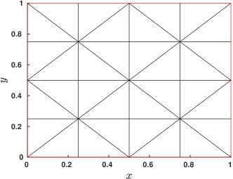
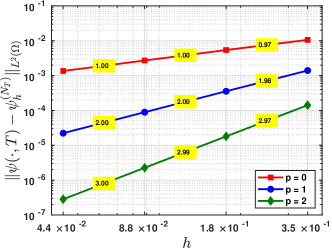
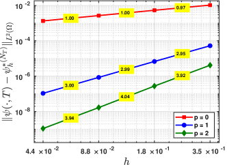
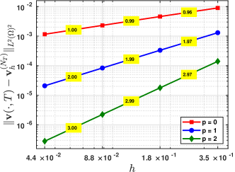
Figure 2: First panel: Example of the simplicial meshes used in the numerical examples. Remaining panels: $h$-convergence of the errors in (6.4) at the final time $T=1$s for the test case with exact solution (6.3). The numbers in the yellow rectangles denote the experimental rates of convergence.

6.3 $\delta$-convergence

We now validate the convergence of the method when the sound diffusivity parameter $\delta$ tends to zero. To do so, we consider the Westervelt equation in (1.1) on the domain $Q_{T}=(0,1)^{2}\times(0,T)$, with parameters $c=1\text{m}\text{s}^{-1}$ and $k=0.3\text{s}^{2}\text{m}^{-2}$. The initial data are given by

$$\psi_{0}(x,y)=10^{-2}\sin(\pi x)\sin(\pi y),\qquad\psi_{1}(x,y)=\sin(\pi x)\sin(\pi y),$$ (6.5)

the spatial mesh is taken as in Figure 2(left panel in the first row), and the parameters $(\gamma,\beta)$ and the time step is chosen as in the previous experiment; cf. [14, §2.4.2]. We consider piecewise constant $(p=0)$ and piecewise linear $(p=1)$ approximations, and $\delta=10^{-2i}$ with $i=1,\ldots,5$.

In Figure 3, we show in log-log scale the following errors computed at the final time $T=1$s

$$\|\psi_{h}^{(\delta)}-\psi_{h}^{(0)}\|_{L^{2}(\Omega)}\quad\text{ and }\quad\|\underaccent{\bar}{\boldsymbol{v}}_{h}^{(\delta)}-\underaccent{\bar}{\boldsymbol{v}}_{h}^{(0)}\|_{L^{2}(\Omega)^{2}}.$$ (6.6)

Convergence rates of order $\mathcal{O}(\delta)$ are observed for both errors. For $p=1$, these results are in agreement with estimate (5.2b), and suggest that estimate (5.2a) may be not sharp. In fact, in [14, Thm. 2.2], convergence rates of order $\mathcal{O}(\delta)$ were established for the standard finite element method by exploiting the relation $\underaccent{\bar}{\boldsymbol{v}}_{h}=\nabla\psi_{h}$. Moreover, it is likely that the exact solution is more regular than assumed in Theorem 4.1, in which case one could show full convergence rates of order $\mathcal{O}(\delta)$ in (5.2a), by deriving higher-order energy stability estimates.

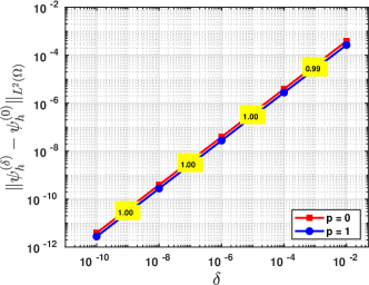
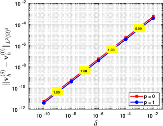
Figure 3: $\delta$-convergence of the errors in (6.6) at the final time $T=1$s for the test case in Section 6.3.

6.4 Steepening of a wavefront

In this experiment, we illustrate the effect of the nonlinearity parameter $k$ on the solution. We consider the Westervelt equation in (1.1) on the domain $Q_{T}=(0,1)^{2}\times(0,T)$, with parameters $c=1500\text{m}\text{s}^{-1}$, $\delta=6\times 10^{-9}\text{m}\text{s}^{-1}$, and $k=-10\text{s}^{2}\text{m}^{-2}$. We consider homogeneous initial conditions and the following forcing term

$$\varphi(x,y,t)=\frac{a}{\sqrt{\sigma}}\exp(-\alpha t)\exp\Big{(}-\frac{(x-0.5)^{2}+(y-0.5)^{2}}{2\sigma^{2}}\Big{)},$$ (6.7)

where $a=400$, $\alpha=5\times 10^{4}$, and $\sigma=3\times 10^{-2}$; cf. [29, §6].

We employ a simplicial mesh $\mathcal{T}_{h}$ with $h\approx 8.83\times 10^{-2}$, a fixed time step $\Delta t=10^{-6}$, and $p=5$. In order to deal with the steepening of the wave, the parameters for the Newmark scheme are chosen as $(\gamma,\beta)=(0.85,0.45)$. In Figure 4(left panels), we show the approximation of $\partial_{t}\psi$ obtained at $t=5\times 10^{-5}$s and $t=2\times 10^{-4}$s. In Figure 4(right panels), we compare the approximation of $\partial_{t}{\psi}$ obtained for the nonlinear Westervelt equation ($k=-10$) and the damped linear wave equation ($k=0$) along the line $y=0.5$. A steepening at the wavefront of the solution is clearly observed for the nonlinear model.

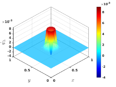
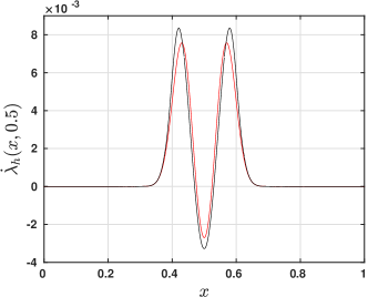
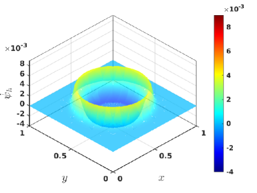
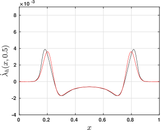
Figure 4: Results obtained at $t=5\times 10^{-5}$s (first row) and $t=2\times 10^{-4}$s (second row) for the test case in Section 6.4. Left panels: Approximation of $\partial_{t}\psi$ obtained for $p=5$ and $k=-10\text{s}^{2}\text{m}^{-2}$. Right panels: Comparison of the approximations obtained for the Westervelt equation (black lines) and the linear damped wave equation (red lines) along the line $y=0.5$.

Since the forcing term $\varphi$ in (6.7) is independent of $\delta$, the $\delta$-convergence estimates in Theorem 5.1 are still valid. In Figure 5, we show the errors in (6.6) obtained at $t=10^{-4}$s. Convergence rates of order $\mathcal{O}(\delta)$ are observed as in the numerical experiment of Section 6.3.

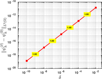
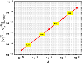
Figure 5: $\delta$-convergence of the errors in (6.6) at $t=10^{-4}$s for the test case in Section 6.4 with degree of approximation $p=5$.

7 Conclusions

In this work, we have designed an asymptotic-preserving HDG method for the numerical simulation of the quasilinear Westervelt equation. We built up a well-posedness and approximation theory for this method, and illustrated our theoretical results with two-dimensional numerical experiments.

Optimal $h$-convergence rates of order $\mathcal{O}(h^{p+1})$ are proven for the approximation of the acoustic particle velocity $\underaccent{\bar}{\boldsymbol{v}}=\nabla\psi$, thus exceeding the expected convergence rates for most standard DG methods. Moreover, we have proven the convergence of the discrete approximation to the vanishing viscosity limit when the sound diffusivity parameter $\delta$ tends to zero. Such a result guarantees the robustness of the method for small values of $\delta$.

Our analysis imposes a restriction on the degree of approximation of the method, namely $p\geq 1$. However, in the numerical experiments, we have obtained convergence of the method with respect to $h$ and $\delta$ also for $p=0$. This is most likely due to the fact that the numerical experiments were performed for two-dimensional domains. Indeed, the case $p=0$ is critical for dimension $d=2$, as commented in Remark 4.4.

The following are three interesting possible directions for the extension of our analysis:

• In view of the close relation between mixed FEM and HDG methods (see, e.g., [10, 7]), we expect that the present analysis can be extended to a unified framework covering a large class of methods.

• More general polytopic meshes could be considered using the theory of $M$-decompositions [5], or hybrid high-order (HHO) methods [13].

• The extension of the method to more general nonlinear sound propagation models such as the Kuznetzov equation [25].

In addition, the superconvergence of order $\mathcal{O}(h^{p+2})$ for the local postprocessed approximation $\psi_{h}^{*}$ defined in (6.1), and the asymptotic-preserving properties of fully discrete schemes as in [14], with special attention to high-order time stepping schemes, are the subject of ongoing research.

Appendix A Proof of low-order energy stability estimate (3.7a)

The ideas for the proof of the stability estimates are inspired by the $\delta$-robust analysis carried out in [29, §5] for the mixed FEM approximation of the Westervelt equation.

Observe that (3.2a)–(3.2c) imply

$$c^{2}\boldsymbol{m}_{h}\left(\partial_{t}{\underaccent{\bar}{\boldsymbol{v}}}_{h},\underaccent{\bar}{\boldsymbol{r}}_{h}\right)+c^{2}b_{h}\left(\partial_{t}{\psi}_{h},\underaccent{\bar}{\boldsymbol{r}}_{h}\right)+c^{2}e_{h}\left(\partial_{t}{\lambda}_{h},\underaccent{\bar}{\boldsymbol{r}}_{h}\right) ={c^{2}}(\partial_{t}\underaccent{\bar}{\boldsymbol{\Upsilon}},\underaccent{\bar}{\boldsymbol{r}}_{h})_{0,\Omega} \forall\underaccent{\bar}{\boldsymbol{r}}_{h}\in\boldsymbol{\mathcal{Q}}_{h}^{p},$$ (A.1a)

$$m_{h}((1+2k\alpha_{h})\partial_{tt}{\psi}_{h},w_{h})-c^{2}b_{h}(w_{h},\widetilde{\underaccent{\bar}{\boldsymbol{v}}}_{h})$$

$$+c^{2}s_{h}(\widetilde{\psi}_{h},w_{h})+c^{2}f_{h}(\widetilde{\lambda}_{h},w_{h}) =(\varphi,w_{h})_{0,\Omega} \forall w_{h}\in\mathcal{S}_{h}^{p},$$ (A.1b)

$$-c^{2}e_{h}(\mu_{h},\widetilde{\underaccent{\bar}{\boldsymbol{v}}}_{h})+c^{2}f_{h}(\mu_{h},\widetilde{\psi}_{h})+c^{2}g_{h}(\widetilde{\lambda}_{h},\mu_{h}) =0 \forall\mu_{h}\in\mathcal{M}_{h}^{p}.$$ (A.1c)

By taking $\underaccent{\bar}{\boldsymbol{r}}_{h}=\widetilde{\underaccent{\bar}{\boldsymbol{v}}}_{h}$, $w_{h}=\partial_{t}{\psi}_{h}$, and $\mu_{h}=\partial_{t}{\lambda}_{h}$ in (A.1), and summing the results, we get

$$\begin{split}m_{h}((1&+2k\alpha_{h})\partial_{tt}{\psi}_{h},\partial_{t}{\psi}_{h})\\ &+c^{2}\big{(}\boldsymbol{m}_{h}(\partial_{t}{\underaccent{\bar}{\boldsymbol{v}}}_{h},\underaccent{\bar}{\boldsymbol{v}}_{h})+s_{h}(\psi_{h},\partial_{t}{\psi}_{h})+f_{h}(\lambda_{h},\partial_{t}{\psi}_{h})+f_{h}(\partial_{t}{\lambda}_{h},\psi_{h})+g_{h}(\lambda_{h},\partial_{t}{\lambda}_{h})\big{)}\\ &+\delta\left(\boldsymbol{m}_{h}(\partial_{t}{\underaccent{\bar}{\boldsymbol{v}}}_{h},\partial_{t}{\underaccent{\bar}{\boldsymbol{v}}}_{h})+s_{h}(\partial_{t}{\psi}_{h},\partial_{t}{\psi}_{h})+2f_{h}(\partial_{t}{\lambda}_{h},\partial_{t}{\psi}_{h})+g_{h}(\partial_{t}{\lambda}_{h},\partial_{t}{\lambda}_{h})\right)\\ &\quad=c^{2}(\partial_{t}\underaccent{\bar}{\boldsymbol{\Upsilon}},\underaccent{\bar}{\boldsymbol{v}}_{h})_{0,\Omega}+\delta(\partial_{t}\underaccent{\bar}{\boldsymbol{\Upsilon}},\partial_{t}{\underaccent{\bar}{\boldsymbol{v}}}_{h})_{0,\Omega}+(\varphi,\partial_{t}{\psi}_{h})_{0,\Omega}.\end{split}$$ (A.2)

Moreover, the following identities follow from the definition of the discrete bilinear forms $m_{h}(\cdot,\cdot)$, $s_{h}(\cdot,\cdot)$, $f_{h}(\cdot,\cdot)$, and $g_{h}(\cdot,\cdot)$:

$$m_{h}((1+2k\alpha_{h})\partial_{tt}{\psi}_{h},\partial_{t}{\psi}_{h})=\frac{1}{2}\frac{d}{dt}\|\sqrt{1+{2}k\alpha_{h}(\cdot,t)}\partial_{t}{\psi}_{h}\|_{L^{2}(\Omega)}^{2}-m_{h}(k\partial_{t}{\alpha}_{h}\partial_{t}{\psi}_{h},\partial_{t}{\psi}_{h}),$$ (A.3a)

$$\boldsymbol{m}_{h}(\partial_{t}{\underaccent{\bar}{\boldsymbol{v}}}_{h},\underaccent{\bar}{\boldsymbol{v}}_{h})+s_{h}(\psi_{h},\partial_{t}{\psi}_{h})+f_{h}(\lambda_{h},\partial_{t}{\psi}_{h})+f_{h}(\partial_{t}{\lambda}_{h},\psi_{h})+g_{h}(\lambda_{h},\partial_{t}{\lambda}_{h})$$

$$\qquad\qquad=\frac{1}{2}\frac{d}{dt}\left(\|\underaccent{\bar}{\boldsymbol{v}}_{h}\|_{L^{2}(\Omega)^{d}}^{2}+\|\tau^{\frac{1}{2}}(\lambda_{h}-\psi_{h})\|_{L^{2}((\partial\mathcal{T}_{h})^{\circ})}^{2}+\|\tau^{\frac{1}{2}}{\partial_{t}{\psi}_{h}}\|_{L^{2}((\partial\mathcal{T}_{h})^{\mathcal{D}})}^{2}\right),$$ (A.3b)

$$\boldsymbol{m}_{h}(\partial_{t}{\underaccent{\bar}{\boldsymbol{v}}}_{h},\partial_{t}{\underaccent{\bar}{\boldsymbol{v}}}_{h})+s_{h}(\partial_{t}{\psi}_{h},\partial_{t}{\psi}_{h})+2f_{h}(\partial_{t}{\lambda}_{h},\partial_{t}{\psi}_{h})+g_{h}(\partial_{t}{\lambda}_{h},\partial_{t}{\lambda}_{h})$$

$$\qquad\qquad=\|\partial_{t}{\underaccent{\bar}{\boldsymbol{v}}}_{h}\|_{L^{2}(\Omega)^{d}}^{2}+\|\tau^{\frac{1}{2}}(\partial_{t}{\lambda}_{h}-\partial_{t}{\psi}_{h})\|_{L^{2}((\partial\mathcal{T}_{h})^{\circ})}^{2}+\|\tau^{\frac{1}{2}}\partial_{t}{\psi}_{h}\|_{L^{2}((\partial\mathcal{T}_{h})^{\mathcal{D}})}^{2}.$$ (A.3c)

Substituting the identities (A.3a)–(A.3c) into (A.2), we get

$$\frac{d}{dt}\mathcal{E}_{h}^{(0)}[\psi_{h},\underaccent{\bar}{\boldsymbol{v}}_{h},\lambda_{h}](t) +\delta\left(\|\partial_{t}{\underaccent{\bar}{\boldsymbol{v}}}_{h}\|_{L^{2}(\Omega)^{d}}^{2}+\|\tau^{\frac{1}{2}}(\partial_{t}{\lambda}_{h}-\partial_{t}{\psi}_{h})\|_{L^{2}((\partial\mathcal{T}_{h})^{\circ})}^{2}+\|\tau^{\frac{1}{2}}\partial_{t}{\lambda}_{h}\|_{L^{2}((\partial\mathcal{T}_{h})^{\mathcal{D}})}^{2}\right)$$

$$= \int_{\Omega}k\partial_{t}{\alpha}_{h}{(\partial_{t}{\psi}_{h})^{2}}\text{d}\boldsymbol{x}+c^{2}(\partial_{t}\underaccent{\bar}{\boldsymbol{\Upsilon}},\underaccent{\bar}{\boldsymbol{v}}_{h})_{0,\Omega}+\delta(\partial_{t}\underaccent{\bar}{\boldsymbol{\Upsilon}},\partial_{t}{\underaccent{\bar}{\boldsymbol{v}}}_{h})_{0,\Omega}+(\varphi,\partial_{t}{\psi}_{h})_{0,\Omega}.$$ (A.4)

All the terms multiplied by ${\delta}$ on the left-hand side of (A.4) are nonnegative. By using the Cauchy–Schwarz and the Young inequalities, we get

$$\delta(\partial_{t}\underaccent{\bar}{\boldsymbol{\Upsilon}},\partial_{t}{\underaccent{\bar}{\boldsymbol{v}}}_{h})_{0,\Omega}\leq\frac{\delta}{4}\|\partial_{t}\underaccent{\bar}{\boldsymbol{\Upsilon}}\|_{L^{2}(\Omega)^{d}}^{2}+\delta\|\partial_{t}{\underaccent{\bar}{\boldsymbol{v}}}_{h}\|_{L^{2}(\Omega)^{d}}^{2},$$

so the second term cancels out with the one on the left-hand side of (A.4). Integrating identity (A.4) over $(0,t)$ and using the Hölder and Young inequalities, we deduce that

$$\begin{split}\mathcal{E}_{h}^{(0)}[\psi_{h},\underaccent{\bar}{\boldsymbol{v}}_{h},\lambda_{h}](t)\leq&\ \mathcal{E}_{h}^{(0)}[\psi_{h},\underaccent{\bar}{\boldsymbol{v}}_{h},\lambda_{h}](0)\\ &+\left(\|k{(1+2k\alpha_{h})^{-1}}\partial_{t}{\alpha}_{h}\|_{L^{1}(0,t;L^{\infty}(\Omega))}+\frac{\gamma}{2}\right)\|\sqrt{1+{2}k\alpha_{h}}\partial_{t}{\psi}_{h}\|_{L^{\infty}(0,t;L^{2}(\Omega))}^{2}\\ &+\frac{1}{2\gamma}\|(1+{2}k\alpha_{h})^{-\frac{1}{2}}\varphi\|_{L^{1}(0,t;L^{2}(\Omega))}^{2}+{\frac{\delta}{4}}\|\partial_{t}\underaccent{\bar}{\boldsymbol{\Upsilon}}\|_{L^{2}(0,t;L^{2}(\Omega)^{d})}^{2}\\ &+{\frac{c^{2}}{2{\sigma_{0}}}}\|\partial_{t}\underaccent{\bar}{\boldsymbol{\Upsilon}}\|_{L^{1}(0,t;L^{2}(\Omega)^{d})}^{2}+{\frac{c^{2}{\sigma_{0}}}{2}}\|{\underaccent{\bar}{\boldsymbol{v}}_{h}}\|_{L^{\infty}(0,t;L^{2}(\Omega)^{d})}^{2},\end{split}$$ (A.5)

for all $\gamma>0$.

Moreover, by using the Hölder inequality, we have the following bounds

$$\begin{split}\|(1+2k\alpha_{h})^{-\frac{1}{2}}\varphi\|_{L^{1}(0,t;L^{2}(\Omega))}^{2}&\leq t\|(1+2k\alpha_{h})^{-\frac{1}{2}}\varphi\|_{L^{2}(0,t;L^{2}(\Omega))}^{2},\\ \|\partial_{t}\underaccent{\bar}{\boldsymbol{\Upsilon}}\|_{L^{1}(0,t;L^{2}(\Omega)^{d})}^{2}&\leq t\|\partial_{t}\underaccent{\bar}{\boldsymbol{\Upsilon}}\|_{L^{2}(0,t;L^{2}(\Omega)^{d})}^{2},\\ \|\underaccent{\bar}{\boldsymbol{v}}_{h}\|_{L^{\infty}(0,t;L^{2}(\Omega)^{d})}^{2}&\leq\sup_{s\in(0,t)}\|\underaccent{\bar}{\boldsymbol{v}}_{h}\|_{L^{2}(\Omega)^{d}}^{2}.\end{split}$$ (A.6)

Finally, smallness assumption (3.4) states that there exist constants $0<\gamma_{0}<{\sigma_{0}}<1$ independent of $h$ and ${\delta}$ such that

$$\|k{(1+2k\alpha_{h})^{-1}}\partial_{t}{\alpha}_{h}\|_{L^{1}(0,t;L^{\infty}(\Omega))}+\frac{\gamma_{0}}{2}\leq\frac{|k|}{1-2|k|\underline{\alpha}}\|\partial_{t}{\alpha}_{h}\|_{L^{1}(0,t;L^{\infty}(\Omega))}+\frac{\gamma_{0}}{2}\leq\frac{{\sigma_{0}}}{2},$$

which, together with (A.5) and (A.6), gives the low-order energy estimate in (3.7a).

Appendix B Proof of high-order energy stability estimate (3.7b)

The proof of the high-order stability estimate in (3.7b) follows by considering the time-differentiated system

$$c^{2}\boldsymbol{m}_{h}\left(\partial_{tt}{\underaccent{\bar}{\boldsymbol{v}}}_{h},\underaccent{\bar}{\boldsymbol{r}}_{h}\right)+c^{2}b_{h}\left(\partial_{tt}{\psi}_{h},\underaccent{\bar}{\boldsymbol{r}}_{h}\right)+c^{2}e_{h}\left(\partial_{tt}{\lambda}_{h},\underaccent{\bar}{\boldsymbol{r}}_{h}\right) =(\partial_{tt}\underaccent{\bar}{\boldsymbol{\Upsilon}},\underaccent{\bar}{\boldsymbol{r}}_{h})_{0,\Omega} \forall\underaccent{\bar}{\boldsymbol{r}}_{h}\in\boldsymbol{\mathcal{Q}}_{h}^{p},$$

$$m_{h}((1+2k\alpha_{h})\partial_{ttt}{\psi}_{h},w_{h})+m_{h}(2k\partial_{t}{\alpha}_{h}\partial_{tt}{\psi}_{h},w_{h})-c^{2}b_{h}(w_{h},\partial_{t}{\widetilde{\underaccent{\bar}{\boldsymbol{v}}}}_{h})$$

$$+c^{2}f_{h}(\partial_{t}{\widetilde{\lambda}}_{h},w_{h})+c^{2}s_{h}(\partial_{t}{\widetilde{\psi}}_{h},w_{h}) =(\partial_{t}{\varphi},w_{h})_{0,\Omega} \forall w_{h}\in\mathcal{S}_{h}^{p},$$

$$-c^{2}e_{h}(\mu_{h},\partial_{t}{\widetilde{\underaccent{\bar}{\boldsymbol{v}}}}_{h})+c^{2}f_{h}(\mu_{h},\partial_{t}{\widetilde{\psi}}_{h})+c^{2}g_{h}(\partial_{t}{\widetilde{\lambda}}_{h},\mu_{h}) =0 \forall\mu_{h}\in\mathcal{M}_{h}^{p},$$

choosing $\underaccent{\bar}{\boldsymbol{r}}_{h}=\partial_{t}{\widetilde{\underaccent{\bar}{\boldsymbol{v}}}}_{h}$, $w_{h}=\partial_{tt}{\psi}_{h}$, and $\mu_{h}=\partial_{tt}{\lambda}_{h}$ as test functions, and summing the resulting equations. The remaining steps are similar to those exposed in Appendix A for the low-order estimate in (3.7a), and are therefore omitted.

References

- [1] R. P. Agarwal, M. Meehan, and D. O’regan. Fixed Point Theory and Applications, volume 141. Cambridge University Press, 2001.
- [2] P.-F. Antonietti, I. Mazzieri, M. Muhr, V. Nikolić, and B. Wohlmuth. A high-order discontinuous Galerkin method for nonlinear sound waves. J. Comput. Phys., 415:109484, 27, 2020.
- [3] S. C. Brenner and L. R. Scott. The mathematical theory of finite element methods, volume 15 of Texts in Applied Mathematics. Springer, New York, third edition, 2008.
- [4] B. Cockburn, B. Dong, and J. Guzmán. A superconvergent LDG-hybridizable Galerkin method for second-order elliptic problems. Math. Comp., 77(264):1887–1916, 2008.
- [5] B. Cockburn, G. Fu, and F.-J. Sayas. Superconvergence by -decompositions. Part I: General theory for HDG methods for diffusion. Math. Comp., 86(306):1609–1641, 2017.
- [6] B. Cockburn, Z. Fu, A. Hungria, L. Ji, M.-A. Sánchez, and F.-J. Sayas. Stormer-Numerov HDG methods for acoustic waves. J. Sci. Comput., 75(2):597–624, 2018.
- [7] B. Cockburn, J. Gopalakrishnan, and R. Lazarov. Unified hybridization of discontinuous Galerkin, mixed, and continuous Galerkin methods for second order elliptic problems. SIAM J. Numer. Anal., 47(2):1319–1365, 2009.
- [8] B. Cockburn, J. Gopalakrishnan, and F.-J. Sayas. A projection-based error analysis of HDG methods. Math. Comp., 79(271):1351–1367, 2010.
- [9] B. Cockburn, J. Guzmán, and H. Wang. Superconvergent discontinuous Galerkin methods for second-order elliptic problems. Math. Comp., 78(265):1–24, 2009.
- [10] B. Cockburn, W. Qiu, and K. Shi. Conditions for superconvergence of HDG methods for second-order elliptic problems. Math. Comp., 81(279):1327–1353, 2012.
- [11] B. Cockburn and V. Quenneville-Bélair. Uniform-in-time superconvergence of the HDG methods for the acoustic wave equation. Math. Comp., 83(285):65–85, 2014.
- [12] L. Demi and M. D. Verweij. Nonlinear Acoustics. In Comprehensive Biomedical Physics, pages 387–399. Elsevier, Oxford, 2014.
- [13] D. A. Di Pietro, A. Ern, and S. Lemaire. An arbitrary-order and compact-stencil discretization of diffusion on general meshes based on local reconstruction operators. Comput. Methods Appl. Math., 14(4):461–472, 2014.
- [14] B. Dörich and V. Nikolić. Robust fully discrete error bounds for the Kuznetsov equation in the inviscid limit. arXiv:2401.06492, 2024.
- [15] R. Griesmaier and P. Monk. Discretization of the wave equation using continuous elements in time and a hybridizable discontinuous Galerkin method in space. J. Sci. Comput., 58(2):472–498, 2014.
- [16] M. Hochbruck and B. Maier. Error analysis for space discretizations of quasilinear wave-type equations. IMA J. Numer. Anal., 42(3):1963–1990, 2022.
- [17] T. J. R. Hughes. The finite element method. Prentice Hall, Inc., Englewood Cliffs, NJ, 1987.
- [18] B. Kaltenbacher and I. Lasiecka. Global existence and exponential decay rates for the Westervelt equation. Discrete Contin. Dyn. Syst. Ser. S, 2(3):503–523, 2009.
- [19] B. Kaltenbacher, M. Meliani, and V. Nikolić. Limiting behavior of quasilinear wave equations with fractional-type dissipation. Adv. Nonlinear Stud. To appear, 2024.
- [20] B. Kaltenbacher and V. Nikolić. Parabolic approximation of quasilinear wave equations with applications in nonlinear acoustics. SIAM J. Math. Anal., 54(2):1593–1622, 2022.
- [21] B. Kaltenbacher and G. Peichl. The shape derivative for an optimization problem in lithotripsy. Evol. Equ. Control Theory, 5(3):399–429, 2016.
- [22] M. Kaltenbacher. Numerical Simulation of Mechatronic Sensors and Actuators, volume 2. Springer, 2007.
- [23] M. Kaltenbacher, H. Landes, J. Hoffelner, and R Simkovics. Use of modern simulation for industrial applications of high power ultrasonics. In 2002 IEEE Ultrasonics Symposium, volume 1, pages 673–678. IEEE, 2002.
- [24] S. Kawashima and Y. Shibata. Global existence and exponential stability of small solutions to nonlinear viscoelasticity. Comm. Math. Phys., 148(1):189–208, 1992.
- [25] V. P. Kuznetsov. Equations of nonlinear acoustics. Soviet Physics: Acoustic, 16:467–470, 1970.
- [26] B. Maier. Error analysis for space and time discretizations of quasilinear wave-type equations. PhD thesis, Karlsruher Institut für Technologie (KIT), 2020.
- [27] M. Meliani. A unified analysis framework for generalized fractional Moore-Gibson-Thompson equations: well-posedness and singular limits. Fract. Calc. Appl. Anal., 26(6):2540–2579, 2023.
- [28] M. Meliani and V. Nikolić. Analysis of general shape optimization problems in nonlinear acoustics. Appl. Math. Optim., 86(3):Paper No. 39, 35, 2022.
- [29] M. Meliani and V. Nikolić. Mixed approximation of nonlinear acoustic equations: Well-posedness and a priori error analysis. Appl. Numer. Math., 198:94–111, 2024.
- [30] S. Meyer and M. Wilke. Optimal regularity and long-time behavior of solutions for the Westervelt equation. Appl. Math. Optim., 64(2):257–271, 2011.
- [31] N. C. Nguyen, J. Peraire, and B. Cockburn. Hybridizable discontinuous Galerkin methods for the time-harmonic Maxwell’s equations. J. Comput. Phys., 230(19):7151–7175, 2011.
- [32] V. Nikolić. Asymptotic-preserving finite element analysis of Westervelt-type wave equations. arXiv:2303.10743, 2023.
- [33] V. Nikolić and B. Wohlmuth. A priori error estimates for the finite element approximation of Westervelt’s quasi-linear acoustic wave equation. SIAM J. Numer. Anal., 57(4):1897–1918, 2019.
- [34] M. A. Sánchez, C. Ciuca, N. C. Nguyen, J. Peraire, and B. Cockburn. Symplectic Hamiltonian HDG methods for wave propagation phenomena. J. Comput. Phys., 350:951–973, 2017.
- [35] I. Shevchenko and B. Kaltenbacher. Absorbing boundary conditions for nonlinear acoustics: the Westervelt equation. J. Comput. Phys., 302:200–221, 2015.
- [36] P. J. Westervelt. Parametric acoustic array. The Journal of the Acoustical Society of America, 35(4):535–537, 1963.