Optimisation challenge for superconducting adiabatic neural network implementing XOR and OR boolean functions

Abstract

In this article, we consider designs of simple analog artificial neural networks based on adiabatic Josephson cells with a sigmoid activation function. A new approach based on the gradient descent method is developed to adjust the circuit parameters, allowing efficient signal transmission between the network layers. The proposed solution is demonstrated on the example of the system implementing XOR and OR logical operations.

I Introduction

A distinctive feature of the current era of information technology evolution is the widespread development and implementation of artificial intelligence (AI) Zbontar and LeCun (2016); Tolosana et al. (2018); Kaya and Bilge (2019); Ruiz et al. (2020); Wang and Deng (2021); Ilina et al. (2022). In order to effectively solve a number of tasks, specialised hardware implementation of AI systems is required Le Gallo et al. (2023); Modha et al. (2023). The most popular and exciting at the moment are the so-called neuromorphic chips or neuromorphic processors. In this field, world giants such as Intel (Loihi 1 and Loihi 2) and IBM (TrueNorth, NorthPole) have made their mark. In addition to neuromorphic processors, there are machine learning processors (Intel Movidius Myriad 2, Mobileye EyeQ) designed to accelerate data processing (video, machine vision, etc.) and tensor processors (Google TPU, Huawei Ascend, Intel Nervana NNP) designed to accelerate arithmetic operations. While the latter two types have been successfully implemented in modern hardware platforms (smartphones, cloud computing, etc.), neuromorphic processors, despite their potential, are unfortunately not yet widespread and remain mostly at the laboratory production and testing stage Kumar (2013); Prezioso et al. (2015); Bose et al. (2017); Davies et al. (2018); Cheng et al. (2018); Jeong and Shi (2018); DeBole et al. (2019); Arute et al. (2019); Berggren et al. (2020); Wan et al. (2022).

There are a number of post-Moore technology platforms that enable the realisation of AI technologies at the hardware level, promising advances in performance and/or energy efficiency. Optical neuromorphic networks are an excellent example Feldmann et al. (2019); Jha et al. (2022) of energy-efficient systems with high performance. Photonic-superconducting interfaces Singh and Zheludev (2014); Fan et al. (2018); Gu et al. (2017); Berman et al. (2006) and other hybrid optical-superconducting neural networks Shainline et al. (2017, 2018, 2019); Schneider et al. (2022) were once a major milestone in the development of this field of applied science. These systems used light pulses to transmit signals and superconducting circuits based on quantum interferometers to process and store information. Superconducting elements are known for their high energy efficiency Crotty et al. (2010); Russek et al. (2016); Schneider et al. (2018); Toomey et al. (2020); Ishida et al. (2021); Zhang et al. (2021); Semenov et al. (2021); Casaburi and Hadfield (2022); Feldhoff and Toepfer (2024). In the context of modern data centres that require massive cooling, superconductor-based hybrid computers may become quite competitive players. It is also worth noting that quantum computers Siddiqi (2021); Vozhakov et al. (2022); Calzona and Carrega (2022) are now being developed on the basis of superconductor technology. Therefore, the creation of superconducting neuromorphic chips capable of hybridisation with quantum computers (QCs) seems very reasonable. An example might be qubit spectrum detection of a QC’s output signal, or a QC’s calculation of synaptic weights for an externally tunable artificial neural network. This study focuses on the optimisation of superconducting basic elements and their interconnections specified for superconducting logic gates in neuromorphic systems (Figure 1).

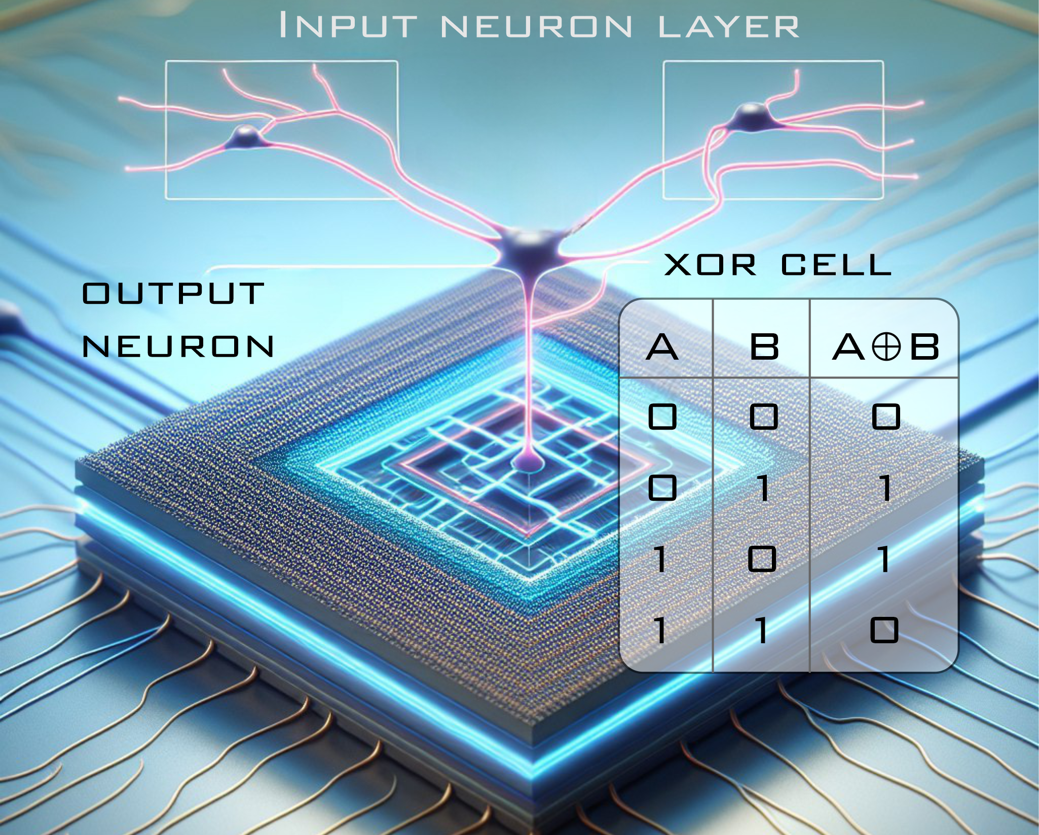
Figure 1: OpenAI’s DALLE 3 prompt-generated image of a superconducting neural network simulating an XOR operation.

It is also necessary to mention here imitations of neural activity of living tissues with the help of superconducting electronics using Josephson contacts Crotty et al. (2010); Russek et al. (2016); Segall et al. (2017); Schneider et al. (2018); Toomey et al. (2020); Zhang et al. (2021); Feldhoff and Toepfer (2021); Goteti and Dynes (2021); Chalkiadakis and Hizanidis (2022); Schneider et al. (2022); Schegolev et al. (2023); Crotty et al. (2023); Feldhoff and Toepfer (2024). These works demonstrate the operation of bio-inspired neurons (capable of reproducing basic biological patterns of nervous activity, such as excitability, spiking and bursting) and synapses, as well as simple neural networks. The possibility of using Josephson circuits for modeling and simulating the work of neurons and tissues, as well as for more applied tasks (e.g., recognition), will allow reaching a new level of performance (computational and modeling speed, energy efficiency) of spiking neural networks.

Previously, we presented the concept of an adiabatic interferometer-based superconducting neuron Schegolev et al. (2020); Bastrakova et al. (2021); Ionin et al. (2023a), capable of operating in classical and quantum modes with ultra-low energy dissipation per operation (in the zJ range) Takeuchi et al. (2020); Khazali and Mølmer (2020); Ayala et al. (2020); Yamazaki et al. (2021); Setiawan et al. (2021); Bastrakova et al. (2022); Pashin et al. (2023); Mizushima et al. (2023). The development of an adiabatic perceptron requires the realisation of a large number of connections between neurons via superconducting synapses Schegolev et al. (2020). Good synapses for perceptron-type networks should have the following important properties: a wide range of weights (both negative and positive, as well as zero), low noise, signal type preservation (high linearity), and circuit simplicity (as few components as possible). Based on these requirements we used the synapse scheme first presented in Bakurskiy et al. (2020).

Combining these elements into an analog network implies the generally difficult task of studying the complex nonlinear dynamics of the system. We propose a solution to this problem and demonstrate the results on the example of a three-neuron network simulating an XOR and OR logic gates.

II The model for two coupled adiabatic neurons

Before the simulation of the superconducting logic element, we have considered the system of two coupled $S_{c}$-neurons having sigmoid activation function. These basic elements are the superconducting interferometers connected by the inductive synapse, see Figure 2. The formation of the activation functions (flux-to-flux transformations) on individual $S_{c}$-neurons has been previously studied in detail both in classical Schegolev et al. (2020); Bastrakova et al. (2021); Ionin et al. (2023a) and quantum modes Bastrakova et al. (2022); Pashin et al. (2023). Here we consider the interaction between different parts of the system. We choose an inductive synapse instead of the Josephson one Njitacke et al. (2022) because of its absolute linearity of the transfer characteristic and a wide dynamic range Bakurskiy et al. (2020); Schegolev et al. (2022).

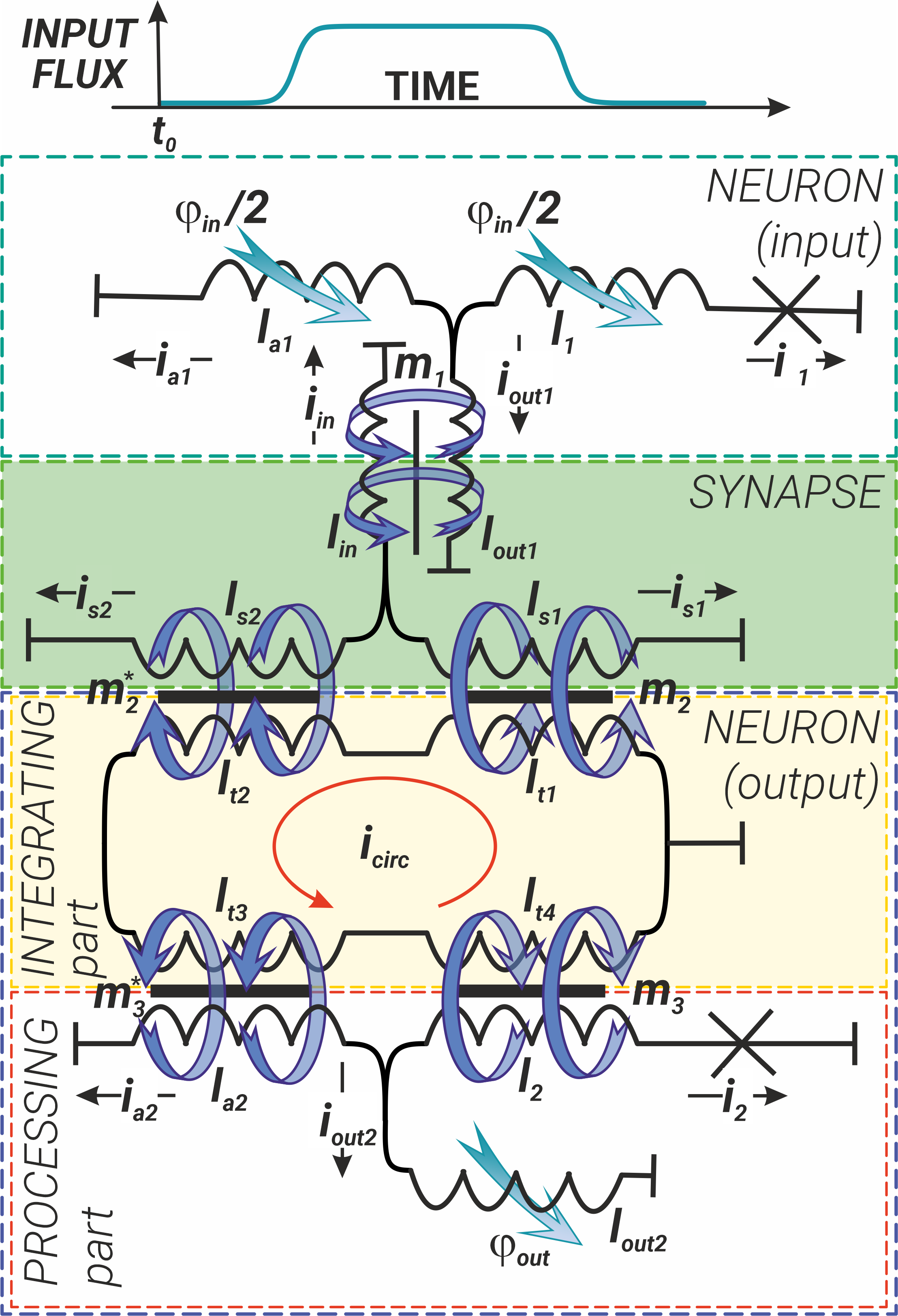
Figure 2: Schematic representation of two coupled $S_{c}$-neurons (input – in cyan box and output – in navy blue box), connected through the inductive synapse (in the green box) and the coupler – integrating part of the output neuron (in the light yellow box). Processing part of the

output neuron is highlighted by red box. Black or red arrows and blue curled arrows indicate currents and corresponding magnetic fluxes, respectively.

The $S_{c}$ neurons (areas outlined by the cyan and navy blue dashed lines in Figure 2) are designed according to the integrating-and-processing principle: the integrating part (IP) collects or $integrates$ all input signals, while the processing part (PP) processes this input signal and generates an output signal. Generally $S_{c}$-neuron consists of three branches (its processing part): two of them (the branches with the inductance $l_{out1,2}$ and the branch with the Josephson junction and the inductance $l_{1,2}$) form the circuit of the so-called quantron. The third branch with a single inductance $l_{a1,2}$ shunts the quantron circuit. In the Figure 2 the IP of the output neuron is highlighted by light yellow box and is formed by a so-called coupler – an inductive ring ($l_{t1,2,3,4}$) that collect output flux from input neuron(s) (the IP of the input neuron is not shown in the Figure 2). The signal in the form of magnetic flux flows from the neuron’s IP to the neuron’s PP through the inductances $l_{1,2}$ and $l_{a1,2}$. The inductance $l_{out1,2}$ is used to transmit the magnetic flux from the $S_{c}$-neuron to subsequent element (in our case the input neuron transmits its signal to the inductive synapse).

The inductive synapse (green box in Figure 2) in turn also has three branches: the input branch (containing the inductance $l_{in}$) is responsible for signal reception, and the branches containing the tunable kinetic inductances $l_{s1}$ and $l_{s2}$ Annunziata et al. (2010); Splitthoff et al. (2022); Klenov et al. (2019); Bakurskiy et al. (2020) provide its further transmission. Synapse adjustment is realised by external magnetic or spin-current influence (not shown in Figure 2). By changing the values of the inductances $l_{s1}$ and $l_{s2}$ one can vary the weight of the synapse.

In the following, all inductances are normalised to the characteristic Josephson inductance of the output neuron Josephson junction, $\Phi_{0}/2\pi I_{C_{2}}$, where $I_{C_{2}}$ is the critical current of this junction. Magnetic fluxes are normalised to the magnetic flux quantum, $\varphi=2\pi\Phi/\Phi_{0}$, $\Phi_{0}=h/2e$.

The input signal ($\varphi_{in}$) has been set in the form of a smoothed trapezoid, which makes it possible to take into account both the rising (rise time) and falling (fall time) phases of the signal. The duration of the plateau section can also be controlled:

$$\varphi_{in}(t)=A_{in}\cdot\left\{\frac{1}{1+\exp(-2D(t-t_{1}))}+\right.$$ (1)

$$\left.\frac{1}{1+\exp(2D(t-t_{2}))}\right\}-A_{in}.$$

The parameters $A_{in}$ and $D$ set the level and the rise/fall rate of the input magnetic flux respectively. As it is shown in Bastrakova et al. (2021), the input signal in the form of (1) allows to obtain the sigmoid transfer function of the $S_{c}$-neuron for certain values of the inductances.

The circuit shown in Figure 2 is described by the following system of equations:

$$\begin{cases}i_{a1}+i_{1}+i_{out1}=0,\\ \varphi_{1}-\frac{\varphi_{in}}{2}+i_{1}l_{1}=i_{out1}l_{out1}+m_{1}i_{in},\\ \varphi_{1}-\frac{\varphi_{in}}{2}+i_{1}l_{1}=i_{a1}l_{a_{1}}+\frac{\varphi_{in}}{2},\\ i_{in}+i_{s1}+i_{s2}=0,\\ i_{s1}(l_{s1}+l_{p})+m_{2}i_{circ}=i_{s2}(l_{s2}+l_{p})-m^{*}_{2}i_{circ},\\ i_{s1}(l_{s1}+l_{p})+m_{2}i_{circ}=-i_{in}(l_{in}+l_{p})+m_{1}i_{out1},\\ i_{circ}\sum_{j=1}^{4}l_{tj}=i_{2}m_{3}-i_{a2}m^{*}_{3}-i_{s1}m_{2}+i_{s2}m^{*}_{2},\\ i_{2}+i_{a2}+i_{out2}=0,\\ \varphi_{2}-m_{3}i_{circ}+i_{2}l_{2}=i_{out2}l_{out2},\\ \varphi_{2}-m_{3}i_{circ}+i_{2}l_{2}=i_{a2}l_{a_{2}}+m^{*}_{3}i_{circ}.\end{cases}$$ (2)

Here $\varphi_{1,2}$ are the superconducting phase drops at the Josephson junctions of the input and output neurons, $l_{p}$ is an additional non-adjustable (parasitic) inductance in this circuit, which is not explicitly shown in the Figure 2, but is taken into account in our calculations. The currents $i_{a1}$, $i_{1}$ and $i_{out1}$ are the currents flowing through the corresponding inductances in the input neuron $l_{a1}$, $l_{1}$ and $l_{out1}$. The currents $i_{in}$, $i_{s1}$ and $i_{s2}$ are the currents in the synapse, flowing through $l_{in}$, $l_{s1}$ and $l_{s2}$. The currents $i_{s1}$ and $i_{s2}$ induce the circulating current $i_{circ}$ in the integrating part of the output neuron. The circulating current in turn induces currents in the processing part of the output neuron $i_{2}$, $i_{s2}$ and $i_{out2}$ which flow through the inductances $l_{a2}$, $l_{2}$ and $l_{out2}$. All currents in (2) are normalised by $I_{C_{2}}$. The parameters $m_{k}$ and $m_{k}^{*}$ are mutual inductance coefficients in transformer elements ($k=1,2,3$), which are considered equal to the average values of the inductances constituting the corresponding transformers.

It can be shown that the currents in the proposed circuit (Figure 2) have a simple relationship with the phases of the Josephson junctions and the external flux:

$$i_{\gamma}=-\kappa_{\gamma}^{(1)}\varphi_{1}-\kappa_{\gamma}^{(2)}\varphi_{2}-\kappa_{\gamma}^{(in)}\varphi_{in}.$$ (3)

Here all coefficients $\kappa_{\gamma}^{(1)}$, $\kappa_{\gamma}^{(2)}$ and $\kappa_{\gamma}^{(in)}$ are obtained from the system of equations (2) and represented in terms of inductances according to Figure 2. The subscript $\gamma=1,2,in,s,a,out$ of the coefficients indicates the current ($i_{1}$, $i_{2}$, $i_{in}$, and $\Delta i_{s}=i_{s1}-i_{s2}$, respectively) to which they belong. The superscript in the formula (3) takes the values of the corresponding phases of the junctions or the input magnetic flux. The analytical expressions for these coefficients are bulky, so they are given in the Supplementary Material.

Note that due to $\varphi_{1}$, $\varphi_{2}$ complex dependence on $\varphi_{in}$, in fact, the currents $i_{\gamma}$ are not linear in any of them. The non-linearity of the system comes from the Josephson junctions, whose currents, $I_{n}$ (where the subscript $n=1,2$ is the index of the junction), can be written as

$$I_{n}=\frac{\hbar}{2e}C_{n}\ddot{\varphi_{n}}+\frac{\hbar}{2eR_{n}}\dot{\varphi_{n}}+I_{C_{n}}\sin\varphi_{n}.$$ (4)

in the frame of the well-known resistively shunted junction model with capacitance (RSJC) Stewart (1968).

Here we consider an energy efficient circuit consisting of tunnel superconducting - insulator - superconducting (SIS) Josephson junctions with a high normal state resistance $R_{n}$, so that the second term in the equation (4) becomes negligibly small and, as modelling shows, does not contribute significantly to the overall dynamics of the system, therefore can be safely omitted.

After normalisation (4) by $I_{C_{2}}$, the equations take the following form:

$$c_{n}\ddot{\varphi_{n}}+i_{C_{n}}\sin\varphi_{n}=i_{n},$$ (5)

where $i_{C_{n}}=I_{C_{n}}/I_{C_{2}}$ is a dimensionless critical current; $t_{C}=\sqrt{\frac{\hbar C_{2}}{2eI_{C_{2}}}}$ is a characteristic time and $\tau=t/t_{C}$ is a dimensionless time; $c_{n}=C_{n}/C_{2}$ is a dimensionless capacity. Note that such systems of interacting neurons can also be considered within the framework of the Hamiltonian formalism. As an example, in the Supplementary Materials, we present the derivation of the Hamiltonian of the system shown in Figure 2. This approach is quite simple and convenient in the case of scaling the circuit to a larger number of layers in a neural network, as well as for numerical modeling of nonlinear dynamics and further study of the quantum mode of operation of the circuit Bastrakova et al. (2022); Pashin et al. (2023), including taking into account the influence of environments.

Solution of the system of equations (5) gives the transfer characteristics of the input and output neurons as a response to the input magnetic flux (1). Previous studies of single $S_{c}$-neurons Bastrakova et al. (2021) have shown that the sigmoid activation function can be realised under the following condition: $l_{n}<\sqrt{l_{outn}^{2}+1}-l_{outn}\equiv l_{n}^{*}$ and $l_{an}=l_{n}+1$. Hence, as in the single-neuron case, we will consider values of inductances $l_{n}<l_{n}^{*}$ at which there are no plasmonic oscillations in the output characteristics of the first (input) and the second (output) neurons.

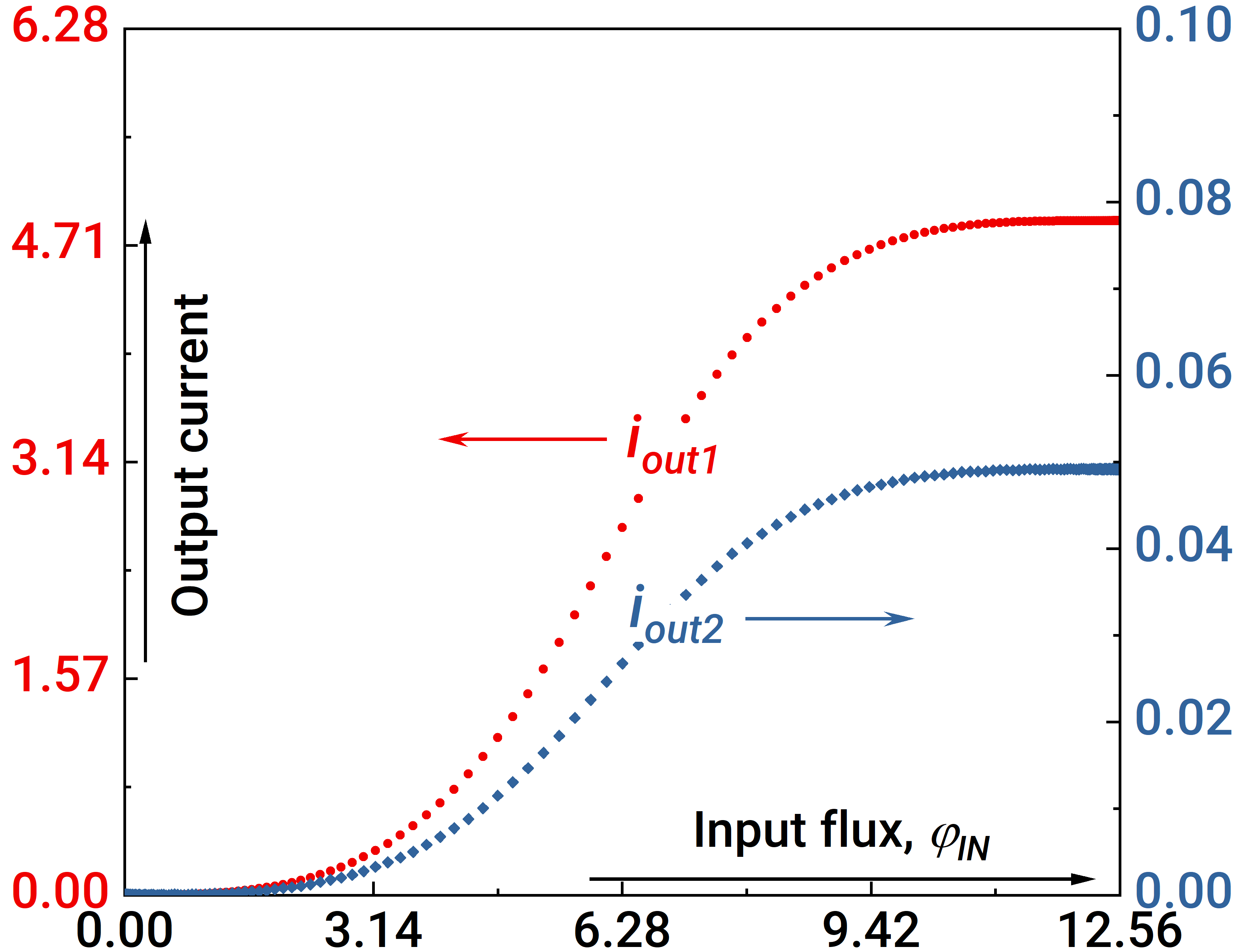
Figure 3: Activation functions for the first (input) and second (output) neurons. The "red" curve corresponds to $i_{out1}$, the "blue" curve corresponds to $i_{out2}$. Parameters of the system: $l_{1,2}=0.2$, $l_{out1}=l_{out2}=1$, $l_{a1,a2}=l_{1,2}+1$, $l_{in}=1$, $l_{t1}=l_{t2}=0.1$, $l_{t3}=l_{t4}=1$, $l_{s1}+l_{s2}=1$, $l_{s1}-l_{s2}=0.9$.

In the first step of the analysis we assume that the coupler inductances should be equal: $l_{t1}=l_{t2}$ and $l_{t3}=l_{t4}$. Figure 3 illustrates the formation of sigmoid activation functions for the input and output neurons under this assumption. It is seen that, the current at the output neuron (blue curve in Figure 3) drops by two orders of magnitude; this drawback reflects the difficulty of practical system implementation. It is also necessary to obtain the synapse weights that are at least in the range from -1 to +1, which turns out to be impossible in some situations (see Figure 4).

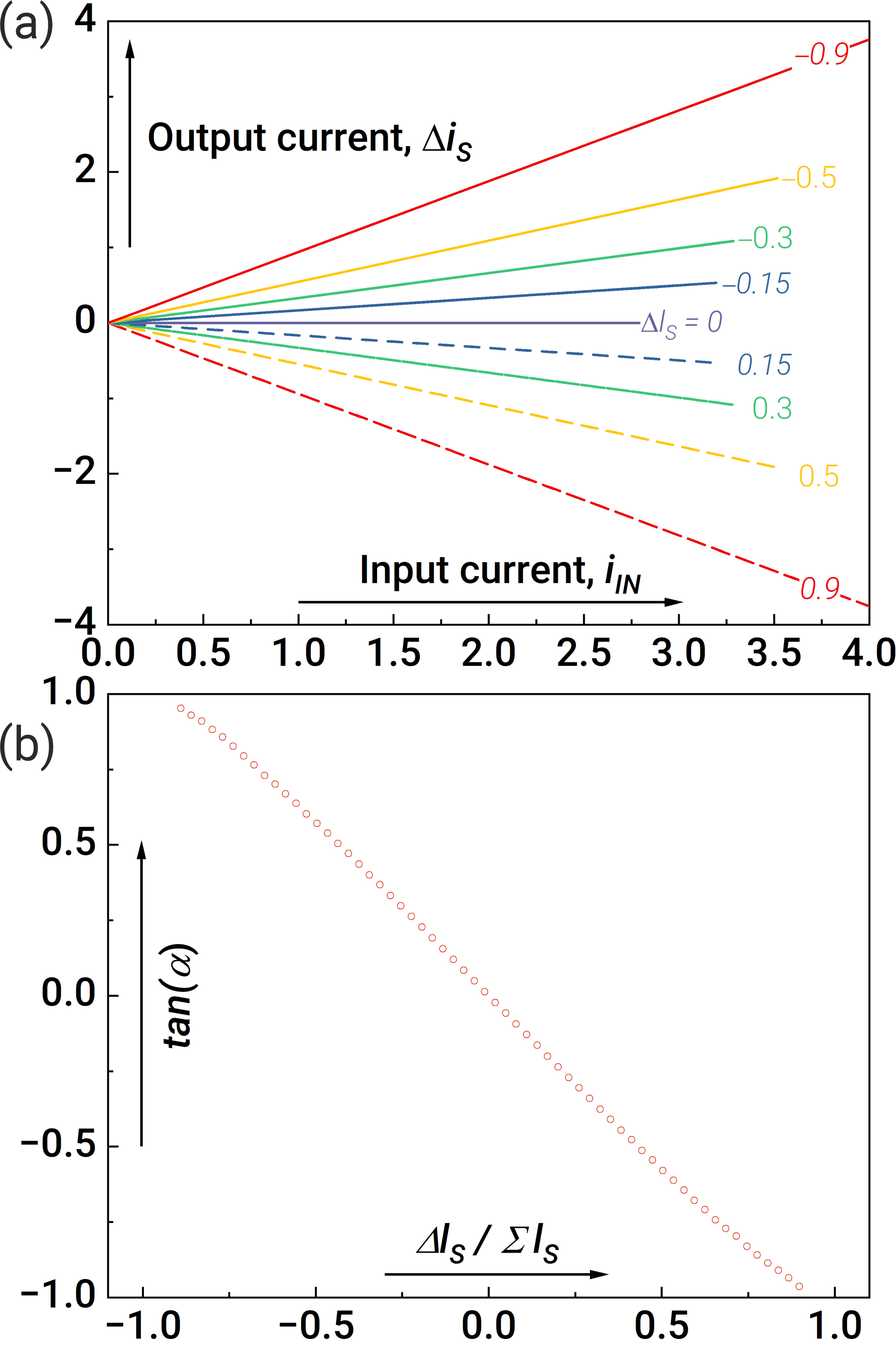
Figure 4: Synaptic weights without system parameters optimisation: (a) dependence of the output current from the synapse ($\Delta i_{s}=i_{s1}-i_{s2}$) as a function of the input current ($i_{in}$) and (b) calculations for the dependence of the slope angle $\alpha$ on $\Delta l_{s}=l_{s1}-l_{s2}$. Parameters of the system: $l_{1,2}=0.2$, $l_{out1}=l_{out2}=1$, $l_{a1,a2}=l_{1,2}+1$, $l_{in}=1$, $l_{t1}=l_{t2}=0.1$, $l_{t3}=l_{t4}=1$, $l_{s1}+l_{s2}=1$.

The above issues imply the need for parameter optimisation. In the next part of the paper, we propose this procedure, which can be generalised to the case of large computing systems.

III Formulation and solution of the optimisation problem

We consider the optimisation problem of a system of two coupled neurons from the point of view of solving the two problems of synapse weights and neuron response magnitudes mentioned above. However, a closer look at these problems reveals that they are closely related: achieving higher values of weights can potentially increase the response magnitude of the output. Therefore, further actions will be aimed at finding a functional describing the synapse weight as a function of the system parameters and finding its extrema using the gradient descent method. As such a functional, we consider the slope angle of the synapse characteristic $\alpha$, which can be expressed analytically in the following form:

$$\tan{\alpha}=\frac{d\Delta i_{s}}{dt}\Big{/}\frac{di_{in}}{dt}=$$ (6)

$$\frac{\kappa^{(1)}_{s}\dot{\varphi}_{1}+\kappa^{(2)}_{s}\dot{\varphi}_{2}+\kappa^{(in)}_{s}\dot{\varphi}_{in}}{\kappa^{(1)}_{in}\dot{\varphi}_{1}+\kappa^{(2)}_{in}\dot{\varphi}_{2}+\kappa^{(in)}_{in}\dot{\varphi}_{in}},$$

When using the gradient descent method, it is necessary to solve a system of differential equations (5) at each step, which is the main computational complexity due to the large number of varied system parameters. To overcome this difficulty, we propose several simplifications.

Since dynamic processes in the system are associated with changes in the input flux and, moreover, take place exactly at the rise/fall time intervals, and the dependence $\Delta i_{s}(i_{in})$ is linear, it is sufficient to determine the value of the angle (6) at the inflection point $t_{1}$ when $\ddot{\varphi}_{in}(t_{1})=0$. Besides, $\ddot{\varphi}_{1}(t_{1})=\ddot{\varphi}_{2}(t_{1})=0$, due to sigmoid activation function. By using this approximation, we obtain the system of equations for $\dot{\varphi}_{1}(t_{1})$ and $\dot{\varphi}_{2}(t_{1})$:

$$\begin{cases}\dot{\varphi}_{1}(t_{1})=\dot{\varphi}_{in}\eta^{-1}(\kappa\kappa_{2}^{(in)}-\kappa_{1}^{(in)}\kappa_{2}^{(2)}-\kappa_{1}^{(in)}i_{C_{2}}\cos{(\varphi_{2}(t_{1}))}),\\ \dot{\varphi}_{2}(t_{1})=\dot{\varphi}_{in}\eta^{-1}(\kappa\kappa_{1}^{(in)}-\kappa_{2}^{(in)}\kappa_{1}^{(1)}-\kappa_{2}^{(in)}i_{C_{1}}\cos{(\varphi_{1}(t_{1}))}),\end{cases}$$ (7)

where $\eta\equiv-\kappa^{2}+(i_{C_{1}}\cos{(\varphi_{1}(t_{1})})+\kappa_{1}^{(1)})\cdot(i_{C_{2}}\cos{(\varphi_{2}(t_{1}))}+\kappa_{2}^{(2)})$, remind that $\kappa\equiv\kappa_{1}^{(2)}=\kappa_{2}^{(1)}$, and the values of $\varphi_{1}(t_{1})$ and $\varphi_{2}(t_{1})$ can be found from:

$$\begin{cases}i_{C_{1}}\sin{(\varphi_{1}(t_{1}))}=-(\kappa\varphi_{2}(t_{1})+\kappa_{1}^{(1)}\varphi_{1}(t_{1})+\kappa_{1}^{(in)}\varphi_{in}(t_{1})),\\ i_{C_{2}}\sin{(\varphi_{2}(t_{1}))}=-(\kappa\varphi_{1}(t_{1})+\kappa_{2}^{(2)}\varphi_{2}(t_{1})+\kappa_{2}^{(in)}\varphi_{in}(t_{1})).\end{cases}$$ (8)

By substituting the obtained values of $\dot{\varphi}_{1}(t_{1})$ and $\dot{\varphi}_{2}(t_{1})$ into the expression (6), we obtain an explicit form for $\alpha$ depended on all system parameters. This allows us to implement the gradient descent method to maximise the angle $\alpha$ without directly calculating the dynamics (5). Similar approach allows us to quickly optimise the parameters to maximise the current at the output neuron by using (3).

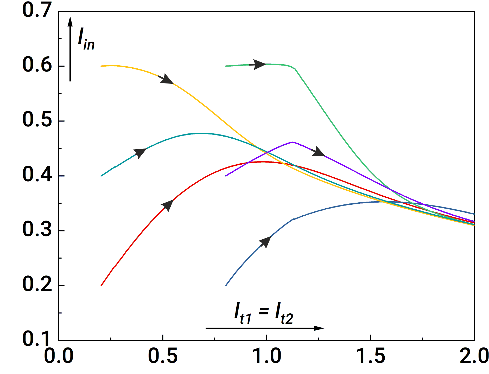
Figure 5: Gradient descent trajectories for $\max\alpha$ maximisation for different initial parameters (shown by different colors), projected onto the plane $\{l_{in};l_{t1,t2}\}$.

A visualisation of this method for different initial parameters is shown in Figure 5. We selected several initial sets of system inductances, for which $\alpha$ was calculated using (6) and maximised based on the gradient descent method. The angle $\max\alpha$ is non-monotonic with respect to the system parameters and has several local maxima. In the Figure 5 we show a section for several trajectories along which the angle $\max\alpha$ is maximised in the subspace of inductances $l_{in}$ and $l_{t1}=l_{t2}$, where the arrow indicates the path from their initial values to the optimal ones. It is seen that all curves converge at $l_{t1,2}\rightarrow 2$ (which was chosen as an upper boundary value for the inductances $l_{t1...4}$) and $l_{in}\rightarrow 0.3$, where a certain local maximum of optimisation is reached for $\max\alpha$, and therefore, for the achievable synapse weights in our system.

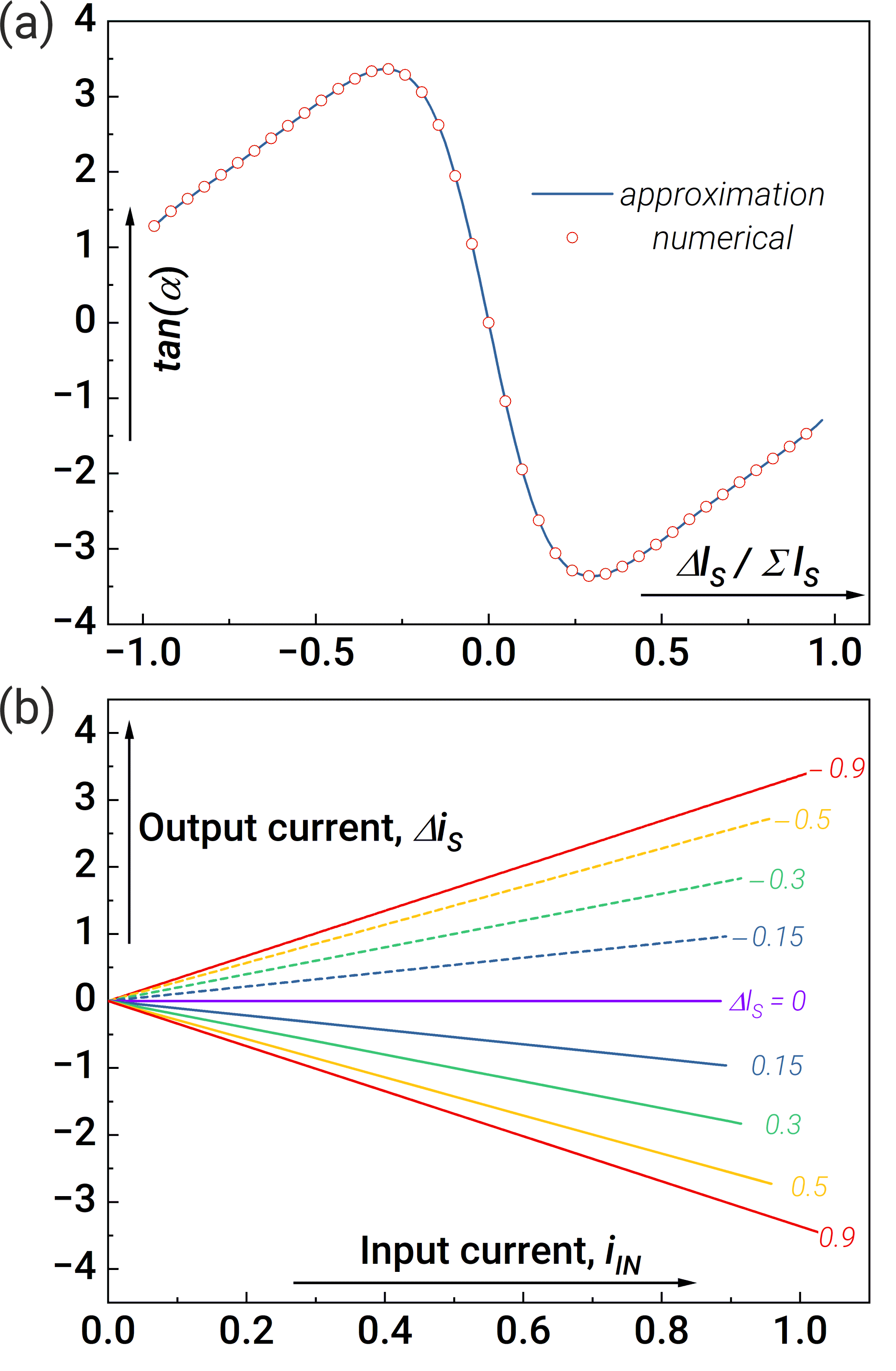
Figure 6: Demonstration of synapse capabilities after system parameters optimisation: (a) comparison of numerical and analytical calculations for the dependence of the slope angle $\alpha$ on $\Delta l_{s}$ and (b) dependence of the output current from the synapse $\Delta i_{s}$ as a function of the input current $i_{in}$. The blue line shows the result of the approximate calculation using Eqs. (6) – (8). The red circles show the result of the exact numerical calculation of the dynamics from Eq. (5). Parameters of the system are: $l_{1,2}=0.1$, $l_{in}=0.3$, $l_{t1}=l_{t2}=2$, $l_{t3}=l_{t4}=0.1$, $l_{out1,2}=0.1$, $l_{s1}+l_{s2}=3$.

Figure 6a shows $\text{tan}(\alpha)$ dependence on the inductance difference $\Delta l_{s}$ for optimal system parameters found by the gradient descent method. The good agreement between the results obtained from the exact calculation of Eq. (5) (the red circles) and by using Eqs. (6) – (8) (the blue line) indicates the validity of the approximations used. Dependencies of the synapse output current $\Delta i_{s}$ on the input current $i_{in}$ for different values of $\Delta l_{s}$ are shown in the Figure 6b.

The proposed method allows to abandon the solution of the Hamiltonian system, which is a time-consuming computational task. We reduce the optimisation problem to solving a set of algebraic equations, which significantly reduces the computational time. This approach is promising from the point of view of scaling neural networks and calculating their optimal configuration parameters.

The obtained results demonstrate that the gradient descent method can be used to optimise the parameters of a synapse connecting two neurons, Extending the applicability of the method to more complex systems consisting of a larger number of neurons and synapses is also possible, but may require additional assumptions related to mutual influence of neurons on each other (localisation approximation). Hence, the challenge of optimisation of the parameters of a large neural network will be reduced to solving local problems of finding functionals similar to Eq. (6) and then fine tuning the found solutions by the gradient descent method in a multi-parameter space.

IV Circuit structure optimisation

The performed parameter optimisation does not eliminate the signal level drop at the output neuron in the considered circuit design, Figure 2. To overcome this problem, we are developing a modification of the circuit in which the magnetic connection between the input neuron and the synapse is replaced by a galvanic connection, see Figure 7.

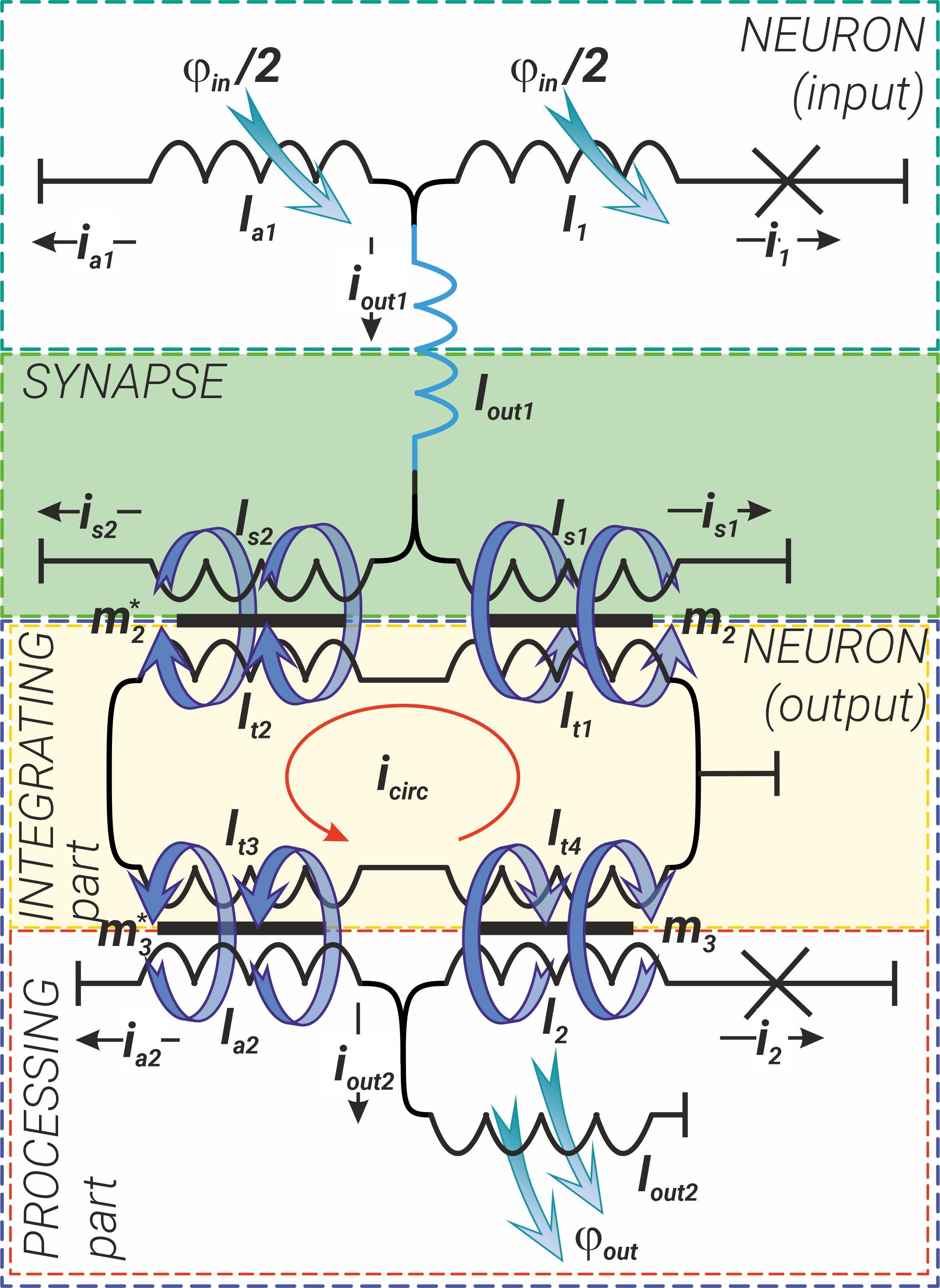
Figure 7: Schematic representation of the modified coupling between two $S_{c}$-neurons: the transformer consisting of inductances $l_{out1}$ and $l_{in}$ coupling the input neuron and the synapse (see Figure 2) is replaced by a direct coupling via the inductance $l_{out1}$ only.

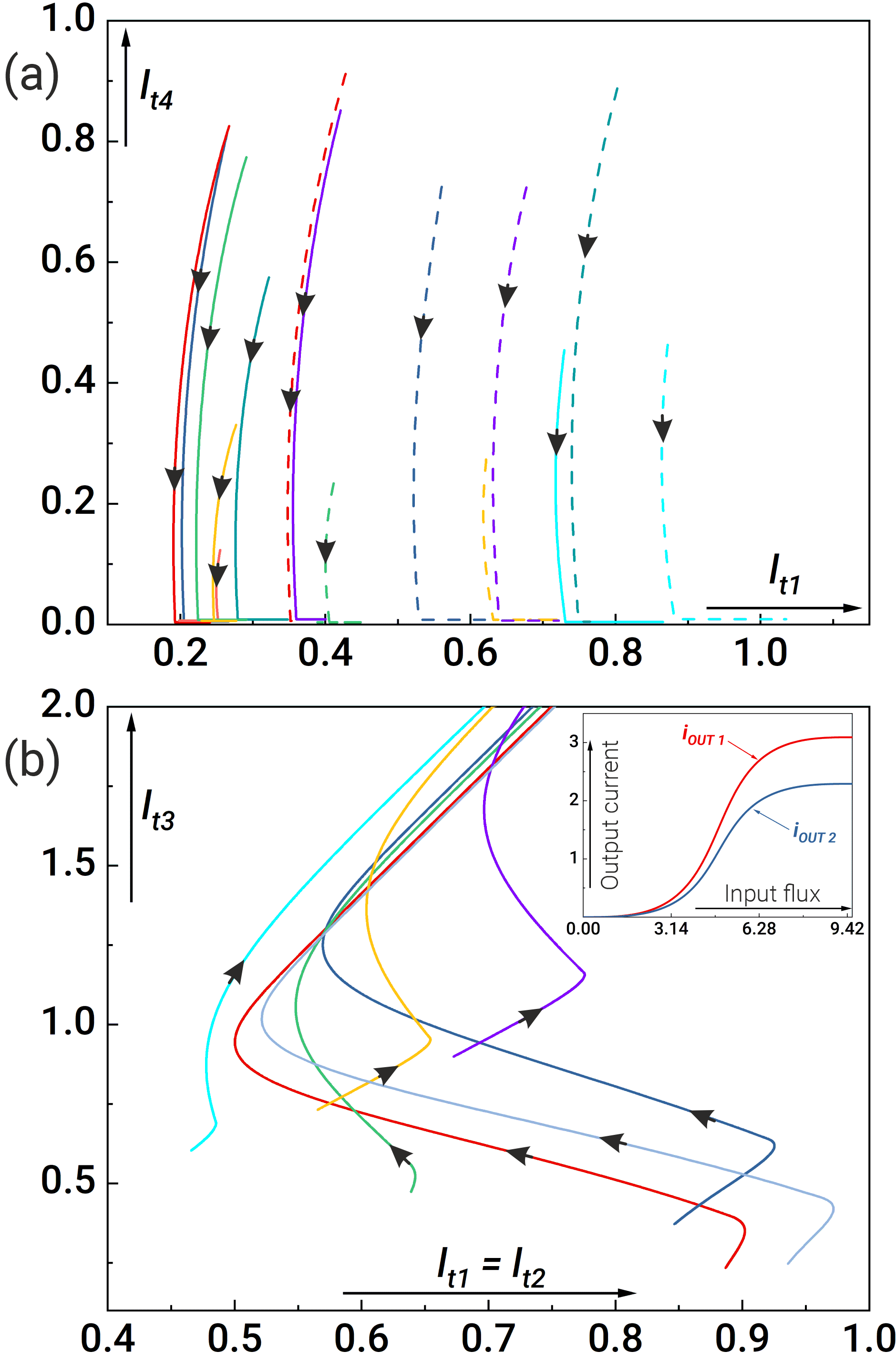
Figure 8: Projection of gradient descent trajectories for different initial parameters (each curve corresponds to its own initial values) (a) on axes $l_{t4}$ and $l_{t1}$ and (b) on axes $l_{t3}$ and $l_{t1}=l_{t2}$. The inset of figure (b) shows the transfer characteristics of the input and output neurons ($i_{out1,2}(\varphi_{in})$) with the following system parameters: $l_{1,2}=0.1$, $l_{t1}=l_{t2}=0.7$, $l_{t3}=1.5$, $l_{t4}=0.1$, $l_{out1,2}=0.1$, $\Sigma l_{s}=3$, $\Delta l_{s}=1.53$.

Within the framework of the proposed approach, gradient descent was applied to the modified scheme to solve the optimisation problems. The analysis of the system showed that the main parameters responsible for the current at the output neuron are the coupling inductances $l_{tj}$ (where $j=1,2,3,4$). Figure 8a shows that we need to minimise the value of the inductance $l_{t4}$ connecting the coupler to the Josephson arm in the output neuron. The direction of the arrows shows the path of the trajectory (from the initial value to the optimal one) for maximising the angle $\max\alpha$ during the gradient descent execution. Figure 8b shows the calculation for optimisation of the remaining coupler inductances. It can be seen that all trajectories tend to the values $l_{t3}\rightarrow 2$ and $l_{t1,2}\rightarrow 0.7$. We calculate the activation functions of the neurons shown in the inset of Figure 8b using these values. By application of the optimisation approach, we are able to significantly increase the current at the output neuron, which is important for the practical implementation of such systems.

After re-optimisation of the parameters, we re-examine the synaptic weights. We analyze the dependence of the current ratio $i_{out2}/i_{out1}$ on $\Delta l_{S}$ where the input flux reaches a plateau at $t=(t_{1}+t_{2})/2$, see Figure 9a. It can be seen, that we can adjust the sum of the inductances such that the values of the out currents at the input and output neurons coincide, see Figure 9b. Note that the output current of the output neuron can even exceed the output current of the first neuron at small values of $l_{t4}$. Thus, depending on the technological limitations, it is possible to obtain the maximum response at the output layer of the neurons.

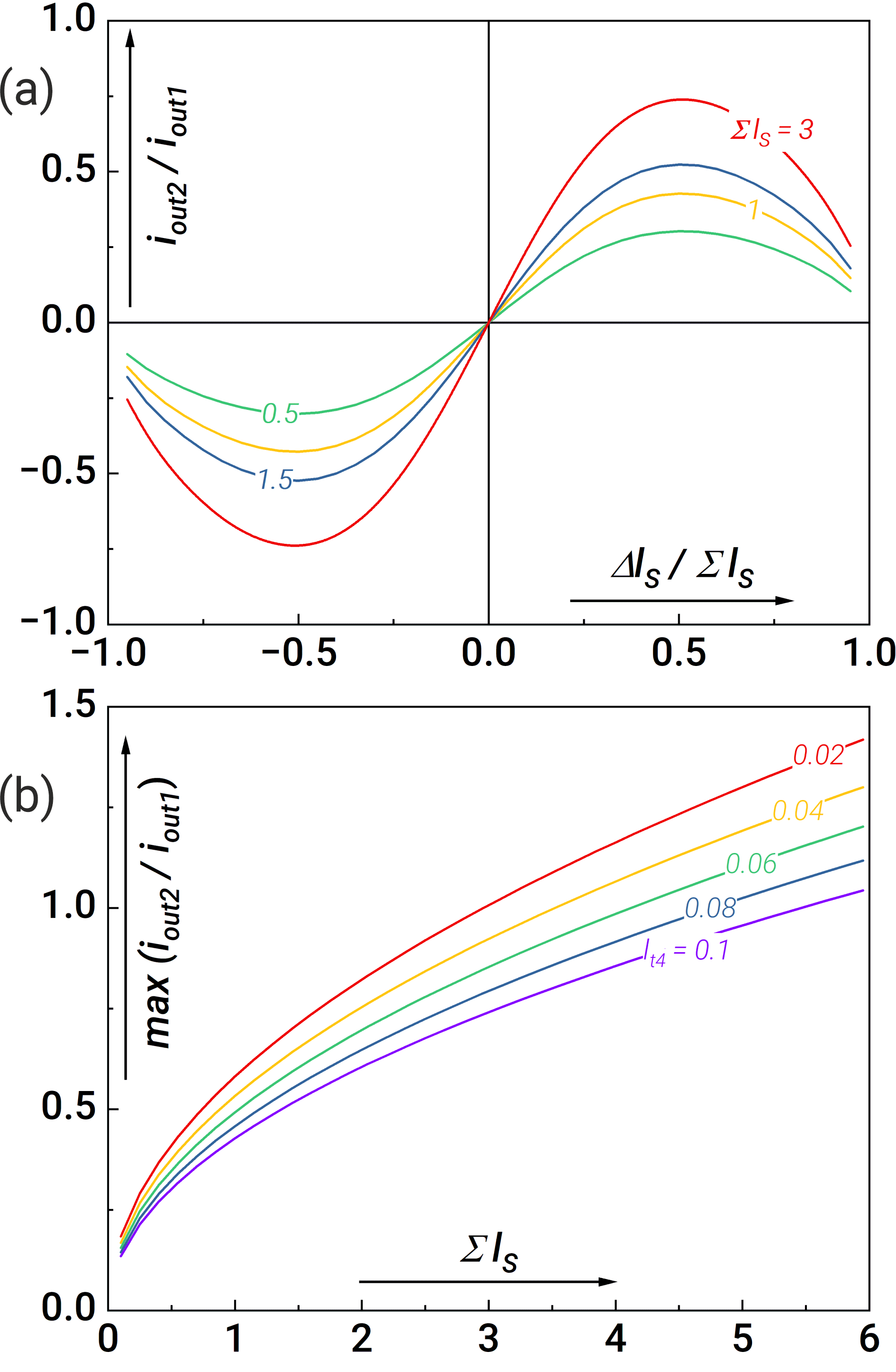
Figure 9: (a) Dependence of the current ratio $i_{out2}/i_{out1}$ at the moment when the input flux reaches a plateau at $t=(t_{1}+t_{2})/2$ on the normalised difference of the inductances of the synaptic arms for $l_{t4}=0.1$ and different values of the inductance sum. (b) Maximum ratio between output currents $i_{out2}$ and $i_{out1}$ for different values of $l_{t4}$ in dependence on the inductance sum, $\Sigma l_{s}$. Other system parameters are follows: $l_{1,2}=0.1$, $l_{t1}=l_{t2}=0.7$, $l_{t3}=1.5$, $l_{out1,2}=0.1$.

V Analog implementation of the XOR and OR logic elements

The classical XOR (logical inequality operator) element has two inputs and one output. If the input signals do not match, the output is ‘‘1’’, and ‘‘0’’ otherwise. The basic neural network implementing XOR consists of three neurons (two input neurons and one output neuron). The inputs of the neural network are supplied with signal in the form of smoothed trapezoid ‘‘1’’ or no signal ‘‘0’’, see Figure 10a, respectively. The optimisation problem is reduced to finding such parameters of the system at which the output layer neuron activates according to the XOR truth table. Similar considerations are valid for obtaining a neural network operating according to the OR gate principle.

The discussion of the neural-XOR/OR superconducting circuit based on three adiabatic neurons (shown in Figure 10b) begins with writing down the corresponding system of equations:

$$\begin{cases}(i_{1})_{in1}+(i_{a1})_{in1}+(i_{out1})_{in1}=0,\\ (i_{1})_{in2}+(i_{a1})_{in2}+(i_{out1})_{in2}=0,\\ (\varphi_{1})_{in1}-\frac{\varphi_{in1}}{2}+(i_{1}l_{1})_{in1}=(i_{out1}l_{out1})_{in1}+(i_{s1}l_{s1})_{in1}+(m_{2})_{in1}i_{circ},\\ (\varphi_{1})_{in2}-\frac{\varphi_{in2}}{2}+(i_{1}l_{1})_{in2}=(i_{out1}l_{out1})_{in2}+(i_{s1}l_{s1})_{in2}+(m_{2})_{in2}i_{circ},\\ (\varphi_{1})_{in1}-\frac{\varphi{in1}}{2}+(i_{1}l_{1})_{in1}=(i_{out1}l_{out1})_{in1}+(i_{s2}l_{s2})_{out1}-(m_{2}^{*})_{in1}i_{circ},\\ (\varphi_{1})_{in2}-\frac{\varphi_{in2}}{2}+(i_{1}l_{1})_{in2}=(i_{out1}l_{out1})_{in2}+(i_{s2}l_{s2})_{in2}-(m_{2}^{*})_{in2}i_{circ},\\ (\varphi_{1})_{in1}-\frac{\varphi_{in1}}{2}+(i_{1}l_{1})_{in1}=(i_{a1}l_{a})_{in1}+\frac{\varphi_{in1}}{2},\\ (\varphi_{1})_{in2}-\frac{\varphi_{in2}}{2}+(i_{1}l_{1})_{in2}=(i_{a1}l_{a})_{in2}+\frac{\varphi_{in2}}{2},\\ (i_{out1})_{in1}-(i_{s1})_{in1}-(i_{s2})_{in1}=0,\\ (i_{out1})_{in2}-(i_{s1})_{in2}-(i_{s2})_{in2}=0,\\ ((l_{t1})_{in1}+(l_{t2})_{in1}+(l_{t1})_{in2}+(l_{t2})_{in2}+(l_{t3})_{out1}+(l_{t4})_{out1})i_{circ}=\\ (-(i_{s1}m_{2})_{in1}-(i_{s1}m_{2})_{in2}+(i_{2}m_{3})_{out1}+(m_{2}^{*}i_{s2})_{in1}+(m_{2}^{*}i_{s2})_{in2}-(m_{3}^{*}i_{a2})_{out1}),\\ (i_{2})_{out1}+(i_{a2})_{out1}+(i_{out2})_{out1}=0,\\ (\varphi_{2})_{out1}-(m_{3})_{out1}i_{circ}+(i_{2}l_{2})_{out1}=(i_{out2}l_{out2})_{out1},\\ (\varphi_{2})_{out1}-(m_{3})_{out1}i_{circ}+(i_{2}l_{2})_{out1}=(i_{a2}l_{a2})_{out1}+(m_{3}^{*})_{out1}i_{circ},\par\end{cases}$$ (9)

where we preserve the notations according to Figure 7, but with the subscripts for the neurons in the input ($in1,2$) and output ($out1$) layers (a more detailed scheme with all designations can be found in the Supplementary Materials, see Figure S1). The input signals defined by expression (1) are denoted accordingly $\varphi_{in1,2}$.

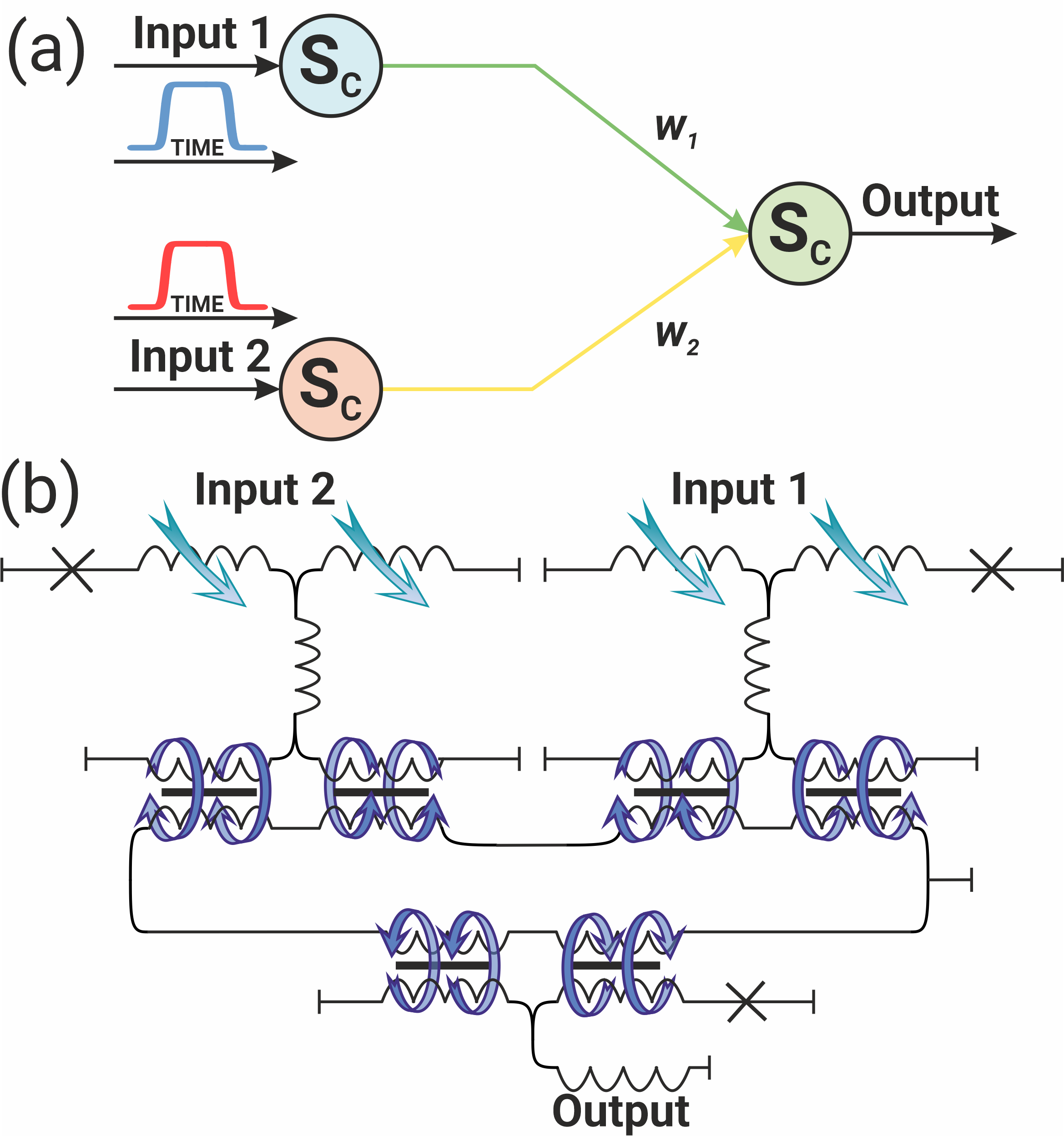
Figure 10: (a) Schematic representation of the 3-neuron XOR/OR network and (b) its superconducting implementation

Solving the optimisation problem for the system of equations (9) makes it possible to configure the neural network capable to operate both as an XOR or as an OR logic element, which is quite expected. An obvious choice for such a neural network configuration will be the choice of weight coefficients: they should be asymmetric for XOR, and, on the contrary, they should be symmetric for OR implementation. By solving the system of equations (9) describing the circuit shown in Figure 10, the truth tables for XOR/OR network implementations were obtained and presented in Figure 11. The case when there is no signal at the input of both input neurons is not shown: if there is no signal at both inputs of the circuit, there is no signal at the output as well.

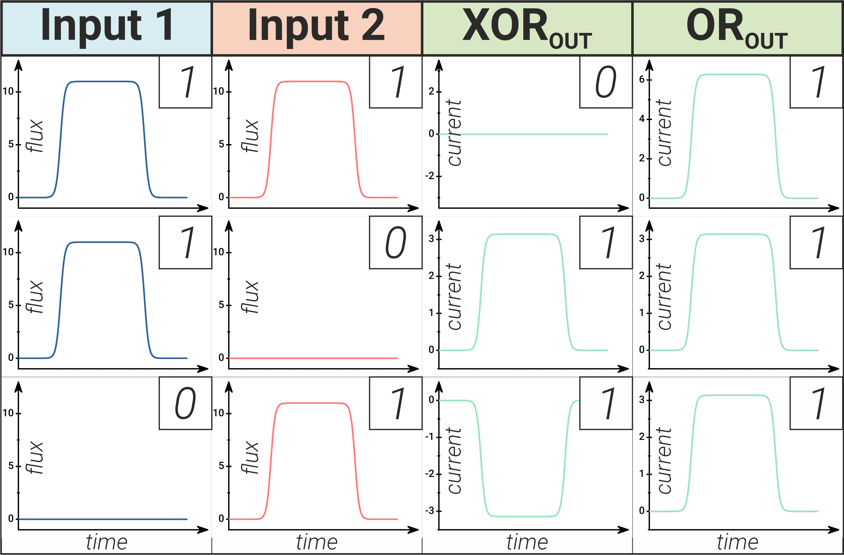
Figure 11: Demonstration of neural network operation as an XOR/OR logic gate.

Synaptic weights are asymmetric/symmetric respectively. The scheme of the neural network is shown in Figure 10.

One point is worth mentioning regarding the proposed implementations of the neural networks. Here the XOR output can be of both: positive and negative polarity (see Figure 11). The OR output with ‘‘1’’ in both inputs is twice larger than that with inputs ‘‘1’’ + ‘‘0’’ or ‘‘0’’ + ‘‘1’’ (see Figure 11). This is in contrast to the digital implementations where the output can be ‘‘0’’ or ‘‘1’’ only.

VI Conclusion

In this paper, we demonstrated optimisation algorithm for the parameters of adiabatic neural networks. The algorithm allowed us to find the optimal values for operation of the circuits with different combinations of synapses and neurons, including the ones mimicking logical XOR and OR elements. In addition, a generalisation of this algorithm to neural networks of higher dimensionality consisting of superconducting $S_{c}$-neurons and synapses was discussed.

It should be noted that even in the development of such simple neural networks, we faced a significant signal decay problem. For larger neural networks the solution may imply an addition of magnetic flux amplifiers (boosters), well-known in adiabatic superconducting logic Mizushima et al. (2023). An utilization of analogue-digital (and, apparently, optical-superconductor) approach for the network implementations is another option.

Regarding the experimental feasibility of the presented schemes, there are a number of experimental works Ionin et al. (2023a, b); He et al. (2020); Takeuchi et al. (2023) using a similar technique for the fabrication of Josephson junctions and demonstrating their critical currents in the range of 50 to 150 $\mu$A, corresponding to characteristic values of inductance magnitudes at the level of 2.2 – 6.6 pH. This confirms the experimental feasibility of the design considerations presented.

VII ACKNOWLEDGMENTS

The development of the main concept was carried out with the financial support of the Strategic Academic Leadership Program ‘‘Priority-2030’’ (grant from NITU ‘‘MISIS’’ No. K2-2022-029). The development of the method of analysing for the evolution of the adiabatic logic cells was carried out with the support of the Grant of the Russian Science Foundation No. 22-72-10075. A.S. is grateful to the grant 22-1-3-16-1 from the Foundation for the Advancement of Theoretical Physics and Mathematics ‘‘BASIS’’. The work of M.B. and I.S. was supported by Rosatom in the framework of the Roadmap for Quantum computing (Contract No. 868-1.3-15/15-2021 dated October 5).

VIII Supplementary Materials

VIII.1 Analycal expressions of coefficients for ‘‘equations of motion’’

The analytical representation of the coefficients for the ’’equations of motion’’ of the composite system (2) is given below:

$$\begin{split}\kappa_{1}^{(2)}&=\kappa_{2}^{(1)}=1/(l_{1}l_{a2}l_{o}^{2}l_{ps2}m_{1})(l_{a2}m_{2p}(l_{ao1}l_{ps2}m_{2}+l_{ao1}l_{inp}m_{2p}-l_{r1}m_{2p})(-l_{k}l_{o}l_{out1}+\\ &l_{ao2}(l_{ps2}m_{2}-l_{ps1}m_{2}^{*})(-m_{1}^{2}m_{2p}+l_{out1}(2l_{p}m_{2}+l_{s2}m_{2}+l_{in}m_{2p}+l_{p}m_{2}^{*})))\\ &(l_{a2}l_{at2}m_{3}+(l_{ao2}-l_{2}l_{at2})m_{3}^{*})+l_{o}l_{ps2}(m_{1}^{2}m_{2p}-l_{out1}(l_{s2}m_{2}+l_{in}m_{2p}+l_{p}(2m_{2}+m_{2}^{*})))\\ &(l_{ao2}m_{3}^{*}+(l_{a2}m_{3}-l_{2}m_{3}^{*})(l_{out2}+l_{a2}(l_{a2}m_{3}-l_{2}m_{3}^{*})))),\\ \kappa_{1}^{(in)}&=(l_{w}-(l_{1}-l_{a1})l_{a2}(-m_{1}^{2}m_{2p}(-l_{ps2}l_{x}+l_{y}+l_{ao2}m_{2p}m_{2}^{*})+l_{out1}(l_{ps1}l_{s2}l_{x}m_{2}+l_{ps2}l_{y}m_{2}\\ &-l_{is}l_{s2}l_{x}m_{2p}+l_{inp}l_{y}m_{2p}+l_{p}l_{x}(l_{ps1}m_{2}-l_{is}m_{2p})+l_{ao2}m_{2p}(-l_{ps1}m_{2}+\\ &+l_{is}m_{2p})m_{2}^{*})))/(2l_{1}l_{w}),\\ \kappa_{2}^{(1)}&=-((l_{a1}l_{q}m_{1}m_{2p}(l_{ps2}m_{2}-l_{ps1}m_{2}^{*})(l_{a2}m_{3}+l_{out2}m_{3p}))/((l_{r1}(l_{q}-l_{a2}l_{y})m_{2p}+\\ &l_{ao1}(l_{ps1}l_{q}m_{2}+l_{a2}l_{ps2}l_{y}m_{2}-l_{is}l_{q}m_{2p}+l_{a2}l_{inp}l_{y}m_{2p}))(-l_{2}l_{at2}l_{f}-l_{a2}l_{out2}l_{ps2}l_{t}+\\ &l_{a2}l_{out2}m_{2p}m_{2}^{*}+l_{a2}l_{ps2}m_{3}^{2}+l_{out2}l_{ps2}m_{3p}^{2}+l_{2}l_{ps2}m_{3}^{*2})))\\ \kappa_{2}^{(in)}&=-(((l_{1}-l_{a1})l_{q}m_{1}m_{2p}(l_{ps2}m_{2}-l_{ps1}m_{2}^{*})(l_{a2}m_{3}+l_{out2}m_{3p}))/(2(l_{r1}(l_{q}-l_{a2}l_{y})m_{2p}+\\ &l_{ao1}(l_{ps1}l_{q}m_{2}+l_{a2}l_{ps2}l_{y}m_{2}-l_{is}l_{q}m_{2p}+l_{a2}l_{inp}l_{y}m_{2p}))(-l_{2}l_{at2}l_{f}-l_{a2}l_{out2}l_{ps2}l_{t}+\\ &l_{a2}l_{out2}m_{2p}m_{2}^{*}+l_{a2}l_{ps2}m_{3}^{2}+l_{out2}l_{ps2}m_{3p}^{2}+l_{2}l_{ps2}m_{3}^{*2}))),\\ \kappa_{in}^{(1)}&=(l_{a1}m_{1}(l_{2}l_{at2}(-l_{ps}l_{t}+m_{2p}^{2})+l_{a2}l_{out2}(-l_{ps}l_{t}+m_{2p}^{2})+l_{a2}l_{ps}m_{3}^{2}+l_{out2}l_{ps}m_{3p}^{2}+\\ &l_{2}l_{ps}m_{3}^{*2}))/l_{g},\\ \kappa_{in}^{(1)}&=(l_{a1}m_{1}(l_{2}l_{at2}(-l_{ps}l_{t}+m_{2p}^{2})+l_{a2}l_{out2}(-l_{ps}l_{t}+m_{2p}^{2})+l_{a2}l_{ps}m_{3}^{2}+l_{out2}l_{ps}m_{3p}^{2}+\\ &l_{2}l_{ps}m_{3}^{*2}))/l_{g},\\ \end{split}$$

$$\begin{split}\kappa_{in}^{(2)}&=-((l_{ao1}(l_{ps2}m_{2}-l_{ps1}m_{2}^{*})(l_{a2}m_{3}+l_{out2}m_{3p}))/l_{g}),\\ \kappa_{in}^{(in)}&=-(((l_{1}-l_{a1})m_{1}(l_{a2}(l_{out2}l_{ps}l_{t}-l_{out2}m_{2p}^{2}-l_{ps}m_{3}^{2})-l_{out2}l_{ps}m_{3p}^{2}+l_{2}(l_{at2}l_{ps}l_{t}-\\ &l_{at2}m_{2p}^{2}-l_{ps}m_{3}^{*2})))/l_{d}),\\ \kappa^{(1)}_{s}&=(l_{a1}m_{1}(l_{a2}l_{out2}(-l_{s1}l_{t}+l_{s2}l_{t}+m_{2}m_{2p}-m_{2p}m_{2}^{*})+l_{2}l_{at2}(-l_{s1}l_{t}+l_{s2}l_{t}+m_{2}^{2}-\\ &m_{2}^{*2})+l_{a2}(l_{s1}-l_{s2})m_{3}^{2}+l_{out2}(l_{s1}-l_{s2})m_{3p}^{2}+l_{2}(l_{s1}-l_{s2})m_{3}^{*2}))/l_{g},\\ \kappa^{(2)}_{s}&=(l_{ao1}(2l_{in}+3l_{p}+l_{s2})m_{2}-2l_{r1}m_{2p}+l_{ao1}(2l_{in}+3l_{p}+l_{s1})m_{2}^{*})(l_{a2}m_{3}+l_{out2}m_{3p})/l_{g}\\ \kappa^{(in)}_{s}&=-(((l_{1}-l_{a1})m_{1}(l_{2}l_{at2}(l_{s1}l_{t}-l_{s2}l_{t}-m_{2}^{2}+m_{2}^{*2})+l_{a2}l_{out2}(l_{s1}l_{t}-l_{s2}l_{t}-m_{2}^{2}+m_{2}^{*2})+\\ &l_{a2}(-l_{s1}+l_{s2})m_{3}^{2}+l_{out2}(-l_{s1}+l_{s2})m_{3p}^{2}+l_{2}(-l_{s1}+l_{s2})m_{3}^{*2}))/l_{d}).\\ \end{split}$$

The following is a list of the notations used in the given coefficients:

$$l_{t}=l_{t1}+l_{t2}+l_{t3}+l_{t4},$$

$$l_{ao1}=l_{1}l_{at1}+l_{a1}l_{out1},\quad l_{ao2}=l_{2}l_{at2}+l_{a2}l_{out2},$$

$$l_{r1}=(l_{1}+l_{a1})m_{1}^{2},\quad l_{ps1}=l_{p}+l_{s1},\quad l_{ps2}=l_{p}+l_{s2},$$

$$m_{2p}=m_{2}+m_{2}^{*},\quad m_{3p}=m_{3}+m_{3}^{*},$$

$$l_{ps1}=l_{p}+l_{s1},\quad l_{ps2}=l_{p}+l_{s2},$$

$$l_{x}=l_{2}l_{at2}l_{t}+l_{a2}l_{out2}l_{t}-l_{a2}m_{3}^{2}-l_{out2}m_{3p}^{2}-l_{2}m_{3}^{*2},$$

$$\begin{split}l_{y}=l_{ao2}m_{2}m_{2p}+&l_{a2}l_{ps1}(-l_{out2}l_{t}+m_{3}^{2})+l_{out2}l_{ps1}m_{3p}^{2}+\\ &l_{2}l_{ps1}(-l_{at2}l_{t}+m_{3}^{*2})\end{split}$$

$$l_{inp}=l_{in}+l_{p},\quad l_{is}=l_{in}+2l_{p}+l_{s1},$$

$$l_{q}=l_{a2}(l_{ps2}l_{x}-l_{ao2}m_{2p}m_{2}^{*}),$$

$$\begin{split}l_{w}=l_{r1}(-l_{q}+&l_{a2}l_{y})m_{2p}-l_{ao1}(l_{ps1}l_{q}m_{2}+l_{a2}l_{ps2}l_{y}m_{2}\\ &-l_{is}l_{q}m_{2p}+l_{a2}l_{inp}l_{y}m_{2p})\end{split}$$

$$l_{j}=l_{out12}l_{p},\quad l_{ps}=2l_{p}+l_{s1}+l_{s2},$$

$$l_{k}=3l_{p}^{2}+l_{in}l_{ps}+2l_{p}l_{s12}+l_{s1}l_{s2},$$

$$l_{b}=2l_{j}+l_{a2}l_{out1}l_{ps}+l_{out12}l_{s12},$$

$$l_{s12}=l_{s1}+l_{s2},\quad l_{at1}=l_{a1}+l_{out1},\quad l_{at2}=l_{a2}+l_{out2},$$

$$l_{out12}=l_{out1}l_{out2},\quad l_{ps12}=l_{ps1}+l_{ps2},$$

$$\begin{split}l_{u}=&l_{a2}(2l_{j}(-l_{s12}l_{t}+m_{2}^{2}+m_{2}m_{2}^{*}+m_{2}^{*2})+l_{out12}(-3l_{p}^{2}l_{t}-l_{in}l_{ps}l_{t}-l_{s1}l_{s2}l_{t}+l_{s2}m_{2}^{2}+l_{in}m_{2p}^{2}+l_{s1}m_{2}^{*2})+l_{k}l_{out1}m_{3}^{2}+\\ &m_{1}^{2}(l_{out2}l_{ps}l_{t}-l_{out2}m_{2p}^{2}-l_{ps}m_{3}^{2}))+l_{out2}(l_{k}l_{out1}-l_{ps}m_{1}^{2})m_{3p}^{2}+l_{2}(-l_{b}l_{in}l_{t}-l_{t}(3l_{out12}l_{p}^{2}+\\ &2l_{j}l_{s12}+l_{out12}l_{s1}l_{s2}-l_{out2}l_{ps}m_{1}^{2})+(2l_{j}+l_{out12}l_{s2}-l_{out2}m_{1}^{2})m_{2}^{2}+l_{in}l_{out12}m_{2p}^{2}+m_{2}^{*}(2l_{j}m_{2p}+\\ &l_{out12}l_{s1}m_{2}^{*}-l_{out2}m_{1}^{2}(2m_{2}+m_{2}^{*}))+l_{a2}(m_{1}^{2}(l_{ps}l_{t}-m_{2p}^{2})+l_{out1}(-3l_{p}^{2}l_{t}-l_{s1}l_{s2}l_{t}+l_{s2}m_{2}^{2}+\\ &l_{in}m_{2p}^{2}+l_{s1}m_{2}^{*2}+2l_{p}(-l_{s12}l_{t}+m_{2}^{2}+m_{2}m_{2}^{*}+m_{2}^{*2})))+(l_{k}l_{out1}-l_{ps}m_{1}^{2})m_{3}^{*2}),\\ l_{e}=&l_{out2}m_{1}^{2}(2l_{p}l_{t}+l_{s12}l_{t}-m_{2p}^{2})+2l_{j}(-l_{s12}l_{t}+m_{2}^{2}+m_{2}m_{2}^{*}+m_{2}^{*2})+l_{out12}(-3l_{p}^{2}l_{t}+l_{s2}m_{2}^{2}+l_{s1}(-l_{s2}l_{t}+m_{2}^{*2}))+\\ &l_{a1}l_{out2}(-3l_{p}^{2}l_{t}+l_{s2}m_{2}^{2}+l_{s1}(-l_{s2}l_{t}+m_{2}^{*2})+2l_{p}(-l_{s12}l_{t}+m_{2}^{2}+m_{2}m_{2}^{*}+m_{2}^{*2}))+(l_{at1}(3l_{p}^{2}+2l_{p}l_{s12}+l_{s1}l_{s2})-\\ &l_{ps}m_{1}^{2})m_{3}^{2}+l_{in}(-2l_{j}l_{t}-l_{out12}l_{s12}l_{t}+l_{out12}m_{2p}^{2}+l_{a1}l_{out2}(-l_{ps}l_{t}+m_{2p}^{2})+l_{at1}l_{ps}m_{3}^{2}),\\ l_{h}=&-l_{b}l_{in}l_{t}-l_{a2}l_{out1}(3l_{p}^{2}+2l_{p}l_{s12}+l_{s1}l_{s2})l_{t}+l_{t}(3l_{out12}l_{p}^{2}+2l_{j}l_{s12}+l_{out12}l_{s1}l_{s2}-l_{at2}l_{ps}m_{1}^{2})+(2l_{j}+l_{out12}l_{s2}+\\ &l_{a2}l_{out1}(2l_{p}+l_{s2})-l_{at2}m_{1}^{2})m_{2}^{2}+l_{in}(l_{a2}l_{out1}+l_{out12})m_{2p}^{2}-2(l_{j}+l_{a2}l_{out1}l_{p}-l_{at2}m_{1}^{2})m_{2}m_{2}^{*}+(2l_{j}+l_{out12}l_{s1}+\\ &l_{a2}l_{out1}(2l_{p}+l_{s1})-l_{at2}m_{1}^{2})m_{2}^{*2}+l_{a1}l_{at2}(-3l_{p}^{2}l_{t}+l_{in}l_{ps}l_{t}-l_{s1}l_{s2}l_{t}+l_{s2}m_{2}^{2}-l_{in}m_{2p}^{2}+l_{s1}m_{2}^{*2}+2l_{p}(-l_{s12}l_{t}+m_{2}^{2}+\\ &m_{2}m_{2}^{*}+m_{2}^{*2}))+l_{a1}l_{k}m_{3}^{*2}+(l_{k}l_{out1}-l_{ps}m_{1}^{2})m_{3}^{*2}\\ l_{g}=&l_{a1}l_{u}+l_{1}(l_{a2}l_{e}+l_{2}l_{h}+(2l_{in}l_{j}+3(l_{out12}+l_{a1}l_{out2})l_{p}^{2}+l_{a1}l_{in}l_{out2}l_{ps}+2l_{j}l_{s12}+l_{in}l_{out12}l_{s12}+2l_{a1}l_{out2}l_{p}l_{s12}+\\ &l_{out12}l_{s1}l_{s2}+l_{a1}l_{out2}l_{s1}l_{s2}-l_{out2}l_{ps}m_{1}^{2})m_{3}^{2}+2l_{out2}(l_{at1}l_{k}-l_{ps}m_{1}^{2})m_{3}m_{3}^{*}+l_{out2}(l_{at1}l_{k}-l_{ps}m_{1}^{2})m_{3}^{*2}),\\ l_{d}=&2(l_{a1}l_{u}+l_{1}(l_{2}l_{h}+(2l_{in}l_{j}+3(l_{out12}+l_{a1}l_{out2})l_{p}^{2}+2l_{j}l_{s12}+l_{in}l_{out12}l_{s12}+l_{out12}l_{s1}l_{s2}+l_{a1}l_{out2}(l_{in}l_{ps}+2l_{p}l_{s12}+\\ &l_{s1}l_{s2})-l_{out2}l_{ps}m_{1}^{2})m_{3}^{2}-l_{a2}(l_{in}(2l_{j}+l_{a1}l_{out2}l_{ps}+l_{out12}l_{s12})l_{t}+2l_{j}(l_{s12}l_{t}-m_{2}^{2})+l_{out2}m_{1}^{2}(-l_{ps}l_{t}+m_{2}^{2})-\\ &l_{in}(l_{out12}+l_{a1}l_{out2})m_{2p}^{2}+l_{out12}(3l_{p}^{2}l_{t}+l_{s1}l_{s2}l_{t}-l_{s2}m_{2}^{2}-l_{s1}m_{2}^{*2})+l_{a1}l_{out2}(3l_{p}^{2}l_{t}+2l_{p}l_{s12}l_{t}+l_{s1}l_{s2}l_{t}-l_{s2}m_{2}^{2}-\\ &2l_{p}m_{2}m_{2p}-(2l_{p}+l_{s1})m_{2}^{*2})-m_{2}^{*}(2l_{j}(m_{2}-m_{2}^{*})+l_{out2}m_{1}^{2}(2m_{2}+m_{2}^{*}))-l_{at1}l_{k}m_{3}^{2}+l_{ps}m_{1}^{2}m_{3}^{2})+2l_{out2}(l_{at1}l_{k}-\\ &l_{ps}m_{1}^{2})m_{3}m_{3}^{*}+l_{out2}(l_{at1}l_{k}-l_{ps}m_{1}^{2})m_{3}^{*2})),\\ l_{f}=&l_{ps2}l_{t}-m_{2p}m_{2}^{*},l_{o}=l_{2}l_{at2}l_{f}+l_{a2}l_{out2}l_{ps2}l_{t}-l_{a2}l_{out2}m_{2p}m_{2}^{*}-l_{a2}l_{ps2}m_{3}^{2}-l_{out2}l_{ps2}m_{3p}^{2}-l_{2}l_{ps2}m_{3}^{*2}\end{split}$$

VIII.2 Hamiltonian formalism for two coupled neurons

The study of the dynamic properties of connected neurons can also be carried out within the framework of the Hamiltonian formalism. Herewith our system can be represented as two bound particles with momenta $p_{n}=c_{n}\dot{\varphi_{n}}$, and therefore the motion of particles obeys the classical Hamilton’s equations:

$$\begin{cases}\dot{\varphi_{n}}=\frac{\partial H}{\partial p_{n}},\\ \dot{p_{n}}=-\frac{\partial H}{\partial\varphi_{n}},\end{cases}$$ (10)

where $H$ is a Hamiltonian (an integral of motion).

By integrating the system (10) we can find the momentum parts of the Hamiltonian, which have the standard form $p^{2}_{n}/(2c_{n})$. Also from Eq. (5) it can be seen that $\dot{p_{n}}=i_{n}-i_{C_{n}}\sin\varphi_{n}$, therefore using the Hamiltonian’s feature $\kappa\equiv\kappa_{1}^{(2)}=\kappa_{2}^{(1)}$ one gets the form:

$$H=\sum_{n=1,2}\left(H_{\omega_{n}}-i_{C_{n}}\cos\varphi_{n}\right)+\kappa\varphi_{1}\varphi_{2}-$$ (11)

$$\left(\frac{\left(\kappa_{1}^{(in)}\right)^{2}}{2\kappa_{1}^{(1)}}+\frac{\left(\kappa_{2}^{(in)}\right)^{2}}{2\kappa_{2}^{(2)}}\right)\varphi^{2}_{in}.$$

Here the first term defines the Hamiltonians of individual neurons

$$H_{\omega_{n}}=\frac{p^{2}_{n}}{2c_{n}}+\frac{\omega^{2}_{n}}{2}\left(\varphi_{n}+\frac{\kappa_{n}^{(in)}}{\kappa_{n}^{(n)}}\varphi_{in}\right)^{2},\omega^{2}_{n}=\kappa_{n}^{(n)}\;(n=1,2).$$

The second term in Eq. (11) defines the interaction between neurons, and the last term is responsible for the dynamic control of neurons by the external magnetic flux $\varphi_{in}$ according to (1).

Using the example of two interacting neurons within the framework of the Hamiltonian formalism, it is clearly seen that the dynamic processes in the system resemble two interacting nonlinear oscillators, the coupling strength of which is linear relative to the phases at each of the Josephson contacts. Using this approach, the numerical analysis of the system is reduced to solving coupled differential equations of the first order (in contrast to (5), where it is necessary to solve a system of differential equations of the second order), which greatly simplifies further consideration of more complex systems of coupled neurons and synapses.

VIII.3 Superconducting XOR/OR network scheme with notations

Here is a more detailed scheme of the XOR/OR network with all the notations used in the system of equations (9) – Figure 12.

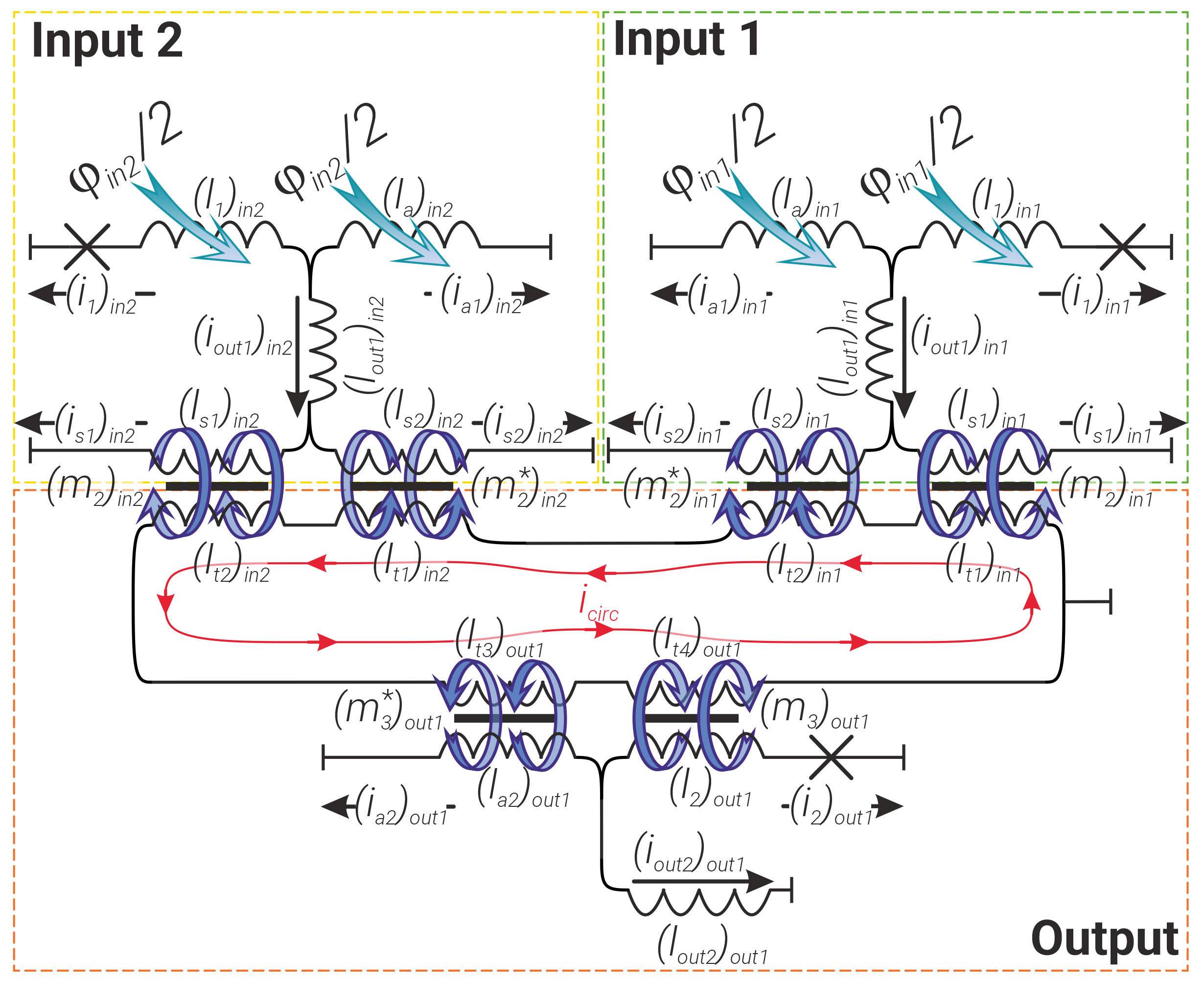
Figure 12: Schematic representation of the 3-neuron XOR/OR network in its superconducting implementation

References

• Zbontar and LeCun (2016) J. Zbontar and Y. LeCun, J. Mach. Learn. Res. 17, 2287 (2016).
• Tolosana et al. (2018) R. Tolosana, R. Vera-Rodriguez, J. Fierrez,  and J. Ortega-Garcia, IEEE Access 6, 5128 (2018).
• Kaya and Bilge (2019) M. Kaya and H. Ş. Bilge, Symmetry 11, 1066 (2019).
• Ruiz et al. (2020) V. Ruiz, I. Linares, A. Sanchez,  and J. F. Velez, Neurocomputing 374, 30 (2020).
• Wang and Deng (2021) M. Wang and W. Deng, Neurocomputing 429, 215 (2021).
• Ilina et al. (2022) O. Ilina, V. Ziyadinov, N. Klenov,  and M. Tereshonok, Symmetry 14, 1391 (2022).
• Le Gallo et al. (2023) M. Le Gallo, R. Khaddam-Aljameh, M. Stanisavljevic, A. Vasilopoulos, B. Kersting, M. Dazzi, G. Karunaratne, M. Brändli, A. Singh, S. M. Mueller, et al., Nature Electronics , 1 (2023).
• Modha et al. (2023) D. S. Modha, F. Akopyan, A. Andreopoulos, R. Appuswamy, J. V. Arthur, A. S. Cassidy, P. Datta, M. V. DeBole, S. K. Esser, C. O. Otero, et al., Science 382, 329 (2023).
• Kumar (2013) S. Kumar, Qualcomm OnQ Blog , 1 (2013).
• Prezioso et al. (2015) M. Prezioso, F. Merrikh-Bayat, B. Hoskins, G. C. Adam, K. K. Likharev,  and D. B. Strukov, Nature 521, 61 (2015).
• Bose et al. (2017) S. K. Bose, J. B. Mallinson, R. M. Gazoni,  and S. A. Brown, IEEE Transactions on Electron Devices 64, 5194 (2017).
• Davies et al. (2018) M. Davies, N. Srinivasa, T.-H. Lin, G. Chinya, Y. Cao, S. H. Choday, G. Dimou, P. Joshi, N. Imam, S. Jain, et al., IEEE Micro 38, 82 (2018).
• Cheng et al. (2018) R. Cheng, U. S. Goteti,  and M. C. Hamilton, Journal of Applied Physics 124, 152126 (2018).
• Jeong and Shi (2018) H. Jeong and L. Shi, Journal of Physics D: Applied Physics 52, 023003 (2018).
• DeBole et al. (2019) M. V. DeBole, B. Taba, A. Amir, F. Akopyan, A. Andreopoulos, W. P. Risk, J. Kusnitz, C. O. Otero, T. K. Nayak, R. Appuswamy, et al., Computer 52, 20 (2019).
• Arute et al. (2019) F. Arute, K. Arya, R. Babbush, D. Bacon, J. C. Bardin, R. Barends, R. Biswas, S. Boixo, F. G. Brandao, D. A. Buell, et al., Nature 574, 505 (2019).
• Berggren et al. (2020) K. Berggren, Q. Xia, K. K. Likharev, D. B. Strukov, H. Jiang, T. Mikolajick, D. Querlioz, M. Salinga, J. R. Erickson, S. Pi, et al., Nanotechnology 32, 012002 (2020).
• Wan et al. (2022) W. Wan, R. Kubendran, C. Schaefer, S. B. Eryilmaz, W. Zhang, D. Wu, S. Deiss, P. Raina, H. Qian, B. Gao, et al., Nature 608, 504 (2022).
• Feldmann et al. (2019) J. Feldmann, N. Youngblood, C. D. Wright, H. Bhaskaran,  and W. H. Pernice, Nature 569, 208 (2019).
• Jha et al. (2022) A. Jha, C. Huang, H.-T. Peng, B. Shastri,  and P. R. Prucnal, Journal of Lightwave Technology 40, 2901 (2022).
• Singh and Zheludev (2014) R. Singh and N. Zheludev, Nature photonics 8, 679 (2014).
• Fan et al. (2018) L. Fan, C.-L. Zou, R. Cheng, X. Guo, X. Han, Z. Gong, S. Wang,  and H. X. Tang, Science advances 4, eaar4994 (2018).
• Gu et al. (2017) X. Gu, A. F. Kockum, A. Miranowicz, Y.-x. Liu,  and F. Nori, Physics Reports 718, 1 (2017).
• Berman et al. (2006) O. L. Berman, Y. E. Lozovik, S. L. Eiderman,  and R. D. Coalson, Physical Review B 74, 092505 (2006).
• Shainline et al. (2017) J. M. Shainline, S. M. Buckley, R. P. Mirin,  and S. W. Nam, Physical Review Applied 7, 034013 (2017).
• Shainline et al. (2018) J. M. Shainline, S. M. Buckley, A. N. McCaughan, J. Chiles, A. Jafari-Salim, R. P. Mirin,  and S. W. Nam, Journal of Applied Physics 124 (2018).
• Shainline et al. (2019) J. M. Shainline, S. M. Buckley, A. N. McCaughan, J. T. Chiles, A. Jafari Salim, M. Castellanos-Beltran, C. A. Donnelly, M. L. Schneider, R. P. Mirin,  and S. W. Nam, Journal of Applied Physics 126 (2019).
• Schneider et al. (2022) M. Schneider, E. Toomey, G. Rowlands, J. Shainline, P. Tschirhart,  and K. Segall, Superconductor Science and Technology 35, 053001 (2022).
• Crotty et al. (2010) P. Crotty, D. Schult,  and K. Segall, Physical Review E 82, 011914 (2010).
• Russek et al. (2016) S. E. Russek, C. A. Donnelly, M. L. Schneider, B. Baek, M. R. Pufall, W. H. Rippard, P. F. Hopkins, P. D. Dresselhaus,  and S. P. Benz, in 2016 IEEE International Conference on Rebooting Computing (ICRC) (IEEE, 2016) pp. 1–5, san Diego, CA, USA, 17 –19 October 2016.
• Schneider et al. (2018) M. L. Schneider, C. A. Donnelly, S. E. Russek, B. Baek, M. R. Pufall, P. F. Hopkins, P. D. Dresselhaus, S. P. Benz,  and W. H. Rippard, Science advances 4, e1701329 (2018).
• Toomey et al. (2020) E. Toomey, K. Segall, M. Castellani, M. Colangelo, N. Lynch,  and K. K. Berggren, Nano Letters 20, 8059 (2020).
• Ishida et al. (2021) K. Ishida, I. Byun, I. Nagaoka, K. Fukumitsu, M. Tanaka, S. Kawakami, T. Tanimoto, T. Ono, J. Kim,  and K. Inoue, IEEE Micro 41, 19 (2021).
• Zhang et al. (2021) H. Zhang, C. Gang, C. Xu, G. Gong,  and H. Lu, IEEE Transactions on Emerging Topics in Computational Intelligence 7, 271 (2021).
• Semenov et al. (2021) V. K. Semenov, E. B. Golden,  and S. K. Tolpygo, IEEE Transactions on Applied Superconductivity 32, 1 (2021).
• Casaburi and Hadfield (2022) A. Casaburi and R. H. Hadfield, Nature Electronics 5, 627 (2022).
• Feldhoff and Toepfer (2024) F. Feldhoff and H. Toepfer, IEEE Transactions on Applied Superconductivity 34, 1 (2024).
• Siddiqi (2021) I. Siddiqi, Nature Reviews Materials 6, 875 (2021).
• Vozhakov et al. (2022) V. A. Vozhakov, M. V. Bastrakova, N. V. Klenov, I. I. Soloviev, W. V. Pogosov, D. V. Babukhin, A. A. Zhukov,  and A. M. Satanin, Phys.-Uspekhi 65, 457 (2022).
• Calzona and Carrega (2022) A. Calzona and M. Carrega, Superconductor Science and Technology 36, 023001 (2022).
• Segall et al. (2017) K. Segall, M. LeGro, S. Kaplan, O. Svitelskiy, S. Khadka, P. Crotty,  and D. Schult, Physical Review E 95, 032220 (2017).
• Feldhoff and Toepfer (2021) F. Feldhoff and H. Toepfer, IEEE Transactions on Applied Superconductivity 31, 1 (2021).
• Goteti and Dynes (2021) U. S. Goteti and R. C. Dynes, Journal of Applied Physics 129, 073901 (2021).
• Chalkiadakis and Hizanidis (2022) D. Chalkiadakis and J. Hizanidis, Physical Review E 106, 044206 (2022).
• Schegolev et al. (2023) A. E. Schegolev, N. V. Klenov, G. I. Gubochkin, M. Y. Kupriyanov,  and I. I. Soloviev, Nanomaterials 13, 2101 (2023).
• Crotty et al. (2023) P. Crotty, K. Segall,  and D. Schult, IEEE Transactions on Applied Superconductivity 33, 1 (2023).
• Schegolev et al. (2020) A. Schegolev, N. Klenov, I. Soloviev,  and M. Tereshonok, Superconductor Science and Technology 34, 015006 (2020).
• Bastrakova et al. (2021) M. Bastrakova, A. Gorchavkina, A. Schegolev, N. Klenov, I. Soloviev, A. Satanin,  and M. Tereshonok, Symmetry 13, 1735 (2021).
• Ionin et al. (2023a) A. Ionin, N. Shuravin, L. Karelina, A. Rossolenko, M. Sidel’nikov, S. Egorov, V. Chichkov, M. Chichkov, M. Zhdanova, A. Shchegolev, et al., Journal of Experimental and Theoretical Physics 137, 888 (2023a).
• Takeuchi et al. (2020) N. Takeuchi, K. Arai,  and N. Yoshikawa, Superconductor Science and Technology 33, 065002 (2020).
• Khazali and Mølmer (2020) M. Khazali and K. Mølmer, Physical Review X 10, 021054 (2020).
• Ayala et al. (2020) C. L. Ayala, T. Tanaka, R. Saito, M. Nozoe, N. Takeuchi,  and N. Yoshikawa, IEEE Journal of Solid-State Circuits 56, 1152 (2020).
• Yamazaki et al. (2021) Y. Yamazaki, N. Takeuchi,  and N. Yoshikawa, IEEE Transactions on Applied Superconductivity 31, 1 (2021).
• Setiawan et al. (2021) F. Setiawan, P. Groszkowski, H. Ribeiro,  and A. A. Clerk, PRX Quantum 2, 030306 (2021).
• Bastrakova et al. (2022) M. V. Bastrakova, D. S. Pashin, D. A. Rybin, A. E. Schegolev, N. V. Klenov, I. I. Soloviev, A. A. Gorchavkina,  and A. M. Satanin, Beilstein Journal of Nanotechnology 13, 653 (2022).
• Pashin et al. (2023) D. S. Pashin, P. V. Pikunov, M. V. Bastrakova, A. E. Schegolev, N. V. Klenov,  and I. I. Soloviev, Beilstein Journal of Nanotechnology 14, 1116 (2023).
• Mizushima et al. (2023) N. Mizushima, N. Takeuchi, Y. Yamanashi,  and N. Yoshikawa, Superconductor Science and Technology 36, 115021 (2023).
• Bakurskiy et al. (2020) S. Bakurskiy, M. Kupriyanov, N. V. Klenov, I. Soloviev, A. Schegolev, R. Morari, Y. Khaydukov,  and A. Sidorenko, Beilstein journal of nanotechnology 11, 1336 (2020).
• Njitacke et al. (2022) Z. T. Njitacke, B. Ramakrishnan, K. Rajagopal, T. F. Fozin,  and J. Awrejcewicz, Chaos, Solitons & Fractals 164, 112717 (2022).
• Schegolev et al. (2022) A. E. Schegolev, N. V. Klenov, S. V. Bakurskiy, I. I. Soloviev, M. Y. Kupriyanov, M. V. Tereshonok,  and A. S. Sidorenko, Beilstein Journal of Nanotechnology 13, 444 (2022).
• Annunziata et al. (2010) A. J. Annunziata, D. F. Santavicca, L. Frunzio, G. Catelani, M. J. Rooks, A. Frydman,  and D. E. Prober, Nanotechnology 21, 445202 (2010).
• Splitthoff et al. (2022) L. J. Splitthoff, A. Bargerbos, L. Grünhaupt, M. Pita-Vidal, J. J. Wesdorp, Y. Liu, A. Kou, C. K. Andersen,  and B. Van Heck, Physical Review Applied 18, 024074 (2022).
• Klenov et al. (2019) N. Klenov, Y. Khaydukov, S. Bakurskiy, R. Morari, I. Soloviev, V. Boian, T. Keller, M. Kupriyanov, A. Sidorenko,  and B. Keimer, Beilstein Journal of Nanotechnology 10, 833 (2019).
• Stewart (1968) W. C. Stewart, Applied Physics Letters 12, 277 (1968).
• Ionin et al. (2023b) A. Ionin, L. Karelina, N. Shuravin, M. Sidel’nikov, F. Razorenov, S. Egorov,  and V. Bol’ginov, JETP Letters 118, 766 (2023b).
• He et al. (2020) Y. He, C. L. Ayala, N. Takeuchi, T. Yamae, Y. Hironaka, A. Sahu, V. Gupta, A. Talalaevskii, D. Gupta,  and N. Yoshikawa, Superconductor Science and Technology 33, 035010 (2020).
• Takeuchi et al. (2023) N. Takeuchi, T. Yamae, W. Luo, F. Hirayama, T. Yamamoto,  and N. Yoshikawa, Physical Review Research 5, 013145 (2023).