Compact and finite-type support in the homology of big mapping class groups

Abstract.

For any infinite-type surface $S$, a natural question is whether the homology of its mapping class group contains any non-trivial classes that are supported on (i) a compact subsurface or (ii) a finite-type subsurface. Our purpose here is to study this question, in particular giving an almost-complete answer when the genus of $S$ is positive (including infinite) and a partial answer when the genus of $S$ is zero. Our methods involve the notion of shiftable subsurfaces as well as homological stability for mapping class groups of finite-type surfaces.

Introduction

In their seminal work [MW07], Madsen and Weiss calculated the stable homology of the mapping class groups of compact, connected, orientable surfaces, in particular confirming the Mumford conjecture [Mum83]. Let $L$ denote the Loch Ness monster surface, the unique infinite-genus surface with one end and no boundary, and $\mathrm{Map}_{c}(L)$ the subgroup of the mapping class group $\mathrm{Map}(L)$ of elements admitting compactly-supported representatives. Rationally, the Madsen–Weiss theorem has the following consequence.

Theorem ([MW07]).

$H^{\ast}(\mathrm{Map}_{c}(L);\mathbb{Q})\cong\mathbb{Q}[\kappa_{1},\kappa_{2},\ldots]$, where $\kappa_{i}$ is the Miller–Morita–Mumford class of degree $2i$.

Recently, much progress has been made towards calculating the homology of mapping class groups of infinite-type surfaces [APV20, Dom22, PW24, PW, MT]. In particular, for the Loch Ness monster surface $L$, the authors showed in [PW24, Proposition 5.3] that $H_{\ast}(\mathrm{Map}(L);\mathbb{Z})$ is uncountable in every positive degree. The proof is constructive, but the (uncountably many) homology classes constructed do not have compact support. It is therefore natural to wonder whether $H_{\ast}(\mathrm{Map}(L);\mathbb{Z})$ contains any (non-zero) classes with compact support, in other words, whether the map $H_{\ast}(\mathrm{Map}_{c}(L);\mathbb{Z})\to H_{\ast}(\mathrm{Map}(L);\mathbb{Z})$ induced by the inclusion $\mathrm{Map}_{c}(L)\subset\mathrm{Map}(L)$ has non-trivial image. In particular, does the dual class $\kappa_{i}^{*}$ of any Miller–Morita–Mumford class $\kappa_{i}$ survive in $H_{\ast}(\mathrm{Map}(L);\mathbb{Q})$?

Theorem A.

For any field $K$, the map $H_{\ast}(\mathrm{Map}_{c}(L);K)\to H_{\ast}(\mathrm{Map}(L);K)$ is zero in positive degrees. In particular, for $K=\mathbb{Q}$, all dual Miller–Morita–Mumford classes $\kappa_{i}^{*}$ are sent to zero in $H_{\ast}(\mathrm{Map}(L);\mathbb{Q})$.

We do not know whether the same result is true if the field $K$ is replaced by $\mathbb{Z}$; see Remark 0.8. More generally, we prove the same result for any surface of infinite genus: see Theorem B below. Before stating our results in full generality, we set up the general context of our questions.

Let $S$ be a connected, second-countable surface and denote by $\mathrm{Map}(S)=\pi_{0}(\mathrm{Homeo}(S))$ its mapping class group. There are two subgroups corresponding to restricting the support of homeomorphisms.

Definition 0.1.

Let $\mathrm{Map}_{c}(S)\subseteq\mathrm{Map}(S)$ be the subgroup of mapping classes that may be represented by a homeomorphism $\varphi$ whose support $\mathrm{supp}(\varphi)=\overline{\{p\in S\mid\varphi(p)\neq p\}}\subseteq S$ is compact. Similarly, define $\mathrm{Map}_{f}(S)\subseteq\mathrm{Map}(S)$ to be the subgroup of mapping classes that may be represented by a homeomorphism $\varphi$ whose support is contained in a finite-type subsurface of $S$, namely a surface whose fundamental group is finitely generated. For context, we recall that every finite-type surface is homeomorphic to a compact surface minus finitely many interior points.

Every compact subset of $S$ is contained in a compact subsurface, which has finite type, so $\mathrm{Map}_{c}(S)$ is contained in $\mathrm{Map}_{f}(S)$ and we have inclusions:

$$\mathrm{Map}_{c}(S)\lhook\joinrel\longrightarrow\mathrm{Map}_{f}(S)\lhook\joinrel\longrightarrow\mathrm{Map}(S).$$

The difference between $\mathrm{Map}_{c}(S)$ and $\mathrm{Map}_{f}(S)$ depends only on the punctures of $S$.

Definition 0.2 (Punctures).

Consider the space ${\mathrm{Ends}}(S)$ of ends of $S$, together with its closed subspace ${\mathrm{Ends}}_{np}(S)$ of non-planar ends. A puncture of $S$ is an isolated point of the space ${\mathrm{Ends}}(S)\smallsetminus{\mathrm{Ends}}_{np}(S)$; in other words, it is an end of $S$ that is not accumulated by genus and is not a limit points of other ends of $S$. Denote the set of punctures by $\mathcal{P}(S)$. Since the space ${\mathrm{Ends}}(S)\smallsetminus{\mathrm{Ends}}_{np}(S)$ is separable, this set is at most countable and we write $p_{S}\in\{1,2,3,\ldots,\infty\}$ for its cardinality.

Remark 0.3 (On the difference between $\mathrm{Map}_{c}(S)$ and $\mathrm{Map}_{f}(S)$).

If $\varphi$ is a self-homeomorphism of $S$, its induced action on ${\mathrm{Ends}}(S)$ sends the subset $\mathcal{P}(S)$ onto itself. If $\varphi$ has support contained in a finite-type subsurface, the induced permutation of $\mathcal{P}(S)$ lies in the subgroup $\mathrm{Bij}_{f}(\mathcal{P}(S))\subseteq\mathrm{Bij}(\mathcal{P}(S))$ of bijections with finite support. If the induced permutation is trivial, we may shrink the support of $\varphi$ outside of an open neighbourhood of the punctures of $S$, which is then compact, so in this case $[\varphi]$ lies in $\mathrm{Map}_{c}(S)$. Putting this together, we have a short exact sequence

(0.1) $$1\to\mathrm{Map}_{c}(S)\longrightarrow\mathrm{Map}_{f}(S)\longrightarrow\mathrm{Bij}_{f}(\mathcal{P}(S))\to 1.$$

More detailed recollections about (infinite-type) surfaces and their spaces of ends are given in §1.

We denote the inclusions $\mathrm{Map}_{c}(S)\subset\mathrm{Map}(S)$ and $\mathrm{Map}_{f}(S)\subset\mathrm{Map}(S)$ by $\iota_{c}(S)$ and $\iota_{f}(S)$ respectively:

We correspondingly denote by $\iota_{c}(S)_{*}$ and $\iota_{f}(S)_{*}$ the induced maps on homology, in all positive degrees. Our goal is to answer the following two questions, for any surface $S$.

Question I.

Does $\mathrm{Map}(S)$ support non-zero compactly-supported homology classes, i.e. is $\iota_{c}(S)_{*}\neq 0$?

Question II.

Does $\mathrm{Map}(S)$ support non-zero finite-type-supported homology classes, i.e. is $\iota_{f}(S)_{*}\neq 0$?

Remark 0.4.

Since $\iota_{c}(S)$ factors through $\iota_{f}(S)$, a positive answer to Question I implies a positive answer to Question II and a negative answer to Question II implies a negative answer to Question I.

The answer depends on several properties of the surface $S$, including its number of punctures $p_{S}$ (see Definition 0.2) and its genus $g_{S}$, whose definition we recall now.

Notation 0.5.

For integers $g,n,b\geqslant 0$, we write $\Sigma_{g,b}^{n}$ for the unique connected, finite-type, orientable surface of genus $g$ with $b$ boundary components and $n$ punctures. If $n=0$ we elide it from the notation, and similarly for $b$.

Definition 0.6 (Genus).

Let $S$ be any surface. Its genus $g_{S}$ is the maximum integer $g\geqslant 0$ for which there is an embedding $\Sigma_{g,1}\hookrightarrow S$, if there is such a maximum. Otherwise, we set $g_{S}=\infty$.

We need one final definition before stating our results. If both $g_{S}$ and $p_{S}$ are infinite, then $S$ must have at least one end that is accumulated by genus (every neighbourhood of the end has infinite genus) and at least one end that is accumulated by punctures (every neighbourhood of the end has infinitely many punctures).

Definition 0.7 (Mixed end).

We say that $S$ has a mixed end if it has an end that is accumulated by both genus and punctures.

Having a mixed end implies, of course, that $g_{S}=p_{S}=\infty$. The converse is not true, however: if we remove from the Loch Ness monster surface a subset homeomorphic to $\mathbb{N}^{+}$, the one-point compactification of $\mathbb{N}$, then the resulting surface has $g_{S}=p_{S}=\infty$ but no mixed ends.

Results in infinite genus.

In all of our theorems, the surface $S$ is assumed to have empty boundary. Generalising Theorem A for the Loch Ness monster surface, we have the following result, which applies to all infinite-genus surfaces.

Theorem B.

Suppose that $g_{S}=\infty$. For Question I:

1. For homology with any field coefficients, we have $\iota_{c}(S)_{*}=0$.

For Question II:

1. If $p_{S}=0$ then $\iota_{f}(S)_{*}=0$ on homology with any field coefficients.

2. If $0<p_{S}<\infty$ then $\iota_{f}(S)_{*}\neq 0$ on integral homology.

3. If $p_{S}=\infty$ and $S$ has a mixed end, then $\iota_{f}(S)_{*}=0$ on homology with any field coefficients.

In the context of Question II, our methods do not apply if $g_{S}=p_{S}=\infty$ but $S$ does not have a mixed end, so in this case Question II remains open.

Remark 0.8.

In the cases where we prove, in Theorem B, that $\iota_{c}(S)_{*}=0$ or $\iota_{f}(S)_{*}=0$ with all field coefficients, it does not follow that the same statement is also true with integral coefficients. Indeed, in general, it is possible for maps $X\to Y$ to induce trivial maps on homology with all field coefficients but not with integral coefficients. An example is given by the map $S^{1}\to B(\mathbb{Q}/\mathbb{Z})$ representing any non-trivial element of the group $\mathbb{Q}/\mathbb{Z}$: it is non-trivial on $H_{1}(-;\mathbb{Z})$ by construction, but trivial on homology with field coefficients because $\mathbb{Q}/\mathbb{Z}\otimes_{\mathbb{Z}}K=0$ for any field $K$. See also Remark 3.12 for why we require field coefficients in the proof.

Results in finite positive genus.

In the case when $S$ has finite but positive genus, the answers to both Questions I and II are easy to state.

Theorem C.

Suppose that $0<g_{S}<\infty$. Then, on integral homology, we have $\iota_{c}(S)_{*}\neq 0$ and hence also $\iota_{f}(S)_{*}\neq 0$. In other words, the integral homology $H_{*}(\mathrm{Map}(S))$ contains non-zero classes that have compact (hence in particular finite-type) support.

	$p_{S}=\infty$	$0<p_{S}<\infty$	$p_{S}=0$
$g_{S}=\infty$	O	O	O
$0<g_{S}<\infty$	X	X	X
$g_{S}=0$	$\exists\text{~{}top.~{}dist.~{}}A\subseteq{\mathrm{Ends}}(S)\text{ with }4\leqslant|A\rvert<\infty$: X ${\mathrm{Ends}}(S)\cong[0,\omega^{\alpha}]$: O otherwise: ?	$p_{S}=1$: O $p_{S}\in\{2,3\}$: ? $p_{S}\geqslant 4$: X	O

Table I.
Summary of the results of Theorems B–F on the (non-)existence of compactly-supported homology classes on $\mathrm{Map}(S)$ (answering Question I), i.e. elements in the image of $$\iota_{c}(S)_{*}\colon H_{*}(\mathrm{Map}_{c}(S);R)\longrightarrow H_{*}(\mathrm{Map}(S);R).$$ In each case, “O” means that $\iota_{c}(S)_{*}$ is trivial whenever $R$ is a field and “X” means that $\iota_{c}(S)_{*}$ is non-trivial for $R=\mathbb{Z}$, whereas “?” means that the corresponding case is open.

	$p_{S}=\infty$	$0<p_{S}<\infty$	$p_{S}=0$
$g_{S}=\infty$	$\exists\text{ mixed end}$: O $\nexists\text{ mixed end}$: ?	X	O
$0<g_{S}<\infty$	X	X	X
$g_{S}=0$	$\exists\text{~{}top.~{}dist.~{}}A\subseteq{\mathrm{Ends}}(S)\text{ with }4\leqslant|A\rvert<\infty$: X ${\mathrm{Ends}}(S)\cong[0,\omega^{\alpha}]$: O otherwise: ?	$p_{S}=1$: O $p_{S}\geqslant 2$: X	O

Table II.
Summary of the results of Theorems B–F on the (non-)existence of finite-type-supported homology classes on $\mathrm{Map}(S)$ (answering Question II), i.e. elements in the image of $$\iota_{f}(S)_{*}\colon H_{*}(\mathrm{Map}_{f}(S);R)\longrightarrow H_{*}(\mathrm{Map}(S);R).$$ In each case, “O” means that $\iota_{f}(S)_{*}$ is trivial whenever $R$ is a field and “X” means that $\iota_{f}(S)_{*}$ is non-trivial for $R=\mathbb{Z}$, whereas “?” means that the corresponding case is open.

Results in genus zero.

When $S$ has genus zero, its homeomorphism type is completely determined by its space of ends ${\mathrm{Ends}}(S)$, which may be any space that is homeomorphic to a closed subset of the Cantor set $\mathcal{C}$ (see §1 for more details). In this case punctures of $S$ are simply isolated points of ${\mathrm{Ends}}(S)$. If the set $\mathcal{P}(S)$ of punctures is finite, then ${\mathrm{Ends}}(S)$ is homeomorphic to the topological disjoint union $\mathcal{C}\sqcup\mathcal{P}(S)$, where $\mathcal{P}(S)$ has the discrete topology (see §1.2). There are therefore two cases:

• ${\mathrm{Ends}}(S)$ is homeomorphic to $\mathcal{C}\sqcup\{1,\ldots,p\}$ for some non-negative integer $p=p_{S}<\infty$;

• ${\mathrm{Ends}}(S)$ has (countably) infinitely many isolated points, i.e. $p_{S}=\infty$.

In the first case (finitely many punctures) we have the following.

Theorem D.

Suppose that $g_{S}=0$ and $0\leqslant p_{S}<\infty$. Then we have:

1. If $p_{S}\in\{0,1\}$ then $\iota_{c}(S)_{*}=\iota_{f}(S)_{*}=0$ on homology with any coefficients.

2. If $p_{S}\geqslant 2$ then $\iota_{f}(S)_{*}\neq 0$ on integral homology.

3. If $p_{S}\geqslant 4$ then $\iota_{c}(S)_{*}\neq 0$ on integral homology.

Remark 0.9.

When $p_{S}\in\{0,1\}$ we have $\mathrm{Map}_{c}(S)=\mathrm{Map}_{f}(S)$ (this follows from (0.1)), so Questions I and II coincide in this case. The two cases not covered by Theorem D are Question I when $p_{S}\in\{2,3\}$.

In the second case (infinitely many punctures), our results are much more partial, and the answers to Questions I and II appear to depend very subtly on the structure of ${\mathrm{Ends}}(S)$, which may be very complicated (in particular, there are uncountably many different homeomorphism types that ${\mathrm{Ends}}(S)$ may have in the case $p_{S}=\infty$). To state our results, we need a couple of preliminary definitions and recollections.

Definition 0.10.

A subset $A$ of a space $X$ is topologically distinguished if one can detect whether a point $x\in X$ lies in $A$ by looking at an arbitrarily small neighbourhood of $x$ in $X$. Formally, this means that if $a\in A$ and $x\in X\smallsetminus A$ and $U,V$ are neighbourhoods of $a,x$ in $X$ respectively, then the based spaces $(U,a)$ and $(V,x)$ are not homeomorphic.

The space ${\mathrm{Ends}}(S)$ is compact and Hausdorff, so if it is also countable (and non-empty), then it must be homeomorphic to the disjoint union of $n$ copies of $[0,\omega^{\alpha}]$ for a (unique) positive integer $n$ and countable ordinal $\alpha$. This is a theorem of Mazurkiewicz and Sierpiński [MS20], recalled as Theorem 1.8 below. Here, $\omega$ denotes the first infinite ordinal (the ordinal of $\mathbb{N}$) and $[0,\beta]$ denotes the closed ordinal interval up to $\beta$, in other words the ordinal $\beta+1$ given the order topology. See §1.3 for more details.

Notation 0.11.

For a positive integer $n$ and countable ordinal $\alpha$, write $O(n,\alpha)$ for the topological disjoint union of $n$ copies of the space $[0,\omega^{\alpha}]$.

The discussion above therefore says that, if ${\mathrm{Ends}}(S)$ is countable and non-empty, then it is homeomorphic to $O(n,\alpha)$ for a unique pair $(n,\alpha)$. The maximal element $\omega^{\alpha}\in[0,\omega^{\alpha}]$ is topologically distinguished (it is the unique point of Cantor-Bendixson rank $\alpha+1$), so it follows that $O(n,\alpha)$ has a topologically distinguished subset of (finite) size $n$.

Our first result in the setting $(g_{S},p_{S})=(0,\infty)$ is the following.

Theorem E.

Suppose that $g_{S}=0$ and that ${\mathrm{Ends}}(S)$ has a finite, topologically distinguished subset $A$ of cardinality at least $4$. Then $\iota_{c}(S)_{*}\neq 0$ and hence also $\iota_{f}(S)_{*}\neq 0$ on integral homology.

If ${\mathrm{Ends}}(S)$ is uncountable (and $g_{S}=0$) we do not have any further answers to Questions I and II. However, if ${\mathrm{Ends}}(S)$ is countable – and is therefore homeomorphic to $O(n,\alpha)$ for some $n$ and $\alpha$ by the discussion above – we may go further. Let us therefore assume that $g_{S}=0$ and ${\mathrm{Ends}}(S)\cong O(n,\alpha)$ for a positive integer $n$ and countable ordinal $\alpha$. We first note that, if $n\geqslant 4$, Questions I and II are both answered in the positive by Theorem E, since $O(n,\alpha)$ has a topologically distinguished subset of size $n$, as discussed above. It therefore remains to consider $n\in\{1,2,3\}$. Our second result in the setting $(g_{S},p_{S})=(0,\infty)$ provides the (opposite) answer in the case $n=1$.

Theorem F.

Suppose that $g_{S}=0$ and that ${\mathrm{Ends}}(S)\cong O(1,\alpha)=[0,\omega^{\alpha}]$. Then $\iota_{f}(S)_{*}=0=\iota_{c}(S)_{*}$ on homology with any field coefficients.

The special case when $\alpha=1$ corresponds to the flute surface, which is the plane minus a countable discrete subset (for example it may be modelled concretely as $\mathbb{R}^{2}\smallsetminus\mathbb{Z}^{2}$). Theorem E therefore includes the following special case, which we highlight as a corollary.

Corollary G.

For any field $K$, the homology $H_{*}(\mathrm{Map}(\mathbb{R}^{2}\smallsetminus\mathbb{Z}^{2});K)$ does not contain any non-zero classes that admit compact support, or even support of finite type.

By contrast, we note that the (integral) homology of $\mathrm{Map}(\mathbb{R}^{2}\smallsetminus\mathbb{Z}^{2})$ is very large: it is uncountable in every positive degree, by [PW24, Theorem B]. More generally, [PW24, Theorem B] implies the same statement about the integral homology of $\mathrm{Map}(S)$ whenever $g_{S}=0$ and ${\mathrm{Ends}}(S)\cong O(1,\alpha)$ for a countable successor ordinal $\alpha$. (Whether $\alpha$ is a successor or a limit ordinal is an important qualitative difference in the topology of $S$, and indeed the proof of Theorem F is different in these two cases.)

The remaining cases (in the setting $(g_{S},p_{S})=(0,\infty)$ and for countable ${\mathrm{Ends}}(S)$) are $n\in\{2,3\}$. For these two cases, we believe that the case $n=2$ will behave as in Theorem F whereas the case $n=3$ will behave as in Theorem E.

Summary

Theorems B–F, answering Questions I and II, are summarised in Tables II and II respectively.

Outline.

After some recollections about infinite-type surfaces and their end-spaces in §1, an outline of the proofs of Theorems B–F is given in §2. We prove our vanishing results in §3–§6, with the core argument in most cases being Proposition 3.6 in §3, and we prove our non-vanishing results in §7–§8.

Acknowledgements.

MP was partially supported by a grant of the Romanian Ministry of Education and Research, CNCS - UEFISCDI, project number PN-III-P4-ID-PCE-2020-2798, within PNCDI III. XW is currently a member of LMNS and supported by NSFC 12326601. Part of this work was done when he was visiting ICMAT and he thanks Javier Aramayona and his group for the warm hospitality. He also thanks Francesco Fournier-Facio for discussions related to acyclic spaces. We thank Nestor Colin Hernandez, George Raptis and Rita Jiménez Rolland for each independently asking us the question of whether the dual Miller–Morita–Mumford classes vanish in the homology of the mapping class group of the Loch Ness monster surface. By Theorem A, the answer to their question is yes.

1. Infinite-type surfaces and their end-spaces

1.1. Surfaces.

Throughout this paper, all surfaces are assumed to be second countable, connected, orientable and to have compact boundary. A surface $S$ has finite type if its fundamental group is finitely generated; otherwise it has infinite type. The classification of surfaces is due to von Kerékjártó [vK23] and Richards [Ric63], and crucially involves the end-space ${\mathrm{Ends}}(S)$ of a surface $S$, which is by definition the boundary of the Freudenthal compactification $\overline{S}$ of $S$ (see for example [PW24, §2.1] for more details) and is always homeomorphic to a closed subset of the Cantor set $\mathcal{C}$. An end of $S$ is planar if it has a neighbourhood in $\overline{S}$ that embeds into the plane; otherwise it is non-planar. The (closed) subspace of non-planar ends is denoted by ${\mathrm{Ends}}_{np}(S)\subseteq{\mathrm{Ends}}(S)$.

Theorem 1.1 ([Ric63, Theorems 1 and 2]).

Let $S_{1},S_{2}$ be two surfaces of genera $g_{1},g_{2}\in\mathbb{N}\cup\{\infty\}$ with $b_{1},b_{2}\in\mathbb{N}$ boundary components respectively. They are homeomorphic if and only if $g_{1}=g_{2}$, $b_{1}=b_{2}$ and there is a homeomorphism of pairs of spaces

$$({\mathrm{Ends}}(S_{1}),{\mathrm{Ends}}_{np}(S_{1}))\;\cong\;({\mathrm{Ends}}(S_{2}),{\mathrm{Ends}}_{np}(S_{2})).$$

Conversely, given any tuple $(g,b,Y,X)$, where $g\in\mathbb{N}\cup\{\infty\}$, $b\in\mathbb{N}$ and $X\subseteq Y\subseteq\mathcal{C}$ is a nested pair of closed subsets of the Cantor set $\mathcal{C}$, subject to the condition that $g=\infty$ if and only if $X\neq\varnothing$, there exists a surface $S$ of genus $g$ with $b$ boundary components such that $({\mathrm{Ends}}(S),{\mathrm{Ends}}_{np}(S))\cong(Y,X)$.

1.2. End-spaces.

By Theorem 1.1, the possible end-spaces of surfaces are precisely the closed subsets of the Cantor set $\mathcal{C}$; this motivates the following terminology.

Definition 1.2.

A space $X$ is an end-space if it is homeomorphic to a closed subset of the Cantor set $\mathcal{C}$.

An important result about the structure of end-spaces is the Cantor-Bendixson theorem, which we recall next.

Definition 1.3.

Let $X$ be any space. The Cantor-Bendixson filtration of $X$ is the transfinite descending filtration $X_{\alpha}$ of $X$ defined by $X_{0}=X$, $X_{\alpha+1}$ is obtained from $X_{\alpha}$ by discarding all isolated points (in other words $X_{\alpha+1}$ is the derived set of $X_{\alpha}$) and $X_{\lambda}=\bigcap_{\alpha<\lambda}X_{\alpha}$ for limit ordinals $\lambda$. For cardinality reasons, there is always some $\alpha$ such that $X_{\alpha+1}=X_{\alpha}$, in other words $X_{\alpha}$ has no isolated points. The Cantor-Bendixson rank $\lvert X\rvert_{\mathrm{CB}}$ of a space $X$ is the smallest $\alpha$ such that $X_{\alpha+1}=X_{\alpha}$; this subspace is called the perfect kernel $\kappa(X)$ of $X$. For a point $x\in X\smallsetminus\kappa(X)$, its Cantor-Bendixson rank $\mathrm{CB}_{X}(x)$ is the smallest $\alpha$ for which $x\notin X_{\alpha}$. Thus we have $\lvert X\rvert_{\mathrm{CB}}=\mathrm{sup}\{\mathrm{CB}_{X}(x)\mid x\in X\smallsetminus\kappa(X)\}$.

Theorem 1.4 (Cantor-Bendixson).

If $X$ is a Polish space, i.e. it is separable and completely metrisable, then its Cantor-Bendixson rank $\lvert X\rvert_{\mathrm{CB}}$ is countable.

This applies in particular to all end-spaces, since they are Polish spaces. An immediate corollary is the following important structurul result about uncountable end-spaces.

Corollary 1.5.

Every uncountable end-space $X\subseteq\mathcal{C}$ has a subspace homeomorphic to $\mathcal{C}$ whose complement in $X$ is countable.

Proof.

At each step of the Cantor-Bendixson filtration of $X$ only countably many points are removed, so Theorem 1.4 implies that $X\smallsetminus\kappa(X)$ is countable. Thus $\kappa(X)$ is non-empty, since $X$ is uncountable. So $\kappa(X)$ is a non-empty perfect subspace of $\mathcal{C}$, which implies that it is homeomorphic to $\mathcal{C}$. ∎

In particular, if $X$ is uncountable and has only finitely many isolated points, it is homeomorphic to $\mathcal{C}\sqcup\{1,\ldots,p\}$ for some non-negative integer $p$.

1.3. Countable end-spaces and ordinal intervals.

Despite the structural result of Corollary 1.5, the structure of uncountable end-spaces may still be very complicated. In contrast, countable end-spaces are completely classified. It follows directly from the definitions that countable end-spaces are the same as countable compact Hausdorff spaces, and the latter are classified in terms of certain ordinal spaces. We refer to [Sie58] or [Jec03] for the basic notions of ordinals and ordinal arithmetic.

Definition 1.6.

For an ordinal $\alpha$, the closed ordinal interval $[0,\alpha]$ is the ordinal $\alpha+1=\{0,1,2,\ldots,\alpha\}$ equipped with the order topology. For an ordinal $\alpha$ and positive integer $n$, we write $O(n,\alpha)$ for the ordinal interval $[0,\omega^{\alpha}.n]$, equivalently the disjoint union of $n$ copies of the ordinal interval $[0,\omega^{\alpha}]$.

Remark 1.7.

The spaces $O(n,\alpha)$ are pairwise non-homeomorphic: they may be distinguished by the property that $O(n,\alpha)$ has exactly $n$ points of Cantor-Bendixson rank $\alpha+1$ and no points of higher Cantor-Bendixson rank (so its Cantor-Bendixson rank as a space is also equal to $\alpha+1$).

Closed ordinal intervals are compact and Hausdorff. Conversely, we have:

Theorem 1.8 ([MS20]).

Every countable compact Hausdorff space is homeomorphic to $O(n,\alpha)$ for some (necessarily unique) positive integer $n$ and countable ordinal $\alpha$.

Example 1.9.

Any ordinal $\alpha$ has a unique Cantor normal form $\alpha=\omega^{\beta_{1}}.n_{1}+\cdots+\omega^{\beta_{k}}.n_{k}$ for positive integers $n_{1},\ldots,n_{k}$ and ordinals $\beta_{1}>\cdots>\beta_{k}$. In this case we have $[0,\alpha]\cong O(n_{1},\beta_{1})$.

This classification, together with the Cantor-Bendixson filtration, may be used to calculate the results of various operations on closed ordinal intervals. We record here several of these that will be used later.

Lemma 1.10.

We have the following identifications, where all ordinals are assumed to be countable.

• Let $\alpha_{1},\ldots,\alpha_{n}$ be a finite sequence of ordinals with unique maximum $\alpha_{1}$. Then the disjoint union $[0,\omega^{\alpha_{1}}]\sqcup\cdots\sqcup[0,\omega^{\alpha_{n}}]$ is homeomorphic to $[0,\omega^{\alpha_{1}}]$.

• The one-point compactification of the disjoint union of countably infinitely many copies of $[0,\omega^{\alpha}]$ is homeomorphic to $[0,\omega^{\alpha+1}]$.

• Let $\lambda$ be a limit ordinal and let $(\alpha_{\beta})_{\beta<\delta}$ be a $\delta$-indexed sequence of smaller ordinals, for another ordinal $\delta$, whose supremum is $\lambda$. Then the one-point compactification of the disjoint union over all $\beta<\delta$ of $[0,\omega^{\alpha_{\beta}}]$ is homeomorphic to $[0,\omega^{\lambda}]$.

Remark 1.11.

Recall that the cofinality of an ordinal $\alpha$ is the smallest ordinal $\delta$ that admits a strictly increasing map $\delta\to\alpha$ whose image is cofinal. If $\lambda$ is a countable limit ordinal, its cofinality is $\omega=\mathbb{N}$, so in this case there always exists an ordinary ($\mathbb{N}$-indexed) sequence as in the third point of Lemma 1.10. We note however that the third point of Lemma 1.10 does not require the sequence to be strictly increasing.

Proof of Lemma 1.10.

In each case, the space under consideration is evidently compact, Hausdorff and countable; we shall study its Cantor-Bendixson filtration and then apply Theorem 1.8. In the first case, since $\alpha_{1}$ is the unique maximum of $\alpha_{1},\ldots,\alpha_{n}$, the $\alpha_{1}$-th term of the Cantor-Bendixson filtration is the single point $\omega^{\alpha_{1}}\in[0,\omega^{\alpha_{1}}]$. Thus the result follows from Theorem 1.8 and the characterisation of the spaces $O(n,\alpha)$ in Remark 1.7.

In the second case, the $\alpha$-th term of the Cantor-Bendixson filtration is the disjoint union of countably infinitely many copies of $\{\omega^{\alpha}\}$ together with the point at infinity. The point at infinity is therefore the unique point of (maximal) Cantor-Bendixson rank $\alpha+2$.

In the third case, each component $[0,\omega^{\alpha_{\beta}}]$ of the disjoint union vanishes before the $\lambda$-th term of the Cantor-Bendixson filtration, since $\lambda>\alpha_{\beta}$. It will therefore suffice to prove that the point at infinity of the one-point compactification does lie in the $\lambda$-th term of the Cantor-Bendixson filtration, since it will then follow that it is the unique point of (maximal) Cantor-Bendixson rank $\lambda+1$. Suppose for a contradiction that the point at infinity of the one-point compactification does not lie in the $\lambda$-th term of the Cantor-Bendixson filtration; it must therefore vanish when passing from the $\gamma$-th term to the $(\gamma+1)$-st term of the Cantor-Bendixson filtration, for some $\gamma<\lambda$. This means that it is an isolated point in the $\gamma$-th term of the Cantor-Bendixson filtration. By definition of the one-point compactification, this can only occur if the space that it is compactifying is already compact, which means that all but finitely many of the components $[0,\omega^{\alpha_{\beta}}]$ of the disjoint union must have vanished already by the $\gamma$-th term of the Cantor-Bendixson filtration. However, the component $[0,\omega^{\alpha_{\beta}}]$ vanishes precisely at the $(\alpha_{\beta}+1)$-st term, so this means that all but finitely many of the $\alpha_{\beta}$ are smaller than $\gamma$. But this contradicts the assumption that $\lambda$ is the supremum of the $\alpha_{\beta}$. ∎

2. Outline of the proof

We begin by rephrasing slightly the statement of Theorems B–F in terms of properly-embedded finite-type subsurfaces of $S$. Here, the term properly-embedded means that the inclusion map is a proper map, which is equivalent to saying that the subsurface is closed as a subset of $S$. We first record the following basic fact.

Lemma 2.1.

If $\Sigma\subseteq S$ is a properly-embedded subsurface, there is a well-defined homomorphism

(2.1) $$\iota\colon\mathrm{Map}(\Sigma)\longrightarrow\mathrm{Map}(S)$$

given by extending homeomorphisms of $\Sigma$ by the identity on $\mathrm{Map}(S)$.

Proof.

To see that this is well-defined one just has to check that any homeomorphism representing an element of $\mathrm{Map}(\Sigma)$ is the identity on its topological boundary as a subset of $S$, namely $\Sigma\cap(\overline{S\smallsetminus\Sigma})$. Our assumption that $\Sigma$ is a subsurface of $S$ that is closed as a subset implies that this topological boundary $\Sigma\cap(\overline{S\smallsetminus\Sigma})$ is contained in $\partial\Sigma$, the boundary of $\Sigma$ as an abstract surface. By definition, homeomorphisms representing elements of $\mathrm{Map}(\Sigma)$ restrict to the identity on $\partial\Sigma$. ∎

The rephrasing of Theorems B–F is then given by the following elementary lemma.

Lemma 2.2.

(i) The inclusion $\mathrm{Map}_{c}(S)\hookrightarrow\mathrm{Map}(S)$ induces the trivial map on homology if and only if the extension map (2.1) induces the trivial map on homology for every compact subsurface $\Sigma\subseteq S$.
(ii) The inclusion $\mathrm{Map}_{f}(S)\hookrightarrow\mathrm{Map}(S)$ induces the trivial map on homology if and only if (2.1) induces the trivial map on homology for every properly-embedded finite-type subsurface $\Sigma\subseteq S$.

To prove Theorems B–F we therefore just have to study the extension map (2.1) for each properly-embedded finite-type subsurface $\Sigma\subseteq S$ (in particular, for each compact subsurface).

Organisation of the proofs.

Theorems B–F are proven in §3–§8. More precisely, all vanishing results are proven in §3–§6 and all non-vanishing results are proven in §7–§8, organised as follows:

• — Theorem A

• — Theorem B, except for part B(3)

• — Theorem F – and hence in particular Corollary G

• — Theorem D(1)

• — Most of our non-vanishing results, namely:

  • — Theorem C

  • — Theorem D(2)

  • — Theorem D(3) and – more generally – Theorem E

• — Our last non-vanishing result – Theorem B(3) – whose proof has a different flavour from §7.

3. Grid surfaces and shiftable subsurfaces

Most of our vanishing results, including Theorem A, use the idea of grid surfaces. In this section, we introduce this notion, prove the key Proposition 3.6 and use it to prove Theorem A.

Remark 3.1.

The proof of Proposition 3.6 is inspired by Mather’s infinite iteration argument [Mat71] (also known as Mather’s suspension argument) and the proof [Ber02] that dissipated groups are acyclic. In each of those cases, the argument aims to prove the vanishing of the homology of a group, whereas, in our case, we aim to prove that a group homomorphism induces the zero map on homology. This is a little more subtle and requires a kind of “two-dimensional” infinite iteration, which we formalise in the notion of grid surfaces (Definition 3.2). Another effect of this subtlety is that we can only prove our vanishing results on homology with coefficients in a field; see Remark 3.12.

Definition 3.2.

Let $\Sigma$ be a surface with one boundary component. The associated grid surface $\mathrm{Gr}(\Sigma)$ is constructed as follows:

• Glue an annulus to $\partial\Sigma$ and denote the resulting surface by $\bar{\Sigma}$. Identify $\partial\bar{\Sigma}$ with $\partial[0,1]^{2}\subset\mathbb{R}^{2}$.

• Define $\mathrm{Gr}(\Sigma)$ to be the quotient of $\mathbb{Z}\times\mathbb{N}\times\bar{\Sigma}$ that glues the boundaries $\mathbb{Z}\times\mathbb{N}\times\partial\bar{\Sigma}$ together in a half-plane grid. See Figure 3.2.

• Similarly, define $\mathrm{Gr}_{\mathbb{Z}}(\Sigma)$ to be the quotient of $\mathbb{Z}\times\mathbb{Z}\times\bar{\Sigma}$ that glues the boundaries $\mathbb{Z}\times\mathbb{Z}\times\partial\bar{\Sigma}$ together in a full-plane grid.

Notation 3.3.

In the above setting, for a subset $A\subseteq\mathbb{N}$, we write $\mathrm{Gr}_{A}(\Sigma)$ for the subsurface of $\mathrm{Gr}(\Sigma)$ given by the image of $\mathbb{Z}\times A\times\bar{\Sigma}$. For example, see Figure 3.2 for illustrations of $\mathrm{Gr}_{[n,\infty)}(\Sigma)=:\mathrm{Gr}_{\geqslant n}(\Sigma)$, $\mathrm{Gr}_{\{n\}}(\Sigma)=:\mathrm{Gr}_{n}(\Sigma)$ and $\mathrm{Gr}_{[0,n]}(\Sigma)$.

We also write $\Sigma_{i,j}$ for the $(i,j)$th copy of $\Sigma$ in $\mathrm{Gr}(\Sigma)$. Unless otherwise specified, we shall always identify $\Sigma$ with $\Sigma_{0,0}\subset\mathrm{Gr}(\Sigma)$.

Remark 3.4.

The meaning of the notation $\Sigma_{i,j}$ explained in Notation 3.3 is used only in the present section, and so it should not cause confusion with the more standard meaning of $\Sigma_{g,b}$ to denote the connected, compact, orientable surface of genus $g$ with $b$ boundary-components, which is its meaning in the other sections of this paper.

Figure 3.1. The grid surface $\mathrm{Gr}(\Sigma)$ together with subsurfaces $\mathrm{Gr}_{A}(\Sigma)$ for various subsets $A\subseteq\mathbb{N}$. Each circle contains a copy of $\Sigma$; the region between each circle and the boundary of the corresponding square is the annulus in the first point in Definition 3.2.

Figure 3.2. The infinite strip surface $\mathrm{Str}(\Sigma)$ (Definition 3.7).

Remark 3.5.

The mapping class group of the surface (with non-compact boundary) $\mathrm{Gr}(\Sigma)$ is defined in the usual way, as the group of isotopy classes of homeomorphisms that preserve the boundary pointwise.

The key technical result of this section is the following.

Proposition 3.6.

For any surface $\Sigma$ with one boundary component, the map

(3.1) $$\mathrm{Map}(\Sigma)\longrightarrow\mathrm{Map}(\mathrm{Gr}(\Sigma)),$$

given by extending homeomorphisms by the identity, induces the zero map on homology with field coefficients in all positive degrees. Hence the same is true also for $\mathrm{Map}(\Sigma)\to\mathrm{Map}(\mathrm{Gr}_{\mathbb{Z}}(\Sigma))$.

In order to apply this proposition, it will be useful to have a simpler description of $\mathrm{Gr}(\Sigma)$.

Definition 3.7.

Let $\Sigma$ be a surface with one boundary component. The infinite strip surface $\mathrm{Str}(\Sigma)$ is constructed, similarly to Definition 3.2, to be the quotient of $\mathbb{N}\times\bar{\Sigma}$ that glues the boundaries $\mathbb{N}\times\partial\bar{\Sigma}$ together in a one-dimensional ray. See Figure 3.2.

Clearly $\mathrm{Str}(\Sigma)$ embeds properly into $\mathrm{Gr}(\Sigma)$ (compare Figures 3.2 and 3.2). But in fact we have:

Lemma 3.8.

The surfaces $\mathrm{Str}(\Sigma)$ and $\mathrm{Gr}(\Sigma)$ are homeomorphic.

Proof.

Let $S\subset\mathrm{Str}(\Sigma)$ be the complement of a closed collar neighbourhood (this is, of course, homeomorphic to $\mathrm{Str}(\Sigma)$). It will suffice to describe a proper embedding of $S$ into $\mathrm{Gr}(\Sigma)$ such that the complement of its image is a closed collar neighbourhood of $\mathrm{Gr}(\Sigma)$. Such a proper embedding may be constructed easily as soon as one chooses a bijection $\upsilon\colon\mathbb{N}\to\mathbb{Z}\times\mathbb{N}$ such that $\upsilon(n)$ and $\upsilon(n+1)$ are neighbours (at $\ell^{1}$-distance $1$ from each other) for every $n$. For example one may take the “snake bijection” that progressively fills each $\ell^{\infty}$-ball around $(0,0)$. Alternatively, the fact that $\mathrm{Str}(\Sigma)$ and $\mathrm{Gr}(\Sigma)$ are homeomorphic may be deduced from the classification of surfaces with non-compact boundary [BM79] (although quoting this much more general classification result is overkill here). ∎

Definition 3.9.

A properly-embedded subsurface $\Sigma\subset S$ is called shiftable if the inclusion $\Sigma\subset S$ extends to a proper embedding $\mathrm{Str}(\Sigma)\hookrightarrow S$.

Remark 3.10.

Elsewhere, a subsurface $\Sigma\subset S$ is sometimes called “shiftable” if there is a homeomorphism of $S$ such that all of the iterated images of $\Sigma$ under this homeomorphism are pairwise disjoint. It turns out that these two definitions are equivalent, but we will not need this fact here.

Corollary 3.11.

Let $\Sigma\subset S$ be a properly-embedded subsurface and suppose that it is shiftable. Then the natural map $\mathrm{Map}(\Sigma)\to\mathrm{Map}(S)$ induces the zero map on homology with field coefficients in all positive degrees.

Proof.

Since $\Sigma$ is shiftable, the map $\mathrm{Map}(\Sigma)\to\mathrm{Map}(S)$ factors as $\mathrm{Map}(\Sigma)\to\mathrm{Map}(\mathrm{Str}(\Sigma))\to\mathrm{Map}(S)$. Hence the result follows from Proposition 3.6 and Lemma 3.8. ∎

Proof of Proposition 3.6.

The second statement of the proposition follows from the first statement, since $\mathrm{Map}(\Sigma)\to\mathrm{Map}(\mathrm{Gr}_{\mathbb{Z}}(\Sigma))$ factors through (3.1).

To prove the first statement, we first define various homomorphisms that we shall need. For $m\in\mathbb{Z}$ and $n\in\mathbb{N}$, let

(3.2) $$\bar{\psi}_{m,n}\colon\mathrm{Map}(\Sigma)\longrightarrow\mathrm{Map}(\mathrm{Gr}_{n}(\Sigma))$$

be the homomorphism that sends $[\varphi]\in\mathrm{Map}(\Sigma)$ to the mapping class represented by the homeomorphism of $\mathrm{Gr}_{n}(\Sigma)$ that acts by $\varphi$ on $\Sigma_{i,n}$ for each $i\geqslant m$ and by the identity elsewhere. We also write

(3.3) $$\psi_{m,n}\colon\mathrm{Map}(\Sigma)\longrightarrow\mathrm{Map}(\mathrm{Gr}_{\geqslant n}(\Sigma))$$

for the composition of $\bar{\psi}_{m,n}$ with the natural homomorphism $\mathrm{Map}(\mathrm{Gr}_{n}(\Sigma))\to\mathrm{Map}(\mathrm{Gr}_{\geqslant n}(\Sigma))$ given by extension by the identity. We write

(3.4) $$\iota_{n}\colon\mathrm{Map}(\Sigma)\longrightarrow\mathrm{Map}(\mathrm{Gr}_{\geqslant n}(\Sigma))$$

for the homomorphism sending $[\varphi]$ to the mapping class represented by the homeomorphism of $\mathrm{Gr}_{\geqslant n}(\Sigma)$ that acts by $\varphi$ on $\Sigma_{0,n}$ and by the identity elsewhere. Note that $\iota_{0}$ is precisely the map (3.1) in Proposition 3.6. Finally, we define

(3.5) $$\eta_{n}\text{ and }\nu_{n}\colon\mathrm{Map}(\Sigma)\times\mathrm{Map}(\Sigma)\longrightarrow\mathrm{Map}(\mathrm{Gr}_{\geqslant n}(\Sigma))$$

to send $([\varphi_{1}],[\varphi_{2}])$ to the mapping class represented by the homeomorphism of $\mathrm{Gr}_{\geqslant n}(\Sigma)$ that acts:

• by $\varphi_{2}$ on $\Sigma_{i,n}$ for all $i\geqslant 1$,

• (for $\eta_{n}$:) by $\varphi_{1}$ on $\Sigma_{0,n}$,

• (for $\nu_{n}$:) by $\varphi_{1}$ on $\Sigma_{0,n+1}$,

• by the identity elsewhere.

The proof will use the following commutative diagram.

(3.6) $$\begin{split}\@add@centering\centering\leavevmode\hbox to353.77pt{\vbox to115.94pt{\text{[drawing]}}}\end{split} \mathrm{Map}(\Sigma) \mathrm{Map}(\Sigma)\times\mathrm{Map}(\Sigma) \mathrm{Map}(\mathrm{Gr}_{\geqslant n+1}(\Sigma))\times\mathrm{Map}(\mathrm{Gr}_{n}(\Sigma)) \mathrm{Map}(\mathrm{Gr}_{\geqslant n}(\Sigma)) \mathrm{Map}(\mathrm{Gr}_{\geqslant n}(\Sigma)) \mathrm{Map}(\mathrm{Gr}_{\geqslant n}(\Sigma)) \Delta \eta_{n} \iota_{n+1}\times\bar{\psi}_{1,n} \nu_{n} c_{\mathrm{rot}} c_{\mathrm{sh}} \psi_{1,n} \mathrm{Map}(\Sigma) \mathrm{Map}(\Sigma)\times\mathrm{Map}(\Sigma) \mathrm{Map}(\mathrm{Gr}_{\geqslant n+1}(\Sigma))\times\mathrm{Map}(\mathrm{Gr}_{n}(\Sigma)) \mathrm{Map}(\mathrm{Gr}_{\geqslant n}(\Sigma)) \mathrm{Map}(\mathrm{Gr}_{\geqslant n}(\Sigma)) \mathrm{Map}(\mathrm{Gr}_{\geqslant n}(\Sigma)) \Delta \eta_{n} \iota_{n+1}\times\bar{\psi}_{1,n} \nu_{n} c_{\mathrm{rot}} c_{\mathrm{sh}} \psi_{1,n}$$

Here, $\Delta$ denotes the diagonal map and “glue” is the map that takes two homeomorphisms defined on $\mathrm{Gr}_{\geqslant n+1}(\Sigma)$ and on $\mathrm{Gr}_{n}(\Sigma)$ and glues them to a homeomorphism on $\mathrm{Gr}_{\geqslant n}(\Sigma)=\mathrm{Gr}_{\geqslant n+1}(\Sigma)\cup\mathrm{Gr}_{n}(\Sigma)$. The right-hand vertical maps $c_{\mathrm{sh}}$ and $c_{\mathrm{rot}}$ are conjugation by the (vertically bounded) homeomorphisms $\mathrm{sh}\text{ and }\mathrm{rot}\colon\mathrm{Gr}_{\geqslant n}(\Sigma)\to\mathrm{Gr}_{\geqslant n}(\Sigma)$ defined, respectively, by shifting one step to the right on the $n$th row and by rotating by ninety degrees in the subsurface containing $\Sigma_{i,j}$ for $i\in\{-1,0\}$ and $j\in\{n,n+1\}$.

The statement that we shall prove – by induction on $j$ – is the following. Let us fix a field $K$. Then for every $n\in\mathbb{N}$ and $j\geqslant 1$, the induced map

(3.7) $$(\iota_{n})_{*}\colon H_{j}(\mathrm{Map}(\Sigma);K)\longrightarrow H_{j}(\mathrm{Map}(\mathrm{Gr}_{\geqslant n}(\Sigma));K)$$

is the zero map. In particular, this will complete the proof of the proposition, which corresponds to the special case of $n=0$. The base case $j=0$ is vacuous, so we let $j\geqslant 1$, fix any $n\in\mathbb{N}$ and assume as inductive hypothesis that (3.7) is the zero map for smaller values of $j$ and for all values of $n$.

Let us apply the Künneth theorem to the product of maps $\iota_{n+1}\times\bar{\psi}_{1,n}$ in diagram (3.6). It implies that we have a commutative square

in which the vertical maps are isomorphisms and the coefficients of homology are $K$ in each case. Let $\alpha\in H_{j}(\mathrm{Map}(\Sigma);K)$ be any element. Naturality of the Künneth decomposition, applied to the two projections $\mathrm{Map}(\Sigma)\times\mathrm{Map}(\Sigma)\twoheadrightarrow\mathrm{Map}(\Sigma)$, implies that the image of $\Delta_{*}(\alpha)$ in the top-left corner of this square has $0$-th component equal to $1\otimes\alpha$ and $j$-th component equal to $\alpha\otimes 1$. The inductive hypothesis implies that the top horizontal map is the zero map on the $k$-th component for all $0<k<j$. It follows that the image of $\Delta_{*}(\alpha)$ in the top-right corner of the square is $1\otimes(\bar{\psi}_{1,n})_{*}(\alpha)+(\iota_{n+1})_{*}(\alpha)\otimes 1$. Composing this with the right-hand vertical isomorphism and the map on homology induced by the “glue” map of (3.6), we obtain the element $(\psi_{1,n})_{*}(\alpha)+(\iota_{n+1})_{*}(\alpha)\in H_{j}(\mathrm{Map}(\mathrm{Gr}_{\geqslant n}(\Sigma));K)$. It therefore follows that the map on $H_{j}(-;K)$ induced by the map across diagram (3.6) is equal to $(\psi_{1,n})_{*}+(\iota_{n+1})_{*}$. But it is also equal to $(\psi_{1,n})_{*}$, so we must have $(\iota_{n+1})_{*}=0$. Since $\iota_{n}$ and $\iota_{n+1}$ are conjugate as maps $\mathrm{Map}(\Sigma)\to\mathrm{Map}(\mathrm{Gr}_{\geqslant n}(\Sigma))$, it follows that also $(\iota_{n})_{*}=0$, as claimed. ∎

Remark 3.12.

The obstruction to upgrading our vanishing results from field coefficients to arbitrary (in particular, integral) coefficients is due to the failure of naturality of the Künneth decomposition (i.e. the failure of the Künneth short exact sequence to admit a natural splitting), which prevents the last paragraph of the above proof from going through unless one knows that the Tor terms vanish.

In the next section we will apply Corollary 3.11 to prove Theorem B. We finish this section by proving, directly from Proposition 3.6, the special case of Theorem B corresponding to Theorem A.

Proof of Theorem A.

Let $\Sigma$ be a compact subsurface of $L$, the Loch Ness monster surface. Our goal is to prove that the homomorphism $\mathrm{Map}(\Sigma)\to\mathrm{Map}(L)$, induced by extending homeomorphisms by the identity, induces the zero map on homology with field coefficients in all positive degrees. By including $\Sigma$ into a larger compact subsurface if necessary, we may assume that it has exactly one boundary component and positive genus. The pair $(L,\Sigma)$ is homeomorphic to the pair $(\mathrm{Gr}_{\mathbb{Z}}(\Sigma),\Sigma)$, so the result follows from Proposition 3.6. ∎

4. Transferring homology classes to shiftable subsurfaces

In this section we generalise Theorem A by proving the vanishing results of Theorem B (namely all of Theorem B except for part B(3), which we prove later in §8). This depends fundamentally on Corollary 3.11 from the previous section, together with a technique (Proposition 4.1) to transfer the support of homology classes to shiftable subsurfaces using Harer’s homological stability results for mapping class groups of finite-type surfaces.

Proposition 4.1.

Suppose that $g_{S}=\infty$ and let $\Sigma\subset S$ be a properly-embedded finite-type subsurface of $S$. If $\Sigma$ is not compact, then we additionally assume either that $p_{S}=0$ or that $S$ has a mixed end. For each integer $i\geqslant 1$, there exists another properly-embedded subsurface $\Sigma^{\prime}\subseteq S$ such that:

1. $\Sigma\cap\Sigma^{\prime}$ is an interval in $\partial\Sigma$ and in $\partial\Sigma^{\prime}$;

2. $\Sigma^{\prime}$ is shiftable in $S$;

3. the extension map $\mathrm{Map}(\Sigma^{\prime})\to\mathrm{Map}(\Sigma\cup\Sigma^{\prime})$ is surjective on homology up to degree $i$.

This proposition, along with Corollary 3.11, quickly implies the vanishing results of Theorem B.

Proof of the vanishing results of Theorem B assuming Proposition 4.1.

Let $S$ and its subsurface $\Sigma\subset S$ be as in Proposition 4.1; we need to prove that the homomorphism $\mathrm{Map}(\Sigma)\to\mathrm{Map}(S)$ induces the zero map on homology with field coefficients in all positive degrees. Let $K$ be a field and fix a homological degree $i\geqslant 1$. Let the subsurface $\Sigma^{\prime}\subset S$ be as in the conclusion of Proposition 4.1. Since $\Sigma^{\prime}$ is shiftable, we know from Corollary 3.11 that the induced map $H_{i}(\mathrm{Map}(\Sigma^{\prime});K)\to H_{i}(\mathrm{Map}(S);K)$ is zero. Since the intersection $\Sigma\cap\Sigma^{\prime}$ is an interval in each of their boundaries, their union in $S$ is their boundary connected sum, and we may consider the extension map $\mathrm{Map}(\Sigma^{\prime})\to\mathrm{Map}(\Sigma\cup\Sigma^{\prime})$, which by part (3) of Proposition 4.1 induces a surjection $H_{i}(\mathrm{Map}(\Sigma^{\prime});K)\twoheadrightarrow H_{i}(\mathrm{Map}(\Sigma\cup\Sigma^{\prime});K)$. From the commutative diagram of homomorphisms induced by extension maps

it then follows that $H_{i}(\mathrm{Map}(\Sigma);K)\to H_{i}(\mathrm{Map}(S);K)$ is also the zero map. ∎

The proof of Proposition 4.1 has two ingredients: Lemma 4.2 and Theorem 4.3.

Lemma 4.2.

Let $S$ and its subsurface $\Sigma\subset S$ be as in Proposition 4.1. If $\Sigma$ has exactly one boundary component, then it is shiftable.

Proof.

For any infinite-type surface $S$, it follows from the construction in [Ric63, §5] that, if $e$ is a non-planar end of $S$ and $g$ is any non-negative integer then there exists a proper embedding $\mathrm{Str}(\Sigma_{g,1})\hookrightarrow S$ of the infinite strip surface such that all unbounded sequences in $\mathrm{Str}(\Sigma_{g,1})$ converge in $S$ to $e$. Similarly, if $e$ is a mixed end of $S$ (Definition 0.7) and $g,n$ are non-negative integers then there exists a proper embedding $\mathrm{Str}(\Sigma_{g,1}^{n})\hookrightarrow S$ such that all unbounded sequences in $\mathrm{Str}(\Sigma_{g,1}^{n})$ converge in $S$ to $e$.

Putting ourselves now in the setting of Lemma 4.2, suppose first that $\Sigma$ is compact, so it is homeomorphic to $\Sigma_{g,1}$ for some $g\geqslant 0$. Since $g_{S}=\infty$ there is at least one non-planar end $e$ of $S$, so we may choose a proper embedding $\mathrm{Str}(\Sigma_{g,1})\subset S$ as in the previous paragraph. Since the property of being shiftable is preserved under self-homeomorphisms of $S$, we may assume by applying an appropriate self-homeomorphism of $S$ that the subsurface $\Sigma\subset S$ is the subsurface of $\mathrm{Str}(\Sigma_{g,1})\subset S$ corresponding to the left-most copy of $\Sigma_{g,1}$ in the infinite strip (cf. Figure 3.2). Thus $\Sigma\subset S$ is shiftable.

Now suppose that $\Sigma$ is non-compact, so it is homeomorphic to $\Sigma_{g,1}^{n}$ for some $g\geqslant 0$ and $n\geqslant 1$. This implies that $p_{S}>0$, which by assumption means that $S$ has a mixed end $e$, and so we may choose a proper embedding $\mathrm{Str}(\Sigma_{g,1}^{n})\subset S$ as in the first paragraph of the proof. As above, we may assume by applying a self-homeomorphism of $S$ that the subsurface $\Sigma\subset S$ is the subsurface of $\mathrm{Str}(\Sigma_{g,1}^{n})\subset S$ corresponding to the left-most copy of $\Sigma_{g,1}^{n}$ in the infinite strip. Thus $\Sigma\subset S$ is shiftable. ∎

The second ingredient is a collection of homological stability results for mapping class groups of connected, finite-type, orientable surfaces. We recall just the statements about surjectivity, since these are all that we shall need.

Theorem 4.3.

The genus-increasing, boundary-component-increasing, puncture-increasing and capping maps, which are each defined by extending homeomorphisms by the identity, induce surjections on homology in the following ranges of degrees.

1. The map $H_{i}(\Sigma_{g,b}^{n})\to H_{i}(\Sigma_{g,b}^{n}\natural\Sigma_{1,1})=H_{i}(\Sigma_{g+1,b}^{n})$ is surjective for $g\geqslant\frac{3}{2}i$.

2. The map $H_{i}(\Sigma_{g,b}^{n})\to H_{i}(\Sigma_{g,b}^{n}\natural\Sigma_{0,2})=H_{i}(\Sigma_{g,b+1}^{n})$ is surjective for $g\geqslant\frac{3}{2}i$.

3. The map $H_{i}(\Sigma_{g,1}^{n})\to H_{i}(\Sigma_{g}^{n})$ filling the boundary circle with a disc is surjective for $g\geqslant\frac{3}{2}(i-1)$.

4. The map $H_{i}(\Sigma_{g,b}^{n})\to H_{i}(\Sigma_{g,b}^{n}\natural\Sigma_{0,1}^{1})=H_{i}(\Sigma_{g,b}^{n+1})$ is surjective for $n\geqslant 2i$.

Proof.

Parts (1)–(3) are all due to Harer [Har85, Theorem 0.1], except with a larger lower bound on $g$ (Harer does not directly consider the capping map, but part (3) follows indirectly from his results about his map called $\eta$). Improvements to this lower bound were made by Ivanov [Iva93], Boldsen [Bol12] and Randal-Williams [RW16]; see also the survey by Wahl [Wah13], which gives the best-known ranges. Part (4) is due to Hatcher-Wahl [HW10, Proposition 1.5]. ∎

Proof of Proposition 4.1.

Assume first that $\Sigma$ is compact, so it is homeomorphic to $\Sigma_{g,b}$ for some $g\geqslant 0$ and $b\geqslant 1$. Since $g_{S}=\infty$, the definition of $g_{S}$ implies that we may find another subsurface $\Sigma^{\prime\prime}\subset S$, disjoint from $\Sigma$, that is homeomorphic to $\Sigma_{h,1}$ for a genus $h$ as large as we choose. Let us choose $h\geqslant\frac{3}{2}i$. Since $S$ is path-connected, we may choose a path from a point on the boundary of $\Sigma$ to a point on the boundary of $\Sigma^{\prime\prime}$ and whose interior is contained in $S\smallsetminus(\Sigma\sqcup\Sigma^{\prime\prime})$. Let $\Sigma^{\prime}$ be the union of $\Sigma^{\prime\prime}$ and a tubular neighbourhood of this path; this is again homeomorphic to $\Sigma_{h,1}$. It satisfies condition (1) of the proposition by construction. Since it has exactly one boundary component, it satisfies condition (2) of the proposition by Lemma 4.2. Since $h\geqslant\frac{3}{2}i$, it satisfies condition (3) of the proposition by parts (1) and (2) of Theorem 4.3, since the extension map $\mathrm{Map}(\Sigma^{\prime})\to\mathrm{Map}(\Sigma\cup\Sigma^{\prime})$ may be factored into finitely many genus-increasing maps and finitely many boundary-component-increasing maps.

Now suppose that $\Sigma$ is non-compact, so it is homeomorphic to $\Sigma_{g,b}^{n}$ for some $g\geqslant 0$ and $b,n\geqslant 1$. This implies that $S$ has at least one puncture, i.e. $p_{S}>0$, so by assumption $S$ has a mixed end, in particular $p_{S}=\infty$. The proof is then the same as in the previous paragraph, except that we choose $\Sigma^{\prime\prime}$ to be homeomorphic to $\Sigma_{h,1}^{m}$ for $h\geqslant\frac{3}{2}i$ and $m\geqslant 2i$, using the fact that $g_{S}=p_{S}=\infty$. The rest of the proof is then identical, except that to verify condition (3) of the proposition we also need part (4) of Theorem 4.3, factoring the extension map $\mathrm{Map}(\Sigma^{\prime})\to\mathrm{Map}(\Sigma\cup\Sigma^{\prime})$ into finitely many genus-increasing maps, boundary-component-increasing maps and puncture-increasing maps. ∎

Remark 4.4.

Part (2) of Theorem 4.3 is notable in that, when increasing the number $b$ of boundary components, the range in which homological stability holds depends on the genus $g$, not on $b$. This was crucial in the proof of Proposition 4.1 above, since we were free to choose $\Sigma^{\prime}$ to have as high genus and as many punctures as necessary, but it had to have a single boundary component, in order to be able to apply Lemma 4.2.

5. Genus zero surfaces with countably infinitely many punctures

In this section we prove Theorem F, concerning the case when $S$ has genus zero and its space of ends is a closed ordinal interval of the form $[0,\omega^{\alpha}]$. The proof is different when $\alpha$ is a (countable) successor ordinal and when it is a (countable) limit ordinal; we will deal with these two cases separately – see Proposition 5.3 and Corollary 5.5.

Definition 5.1.

For a countable ordinal $\alpha$, let us write $\Sigma(\alpha)=\mathbb{S}^{2}\smallsetminus[0,\omega^{\alpha}]$ and $\Sigma^{\circ}(\alpha)=\mathbb{D}^{2}\smallsetminus[0,\omega^{\alpha}]$. In other words, up to homeomorphism, $\Sigma(\alpha)$ is the unique genus-zero surface whose space of ends is homeomorphic to $[0,\omega^{\alpha}]$ and $\Sigma^{\circ}(\alpha)$ is the result of removing the interior of a closed disc from $\Sigma(\alpha)$.

5.1. Successor ordinals.

Let us first suppose that $\alpha$ is a successor ordinal, in other words $\alpha=\beta+1$ for some ordinal $\beta$. In this case, $\Sigma(\alpha)$ may be realised as a (full-plane) grid surface:

Lemma 5.2.

There is a homeomorphism $\mathrm{Gr}_{\mathbb{Z}}(\Sigma^{\circ}(\beta))\cong\Sigma(\alpha)$.

Proof.

Clearly $\mathrm{Gr}_{\mathbb{Z}}(\Sigma^{\circ}(\beta))$ has genus zero, so by the classification of surfaces it suffices to show that its space of ends is homeomorphic to $[0,\omega^{\alpha}]$. By construction, its space of ends is the one-point compactification of disjoint union of countably infinitely many copies of $[0,\omega^{\beta}]$; by Lemma 1.10 this is $[0,\omega^{\alpha}]$. ∎

Half of Theorem F – the case when $\alpha$ is a successor ordinal – is given by the following.

Proposition 5.3.

Suppose that $\alpha$ is a countable successor ordinal. Then the inclusion

$$\iota_{f}(\Sigma(\alpha))\colon\mathrm{Map}_{f}(\Sigma(\alpha))\lhook\joinrel\longrightarrow\mathrm{Map}(\Sigma(\alpha))$$

induces the zero map on homology in positive degrees with any field coefficients. The same therefore also holds for the inclusion $\iota_{c}(\Sigma(\alpha))$.

Proof.

Let $\Sigma\subset\Sigma(\alpha)$ be a properly-embedded subsurface of finite type and denote by $\iota$ the homomorphism $\mathrm{Map}(\Sigma)\to\mathrm{Map}(\Sigma(\alpha))$ given by extending homeomorphisms by the identity. Identifying $\Sigma(\alpha)$ with the grid surface $\mathrm{Gr}_{\mathbb{Z}}(\Sigma^{\circ}(\beta))$ by Lemma 5.2, the subsurface $\Sigma\subset\mathrm{Gr}_{\mathbb{Z}}(\Sigma^{\circ}(\beta))$ must be bounded, since it is of finite type and therefore must be bounded away from the non-isolated end “at infinity”. Hence $\Sigma$ is contained in a sub-square of the grid of side-length $n$ for some $n\geqslant 1$. Zooming out by a factor of $n$, we may identify $\mathrm{Gr}_{\mathbb{Z}}(\Sigma^{\circ}(\beta))$ with the grid surface $\mathrm{Gr}_{\mathbb{Z}}(\natural^{n^{2}}\Sigma^{\circ}(\beta))$, in which each “piece” of the grid is the boundary connected sum of $n^{2}$ copies of $\Sigma^{\circ}(\beta)$. By applying an appropriate shift homeomorphism, we may assume that $\Sigma$ is contained in the copy of $\natural^{n^{2}}\Sigma^{\circ}(\beta)$ at the coordinates $(0,0)$ in the grid. The homomorphism $\iota$ therefore factors as

$$\mathrm{Map}(\Sigma)\longrightarrow\mathrm{Map}(\natural^{n^{2}}\Sigma^{\circ}(\beta))\longrightarrow\mathrm{Map}(\mathrm{Gr}_{\mathbb{Z}}(\natural^{n^{2}}\Sigma^{\circ}(\beta)))=\mathrm{Map}(\Sigma(\alpha)),$$

where each homomorphism is given by extending homeomorphisms by the identity. The result therefore follows by applying Proposition 3.6 to the surface $\natural^{n^{2}}\Sigma^{\circ}(\beta)$. ∎

5.2. Limit ordinals.

Let us now suppose that $\alpha=\lambda$ is a limit ordinal. Since it is also countable, its cofinality is precisely $\omega$ (see Remark 1.11), meaning that there is a strictly increasing sequence $\alpha_{n}$ of ordinals (indexed by natural numbers $n\in\mathbb{N}=\omega$) whose supremum is $\lambda$. Let us fix a choice of such a sequence for the remainder of this section.

Proposition 5.4.

Let $\Sigma$ be a properly-embedded finite-type subsurface of $\Sigma(\lambda)$. Then $\Sigma$ is contained in a properly-embedded subsurface homeomorphic to $\Sigma^{\circ}(\alpha_{n})$ for some $n\in\mathbb{N}$. Moreover, this subsurface is shiftable in $\Sigma(\lambda)$.

The second half of Theorem F – the case when $\alpha=\lambda$ is a limit ordinal – follows immediately:

Corollary 5.5.

Suppose that $\lambda$ is a countable limit ordinal. Then the inclusion

$$\iota_{f}(\Sigma(\lambda))\colon\mathrm{Map}_{f}(\Sigma(\lambda))\lhook\joinrel\longrightarrow\mathrm{Map}(\Sigma(\lambda))$$

induces the zero map on homology in positive degrees with any field coefficients. The same therefore also holds for the inclusion $\iota_{c}(\Sigma(\lambda))$.

Proof.

Let $\Sigma\subset\Sigma(\lambda)$ be a properly-embedded subsurface of finite type. Proposition 5.4 implies that the homomorphism $\mathrm{Map}(\Sigma)\to\mathrm{Map}(\Sigma(\lambda))$ factors as $\mathrm{Map}(\Sigma)\to\mathrm{Map}(\Sigma^{\circ}(\alpha_{n}))\to\mathrm{Map}(\Sigma(\lambda))$, where the second homomorphism $\mathrm{Map}(\Sigma^{\circ}(\alpha_{n}))\to\mathrm{Map}(\Sigma(\lambda))$ is induced by the inclusion of a shiftable subsurface; the result therefore follows from Corollary 3.11. ∎

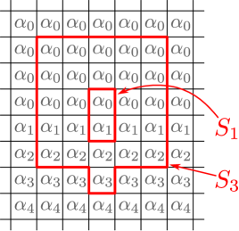
Figure 5.1. The surface $S\cong\Sigma(\lambda)$ from the proof of Proposition 5.4, where each square labelled by $\alpha_{n}$ denotes a copy of $\Sigma^{\circ}(\alpha_{n})=\mathbb{D}^{2}\smallsetminus[0,\omega^{\alpha}]$ (see Definition 5.1). There is an exhaustive filtration of $S$ by properly-embedded subsurfaces $S_{n}\cong\Sigma^{\circ}(\alpha_{n})$, described in the proof of Proposition 5.4; the boundaries of $S_{1}$ and $S_{3}$ are outlined in red.

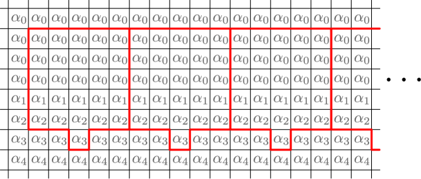
Figure 5.2. An extension of the inclusion $S_{n}\subset S$ (depicted in the case $n=3$) to a proper embedding $\mathrm{Str}(S_{n})\hookrightarrow S$, proving that $S_{n}$ is shiftable in $S$.

Proof of Proposition 5.4.

Let us construct a full-plane “grid surface” similarly to Definition 3.2, except that each square in the grid with coordinates $(i,j)\in\mathbb{Z}\times\mathbb{Z}$ is filled in with a copy of $\Sigma^{\circ}(\alpha_{\mathrm{max}(-j,0)})$. Equivalently, we begin with a copy of the half-plane grid surface $\mathrm{Gr}(\Sigma^{\circ}(\alpha_{0}))$, glue on a new row to the bottom of the grid filled with copies of $\Sigma^{\circ}(\alpha_{1})$, then another row filled with copies of $\Sigma^{\circ}(\alpha_{2})$, etc, until the whole grid is filled; see Figure 5.1. Let us denote this surface by $S$. Also, for each $n\geqslant 1$, we denote by $S_{n}\subset S$ the subsurface given by the union of all $(2n-1)^{2}$ pieces whose coordinates $(i,j)$ satisfy $\mathrm{max}(\lvert i\rvert,\lvert j\rvert)\leqslant n-1$, together with the piece whose coordinates are $(0,-n)$; see Figure 5.1. It follows from Lemma 1.10 that $S$ is homeomorphic to $\Sigma(\lambda)$ and each $S_{n}$ is homeomorphic to $\Sigma^{\circ}(\alpha_{n})$. Also, the $S_{n}$ (for $n\in\mathbb{N}$) form an exhaustive filtration of $S$ by properly-embedded subsurfaces.

Now let $\Sigma\subset\Sigma(\lambda)\cong S$ be any properly-embedded finite-type subsurface. It must be bounded away from the non-isolated end of $S$ “at infinity”, so it must be contained in $S_{n}$ for some $n\in\mathbb{N}$. To finish the proof, we just have to show that $S_{n}$ is shiftable in $S$: this is demonstrated pictorially in Figure 5.2. ∎

6. The punctured and unpunctured Cantor tree surfaces

In this section we prove Theorem D(1), dealing with the case when $S$ has genus zero and has either $0$ or $1$ punctures (isolated planar ends). This corresponds to exactly two possible homeomorphism types of surfaces: the sphere minus a Cantor set $\mathbb{S}^{2}\smallsetminus\mathcal{C}$ (the “Cantor tree surface”) and the plane minus a Cantor set $\mathbb{R}^{2}\smallsetminus\mathcal{C}$ (the “punctured Cantor tree surface”).

Both cases will follow almost immediately from the following result about the disc minus a Cantor set $\mathbb{D}^{2}\smallsetminus\mathcal{C}$ (the “one-holed Cantor tree surface”).

Theorem 6.1 ([PW, Theorem B]).

$\mathrm{Map}(\mathbb{D}^{2}\smallsetminus\mathcal{C})$ is acyclic, i.e. $H_{i}(\mathrm{Map}(\mathbb{D}^{2}\smallsetminus\mathcal{C}))=0$ for all $i>0$.

Proof of Theorem D(1).

Let $S$ be an infinite-type surface of genus zero with either no punctures (isolated ends) or exactly one puncture. By Remark 0.3 (the short exact sequence (0.1)), the subgroups $\mathrm{Map}_{c}(S)$ and $\mathrm{Map}_{f}(S)$ coincide whenever $S$ has at most one puncture. Thus we just have to consider an arbitrary compact subsurface $\Sigma\subset S$ and prove that the induced homomorphism $\mathrm{Map}(\Sigma)\to\mathrm{Map}(S)$ induces the zero map on homology in all positive degrees.

Since $S$ has genus zero, so does $\Sigma$, so it is homeomorphic to a sphere with $n$ holes for some $n\geqslant 1$. The complement $S\smallsetminus\Sigma$ thus has $n$ components, partitioning the end-space of $S$ into $n$ clopen subsets $E_{1},\ldots,E_{n}$. Since the end-space of $S$ is homeomorphic either to $\mathcal{C}$ or to $\mathcal{C}\sqcup\{*\}$, and all non-empty clopen subsets of $\mathcal{C}$ are homeomorphic to $\mathcal{C}$ again, we may assume (reordering if necessary) that $E_{1},\ldots,E_{n-1}$ are each homeomorphic to $\mathcal{C}$ or $\varnothing$ and $E_{n}$ is homeomorphic to $\mathcal{C}$ or $\varnothing$ or $\mathcal{C}\sqcup\{*\}$ or $\{*\}$. Denote by $\Sigma^{\prime}$ the subsurface of $S$ given by the union of $\Sigma$ together with the $n-1$ components of the complement $S\smallsetminus\Sigma$ corresponding to $E_{1},\ldots,E_{n-1}$. Since $\Sigma^{\prime}$ has genus zero, one (compact) boundary-component and has end-space homeomorphic to the disjoint union of some number (possibly zero) of copies of $\mathcal{C}$, it is homeomorphic either to $\mathbb{D}^{2}$ or to $\mathbb{D}^{2}\smallsetminus\mathcal{C}$. The homomorphism $\mathrm{Map}(\Sigma)\to\mathrm{Map}(S)$ factors through $\mathrm{Map}(\Sigma^{\prime})$, which is either the trivial group (if $\Sigma^{\prime}\cong\mathbb{D}^{2}$) or isomorphic to $\mathrm{Map}(\mathbb{D}^{2}\smallsetminus\mathcal{C})$, whose homology in all positive degrees vanishes by Theorem 6.1. ∎

Remark 6.2.

In contrast to our other vanishing results, Theorem D(1) holds for any coefficients, not only for coefficients in a field.

7. Non-trivial compactly-supported classes

In this section we prove all of our non-vanishing results – except for Theorem B(3) whose proof is deferred to §8 – for the images of $H_{*}(\mathrm{Map}_{c}(S))$ and $H_{*}(\mathrm{Map}_{f}(S))$ in $H_{*}(\mathrm{Map}(S))$. In §7.1 we prove Theorem C, dealing with the case when $S$ has non-zero but finite genus. In §7.2 we prove Theorem D(2), concerning Question II in the case when $S$ has finitely many but at least two punctures. In §7.3 we prove Theorem E, concerning the case when $S$ has genus zero and there is a finite, topologically-distinguished subset $A\subset{\mathrm{Ends}}(S)$ with $\lvert A\rvert\geqslant 4$. In the special case when $A$ is the set of punctures of $S$, this also proves Theorem D(3).

7.1. Finite, non-zero genus

In this subsection, we prove Theorem C, which we state slightly more precisely as the following:

Proposition 7.1.

Suppose that $1\leqslant g_{S}<\infty$. Then the integral homology $H_{*}(\mathrm{Map}(S))$ contains non-zero classes that are supported on a compact subsurface of $S$ homeomorphic to $\Sigma_{g_{S},1}$. More precisely, we may find such classes in degree $1$ when $g_{S}=1$ and in degree $2$ when $g_{S}\geqslant 2$.

In the proof, we will need the following calculations of low-degree homology groups of mapping class groups of closed, orientable surfaces.

Lemma 7.2.

We have $H_{1}(\mathrm{Map}(\Sigma_{1}))\cong\mathbb{Z}/12$ and

$$H_{2}(\mathrm{Map}(\Sigma_{g}))\cong\begin{cases}\mathbb{Z}/2&g=2\\ \mathbb{Z}\oplus\mathbb{Z}/2&g=3\\ \mathbb{Z}&g\geqslant 4.\end{cases}$$

Proof.

For the first statement, $\mathrm{Map}(\Sigma_{1})$ is isomorphic to $SL_{2}(\mathbb{Z})$, whose abelianisation is $\mathbb{Z}/12$. For the second statement, see [Kor02, Theorem 6.1 and the paragraph following it] for $g\geqslant 4$ and $g=2$. The case $g=3$ is not unambiguously settled in [Kor02]; instead, see [Sak12, Corollary 4.10]. See also [BCRR20, Lemma A.1] for these and many more related calculations. ∎

Proof of Proposition 7.1.

Since $S$ has finite genus $g_{S}$, all of its ends are planar and it is homeomorphic to $\Sigma_{g_{S}}\smallsetminus E$, where $E$ is the image of an embedding ${\mathrm{Ends}}(S)\hookrightarrow\Sigma_{g_{S}}$ of the end-space of $S$. Choose an embedded disc $D\subset\Sigma_{g_{S}}$ containing $E$ in its interior. There are homomorphisms

(7.1) $$\mathrm{Map}(\Sigma_{g_{S}}\smallsetminus\mathring{D})\longrightarrow\mathrm{Map}(\Sigma_{g_{S}}\smallsetminus E)\longrightarrow\mathrm{Map}(\Sigma_{g_{S}})$$

given respectively by extending homeomorphisms of $\Sigma_{g_{S}}\smallsetminus\mathring{D}$ (that are the identity on $\partial D$) by the identity on $D\smallsetminus E$ and extending homeomorphisms of $\Sigma_{g_{S}}\smallsetminus E$ to (its Freudenthal compactification) $\Sigma_{g_{S}}$ in the unique possible way (see [PW24, Appendix B] for why this determines a well-defined homomorphism of mapping class groups). The composition of the two homomorphisms (7.1) is the classical capping map $\mathrm{Map}(\Sigma_{g_{S}}\smallsetminus\mathring{D})\to\mathrm{Map}(\Sigma_{g_{S}})$ that extends homeomorphisms by the identity on $D$. This map induces a surjection on $H_{i}$ whenever $g_{S}\geqslant\frac{3}{2}(i-1)$ by part (3) of Theorem 4.3. In particular, it induces a surjection on $H_{1}$ whenever $g_{S}\geqslant 1$ and on $H_{2}$ whenever $g_{S}\geqslant 2$. It therefore suffices to check that $H_{1}(\mathrm{Map}(\Sigma_{1}))\neq 0$ and that $H_{2}(\mathrm{Map}(\Sigma_{g_{S}}))\neq 0$ when $g_{S}\geqslant 2$. This follows from Lemma 7.2. ∎

7.2. Finitely many punctures but at least two

In this subsection, we prove Theorem D(2). In fact, this part of Theorem D does not require the assumption that $g_{S}=0$, so we may strengthen it to:

Proposition 7.3.

Suppose that $2\leqslant p_{S}<\infty$. Then $H_{*}(\mathrm{Map}(S))$ contains a non-trivial class that is supported on a properly-embedded finite-type subsurface of $S$.

Proof.

Since $p=p_{S}$ is finite, there is a properly-embedded subsurface of $S$ homeomorphic to the punctured disc $\mathbb{D}^{2}\smallsetminus P$, where $P$ is a finite set of size $p$ in the interior of $\mathbb{D}^{2}$. This induces an extension map $B_{p}=\mathrm{Map}(\mathbb{D}^{2}\smallsetminus P)\to\mathrm{Map}(S)$, where $B_{p}$ denotes the braid group on $p$ strands. For any homeomorphism of $S$, its induced action on the end-space ${\mathrm{Ends}}(S)$ must send the subset of punctures onto itself, so there is a well-defined map $\mathrm{Map}(S)\to\mathfrak{S}_{p}$ recording this permutation. The composition $B_{p}\to\mathfrak{S}_{p}$ records the permutation induced by a braid, and is surjective. Since abelianisation $(-)^{ab}=H_{1}(-)$ is a right-exact functor, the composition of the induced maps $H_{1}(B_{p})\to H_{1}(\mathrm{Map}(S))\to H_{1}(\mathfrak{S}_{p})$ is also surjective. Since $H_{1}(\mathfrak{S}_{p})\cong\mathbb{Z}/2$ (here we are using the assumption that $p\geqslant 2$), we may choose a lift $\alpha\in H_{1}(B_{p})$ of the non-trivial element of $H_{1}(\mathfrak{S}_{p})$. The image of $\alpha$ in $H_{1}(\mathrm{Map}(S))$ is then a non-trivial class supported on a properly-embedded finite-type subsurface. ∎

The above proof does not work when $p=p_{S}=1$, since $H_{1}(\mathfrak{S}_{p})$ is trivial in this case. Indeed, in this case, the answer to Question II depends also on the genus of $S$. If $g_{S}=0$ then $S$ must be homeomorphic to $\mathbb{R}^{2}\smallsetminus\mathcal{C}$ and the answer is given in §6 above. The case when $0<g_{S}<\infty$ is covered by Proposition 7.1 above. The case when $g_{S}=\infty$ is dealt with in §8 below.

7.3. Genus zero with a finite, topologically-distinguished set of ends

We next prove Theorem E (which in particular implies Theorem D(3)). Recall from Definition 0.10 the notion of a topologically distinguished subset. The following is a refinement of Theorem E.

Proposition 7.4.

Suppose that $S$ has genus zero and that ${\mathrm{Ends}}(S)$ has a finite, topologically distinguished subset of size $n\geqslant 2$. Set $k=n-1$ if $n$ is even and $k=\frac{1}{2}(n-1)$ if $n$ is odd. Then there is a commutative diagram

(7.2)

where the left-hand vertical map is induced by the inclusion $\mathrm{Map}_{c}(S)\subset\mathrm{Map}(S)$, the right-hand vertical map is multiplication by $2$ and the top horizontal map is surjective. In particular, if $n\geqslant 4$, there are non-trivial classes in $H_{1}(\mathrm{Map}(S))$ that are supported on a compact subsurface.

Remark 7.5.

We do not require the finite, topologically-distinguished subset of ${\mathrm{Ends}}(S)$ in Proposition 7.4 to be homogeneous; for example, it may consist of $n$ points that are each (individually) topologically-distinguished. The bottom horizontal map of (7.2) is surjective if and only if this is not the case, i.e. two of the points of the (chosen) topologically-distinguished subset are similar, i.e. have homeomorphic open neighbourhoods.

Proof of Proposition 7.4.

We first note that the second statement follows from the first: when $n\geqslant 4$ we have $k\geqslant 2$, so the element $2\in\mathbb{Z}/2k$ is non-trivial and pulls back through $H_{1}(\mathrm{Map}(S))$ to $H_{1}(\mathrm{Map}_{c}(S))$. Hence we just have to prove the first statement.

Denote by $A\subset{\mathrm{Ends}}(S)$ a topologically distinguished subset of size $n$. Since ${\mathrm{Ends}}(S)$ is Hausdorff and zero-dimensional, we may partition it into clopen subsets $E_{1},\ldots,E_{n}$ such that each $E_{i}$ contains exactly one point of $A$. Let $S_{i}=\mathbb{D}^{2}\smallsetminus E_{i}$ for $i\in\{1,\ldots,n\}$ and denote by $\Sigma_{0,n}$ the compact, connected genus-$0$ surface with $n$ boundary components. Gluing $S_{1},\ldots,S_{n}$ into the $n$ holes of $\Sigma_{0,n}$ we obtain $\mathbb{S}^{2}\smallsetminus{\mathrm{Ends}}(S)$, which is homeomorphic to $S$. There is therefore an extension homomorphism $\mathrm{Map}(\Sigma_{0,n})\to\mathrm{Map}_{c}(S)$ given by extending homeomorphisms by the identity on each $S_{i}$. On the other hand, since $A\subset{\mathrm{Ends}}(S)$ is a topologically distinguished subset, we have a homomorphism $\mathrm{Map}(S)\to\mathrm{Map}(\mathbb{S}^{2}\smallsetminus A)$ given by filling in all ends of $S$ except $A$. Next, there is a central extension [FM11, §9.1.4]

$$1\to\mathbb{Z}/2\longrightarrow B_{n}(\mathbb{S}^{2})\longrightarrow\mathrm{Map}(\mathbb{S}^{2}\smallsetminus A)\to 1,$$

where the generator of the kernel is sent to a full twist in the spherical braid group $B_{n}(\mathbb{S}^{2})$. This is sent to $n(n-1)$ in $B_{n}(\mathbb{S}^{2})^{ab}\cong\mathbb{Z}/(2n-2)$, which is $0$ if $n$ is even and $n-1$ if $n$ is odd. Let us consider the quotient of $B_{n}(\mathbb{S}^{2})$ onto its abelianisation $\mathbb{Z}/(2n-2)$ when $n$ is even and the further quotient onto $\mathbb{Z}/(n-1)$ when $n$ is odd; we may write this uniformly as the quotient $B_{n}(\mathbb{S}^{2})\twoheadrightarrow\mathbb{Z}/2k$ where $k=n-1$ if $n$ is even and $k=\frac{1}{2}(n-1)$ if $n$ is odd. By construction, the kernel $\mathbb{Z}/2\subset B_{n}(\mathbb{S}^{2})$ of the central extension above is sent to zero in this quotient, so it factors through a quotient $\mathrm{Map}(\mathbb{S}^{2}\smallsetminus A)\twoheadrightarrow\mathbb{Z}/2k$. Putting everything together, we have maps

(7.3) $$\mathrm{Map}(\Sigma_{0,n})\longrightarrow\mathrm{Map}_{c}(S)\subset\mathrm{Map}(S)\longrightarrow\mathrm{Map}(\mathbb{S}^{2}\smallsetminus A)\longrightarrow\mathbb{Z}/2k.$$

The composition $\mathrm{Map}_{c}(S)\to\mathbb{Z}/2k$ is not surjective; instead, its image is the cyclic subgroup of order $k$ generated by $2\in\mathbb{Z}/2k$. To see this, first note that a pre-image of the element $2\in\mathbb{Z}/2k$ in $\mathrm{Map}(\Sigma_{0,n})$ (which may then be extended to $\mathrm{Map}_{c}(S)$) is given by a homeomorphism that “pushes” one boundary component in a full loop around another boundary component. This implies that the image contains the cyclic subgroup generated by $2$. On the other hand, it cannot be larger than this, since every element of $\mathrm{Map}_{c}(S)$ has compact support and hence its induced permutation of $A$ is trivial, which is an even permutation. Thus we have the following commutative diagram:

Taking abelianisations, we obtain the desired commutative diagram (7.2). ∎

8. Classes detected by wreath products of the circle group

In this section we prove Theorem B(3), which we restate in a stronger form as Proposition 8.1 below. We want to consider surfaces of infinite genus with finitely many (and at least one) punctures. However, it will be more convenient to think of the punctures as marked points, so we fix a surface $S$ of infinite genus and no punctures, together with a non-empty, finite subset $P\subset S$, and we shall be interested in Question II for the surface $S\smallsetminus P$. In other words, we are interested in the image of the map

(8.1) $$H_{*}(\mathrm{Map}_{f}(S\smallsetminus P))\longrightarrow H_{*}(\mathrm{Map}(S\smallsetminus P))$$

induced by the inclusion $\mathrm{Map}_{f}(S\smallsetminus P)\subset\mathrm{Map}(S\smallsetminus P)$. Question II asks whether its image is non-zero for some positive degree $*>0$. In fact we may prove that it is non-zero in every even degree:

Proposition 8.1.

Let $S$ be a connected, orientable surface of infinite genus with no punctures and $P\subset S$ a non-empty, finite subset. Then the image of the map (8.1) contains a $\mathbb{Z}$ summand in every even degree; in particular it is non-zero.

A key ingredient of the proof is a construction due to Bödigheimer and Tillmann [BT01].

Notation 8.2.

For a surface $S$ (possibly with boundary) and finite subset $P\subset\mathring{S}$ of its interior, denote by $\mathrm{Diff}(S,P)$ the topological group of diffeomorphisms of $S$ that fix $P$ setwise and $\partial S$ pointwise, equipped with the weak (“smooth compact-open”) topology [Hir76, §2.1].

Definition 8.3 ([BT01, §3]).

For a surface $S$ (possibly with boundary) and finite subset $P\subset\mathring{S}$ of size $p=\lvert P\rvert$, let

(8.2) $$\tau\colon\mathrm{Diff}(S,P)\longrightarrow\mathbb{S}^{1}\wr\mathfrak{S}_{p}=(\mathbb{S}^{1})^{p}\rtimes\mathfrak{S}_{p}$$

be the continuous homomorphism defined as follows. Choose a bijection $i\mapsto x_{i}\colon\{1,\ldots,p\}\to P$ and choose a tangent vector $v_{i}\in T_{x_{i}}S$ for each $i\in\{1,\ldots,p\}$. For a diffeomorphism $\varphi$, the map $\tau$ records the induced permutation $\sigma(\varphi)$ of $\{1,\ldots,p\}$ under the chosen bijection and the angle $\theta_{i}(\varphi)$ between $D\varphi(v_{i})$ and $v_{\sigma(i)}$ for each $i\in\{1,\ldots,p\}$, where $D\varphi$ denotes the derivative of $\varphi$.

Notation 8.4.

Write $BG$ for the classifying space of a topological group $G$. When $G$ is discrete the homology of $BG$ agrees with the group homology of $G$, so we shall write $H_{*}(BG)=H_{*}(G)$.

Construction 8.5.

Let $S$ be a surface with no punctures and $P\subset S$ a finite subset of size $p=\lvert P\rvert$. We shall use (8.2) to construct a map

(8.3) $$B\mathrm{Map}_{f}(S\smallsetminus P)\longrightarrow B(\mathbb{S}^{1}\wr\mathfrak{S}_{p}).$$

Let $\Sigma\subset S$ be a compact subsurface containing $P$ in its interior. We then have maps

(8.4) $$\mathrm{Map}(\Sigma\smallsetminus P)\cong\pi_{0}(\mathrm{Diff}(\Sigma,P))\twoheadleftarrow\joinrel\relbar\mathrm{Diff}(\Sigma,P)\longrightarrow\mathbb{S}^{1}\wr\mathfrak{S}_{p},$$

where the right-hand map is (8.2). These are all compatible with the maps induced by inclusions of subsurfaces, so there are induced maps of colimits

(8.5) $$\underset{\Sigma}{\mathrm{colim}}(\mathrm{Map}(\Sigma\smallsetminus P))\cong\underset{\Sigma}{\mathrm{colim}}(\pi_{0}(\mathrm{Diff}(\Sigma,P)))\twoheadleftarrow\joinrel\relbar\underset{\Sigma}{\mathrm{colim}}(\mathrm{Diff}(\Sigma,P))\longrightarrow\mathbb{S}^{1}\wr\mathfrak{S}_{p},$$

where each colimit is taken over the poset of all compact subsurfaces $\Sigma\subset S$ with $P\subset\mathring{\Sigma}$. Since $S$ has no punctures, the left-hand group in (8.5) may be identified with $\mathrm{Map}_{f}(S\smallsetminus P)$.

The middle map in (8.4) is a weak homotopy equivalence by [EE69, ES70] and hence so is the middle map in (8.5). Taking classifying spaces and inverting this map, we obtain the desired map (8.3).

The key ingredient to prove Proposition 8.1 is the following corollary of the main result of [BT01].

Theorem 8.6.

If $S$ is a connected, orientable surface of infinite genus with no punctures and $P\subset S$ is a finite subset, then the map

(8.6) $$H_{*}(\mathrm{Map}_{f}(S\smallsetminus P))\longrightarrow H_{*}(B(\mathbb{S}^{1}\wr\mathfrak{S}_{p}))$$

induced on homology by (8.3) admits a section.

Proof.

In fact, [BT01] makes a stronger statement. Let us write $(-)^{+}$ for the Quillen plus-construction of a topological space (see [BT01, §2] for a brief summary of some key properties of the plus-construction and for example [Ber82] for further details). According to [BT01, Theorem 1.1 (2)], the space $B\mathrm{Map}_{f}(S\smallsetminus P)^{+}$ splits, up to homotopy equivalence, as the product of $B\Gamma_{\infty}^{+}$ and $B(\mathbb{S}^{1}\wr\mathfrak{S}_{p})^{+}$, where $\Gamma_{\infty}$ denotes the colimit of $\mathrm{Map}(\Sigma_{g,1})$ as $g\to\infty$, and (the plus-construction of) the map (8.3) is the projection onto the second factor of this decomposition. It therefore admits a section up to homotopy, so the result follows upon taking homology since $(-)^{+}$ does not change the homology of a space. In [BT01], this result is stated for the particular surface $S=\mathrm{colim}_{g\to\infty}(\Sigma_{g,1})$, but the homology $H_{*}(\mathrm{Map}_{f}(S\smallsetminus P))$ is the same for any surface $S$ satisfying the hypotheses of the theorem, by [Har85]; alternatively, the proof of [BT01] goes through for any such surface $S$, by taking the colimit of an appropriate diagram of stabilisation maps, corresponding to a filtration of $S$ by compact subsurfaces. ∎

To complete the proof of Proposition 8.1 we need two further ingredients.

Lemma 8.7.

The homology $H_{*}(B(\mathbb{S}^{1}\wr\mathfrak{S}_{p}))$ contains a $\mathbb{Z}$ summand in every even degree.

Proof.

When $p=1$ this is $H_{*}(B\mathbb{S}^{1})=H_{*}(\mathbb{C}\mathbb{P}^{\infty})$, which is $\mathbb{Z}$ in every even degree and $0$ in odd degrees. For any topological abelian group $A$, the wreath product $A\wr\mathfrak{S}_{p}$ retracts onto $A$ via the maps $A\to A\wr\mathfrak{S}_{p}$ and $A\wr\mathfrak{S}_{p}\to A$ defined by $a\mapsto(a,0,\ldots,0;\mathrm{id})$ and $(a_{1},\ldots,a_{p};\sigma)\mapsto a_{1}+\cdots+a_{p}$. It then follows that $H_{*}(B\mathbb{S}^{1})=H_{*}(\mathbb{C}\mathbb{P}^{\infty})$ is a summand in $H_{*}(B(\mathbb{S}^{1}\wr\mathfrak{S}_{p}))$. ∎

Proposition 8.8.

If $S$ is a connected, orientable surface with no punctures and $P\subset S$ is a finite subset, then the map (8.3) extends along $B(\mathrm{incl})\colon B\mathrm{Map}_{f}(S\smallsetminus P)\to B\mathrm{Map}(S\smallsetminus P)$.

Before proving Proposition 8.8, we first show how it – together with Theorem 8.6 and Lemma 8.7 – implies Proposition 8.1 (and hence Theorem B(3)).

Proof of Proposition 8.1.

By Theorem 8.6 and Proposition 8.8, we have maps

$$H_{*}(B(\mathbb{S}^{1}\wr\mathfrak{S}_{p}))\longrightarrow H_{*}(\mathrm{Map}_{f}(S\smallsetminus P))\longrightarrow H_{*}(\mathrm{Map}(S\smallsetminus P))\longrightarrow H_{*}(B(\mathbb{S}^{1}\wr\mathfrak{S}_{p}))$$

whose composition is the identity. It follows that $H_{*}(B(\mathbb{S}^{1}\wr\mathfrak{S}_{p}))$, which contains a $\mathbb{Z}$ summand in every even degree by Lemma 8.7, is a direct summand in the image of $H_{*}(\mathrm{Map}_{f}(S\smallsetminus P))\to H_{*}(\mathrm{Map}(S\smallsetminus P))$. ∎

$$\begin{split}\leavevmode\hbox to415.72pt{\vbox to278.38pt{\text{[drawing]}}}\end{split} \mathbb{S}^{1}\wr\mathfrak{S}_{p} \mathrm{Diff}(\Sigma,P) \mathrm{Diff}(S,P) \mathrm{Homeo}(\Sigma,P) \mathrm{Homeo}(S,P) \mathrm{Homeo}(\Sigma\smallsetminus P) \mathrm{Homeo}(S\smallsetminus P) \pi_{0}(\mathrm{Diff}(\Sigma,P)) \pi_{0}(\mathrm{Diff}(S,P)) \pi_{0}(\mathrm{Homeo}(\Sigma,P)) \pi_{0}(\mathrm{Homeo}(S,P)) \pi_{0}(\mathrm{Homeo}(\Sigma\smallsetminus P)) \pi_{0}(\mathrm{Homeo}(S\smallsetminus P)) \mathrm{Map}(\Sigma\smallsetminus P) \mathrm{Map}(S\smallsetminus P)^{\delta} \mathrm{Map}(S\smallsetminus P) \simeq \cong \simeq \cong \cong \cong \cong \cong \simeq = = \mathbb{S}^{1}\wr\mathfrak{S}_{p} \mathrm{Diff}(\Sigma,P) \mathrm{Diff}(S,P) \mathrm{Homeo}(\Sigma,P) \mathrm{Homeo}(S,P) \mathrm{Homeo}(\Sigma\smallsetminus P) \mathrm{Homeo}(S\smallsetminus P) \pi_{0}(\mathrm{Diff}(\Sigma,P)) \pi_{0}(\mathrm{Diff}(S,P)) \pi_{0}(\mathrm{Homeo}(\Sigma,P)) \pi_{0}(\mathrm{Homeo}(S,P)) \pi_{0}(\mathrm{Homeo}(\Sigma\smallsetminus P)) \pi_{0}(\mathrm{Homeo}(S\smallsetminus P)) \mathrm{Map}(\Sigma\smallsetminus P) \mathrm{Map}(S\smallsetminus P)^{\delta} \mathrm{Map}(S\smallsetminus P) \simeq \cong \simeq \cong \cong \cong \cong \cong \simeq = =$$

Figure 8.1. The diagram used to construct the extension of (8.3) to $B\mathrm{Map}(S\smallsetminus P)$ in the proof of Proposition 8.8. The surface $S$ is connected, orientable and has no punctures (in other words, all of its ends are either non-planar or non-isolated), $P\subset S$ is a finite subset and $\Sigma\subset S$ is a compact subsurface containing $P$ in its interior.

Proof of Proposition 8.8.

At the level of diffeomorphism groups, the construction clearly extends to a well-defined continuous homomorphism $\mathrm{Diff}(S,P)\to\mathbb{S}^{1}\wr\mathfrak{S}_{p}$. Indeed, Definition 8.3 does not make any compactness assumptions. The only subtlety lies in descending this homomorphism to the mapping class group.

We first recall the construction of the map (8.3) in more detail. In the diagram in Figure 8.1, $S$ and $P\subset S$ are as in Proposition 8.8 and $\Sigma\subset S$ is any compact subsurface containing $P$ in its interior. The natural map from the diffeomorphism group to the homeomorphism group of any smooth surface is a weak equivalence (in particular an isomorphism on $\pi_{0}$) and the restriction map $\mathrm{Homeo}(S,P)\to\mathrm{Homeo}(S\smallsetminus P)$ is an isomorphism of topological groups when $S$ has no punctures, since one may define an inverse by extending homeomorphisms uniquely to the Freudenthal compactification of $S\smallsetminus P$ and then discarding all ends that are not punctures (these are preserved by any homeomorphism). Thus all of the vertical maps in Figure 8.1 are either weak equivalences or isomorphisms. The horizontal map across the top is the homomorphism (8.2) of Definition 8.3. To identify its domain with $\mathrm{Map}(\Sigma\smallsetminus P)=\pi_{0}(\mathrm{Homeo}(\Sigma\smallsetminus P))$, we need to know that the diagonal maps on the left-hand side are also weak equivalences, which follows either from [EE69, ES70] at the level of diffeomorphism groups or from [Ham66] at the level of homeomorphism groups. Taking the colimit over all $\Sigma$, and then taking classifying spaces, we obtain the map (8.3).

To see that (8.3) extends to $B\mathrm{Map}(S\smallsetminus P)$, we need to know that the diagonal maps on the right-hand side are also weak equivalences. This follows from the main result of [Yag00], which extends [Ham66] to non-compact surfaces, proving that $\mathrm{Homeo}(S\smallsetminus P)$ has contractible components (and thus contractible path-components), so the projection $\mathrm{Homeo}(S\smallsetminus P)\to\pi_{0}(\mathrm{Homeo}(S\smallsetminus P))$ is a weak equivalence. There is a small additional subtlety: for this projection map to make sense, one has to equip $\mathrm{Map}(S\smallsetminus P)=\pi_{0}(\mathrm{Homeo}(S\smallsetminus P))$ with the quotient topology induced by the compact-open topology, whereas we are interested in it as an abstract group, equivalently equipped with the discrete topology. Let us temporarily take the convention that $\mathrm{Map}(S\smallsetminus P)$ denotes the mapping class group with the quotient topology and $\mathrm{Map}(S\smallsetminus P)^{\delta}$ denotes the same group with the discrete topology. Since $\mathrm{Map}(S\smallsetminus P)$ is totally disconnected (in fact it is homeomorphic to the Baire space $\mathbb{N}^{\mathbb{N}}$ [AV20, Thm 4.2]), the map $\mathrm{Map}(S\smallsetminus P)^{\delta}\to\mathrm{Map}(S\smallsetminus P)$ given by the identity of the underlying groups is a weak equivalence. Together, this implies that the map (8.3) extends from $B\mathrm{Map}_{f}(S\smallsetminus P)=B\underset{\Sigma}{\mathrm{colim}}(\mathrm{Map}(\Sigma\smallsetminus P))$ to $B\mathrm{Map}(S\smallsetminus P)^{\delta}$. ∎

References

- [APV20] Javier Aramayona, Priyam Patel, and Nicholas G. Vlamis. The first integral cohomology of pure mapping class groups. Int. Math. Res. Not. IMRN, 2020(22):8973–8996, 2020.
- [AV20] Javier Aramayona and Nicholas G. Vlamis. Big mapping class groups: an overview. In Ken’ichi Ohshika and Athanase Papadopoulos, editors, In the Tradition of Thurston: Geometry and Topology, pages 459–496. Springer, 2020.
- [BCRR20] Dave Benson, Caterina Campagnolo, Andrew Ranicki, and Carmen Rovi. Signature cocycles on the mapping class group and symplectic groups. J. Pure Appl. Algebra, 224(11):106400, 49, 2020.
- [Ber82] A. Jon Berrick. An approach to algebraic -theory, volume 56 of Research Notes in Mathematics. Pitman (Advanced Publishing Program), Boston, Mass.-London, 1982.
- [Ber02] A. J. Berrick. A topologist’s view of perfect and acyclic groups. In Invitations to geometry and topology, volume 7 of Oxf. Grad. Texts Math., pages 1–28. Oxford Univ. Press, Oxford, 2002.
- [BM79] Edward M. Brown and Robert Messer. The classification of two-dimensional manifolds. Trans. Amer. Math. Soc., 255:377–402, 1979.
- [Bol12] Søren K. Boldsen. Improved homological stability for the mapping class group with integral or twisted coefficients. Math. Z., 270(1-2):297–329, 2012.
- [BT01] Carl-Friedrich Bödigheimer and Ulrike Tillmann. Stripping and splitting decorated mapping class groups. In Cohomological methods in homotopy theory (Bellaterra, 1998), volume 196 of Progr. Math., pages 47–57. Birkhäuser, Basel, 2001.
- [Dom22] George Domat. Big pure mapping class groups are never perfect. Math. Res. Lett., 29(3):691–726, 2022. Appendix with Ryan Dickmann.
- [EE69] Clifford J. Earle and James Eells. A fibre bundle description of Teichmüller theory. J. Differential Geometry, 3:19–43, 1969.
- [ES70] C. J. Earle and A. Schatz. Teichmüller theory for surfaces with boundary. J. Differential Geometry, 4:169–185, 1970.
- [FM11] Benson Farb and Dan Margalit. A primer on mapping class groups. Princeton, NJ: Princeton University Press, 2011.
- [Ham66] Mary-Elizabeth Hamstrom. Homotopy groups of the space of homeomorphisms on a -manifold. Illinois J. Math., 10:563–573, 1966.
- [Har85] John L. Harer. Stability of the homology of the mapping class groups of orientable surfaces. Ann. of Math. (2), 121(2):215–249, 1985.
- [Hir76] Morris W. Hirsch. Differential topology, volume No. 33 of Graduate Texts in Mathematics. Springer-Verlag, New York-Heidelberg, 1976.
- [HW10] Allen Hatcher and Nathalie Wahl. Stabilization for mapping class groups of 3-manifolds. Duke Math. J., 155(2):205–269, 2010.
- [Iva93] Nikolai V. Ivanov. On the homology stability for Teichmüller modular groups: closed surfaces and twisted coefficients. In Mapping class groups and moduli spaces of Riemann surfaces (Göttingen, 1991/Seattle, WA, 1991), volume 150 of Contemp. Math., pages 149–194. Amer. Math. Soc., Providence, RI, 1993.
- [Jec03] Thomas Jech. Set theory. Springer Monographs in Mathematics. Springer-Verlag, Berlin, millennium edition, 2003.
- [Kor02] Mustafa Korkmaz. Low-dimensional homology groups of mapping class groups: a survey. Turkish J. Math., 26(1):101–114, 2002.
- [KS77] Robion C. Kirby and Laurence C. Siebenmann. Foundational essays on topological manifolds, smoothings, and triangulations. Annals of Mathematics Studies, No. 88. Princeton University Press, Princeton, N.J.; University of Tokyo Press, Tokyo, 1977. With notes by John Milnor and Michael Atiyah.
- [Mat71] John N. Mather. The vanishing of the homology of certain groups of homeomorphisms. Topology, 10:297–298, 1971.
- [MS20] Stefan Mazurkiewicz and Wacław Sierpiński. Contribution à la topologie des ensembles dénombrables. Fundam. Math., 1:17–27, 1920.
- [MT] Justin Malestein and Jing Tao. Self-similar surfaces: involutions and perfection. ArXiv:2106.03681.
- [Mum83] David Mumford. Towards an enumerative geometry of the moduli space of curves. In Arithmetic and geometry, Vol. II, volume 36 of Progr. Math., pages 271–328. Birkhäuser Boston, Boston, MA, 1983.
- [MW07] Ib Madsen and Michael Weiss. The stable moduli space of Riemann surfaces: Mumford’s conjecture. Ann. of Math. (2), 165(3):843–941, 2007.
- [PW] Martin Palmer and Xiaolei Wu. On the homology of big mapping class groups. ArXiv:2211.07470.
- [PW24] Martin Palmer and Xiaolei Wu. Big mapping class groups with uncountable integral homology. Doc. Math., 29(1):159–189, 2024.
- [Ric63] Ian Richards. On the classification of noncompact surfaces. Trans. Amer. Math. Soc., 106:259–269, 1963.
- [RW16] Oscar Randal-Williams. Resolutions of moduli spaces and homological stability. J. Eur. Math. Soc. (JEMS), 18(1):1–81, 2016.
- [Sak12] Takuya Sakasai. Lagrangian mapping class groups from a group homological point of view. Algebr. Geom. Topol., 12(1):267–291, 2012.
- [Sie58] Wacław Sierpiński. Cardinal and ordinal numbers, volume Tom 34 of Polska Akademia Nauk. Monografie Matematyczne. Państwowe Wydawnictwo Naukowe, Warsaw, 1958.
- [vK23] B. von Kerékjártó. Vorlesungen über Topologie. I.: Flächentopologie., volume 8 of Grundlehren Math. Wiss. Springer, Cham, 1923.
- [Wah13] Nathalie Wahl. Homological stability for mapping class groups of surfaces. In Handbook of moduli. Vol. III, volume 26 of Adv. Lect. Math. (ALM), pages 547–583. Int. Press, Somerville, MA, 2013.
- [Yag00] Tatsuhiko Yagasaki. Homotopy types of homeomorphism groups of noncompact -manifolds. Topology Appl., 108(2):123–136, 2000.