On the Influence of Data Resampling for Deep Learning-Based Log Anomaly Detection: Insights and Recommendations

Abstract

Numerous Deep Learning (DL)-based approaches have garnered considerable attention in the field of software Log Anomaly Detection (LAD). However, a practical challenge persists: the prevalent issue of class imbalance in the public data commonly used to train the DL models. This imbalance is characterized by a substantial disparity in the number of abnormal log sequences compared to normal ones, for example, anomalies represent less than 1% of one of the most popular datasets, namely the Thunderbird dataset. Previous research has indicated that existing DLLAD approaches may exhibit unsatisfactory performance, particularly when confronted with datasets featuring severe class imbalances. Mitigating class imbalance through data resampling has proven effective for other software engineering tasks, however, it has been unexplored for LAD thus far. This study aims to fill this gap by providing an in-depth analysis of the impact of diverse data resampling methods on existing DLLAD approaches from two distinct perspectives. Firstly, we assess the performance of these DLLAD approaches across three datasets, and explore the impact of resampling ratios of normal to abnormal data on ten data resampling methods. Secondly, we evaluate the effectiveness of the data resampling methods when utilizing optimal resampling ratios of normal to abnormal data. Our findings indicate that oversampling methods generally outperform undersampling and hybrid sampling methods. Data resampling on raw data yields superior results compared to data resampling in the feature space. In most cases, certain undersampling and hybrid methods (e.g., SMOTEENN and InstanceHardnessThreshold) show limited effectiveness. Additionally, by exploring the resampling ratio of normal to abnormal data, we suggest generating more data for minority classes through oversampling while removing less data from majority classes through undersampling. In conclusion, our study provides valuable insights into the intricate relationship between data resampling methods and DLLAD. By addressing the challenge of class imbalance, researchers and practitioners can enhance the model performance in DLLAD.

I Introduction

Software-intensive systems, which cater to a wide user base [1], are susceptible to minor issues that can lead to adverse consequences such as data corruption and performance degradation [2]. In this context, logs play a crucial role in system maintenance [3, 4, 5, 6], as they capture essential runtime information required for troubleshooting and performance monitoring [7]. Consequently, there is a considerable interest in utilizing logs for anomaly detection. Recently, many Deep Learning-based Log Anomaly Detection (DLLAD) approaches [8, 9, 10, 11, 2, 12, 13] have been proposed to automatically identify system anomalies, showing promising results.

In real-world scenarios in DLLAD, the proportion of normal data significantly outweighs that of abnormal data. For instance, consider the Thunderbird dataset in Table I, one of the commonly used public datasets where logs are grouped into log sequences (with 20, 50, or 100 logs constituting a sequence) for data analysis. In this dataset, anomalies only account for 0.16%–0.35% of the total, highlighting the serious imbalance in the data distribution. Le et al. [1] have revealed that DLLAD models trained on highly imbalanced datasets exhibit low precision or recall values. Low recall leads to missed anomalies, leaving potential threats undetected, while low precision generates numerous false alarms, causing alert fatigue and resource wastage on normal logs [12, 1, 13].

Nonetheless, the issue of class imbalance in DLLAD has remained unaddressed. Data resampling offers an alternative by generating abnormal data or removing normal data, thereby enabling the model to learn from a more balanced representation of both classes. In this study, we aim to assess the impact of data resampling on the performance of existing DLLAD approaches and explore the optimal ratio of normal to abnormal data for data resampling. To achieve these goals, we conduct an extensive empirical study by employing three oversampling methods (Random OverSampling (ROS), SMOTE [14], and ADASYN [15]), three undersampling methods (Random UnderSampling (RUS), NearMiss [16], and InstanceHardnessThreshold [17]), and two hybrid sampling methods (SMOTEENN [18] and SMOTETomek [18]) to DLLAD approaches (CNN [9], LogRobust [10], NeuralLog [2]) across three publicly available datasets. We compare the results with DLLAD approaches with NoSampling (using the original dataset). Furthermore, the data resampling methods can also be categorized into resampling on raw data and resampling in the feature space. It is important to note that many data resampling methods are designed for application only within the feature space, as they rely on distance computations. Simpler methods, like ROS and RUS, can be applied to both raw data (duplicating/removing log sequences with identical texts) and feature space (duplicating/removing sequences with the same embedding vectors). We structure our study with the following research questions:

• RQ1: Do the existing DLLAD approaches perform well enough with varying degrees of class imbalance?

  We first evaluate the performance of existing DLLAD approaches across datasets with diverse levels of class imbalance. Findings: The performance of DLLAD approaches is significantly influenced by the degree of class imbalance, with their effectiveness notably decreasing when faced with severe data imbalance.

• RQ2: How does the resampling ratio of normal to abnormal data affect the ability of data resampling?

  We explore how varying the resampling ratio of normal to abnormal data impacts the results by using quarter-based multipliers of the original ratio of normal to abnormal log sequences. Findings: The effectiveness of oversampling methods on DLLAD approaches is maximized when generating more abnormal log sequences. Conversely, removing fewer normal log sequences enhances the effectiveness of undersampling methods on DLLAD approaches. When DLLAD approaches already perform well on specific datasets without applying data resampling methods, they become less sensitive to the choice of the resampling ratio.

• RQ3: Does data resampling improve the effectiveness of existing DLLAD approaches?

  We assess the effectiveness of data resampling on DLLAD approaches utilizing an optimal resampling ratio (obtained from RQ2) of normal to abnormal data. Findings: Overall, oversampling methods demonstrate superior performance compared to undersampling and hybrid sampling methods. Remarkably, the straightforward methods applied directly to raw data outperform other methods applied within the feature space. Surprisingly, in many scenarios, some more advanced undersampling methods (i.e., NearMiss and InstanceHardnessThreshold), and even a hybrid sampling method SMOTEENN aimed at mitigating data imbalance, fail to effectively enhance the performance of DLLAD approaches.

In summary, our study makes the following two contributions.

• To the best of our knowledge, we undertake the first extensive study aimed at systematically assessing the impact of data resampling methods on model performance in DLLAD. Our study encompasses a total of 4,185 experiments, wherein we employ ten data resampling methods to existing DLLAD approaches and provide a comprehensive evaluation and statistical analysis across three publicly available benchmark datasets.

• Based on the empirical results, we conclude the findings and provide recommendations to researchers and software developers in the field of anomaly detection. We recommend that practitioners 1) prefer oversampling with generating more abnormal log sequences over undersampling and hybrid sampling and 2) prioritize data resampling on raw data over data resampling within the feature space. However, we do not recommend practitioners use SMOTEENN for datasets with extremely high class imbalance.

II Background

II-A Overview of DLLAD Models

The typical workflow of DLLAD approaches (shown in Figure 1) consists of four phases: 1) log parsing, 2) log grouping, 3) log embedding, and 4) model training and prediction.

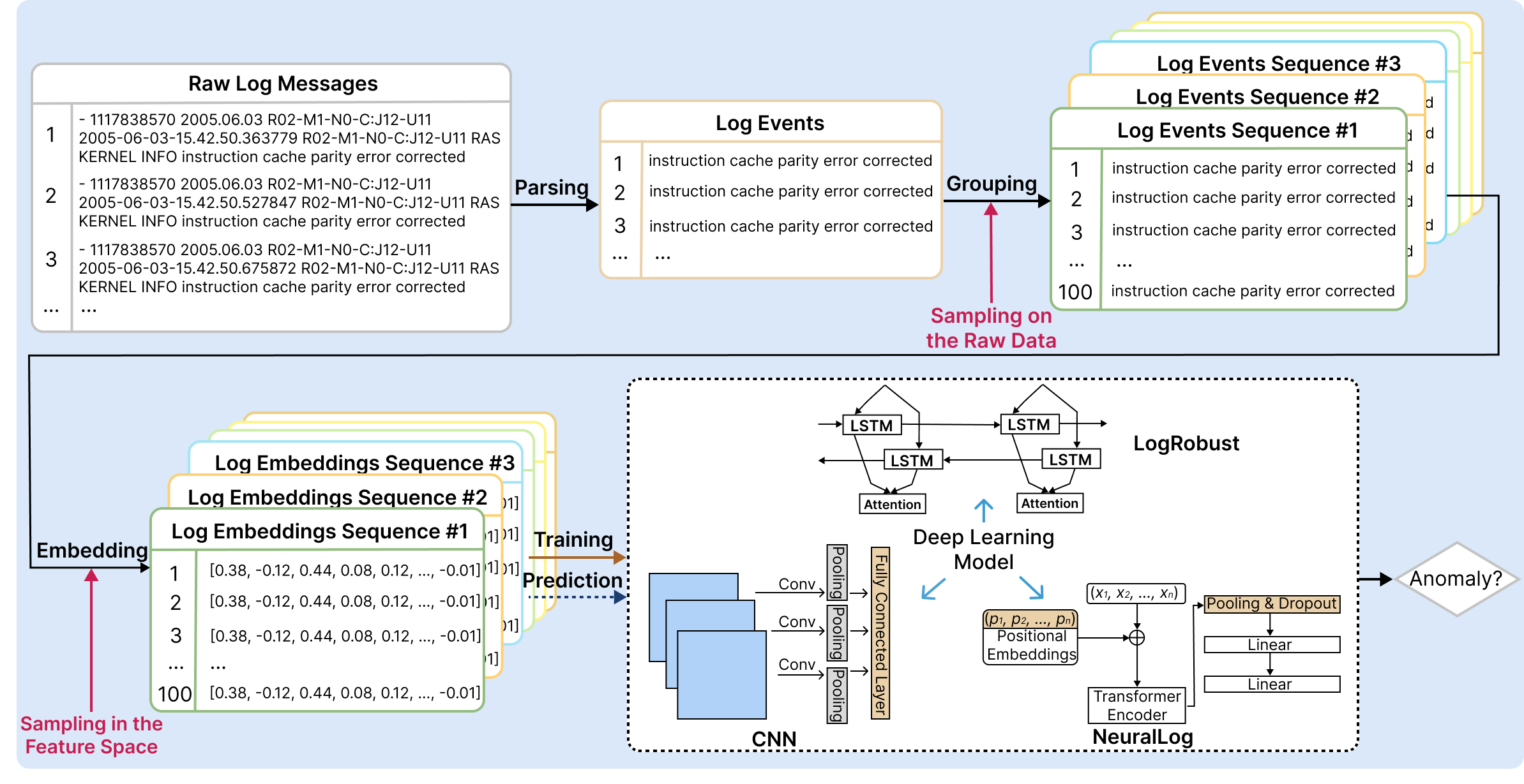
Figure 1: The common workflow of DLLAD approaches.

To effectively extract valuable information for analysis, previous studies [19, 8, 10, 11, 2] convert the unstructured log messages generated during system operation into structured log events. Each log message comprises a header and content, where the header includes information like timestamps, typically omitted from analysis [2]. The log content is then segmented into constant and variable sections [2]. By replacing variable elements with a special symbol, the original log messages are converted into log events as illustrated in Figure 1. To group log events into log sequences, we adopt the fixed window strategy used in prior studies [8, 11, 12]. If an abnormal log event is part of a log sequence, the log sequence is labeled as abnormal. Conversely, if the log sequence comprises solely normal log events, it is labeled as normal. These log sequences are subsequently transformed into embedding vectors and used as input for training a classification model to predict whether a log sequence is abnormal.

II-B Existing DLLAD Approaches

Recent DL approaches for anomaly detection can be categorized into three main groups (as discussed in Section VI): Convolutional Neural Network (CNN)-based models, Long Short-Term Memory-based models, and Transformer-based models. To select the most suitable DLLAD approaches, we take two factors into consideration. Firstly, we look for models that are representative of the DL models described in Section VI. Secondly, we aim to include models that have been recently proposed. Therefore, we choose the following models:

CNN. Lu et al. [9] adopted a CNN-based model to automatically detect log anomalies. Logs were parsed based on log keys, which were then encoded using logkey2vec. These embeddings were structured into a trainable matrix, simplifying neural network training. The model architecture comprised three convolutional layers, a dropout layer, and max-pooling layers.

LogRobust. Zhang et al. [10] employed Drain [20] for log parsing and integrated the FastText [21], a pre-trained Word2vec model, with TF-IDF weights [22] to represent log events as semantic vectors. Subsequently, these vectors are utilized as input to an attention-based Bi-directional LSTM (Bi-LSTM) model for detecting anomalies.

NeuralLog. Le et al. [2] preprocessed log messages without log parsing and encoded them into vector representations via a pre-trained Transformer-based language model BERT [23]. Then, they apply a transformer encoder to classify log sequences, with the primary objective of capturing semantic information comprehensively.

II-C Data Resampling

We make use of commonly adopted data resampling methods in the software engineering domain [24, 25, 26, 27]. These methods are classified into three primary categories: oversampling, undersampling, and hybrid sampling. As depicted by two arrows in Figure 1, certain resampling methods are tailored for use exclusively within the feature space, while others, such as random oversampling and undersampling [25], can be applied to both the raw data and the feature space. Data resampling methods applied to raw data focus on directly modifying the distribution of log sequences in the training set to address class imbalance, thereby altering the number of log sequences belonging to each class and subsequently impacting the embedding vectors derived from them. In contrast, data resampling methods within the feature space involve first embedding the original log sequences and then resampling based on these embedding vectors.

(1) Random OverSampling (ROS) randomly replicates log sequences of the minority class without generating new ones. These replicated abnormal sequences are then added to the original dataset. This method, when applied to raw data and feature space, is denoted as ROS_R and ROS_F, respectively.

(2) Random UnderSampling (RUS) randomly selects log sequences from the majority class and subsequently removes them from the original dataset. This method, when applied to raw data and feature space, is denoted as RUS_R and RUS_F, respectively.

(3) Synthetic Minority Oversampling Technique (SMOTE) [14] is an oversampling method applied to the feature space. It augments the minority class by generating synthetic log sequences instead of duplications. This method first randomly selects log sequences from the minority class. For each selected abnormal log sequence $M_{A}$, one of its $k$ nearest neighbors $M_{B}$ are randomly chosen. The embedding vector of the synthetic log sequence $M_{S}$ is calculated with the formula $x_{s}=x_{A}+Random(0,1)(x_{B}-x_{A})$, where $x_{A}$ and $x_{B}$ represent the embedding vectors of $M_{A}$ and $M_{B}$, separately. These newly generated synthetic abnormal log sequences are subsequently added to the original dataset.

(4) Adaptive Synthetic Sampling Approach [15] (ADASYN) serves as an extension of SMOTE. Unlike SMOTE, ADASYN generates new synthetic abnormal log sequences near the class boundary instead of within the abnormal log sequences themselves.

(5) NearMiss [16] operates as an undersampling method. It calculates the distance between two classes and randomly removes normal log sequences based on the distance. In our evaluation, we adopt NearMiss-3, which has demonstrated superior performance compared to NearMiss-1 and NearMiss-2. Specifically, NearMiss-3 selects a number of the nearest normal log sequences for each abnormal log sequence and removes them from the dataset.

(6) Instance Hardness Threshold (IHT) [17] involves the application of a classifier to the dataset, followed by the removal of log sequences that are hard to classify. The Random Forest (RF) [28] algorithm serves as the default estimator for estimating the Instance Hardness (IH) [17] of individual log sequences.

(7) SMOTEENN [18] is a hybrid sampling method that combines the oversampling method SMOTE and the undersampling method Edited Nearest Neighbour (ENN) [29]. SMOTE generates abnormal log sequences that can sometimes overlap with the majority class, making classification challenging. ENN, acting as a data cleaning method, helps address this issue. For a normal log sequence, if more than half of its $k$ neighbor log sequences do not belong to the majority class, then the log sequence is removed.

(8) SMOTETomek [18] is a hybrid sampling method that shares similarities with SMOTEENN. It incorporates Tomek links [30] for data cleaning, defined by the distances between log sequences $M_{i}$ and $M_{j}$ from different two classes. A pair ($M_{i}$, $M_{j}$) forms a Tomek link if no log sequence $M$ exists with $d(M_{i},M)<d(M_{i},M_{j})$ or $d(M_{j},M)<d(M_{i},M_{j})$. After oversampling by SMOTE, the log sequences that form Tomek links are then removed to help reduce potential noise or borderline log sequences that may affect classification performance.

III Study Design

III-A Datasets

To assess the performance of the log anomaly detection approaches with the data resampling methods, there are four widely-used publicly available datasets [31, 32], namely HDFS, BGL, Thunderbird, and Spirit. However, since most existing approaches (e.g., LogRobust and NeuralLog) have already achieved satisfactory results on the HDFS dataset (e.g., F1 exceeding 0.98), we exclude it from our evaluation. BGL dataset [31] is a collection of supercomputing system log data gathered by Lawrence Livermore National Labs. Thunderbird and Spirit datasets [31] are acquired from two real-world supercomputers at Sandia National Labs. These log datasets consist of both normal and abnormal log messages, which have been manually identified.

TABLE I: The statistics of the three public datasets. TB, $Msg$, $Seq$, and $A$ are the abbreviations of Thunderbird, Messages, Sequences, and Anomalies, respectively.

Dataset	# of $Msg$	$ws$	Training Data		Testing Data
			# of $Seq$	# of $A$	# of $Seq$	# of $A$
BGL	4,713,493	20	188,540	17,252	47,134	3,006
		50	75,416	7,415	18,853	1,383
		100	37,708	4,009	9,425	817
TB	5,000,000	20	200,000	328	50,000	37
		50	79,999	195	19,999	29
		100	39,999	138	9,999	23
Spirit	5,000,000	20	200,000	8,817	50,000	290
		50	79,999	4,275	19,999	270
		100	39,999	2,577	9,999	250

To group log events into a log sequence, a fixed window grouping strategy is commonly used [8, 11, 12]. However, choosing an appropriate window size ($ws$) is challenging. A small $ws$ makes it difficult for log anomaly detection models to capture anomalies that span multiple log sequences [1]. Additionally, employing smaller $ws$ results in more log sequences containing fewer log events, ultimately leading to slower training speed. On the other hand, if $ws$ is large, log sequences may include multiple anomalies and confuse the detection scheme [1, 33]. In the majority of prior research studies [8, 11, 2, 12, 34], a single window size is typically employed to evaluate the proposed approaches, with $ws$=20 being the most common choice. A few studies [1, 13] have investigated multiple window sizes including 20, 100, and 200. In most cases, the F1 performance is found to be better at $ws$=20 and 100 compared to $ws$=200. However, there is no consistent pattern regarding which performs better between $ws$=20 and $ws$=100. Our experiment results (shown in Table III) also emphasize the absence of a universally optimal window size across all DLLAD datasets. For instance, LogRobust exhibits superior F1 and MCC performance on the Thunderbird dataset at $ws$=100, while achieving better performance on other datasets at $ws$=20. As a result, in our experiments, we consider both $ws$=20 and $ws$=100 as window sizes to account for potential variations in performance. Additionally, we introduce a $ws$ of 50 to provide a balanced perspective between the shorter and longer sequences analyzed. By including this intermediate window size, we aim to uncover a more nuanced understanding of how log sequence length impacts DLLAD performance, and whether the effects of data resampling across datasets with different window sizes are robust.

In Table I, we present the number of log sequences (# of Sequences) in each dataset across various window sizes, as well as recording the number of abnormal sequences within all sequences (# of Anomalies) in both the training and test sets. In Table II, we report the proportions of abnormal sequences within all sequences (% of Anomalies) before and after employing data resampling methods. The proportions of anomalies are determined based on the resampling ratios of normal to abnormal log sequences, which are calculated by multiplying the original ratio of normal to abnormal log sequences by quarter-based constants. The original datasets exhibit very small proportions of anomalies, ranging from 0.16% to 10.63%. Moreover, enlarging the window size has minimal impact on the level of class imbalance across each dataset (for example, in BGL, the proportion of abnormal sequences is 9.15% with $ws$=20 and 10.63% with $ws$=100.). Upon implementing the specified resampling ratios, the proportions of abnormal sequences have shown increases: 9.15% to 40.29% (BGL dataset with $ws$=20), 9.83% to 43.62% (BGL dataset with $ws$=50), 10.63% to 49.33% (BGL dataset with $ws$=100), 0.16% to 0.66% (Thunderbird dataset with $ws$=20), 0.24% to 0.98% (Thunderbird dataset with $ws$=50), 0.35% to 1.38% (Thunderbird dataset with $ws$=100), 4.41% to 18.50% (Spirit dataset with $ws$=20), 5.34% to 22.58% (Spirit dataset with $ws$=50), 6.44% to 27.55% (Spirit dataset with $ws$=100), respectively.

TABLE II: The proportion of abnormal sequences within all log sequences before and after over-/under-/hybrid sampling. $r$ denotes the original ratio of normal to abnormal log sequences in the training dataset, and quarter-based constants are represented as 1/4, 1/2, and 3/4. The last nine columns correspond to the proportion of abnormal sequences after data resampling.

Dataset	$ws$	% of Anomalies	% of Anomalies After Oversampling			% of Anomalies After Undersampling			% of Anomalies After hybrid sampling
			r*1/4	r*1/2	r*3/4	r*1/4	r*1/2	r*3/4	r*1/4	r*1/2	r*3/4
BGL	20	9.15%	40.29%	20.14%	13.43%	28.72%	16.77%	11.84%	38.84%	19.36%	12.90%
	50	9.83%	43.62%	21.81%	14.54%	30.37%	17.90%	12.69%	43.27%	21.62%	14.39%
	100	10.63%	47.59%	23.79%	15.86%	32.24%	19.22%	13.69%	49.33%	21.98%	13.53%
TB	20	0.16%	0.66%	0.33%	0.22%	0.65%	0.33%	0.22%	0.58%	0.29%	0.20%
	50	0.24%	0.98%	0.49%	0.33%	0.97%	0.49%	0.32%	0.85%	0.43%	0.32%
	100	0.35%	1.38%	0.69%	0.46%	1.37%	0.69%	0.46%	1.36%	0.67%	0.46%
Spirit	20	4.41%	18.45%	9.22%	6.15%	15.57%	8.44%	5.79%	18.50%	9.20%	6.17%
	50	5.34%	22.58%	11.29%	7.53%	18.42%	10.15%	7.00%	17.70%	10.50%	7.81%
	100	6.44%	27.55%	13.77%	9.18%	21.60%	12.11%	8.41%	22.44%	11.16%	7.39%

III-B Evaluation

We use four commonly used evaluation metrics Recall, Precision, Specificity, and F1-score in previous DLLAD studies [12, 2, 1, 35]. Given that Matthews Correlation Coefficient (MCC) and Area Under the Curve (AUC) are recommended for evaluating software engineering tasks with class imbalance [36, 37, 38, 39, 40], we include both MCC and AUC in our evaluation to provide a comprehensive assessment of DLLAD model performance. The commonly used four metrics originate from the confusion matrix, which describes four types of instances: TP (True Positives) represents the number of abnormal log sequences correctly predicted as anomalies, TN (True Negatives) represents the number of normal log sequences correctly predicted as normal, FP (False Positives) represents the number of normal log sequences incorrectly predicted as anomalies, and FN (False Negatives) represents the number of abnormal log sequences incorrectly predicted as normal. The definitions of these metrics are as follows:

(1) Recall$=\frac{TP}{TP+FN}$ represents the proportion of actual anomalies that are correctly predicted by DLLAD models out of all actual anomalies present in the testing dataset. It indicates DLLAD models’ ability to capture all abnormal log sequences correctly.

(2) Precision$=\frac{TP}{TP+FP}$ measures the proportion of predicted anomalies by DLLAD models that are actual anomalies out of all anomalies predicted by the models. It indicates the accuracy of the DLLAD models in identifying actual anomalies without falsely labeling normal log sequences as anomalies.

(3) Specificity$=\frac{TN}{TN+FP}$ represents the proportion of actual normal log sequences that are correctly predicted as normal by DLLAD models out of all actual normal log sequences. It indicates the ability of the DLLAD models to correctly identify normal log sequences as normal.

(4) F1-score$=\frac{2\times(Recall\times Precision)}{Recall+Precision}$ calculates the harmonic mean of Recall and Precision. It provides a balanced measure between Precision and Recall, giving equal weight to false positives and false negatives.

(5) MCC$=\frac{TP\times TN-FP\times FN}{\sqrt{(TP+FP)(TP+FN)(TN+FP)(TN+FN)}}$ is a fully symmetric metric that takes into account all four values (TP, TN, FP, and FN) in the confusion matrix when calculating the correlation between ground truth and predicted values.

(6) AUC is a threshold-independent measure that can be calculated by assessing the area under the Receiver Operating Characteristic (ROC) curve, which plots the true positive rate (Sensitivity) against the false positive rate (1 - Specificity) at various threshold settings. Unlike other metrics such as Precision, Recall, F1-score, and MCC, which depend on the choice of a threshold, AUC evaluates the classifier’s performance across all possible threshold values.

To determine the statistical significance of the observed performance differences among these data resampling methods, we employ the Scott-Knott Effect Size Difference (ESD) test [41] based on the assumptions of ANalysis Of VAriance (ANOVA). The Scott-Knott ESD test is a multiple comparison approach that leverages hierarchical clustering to partition these data resampling methods into distinct groups, exhibiting statistically significant differences at the predetermined significance level of 0.05 ($\alpha$=0.05). There are no statistically significant differences between data resampling methods within the same group, but significant differences are observed between data resampling methods located in different groups.

III-C Research Questions

RQ1. Do the existing DLLAD approaches perform well enough with varying degrees of class imbalance? In this RQ, we evaluate the performance of existing DLLAD approaches in detecting log sequence anomalies across datasets with different levels of class imbalance. Specifically, our objective is to understand whether significant differences in class imbalance have a notable influence on the effectiveness of these DLLAD approaches. In cases where the achieved performance is unsatisfactory, especially when dealing with extreme class imbalance, the utilization of data resampling methods becomes essential to address data imbalance issues prior to model training. Consequently, in RQ2, our primary focus is to explore the optimal resampling ratios of normal to abnormal data. Subsequently, based on these ratios, in RQ3, we discuss the effectiveness of data resampling methods in enhancing the capabilities of DLLAD models.

RQ2. How does the resampling ratio of normal to abnormal data affect the ability of data resampling? Due to the varying levels of class imbalance in the different datasets, it is challenging to establish a fixed resampling ratio of normal to abnormal data, such as maintaining a consistent 10:1 ratio of normal to abnormal log sequences across all datasets. Conducting an exhaustive exploration of countless potential ratios to identify an optimal resampling ratio for each dataset is not practically feasible. Considering the substantial data imbalance, we avoid pursuing a 1:1 ratio of normal to abnormal data during the data resampling process. This is particularly evident in the Thunderbird dataset, where the training set has a mere 0.16% anomaly rate with a window size of 20. Applying a 1:1 ratio in such cases would result in excessive data removal during undersampling, leading to a significant loss of information. Thus, this resampling ratio is not considered. Instead, we adopt the quarter as a foundational unit for our empirical investigations in a flexible and adaptive manner, as shown in Table II.

RQ3. Does data resampling improve the effectiveness of existing DLLAD approaches? In this RQ, we utilize the recommended resampling ratios of normal to abnormal data observed in RQ2 within evaluated data resampling methods. Subsequently, we assess the effectiveness of these resampling methods when applied to existing DLLAD approaches.

III-D Implementations

We implement the existing approaches introduced in Section II-B using their respective GitHub repositories or reproduced codebases. Following previous works [2, 1], in our dataset setup, the training set comprises the first 80% of raw logs, while the remaining 20% is allocated for testing. To reduce computational complexity and memory demands during data resampling operations, for NeuralLog [2], we reduce the embedding dimension from 768 to 256. For CNN [9] and LogRobust [10], we utilize the implementations [1], adhering to the instructions provided by the authors. The implementation of data resampling methods is carried out using the Python toolbox [42] Imbalanced-learn. Our experiments encompass 27 distinct instances, resulting from the combination of 3 DLLAD approaches, 3 datasets, and 3 window sizes. For each experimental instance, we investigate 10 data resampling methods with 3 different resampling ratios of normal to abnormal data and NoSampling. As a result, we have a total of 3 $\times$ 3 $\times$ 3 $\times$ ( 10 $\times$ 3 $+$ 1) combinations, summing up to 837 unique scenarios. To mitigate the variations in performance across different runs, we perform five runs for each data resampling method (including NoSampling), culminating in a total of 4,185 experiments conducted in this study. These five-run results are utilized for statistical significance analysis using the Scott-Knott ESD test, which calculates the group ranking of each data resampling method across different datasets. Furthermore, the averages of the five-run results are provided in Tables III–VI in Section IV. We run our experiments on a Linux server with an Intel Xeon Silver 4210 CPU and four Nvidia GeForce RTX 3090-Ti GPUs.

IV Results and Analysis

IV-A RQ1. Do the existing DLLAD approaches perform well enough with varying degrees of class imbalance?

Table III provides an overview of the performance of CNN, LogRobust, and NeuralLog on the BGL, Thunderbird, and Spirit datasets with three window sizes. On the BGL and Thunderbird datasets, the best values for all evaluation metrics are attained with a window size of 20 or 50. Specifically, on the BGL dataset, except for NeuralLog achieving the highest Precision and Specificity with $ws$=50, setting $ws$=20 yields the best values for all evaluation metrics. Regarding the Thunderbird dataset, LogRobust exhibits notably low precision with $ws$=20, resulting in subpar performance in terms of F1 and MCC. However, LogRobust demonstrates better performance with $ws$=50 than $ws$=100 in terms of all evaluation metrics. CNN and NeuralLog follow a similar pattern, with all evaluation metrics achieving optimal results when $ws$=20, except for NeuralLog achieving the highest AUC with $ws$=50. On the Spirit dataset, CNN achieves similar performance with $ws$=20 and $ws$=100 in terms of F1 and MCC, outperforming $ws$=50. LogRobust’s best performance is observed with $ws$=20 in terms of Precision, Specificity, F1, and MCC, while LogRobust performs best in Recall and AUC with $ws$=100. NeuralLog demonstrates comparable performance with $ws$=20 and 50, with slight variations $\textless$ 0.001 in Specificity, F1, and MCC, but superior to $ws$=100.

Regarding the Thunderbird dataset, it is notable that all three approaches demonstrate relatively poor performance, particularly CNN and LogRobust, which exhibit F1 and MCC values below 0.5. Although NeuralLog performs better with an F1 of 0.760 at $ws$=20, its performance remains unsatisfactory. This subpar performance may be attributed to the dataset’s extreme imbalance across three window sizes, compromising the models’ ability to accurately detect both normal and abnormal log sequences.

TABLE III: The Recall, Precision, Specificity, F1-score, MCC, and AUC values of the three DLLAD approaches across the three datasets, each with three different window sizes. Bold font highlights the best performance among the three window sizes.

		BGL			TB			Spirit
Model	Metric	$ws$=20	$ws$=50	$ws$=100	$ws$=20	$ws$=50	$ws$=100	$ws$=20	$ws$=50	$ws$=100
CNN	R	0.948	0.907	0.916	0.495	0.460	0.304	0.815	0.893	0.909
	P	0.985	0.708	0.362	0.443	0.169	0.213	0.797	0.582	0.726
	S	0.999	0.965	0.827	0.999	0.997	0.997	0.999	0.991	0.991
	F1	0.966	0.787	0.510	0.441	0.247	0.241	0.806	0.704	0.807
	MCC	0.964	0.779	0.509	0.454	0.277	0.247	0.805	0.716	0.807
	AUC	0.977	0.919	0.903	0.866	0.812	0.786	0.967	0.996	0.995
LogRobust	R	0.949	0.911	0.903	0.766	0.609	0.449	0.892	0.910	0.918
	P	0.860	0.709	0.793	0.084	0.317	0.277	0.973	0.805	0.863
	S	0.989	0.968	0.978	0.994	0.998	0.997	1.000	0.997	0.994
	F1	0.903	0.792	0.844	0.151	0.415	0.340	0.930	0.832	0.889
	MCC	0.897	0.783	0.831	0.252	0.437	0.350	0.931	0.854	0.885
	AUC	0.970	0.960	0.954	0.915	0.861	0.826	0.991	0.990	0.997
NeuralLog	R	0.896	0.627	0.598	0.772	0.730	0.756	0.899	0.931	0.938
	P	0.852	0.872	0.671	0.758	0.469	0.470	0.899	0.864	0.800
	S	0.989	0.991	0.878	1.000	0.999	0.999	0.999	0.999	0.999
	F1	0.872	0.721	0.496	0.760	0.571	0.579	0.895	0.896	0.862
	MCC	0.864	0.718	0.511	0.762	0.585	0.596	0.897	0.896	0.865
	AUC	0.943	0.809	0.738	0.856	0.865	0.828	0.949	0.965	0.964

IV-B RQ2. How does the resampling ratio of normal to abnormal data affect the ability of data resampling?

We comprehensively evaluate the ten data resampling methods for each dataset using quarter-based resampling ratios obtained by multiplying the original ratio of normal data to abnormal data by 1/4, 1/2, and 3/4, as described in Section III-A. The employed data resampling methods are categorized into three distinct groups: OverSampling (comprising SMOTE, ADASYN, ROS_F, and ROS_R), UnderSampling (encompassing NearMiss, IHT, RUS_F, and RUS_R), and HybridSampling, represented by SMOTEENN and SMOTETomek. In Figure 2, the three DLLAD approaches utilizing the ten data resampling methods with the three resampling ratios are described through heatmaps, with a special focus on the MCC metric, since MCC is a fully symmetric metric that takes into account all four values (TP, TN, FP, and FN) in the confusion matrix. We adopt an enumeration of “hits”, signifying instances where a particular resampling ratio maximizes the performance of these DLLAD approaches.

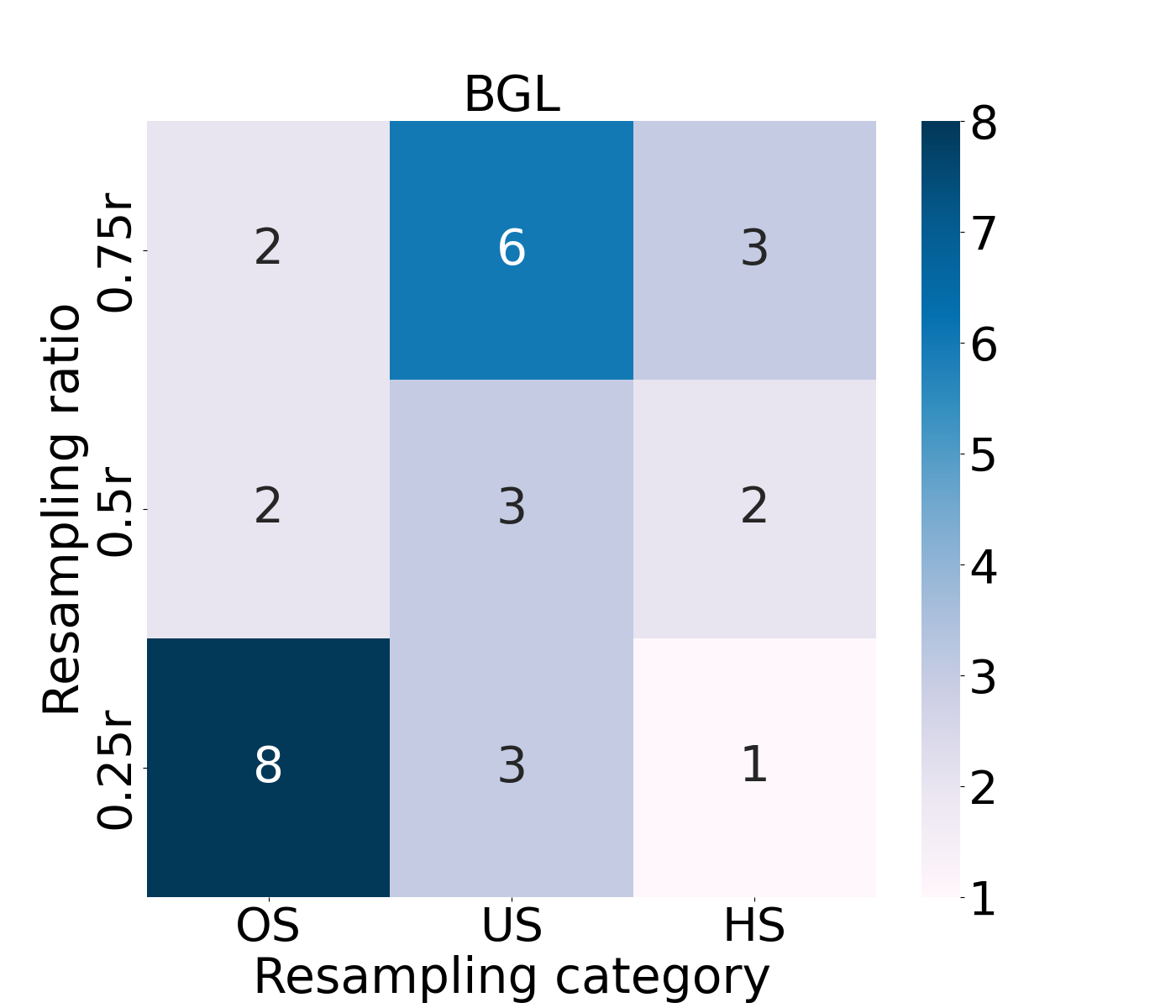
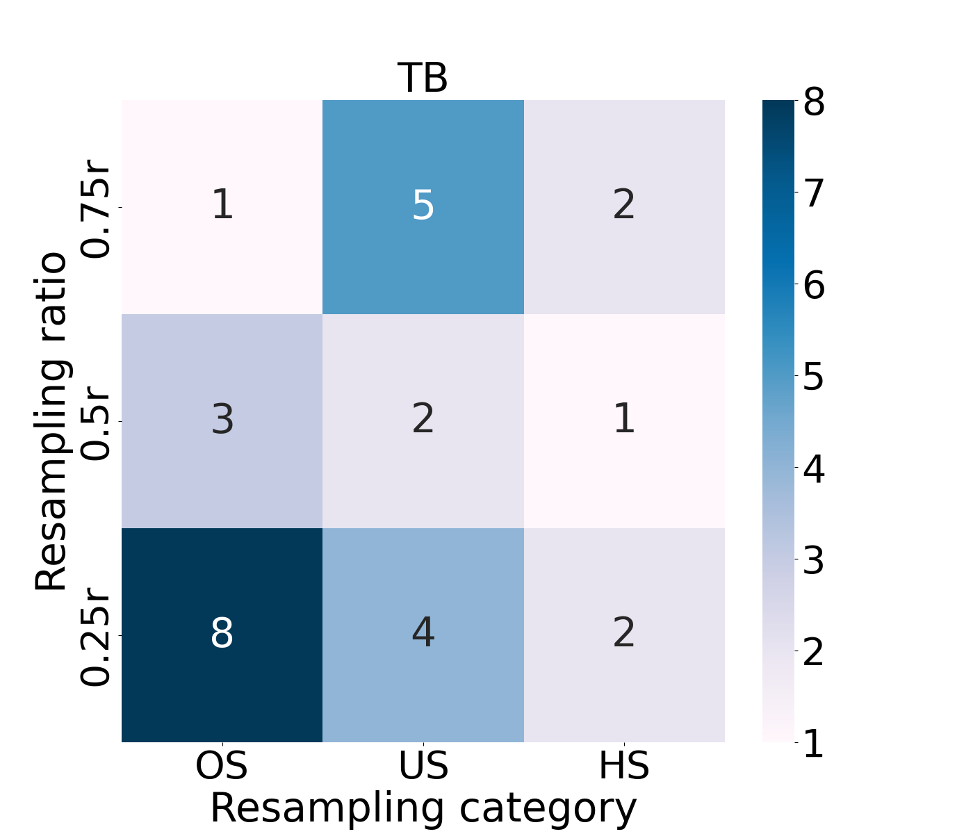
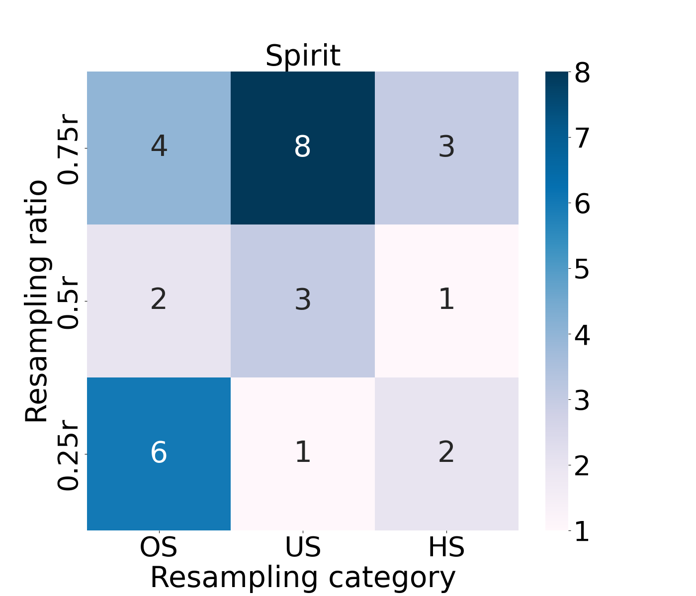
(a) $ws$=20

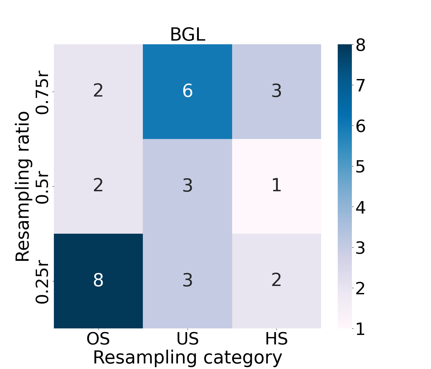
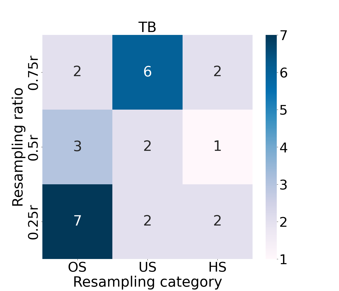
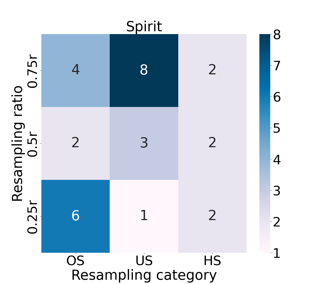
(b) $ws$=50

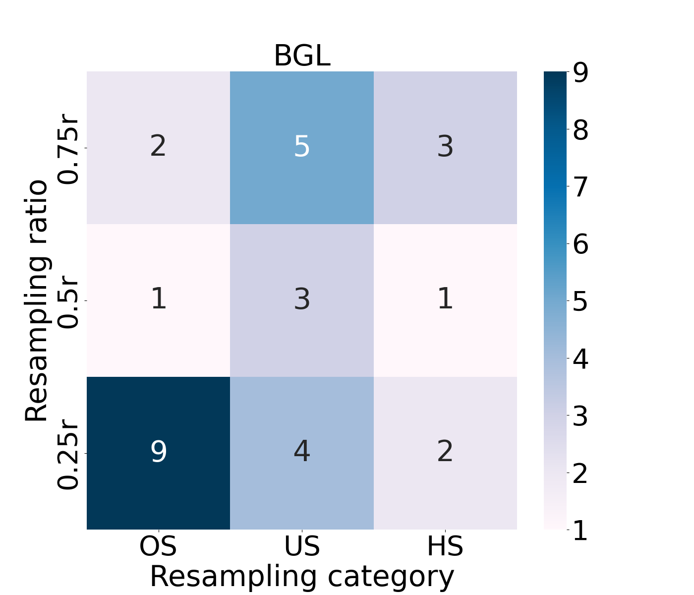
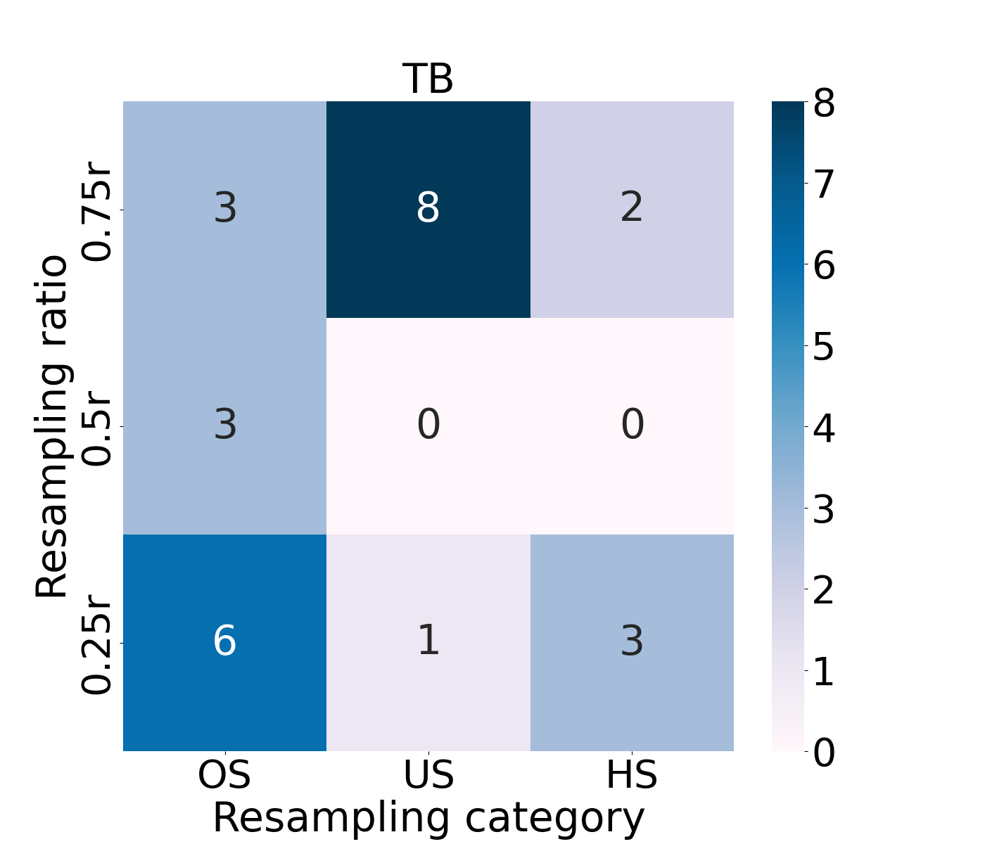
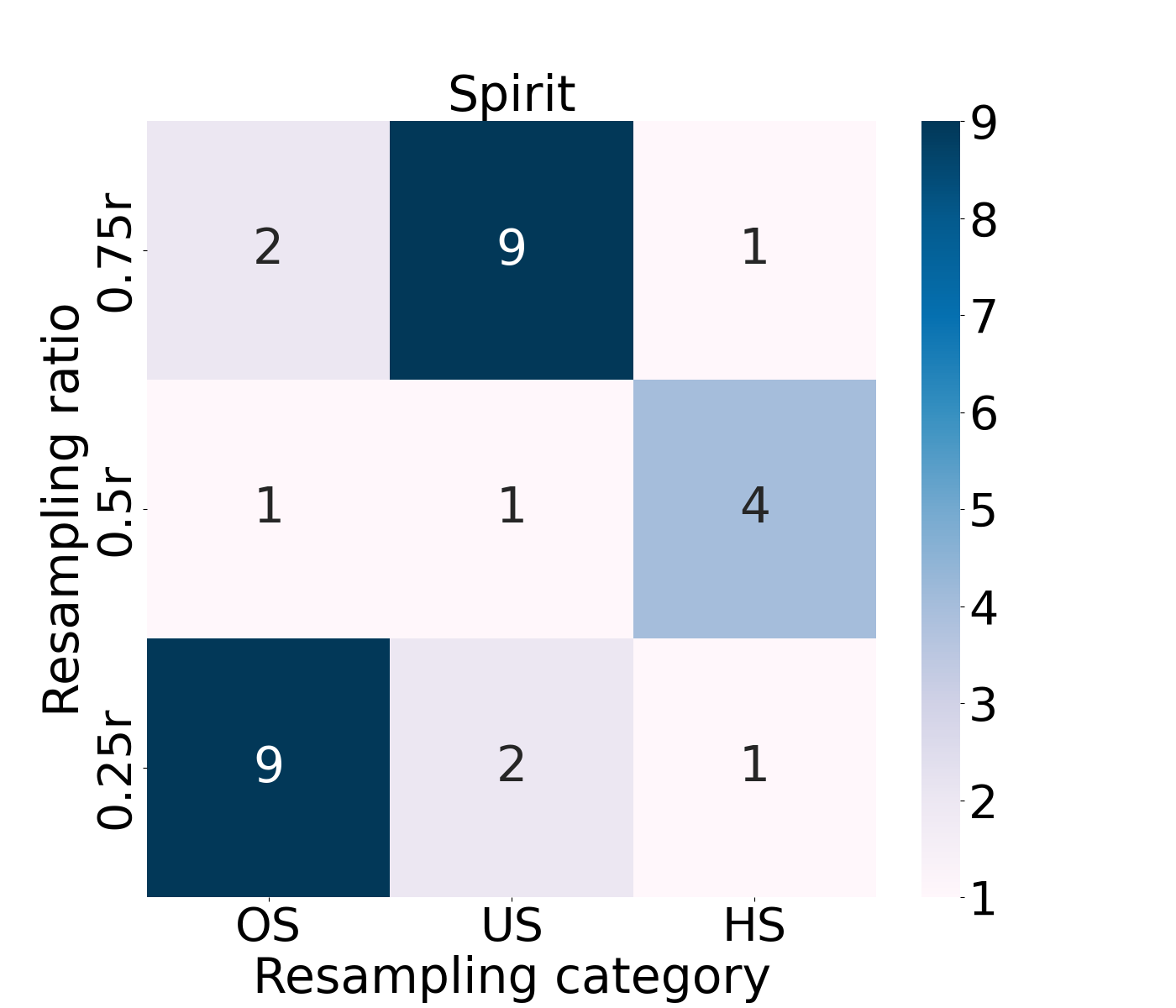
(c) $ws$=100

Figure 2: The heatmap depicting the statistics of the best performance of the data resampling methods (including OverSampling (OS), UnderSampling (US), and HybridSampling (HS)) with the three resampling ratios ($r$ representing the original ratio of normal to abnormal data) across the three datasets with different window sizes. (a) $ws$=20. (b) $ws$=50. (c) $ws$=100.

In Figures 2–2, the analytical scope centers on three datasets that use the same window size of 20. As an illustrative example, the MCC values for NeuralLog’s performance using SMOTE with three resampling ratios on the BGL dataset ($ws$=20) are 0.947, 0.939, and 0.937, respectively. In this specific case, the resampling ratio equal to one-quarter of the original data ratio of normal to abnormal data yields the highest MCC value. Consequently, a “hit” is recorded for the corresponding entry, aligning with the cell marked with a count of 8 in the lower left corner. If all three MCC values were identical, there would be no hits recorded. In Figure 2, oversampling methods demonstrate superior performance when the resampling ratio is one-quarter of the original ratio of normal to abnormal data. This phenomenon is particularly pronounced in BGL and Thunderbird datasets, both yielding 8 hits out of a total of 12. Regarding the Spirit dataset, the DLLAD approaches with NoSampling exhibit strong performance in accurately detecting anomalies, with the MCC ranging from 0.716 to 0.931. Interestingly, for this dataset, the selected resampling ratio of normal to abnormal data appears to have less impact on the performance of oversampling methods. When considering undersampling methods, removing a smaller amount of original normal log sequences can enhance the effectiveness of these methods. This effect is particularly prominent when examining the Spirit dataset, yielding 8 out of 12 hits. For hybrid sampling methods, it is difficult to determine the most appropriate resampling ratio of normal to abnormal data for the studied approaches. Especially in the Thunderbird dataset, both one-quarter and three-quarter resampling ratios exhibit an equal likelihood of achieving the best DLLAD performance.

In Figures 2 and 2, our findings exhibit a remarkable consistency with those presented in Figure 2. When the resampling ratio is set to one-quarter of the original ratio of normal to abnormal data, employing oversampling methods on the three datasets demonstrates the highest likelihood of achieving optimal performance, particularly in the BGL dataset, with 8 or 9 out of 12 hits. Conversely, when the resampling ratio is adjusted to three-quarters of the original ratio of normal to abnormal data, the effectiveness of undersampling methods is maximized. This is notable in the Spirit dataset, where 8 or 9 out of 12 hits are observed, signifying optimal performance. Concerning hybrid sampling methods, offering robust recommendations regarding the optimal resampling ratio of normal to abnormal data remains a challenging task. The effectiveness varies inconsistently across the three datasets. Specifically, the most suitable resampling ratio within the predefined range is three-quarters of the original ratio for the BGL dataset, one-quarter of the original ratio for the Thunderbird dataset, and one-second of the original ratio for the Spirit dataset, respectively.

The effectiveness of this finding is mainly attributed to two aspects: 1) the introduction of diverse features through extensive oversampling of abnormal log sequences, and 2) the retention of valuable information from the original data while efficiently removing a limited number of normal log sequences. Oversampling and undersampling under these specific conditions contribute to enhancing the classification capabilities of DLLAD approaches.

IV-C RQ3. Does data resampling improve the effectiveness of existing DLLAD approaches?

TABLE IV: The Recall, Precision, Specificity, F1-score, MCC, and AUC values of CNN when employing various data resampling methods (i.e., NoSampling (NS), SMOTE (SMO), ADASYN (ADA), NearMiss (NM), InstanceHardnessThreshold (IHT), SMOTEENN (SE), SMOTETomek (ST), RandomOverSampling in the feature space (ROS_F), RandomUnderSampling in the feature space (RUS_F), RandomOverSampling applied to raw data (ROS_R), and RandomUnderSampling applied to raw data (RUS_R)) to the three datasets, each with the three different window sizes. Darker cells signify superior performance, while various colors denote statistical significance among data resampling methods for each evaluation metric (determined by the Scott-Knott ESD test with a $p$-value$\textless$0.05), as observed in the subsequent tables.

Dataset	$ws$	Metric	NS	SMO	ADA	NM	IHT	SE	ST	ROSF	RUSF	ROSR	RUSR
		R	0.948	0.963	0.962	0.956	0.967	0.961	0.962	0.962	0.960	0.961	0.961
		P	0.985	0.978	0.982	0.989	0.945	0.995	0.989	0.984	0.986	0.984	0.986
		S	0.999	0.999	0.999	0.999	0.996	1.000	0.999	0.999	0.999	0.992	0.999
		F1	0.966	0.970	0.972	0.972	0.956	0.977	0.975	0.973	0.973	0.972	0.974
		MCC	0.964	0.968	0.970	0.970	0.953	0.976	0.973	0.971	0.971	0.972	0.972
	20	AUC	0.977	0.982	0.978	0.978	0.974	0.977	0.979	0.984	0.974	0.984	0.983
		R	0.907	0.910	0.912	0.898	0.944	0.896	0.915	0.931	0.915	0.918	0.899
		P	0.708	0.853	0.877	0.895	0.192	0.882	0.761	0.538	0.205	0.885	0.885
		S	0.965	0.987	0.990	0.991	0.684	0.990	0.971	0.916	0.717	0.990	0.991
		F1	0.787	0.880	0.894	0.896	0.319	0.888	0.820	0.665	0.335	0.901	0.892
		MCC	0.779	0.871	0.886	0.888	0.341	0.880	0.814	0.665	0.352	0.893	0.883
	50	AUC	0.919	0.941	0.959	0.952	0.824	0.937	0.943	0.929	0.857	0.944	0.951
		R	0.916	0.930	0.900	0.911	0.937	0.894	0.902	0.927	0.901	0.907	0.898
		P	0.362	0.857	0.832	0.923	0.218	0.885	0.665	0.905	0.798	0.928	0.613
		S	0.827	0.996	0.983	0.993	0.681	0.989	0.920	0.991	0.977	0.993	0.945
		F1	0.510	0.891	0.865	0.917	0.353	0.888	0.729	0.916	0.844	0.917	0.727
		MCC	0.509	0.889	0.852	0.909	0.359	0.878	0.722	0.908	0.831	0.910	0.713
BGL	100	AUC	0.903	0.962	0.928	0.958	0.837	0.953	0.912	0.954	0.929	0.953	0.907
		R	0.495	0.495	0.532	0.532	0.550	0.000	0.495	0.568	0.541	0.550	0.495
		P	0.443	0.821	0.426	0.123	0.185	1.000	0.821	0.154	0.230	0.825	0.817
		S	0.999	1.000	0.999	0.997	0.998	1.000	1.000	0.998	0.998	1.000	1.000
		F1	0.441	0.618	0.443	0.198	0.274	0.000	0.618	0.241	0.315	0.659	0.613
		MCC	0.454	0.637	0.460	0.253	0.316	0.000	0.638	0.293	0.347	0.673	0.634
	20	AUC	0.866	0.840	0.873	0.880	0.894	0.545	0.839	0.894	0.865	0.881	0.843
		R	0.460	0.379	0.414	0.000	0.391	0.000	0.345	0.402	0.000	0.345	0.000
		P	0.169	0.800	0.315	0.000	0.255	0.000	0.537	0.481	0.000	0.923	0.000
		S	0.997	1.000	0.999	1.000	0.998	1.000	0.999	0.999	1.000	1.000	1.000
		F1	0.247	0.490	0.355	0.000	0.299	0.000	0.383	0.376	0.000	0.501	0.000
		MCC	0.277	0.536	0.359	0.000	0.309	0.000	0.410	0.406	0.000	0.563	0.000
	50	AUC	0.812	0.799	0.826	0.713	0.816	0.638	0.793	0.810	0.725	0.841	0.738
		R	0.304	0.290	0.348	0.043	0.261	0.000	0.319	0.348	0.000	0.348	0.000
		P	0.213	0.326	0.447	0.333	0.092	0.000	0.465	0.463	0.000	0.600	0.000
		S	0.997	0.998	0.999	1.000	0.996	1.000	0.998	0.999	1.000	0.999	1.000
		F1	0.241	0.276	0.391	0.077	0.136	0.000	0.334	0.397	0.000	0.420	0.000
		MCC	0.247	0.290	0.393	0.120	0.153	0.000	0.360	0.400	0.000	0.444	0.000
TB	100	AUC	0.786	0.788	0.776	0.736	0.786	0.656	0.788	0.801	0.733	0.802	0.730
		R	0.815	0.822	0.814	0.822	0.851	0.614	0.823	0.826	0.808	0.823	0.800
		P	0.797	0.922	0.864	0.797	0.482	0.845	0.934	0.975	0.975	0.991	0.946
		S	0.999	1.000	0.999	0.999	0.995	0.999	1.000	1.000	1.000	1.000	1.000
		F1	0.806	0.868	0.837	0.806	0.615	0.646	0.875	0.894	0.884	0.899	0.866
		MCC	0.805	0.869	0.837	0.807	0.638	0.681	0.876	0.897	0.887	0.902	0.869
	20	AUC	0.967	0.969	0.968	0.968	0.974	0.963	0.969	0.971	0.973	0.972	0.971
		R	0.893	0.907	0.888	0.908	0.963	0.065	0.893	0.935	0.903	0.908	0.889
		P	0.582	0.677	0.769	0.415	0.243	0.080	0.592	0.873	0.510	0.786	0.618
		S	0.991	0.994	0.996	0.983	0.959	0.990	0.992	0.998	0.988	0.997	0.992
		F1	0.704	0.774	0.823	0.570	0.388	0.071	0.712	0.903	0.652	0.842	0.728
		MCC	0.716	0.780	0.823	0.607	0.472	0.060	0.723	0.902	0.673	0.842	0.737
	50	AUC	0.996	0.997	0.997	0.993	0.978	0.921	0.996	0.998	0.995	0.998	0.997
		R	0.909	0.919	0.919	0.899	0.961	0.888	0.908	0.931	0.907	0.925	0.924
		P	0.726	0.853	0.771	0.510	0.311	0.623	0.657	0.904	0.784	0.880	0.803
		S	0.991	0.996	0.993	0.977	0.945	0.986	0.988	0.997	0.994	0.997	0.994
		F1	0.807	0.882	0.838	0.649	0.470	0.730	0.762	0.917	0.841	0.902	0.858
		MCC	0.807	0.881	0.837	0.666	0.530	0.735	0.765	0.915	0.839	0.899	0.857
Spirit	100	AUC	0.995	0.998	0.998	0.992	0.976	0.994	0.997	0.999	0.988	0.998	0.988

TABLE V: The Recall, Precision, Specificity, F1-score, MCC, and AUC values of LogRobust when employing various data resampling methods to the three datasets, each with the three different window sizes.

Dataset	$ws$	Metric	NS	SMO	ADA	NM	IHT	SE	ST	ROSF	RUSF	ROSR	RUSR
		R	0.949	0.958	0.955	0.951	0.952	0.952	0.956	0.938	0.942	0.951	0.948
		P	0.860	0.885	0.889	0.882	0.858	0.887	0.889	0.892	0.892	0.912	0.904
		S	0.989	0.992	0.992	0.991	0.989	0.992	0.992	0.992	0.992	0.994	0.993
		F1	0.903	0.920	0.921	0.915	0.903	0.918	0.921	0.914	0.916	0.931	0.925
		MCC	0.897	0.915	0.916	0.910	0.897	0.913	0.916	0.909	0.911	0.926	0.920
	20	AUC	0.970	0.985	0.988	0.980	0.974	0.983	0.982	0.974	0.975	0.980	0.982
		R	0.911	0.901	0.920	0.871	0.940	0.944	0.904	0.919	0.901	0.901	0.898
		P	0.709	0.895	0.879	0.648	0.565	0.821	0.823	0.891	0.872	0.902	0.896
		S	0.968	0.992	0.990	0.953	0.942	0.983	0.983	0.991	0.989	0.992	0.992
		F1	0.792	0.898	0.899	0.726	0.706	0.877	0.859	0.905	0.886	0.901	0.897
		MCC	0.783	0.890	0.891	0.718	0.703	0.869	0.849	0.897	0.877	0.893	0.889
	50	AUC	0.960	0.966	0.966	0.964	0.962	0.960	0.942	0.966	0.965	0.963	0.966
		R	0.903	0.928	0.878	0.917	0.945	0.887	0.908	0.889	0.900	0.936	0.887
		P	0.793	0.892	0.908	0.870	0.803	0.896	0.957	0.914	0.900	0.894	0.896
		S	0.978	0.989	0.992	0.987	0.978	0.990	0.996	0.992	0.990	0.989	0.990
		F1	0.844	0.909	0.892	0.893	0.868	0.892	0.932	0.901	0.900	0.915	0.892
		MCC	0.831	0.901	0.882	0.883	0.858	0.882	0.926	0.892	0.890	0.907	0.882
BGL	100	AUC	0.954	0.963	0.961	0.959	0.961	0.961	0.971	0.967	0.964	0.966	0.961
		R	0.766	0.459	0.641	0.775	0.811	0.000	0.775	0.802	0.703	0.652	0.529
		P	0.084	0.708	0.218	0.108	0.127	0.000	0.111	0.141	0.313	0.285	0.352
		S	0.994	1.000	0.998	0.995	0.996	1.000	0.995	0.996	0.997	0.998	0.998
		F1	0.151	0.532	0.313	0.189	0.220	0.000	0.193	0.239	0.368	0.376	0.371
		MCC	0.252	0.557	0.364	0.286	0.319	0.000	0.290	0.335	0.425	0.415	0.403
	20	AUC	0.915	0.849	0.903	0.920	0.933	0.544	0.916	0.922	0.905	0.685	0.870
		R	0.609	0.529	0.598	0.347	0.644	0.000	0.540	0.552	0.425	0.598	0.425
		P	0.317	0.804	0.433	0.647	0.236	0.000	0.271	0.404	0.636	0.852	0.805
		S	0.998	1.000	0.999	1.000	0.996	1.000	0.998	0.998	1.000	1.000	1.000
		F1	0.415	0.637	0.481	0.450	0.333	0.000	0.355	0.444	0.497	0.703	0.554
		MCC	0.437	0.651	0.497	0.473	0.379	0.000	0.378	0.459	0.513	0.713	0.583
	50	AUC	0.861	0.881	0.864	0.847	0.885	0.524	0.872	0.854	0.860	0.870	0.865
		R	0.449	0.464	0.435	0.536	0.565	0.029	0.485	0.435	0.507	0.464	0.420
		P	0.277	0.436	0.510	0.216	0.146	0.667	0.374	0.597	0.469	0.655	0.488
		S	0.997	0.998	0.999	0.995	0.992	1.000	0.998	0.999	0.999	0.999	0.999
		F1	0.340	0.429	0.457	0.297	0.232	0.056	0.418	0.501	0.484	0.526	0.450
		MCC	0.350	0.438	0.463	0.331	0.284	0.139	0.422	0.507	0.485	0.541	0.451
TB	100	AUC	0.826	0.868	0.846	0.851	0.848	0.727	0.859	0.865	0.864	0.831	0.837
		R	0.892	0.910	0.914	0.910	0.937	0.791	0.913	0.913	0.915	0.918	0.915
		P	0.973	0.991	0.990	0.836	0.510	0.547	0.975	0.993	0.996	0.990	0.989
		S	1.000	1.000	1.000	0.999	0.995	0.992	1.000	1.000	1.000	1.000	1.000
		F1	0.930	0.949	0.950	0.862	0.660	0.542	0.943	0.951	0.954	0.953	0.950
		MCC	0.931	0.950	0.951	0.867	0.689	0.599	0.943	0.951	0.954	0.953	0.951
	20	AUC	0.991	0.990	0.993	0.988	0.991	0.980	0.992	0.993	0.994	0.993	0.992
		R	0.910	0.903	0.914	0.896	0.974	0.899	0.903	0.907	0.910	0.925	0.907
		P	0.805	0.949	0.763	0.736	0.218	0.717	0.893	0.957	0.884	0.905	0.917
		S	0.997	0.999	0.996	0.996	0.952	0.995	0.999	0.999	0.998	0.999	0.999
		F1	0.832	0.925	0.832	0.808	0.356	0.798	0.898	0.931	0.897	0.915	0.912
		MCC	0.854	0.925	0.833	0.809	0.449	0.800	0.897	0.930	0.896	0.914	0.911
	50	AUC	0.990	0.990	0.990	0.989	0.967	0.989	0.990	0.990	0.990	0.991	0.990
		R	0.918	0.923	0.920	0.925	0.981	0.765	0.913	0.939	0.923	0.909	0.916
		P	0.863	0.945	0.904	0.609	0.330	0.725	0.644	0.972	0.895	0.983	0.950
		S	0.994	0.999	0.996	0.984	0.949	0.991	0.987	0.999	0.997	1.000	0.999
		F1	0.889	0.933	0.911	0.733	0.493	0.717	0.753	0.955	0.908	0.945	0.932
		MCC	0.885	0.932	0.908	0.742	0.553	0.725	0.759	0.954	0.906	0.944	0.931
Spirit	100	AUC	0.996	0.999	0.997	0.993	0.982	0.994	0.995	0.998	0.997	0.997	0.996

TABLE VI: The Recall, Precision, Specificity, F1-score, MCC, and AUC values of NeuralLog when employing various data resampling methods to the three datasets, each with the three different window sizes.

Dataset	$ws$	Metric	NS	SMO	ADA	NM	IHT	SE	ST	ROSF	RUSF	ROSR	RUSR
		R	0.896	0.951	0.929	0.842	0.766	0.867	0.875	0.939	0.897	0.937	0.925
		P	0.852	0.932	0.908	0.166	0.818	0.908	0.925	0.894	0.958	0.923	0.910
		S	0.989	0.995	0.994	0.691	0.987	0.994	0.995	0.992	0.997	0.995	0.994
		F1	0.872	0.941	0.918	0.275	0.788	0.886	0.899	0.915	0.926	0.930	0.917
		MCC	0.864	0.937	0.913	0.282	0.776	0.880	0.893	0.910	0.922	0.925	0.912
	20	AUC	0.943	0.971	0.956	0.767	0.877	0.930	0.935	0.966	0.947	0.966	0.955
		R	0.627	0.753	0.891	0.755	0.732	0.645	0.675	0.899	0.680	0.880	0.807
		P	0.872	0.825	0.840	0.284	0.740	0.900	0.888	0.844	0.956	0.897	0.903
		S	0.991	0.985	0.984	0.621	0.979	0.992	0.990	0.986	0.998	0.992	0.992
		F1	0.721	0.770	0.854	0.325	0.735	0.739	0.747	0.869	0.794	0.888	0.837
		MCC	0.718	0.763	0.849	0.297	0.715	0.740	0.749	0.860	0.794	0.879	0.836
	50	AUC	0.809	0.869	0.937	0.688	0.856	0.819	0.833	0.943	0.839	0.936	0.899
		R	0.598	0.892	0.828	0.640	0.874	0.755	0.713	0.842	0.520	0.878	0.656
		P	0.671	0.715	0.831	0.323	0.190	0.799	0.887	0.883	0.808	0.879	0.904
		S	0.878	0.963	0.982	0.601	0.650	0.980	0.991	0.989	0.985	0.989	0.993
		F1	0.496	0.787	0.818	0.336	0.312	0.767	0.789	0.859	0.603	0.878	0.759
		MCC	0.511	0.774	0.807	0.259	0.300	0.751	0.778	0.848	0.608	0.866	0.752
BGL	100	AUC	0.738	0.919	0.916	0.620	0.763	0.890	0.852	0.905	0.753	0.927	0.829
		R	0.772	0.862	0.561	0.821	0.683	0.496	0.691	0.772	0.683	0.756	0.740
		P	0.758	0.800	0.852	0.717	0.825	0.886	0.869	0.842	0.886	0.942	0.883
		S	1.000	1.000	1.000	1.000	1.000	1.000	1.000	1.000	1.000	1.000	1.000
		F1	0.760	0.827	0.676	0.765	0.738	0.635	0.770	0.805	0.771	0.838	0.805
		MCC	0.762	0.829	0.691	0.766	0.745	0.662	0.775	0.806	0.778	0.843	0.808
	20	AUC	0.856	0.931	0.780	0.910	0.841	0.748	0.845	0.886	0.841	0.886	0.878
		R	0.730	0.854	0.805	0.854	0.748	0.537	0.748	0.813	0.813	0.879	0.715
		P	0.469	0.788	0.797	0.700	0.803	0.880	0.671	0.808	0.603	0.986	0.935
		S	0.999	1.000	1.000	1.000	1.000	1.000	1.000	1.000	0.999	1.000	1.000
		F1	0.571	0.812	0.797	0.769	0.770	0.667	0.686	0.808	0.683	0.928	0.811
		MCC	0.585	0.816	0.799	0.773	0.773	0.687	0.697	0.809	0.695	0.930	0.818
	50	AUC	0.865	0.927	0.902	0.927	0.874	0.768	0.874	0.906	0.906	0.939	0.899
		R	0.756	0.756	0.911	0.683	0.732	0.512	0.618	0.805	0.780	0.813	0.732
		P	0.470	0.697	0.497	0.583	0.698	0.778	0.790	0.750	0.681	0.828	0.882
		S	0.999	1.000	0.999	1.000	1.000	1.000	1.000	1.000	1.000	1.000	1.000
		F1	0.579	0.718	0.641	0.629	0.714	0.618	0.642	0.776	0.727	0.820	0.800
		MCC	0.596	0.722	0.671	0.631	0.714	0.631	0.672	0.777	0.729	0.820	0.803
TB	100	AUC	0.828	0.878	0.955	0.841	0.866	0.756	0.832	0.902	0.890	0.906	0.866
		R	0.899	0.919	0.929	0.950	0.940	0.881	0.925	0.939	0.920	0.919	0.924
		P	0.899	0.969	0.902	0.380	0.510	0.976	0.945	0.928	0.800	0.976	0.889
		S	0.999	1.000	0.999	0.990	0.995	1.000	1.000	1.000	0.999	1.000	0.999
		F1	0.895	0.943	0.915	0.534	0.661	0.925	0.935	0.933	0.855	0.946	0.905
		MCC	0.897	0.943	0.915	0.591	0.690	0.927	0.935	0.933	0.857	0.947	0.905
	20	AUC	0.949	0.959	0.964	0.970	0.968	0.940	0.962	0.969	0.960	0.960	0.962
		R	0.931	0.913	0.937	0.944	0.946	0.889	0.919	0.932	0.933	0.923	0.919
		P	0.864	0.975	0.921	0.446	0.588	0.969	0.957	0.947	0.921	0.997	0.997
		S	0.999	1.000	1.000	0.993	0.996	1.000	1.000	1.000	1.000	1.000	1.000
		F1	0.896	0.943	0.929	0.603	0.724	0.926	0.937	0.939	0.927	0.959	0.957
		MCC	0.896	0.943	0.928	0.644	0.743	0.927	0.937	0.939	0.926	0.959	0.957
	50	AUC	0.965	0.962	0.968	0.968	0.971	0.944	0.960	0.966	0.966	0.962	0.961
		R	0.938	0.930	0.937	0.829	0.951	0.853	0.937	0.923	0.926	0.937	0.937
		P	0.800	0.985	0.989	0.810	0.556	0.938	0.927	0.989	0.974	0.996	0.947
		S	0.999	1.000	1.000	1.000	0.996	1.000	1.000	1.000	1.000	1.000	1.000
		F1	0.862	0.957	0.962	0.819	0.702	0.893	0.932	0.955	0.950	0.966	0.942
		MCC	0.865	0.957	0.962	0.819	0.726	0.894	0.932	0.955	0.950	0.966	0.941
Spirit	100	AUC	0.964	0.965	0.968	0.915	0.973	0.926	0.968	0.961	0.963	0.968	0.964

Tables IV–VI present the results of the three DLLAD approaches with ten data resampling methods and NoSampling on the three datasets. We utilize three distinct colors to underscore the statistical differences among data resampling methods and NoSampling in terms of all evaluation metrics: Recall, Precision, Specificity, F1, MCC, and AUC. These methods are categorized into multiple groups using the Scott-Knott ESD test, often resulting in more than six groups. Darker colors indicate higher-ranked groups, with each color representing two groups (i.e., the darkest purple denotes the first and second groups, moderate purple indicates the third and fourth groups, and the lightest purple represents the fifth and sixth groups). If some data resampling methods fall outside the top six groups but significantly outperform NoSampling, the results of these data resampling methods will be bolded.

In general, our analysis reveals consistent patterns in the performance of ten data resampling methods across different DLLAD approaches in terms of comprehensive metrics F1, MCC, and AUC. For instance, in Table IV, oversampling methods (SMOTE and ADASYN) and the oversampling method ROS_R applied to raw data, significantly enhance the overall performance of CNN across datasets, with improvements ranging from 0.1% to 102.7% in F1, 0.5% to 103.2% in MCC, and 0.1% to 6.6% in AUC. Table V illustrates that utilizing SMOTE, ROS_F, and RUS_F within the feature space, in addition to the resampling methods applied directly to raw data (ROS_R and RUS_R), leads to significant performance improvements for LogRobust across all datasets. These methods demonstrate notable enhancements in F1 (improved by 1.3% to 252.3%), MCC (improved by 1.3% to 121.0%), and AUC (improved by 0.3% to 5.1%). Additionally, in many cases, ADASYN and SMOTETomek significantly perform better than NoSampling. Similarly, Table VI highlights the effectiveness of data resampling for NeuralLog. Most data resampling methods, including SMOTE, SMOTETomek, ROS_F, ROS_R, and RUS_R, can achieve significantly better performance than NoSampling across all datasets with improvements ranging from 1.1% to 77.0% in F1, 1.8% to 69.5% in MCC, and 0.1% to 25.6% in AUC. In summary, SMOTE, ROS_F, ROS_R, and RUS_R applied to DLLAD approaches significantly outperform NoSampling. Additionally, improvements are observed in other metrics such as Recall and Precision.

In addition, we observe that employing ROS_R on all three DLLAD approaches consistently yields superior performance. Specifically, ROS_R ranks within the top two groups (represented by the darkest purple color) in all 27 cases (3 DLLAD approaches $\times$ 3 datasets $\times$ 3 window sizes) in terms of at least two comprehensive metrics. SMOTE emerges as the second recommended data resampling method, demonstrating significantly better performance than NoSampling in 26 out of 27 cases across all datasets in terms of at least two comprehensive metrics. Similarly, ROS_F and RUS_R outperform NoSampling in 25 out of 27 cases, followed by ADASYN in 24 out of 27 cases. In contrast, NearMiss, IHT, and SMOTEENN exhibit poor performance, succeeding in only 10 out of 27, 4 out of 27, and 13 out of 27 cases, respectively.

In datasets characterized by moderate imbalance, such as BGL and Spirit, several data resampling methods contribute to improved performance in DLLAD approaches. Given the consistent results between F1 and MCC, and the minimal changes in AUC in certain cases, our analysis primarily focuses on the outcomes of MCC, a recommended symmetric metric. For the BGL dataset with a $ws$ of 20, CNN achieves high performance with an MCC of 0.964 (as shown in Table IV). Most data resampling methods, excluding IHT, contribute to a slight improvement of 0.4%–1.2%. When the $ws$ is set to 100, the impact of data resampling methods becomes more significant, with enhancements ranging from 40.1% to 78.8%. The Recall is increased by the reduction in false positives, leading to a higher percentage of accurately predicted anomalies and an overall enhancement in the comprehensive metric MCC. With $ws$=50, IHT, ROS_F, and RUS_F perform inferiorly to NoSampling, while others improve NoSampling by 5.5%–14.6%. Similarly, for the same dataset with $ws$=20, most data resampling methods, except for IHT, enhance the performance of LogRobust (Table V), with improvements ranging from 1.3% to 3.2%. At $ws$=50, aside from undersampling methods applied to the feature space (i.e., NearMiss and IHT), all other methods positively impact the performance, with improvements of 8.4%–14.6%. At $ws$=100, all data resampling methods enhance NoSampling with an increase of 3.2%–11.4%. In the case of NeuralLog, data resampling methods consistently show improvement trends, as shown in Table VI. Except for NearMiss and IHT, all other resampling methods lead to improvements ranging from 1.9% to 69.5% across three window sizes.

For the Spirit dataset with $ws$=20, Table IV illustrates that most data resampling methods, except for NearMiss, IHT, and SMOTEENN, contribute to an improvement in the performance of CNN, with enhancements ranging from 4.0% to 12.0% in MCC. With $ws$=50, except for NearMiss, IHT, SMOTEENN, and RUS_R, other methods show positive effects, resulting in improvements of 1.0% to 26.0%. At $ws$=100, except for NearMiss, IHT, SMOTEENN, and SMOTETomek, other methods enhance NoSampling by 3.7% to 13.4%. Table V indicates that data resampling on LogRobust has a comparable impact to data resampling on CNN. With the exception of undersampling and hybrid sampling methods applied within the feature space, other methods excluding ADASYN contribute to an increase in NoSampling by 1.3% to 8.9% across three window sizes. When applying data resampling to NeuralLog, only NearMiss, IHT, and RUS_F do not enhance its performance across window sizes, as demonstrated in Table VI. Other data resampling methods show improvements of 0.9% to 11.7% compared to NoSampling.

In the highly imbalanced Thunderbird dataset, both ROS_R and SMOTE demonstrate overall performance enhancements for DLLAD approaches, with ROS_R showing statistically significant improvements across all cases. When applying data resampling methods to CNN on this dataset, unexpected results appear. Undersampling methods, such as RUS_F, RUS_R, NearMiss, as well as the hybrid sampling method SMOTEENN, uniformly cause the CNN to classify all log sequences as normal sequences, resulting in performance metrics (i.e., Recall, Precision, F1, and MCC) being reduced to 0. Conversely, ROS_R improves NoSampling by 48.2%, 103.2%, and 79.8% for $ws$ set to 20, 50, and 100, respectively. Surprisingly, a statistically significant difference in CNN performance is only observed with SMOTETomek and ROS_R. Table V demonstrates that when applying data resampling to LogRobust on this dataset, all data resampling methods except for NearMiss, IHT, SMOTEENN, and SMOTETomek yield improvements ranging from 5.0% to 121.0% across three window sizes. In contrast to the effects observed on CNN, it is worth noting that undersampling, oversampling, and hybrid sampling methods except for ADASYN, IHT, and SMOTEENN, can positively impact NeuralLog (as shown in Table VI). Particularly, random sampling applied to raw data (i.e., ROS_R and RUS_R) substantially enhances the MCC of NoSampling by 6.0% to 59.0%. In addition, concerning other metrics such as Recall and Precision, data resampling methods (except for NearMiss, IHT, and SMOTEENN) significantly outperform NoSampling across all datasets in most cases.

Furthermore, there are other noteworthy observations from the analysis. Some undersampling methods (i.e., NearMiss and IHT) might not perform well in many cases, particularly in the dataset with severe class imbalance. The limited performance of these methods can be attributed to the significant reduction of the majority class while addressing class imbalance. This reduction poses a risk of losing vital information present in the log data. Hybrid sampling methods like SMOTEENN attempt to address class imbalance by generating synthetic abnormal sequences and subsequently eliminating normal log sequences that share overlapping features with another class. Similarly, SMOTEENN cannot effectively improve the performance of DLLAD approaches. One potential reason for this limitation is that removing normal log sequences based on overlapping features between the synthetic abnormal sequences (which may contain noise) and the normal data may also result in the loss of crucial information. In contrast, oversampling methods, which focus on generating additional log sequences of the minority class, effectively mitigate the class imbalance issue. While this process may introduce some level of noise due to the replication and generation of abnormal log sequences, it seems to be a more effective strategy for preserving crucial information within log data. These observations emphasize the trade-off between addressing class imbalance and retaining critical data information when applying the data resampling methods in DLLAD.

V Discussion

V-A Why Do(not) Data Resampling Methods Work?

TABLE VII: An example of an abnormal log sequence from the Spirit dataset with $ws$=20, where the second log event is highlighted in orange as it represents an anomaly (left), and the top five tokens in the log sequence contributing to the DLLAD model’s correct prediction are highlighted in orange (right).

#	Log event	Top five tokens
1	publickey for $<*>$ from $<*>$ port $<*>$ ssh$<*>$	NoSampling : publickey, opened, closed, port, user
2	LANai is not running. Allowing port=$<*>$ open for debugging	SMOTE : publickey, debugging, LANai, opened, user
3	NOTICE: $<*>$
4	closed for user $<*>$	ADASYN : publickey, debugging, opened, user, ssh
5	opened for user $<*>$ by $<*>$
6	publickey for $<*>$ from $<*>$ port $<*>$ ssh$<*>$	NearMiss : publickey, opened, closed, user, debugging
7	opened for user $<*>$ by $<*>$
8	publickey for $<*>$ from $<*>$ port $<*>$ ssh$<*>$	IHT : publickey, debugging, LANai, opened, user
9	opened for user $<*>$ by $<*>$
10	publickey for $<*>$ from $<*>$ port $<*>$ ssh$<*>$	SMOTEENN : publickey, closed, opened, user, NOTICE
11	opened for user $<*>$ by $<*>$
12	publickey for $<*>$ from $<*>$ port $<*>$ ssh$<*>$	SMOTETomek : publickey, opened, NOTICE, debugging, closed
13	opened for user $<*>$ by $<*>$
14	publickey for $<*>$ from $<*>$ port $<*>$ ssh$<*>$	ROSF : publickey, debugging, NOTICE, LANai, closed
15	opened for user $<*>$ by $<*>$
16	publickey for $<*>$ from $<*>$ port $<*>$ ssh$<*>$	RUSF : publickey, debugging, LANai, NOTICE, closed
17	opened for user $<*>$ by $<*>$
18	publickey for $<*>$ from $<*>$ port $<*>$ ssh$<*>$	ROSR : debugging, port, open, publickey, NOTICE
19	opened for user $<*>$ by $<*>$
20	publickey for $<*>$ from $<*>$ port $<*>$ ssh$<*>$	RUSR : debugging, NOTICE, port, user, publickey

TABLE VIII: An example of a normal log sequence from the Thunderbird dataset with $ws$=20, along with the top five tokens in the log sequence contributing to the DLLAD model’s prediction (right).

#	Log event	Top five tokens
1	client does not accept options	NoSampling : client, no, free, leases, options
2	client does not accept options	SMOTE : client, options, Temperature, changed, stratum
3	client does not accept options
4	client does not accept options	ADASYN : client, options, Temperature, Celsius, stratum
5	client does not accept options
6	from $<*>$ via eth1: network $<*>$ no free leases	NearMiss : client, options, no, free, leases
7	from $<*>$ via eth1: network $<*>$ no free leases
8	/dev/sda, Temperature changed $<*>$ Celsius to $<*>$ Celsius since last report	IHT : client, options, Temperature, stratum, network
9	/dev/sda, Temperature changed $<*>$ Celsius to $<*>$ Celsius since last report
10	to $<*>$ stratum $<*>$	SMOTEENN : client, options, Celsius, Temperature, network
11	to $<*>$ stratum $<*>$
12	to $<*>$ stratum $<*>$	SMOTETomek : client, options, Celsius, Temperature, stratum
13	/dev/sda, Temperature changed $<*>$ Celsius to $<*>$ Celsius since last report
14	client does not accept options	ROSF : client, options, Temperature, Celsius, stratum
15	client does not accept options
16	client does not accept options	RUSF : client, options, Celsius, Temperature, stratum
17	client does not accept options
18	client does not accept options	ROSR : client, options, Temperature, Celsius, stratum
19	client does not accept options
20	client does not accept options	RUSR : client, options, Temperature, Celsius, stratum

In RQ3, we investigate the impact of various data resampling methods on the performance of DLLAD approaches. To enhance the interpretability of their performance, we utilize Local Interpretable Model-agnostic Explanations (LIME) [43], which is a widely-used model-agnostic explainable algorithm for explaining deep learning models in software engineering [44, 45, 46, 47, 48, 49]. LIME can identify the most important tokens in a log sequence that contribute to the DLLAD model’s prediction.

In Tables VII and  VIII, we present two examples showcasing the LIME results for an actual abnormal and normal log sequence, both with and without employing data resampling methods. The first column denotes the number of log events in the log sequence, while the second column describes the specific content of each log event. The last column displays the top five tokens contributing to the LogRobust prediction with various data resampling methods. (1) The example in Table VII is derived from the Spirit dataset with $ws$=20, where certain data resampling methods perform better than NoSampling in terms of Recall. The second log event, highlighted in orange, signifies its abnormal nature. This event signifies the attempt to open a port for debugging purposes, which is typically considered an abnormal operation in a production environment. Such an action may suggest a potential security risk or an effort to troubleshoot an issue. LogRobust with NoSampling erroneously predicts the actual abnormal log sequence as normal. Examining the top five tokens reveals none of them appearing in the abnormal log event, thereby failing to accurately capture any abnormal information. However, when employing data resampling methods except for SMOTEENN, LogRobust correctly predicts the abnormal sequence based on highlighted abnormal tokens. Notably, with ROS_R, three tokens overlap with the abnormal log event, suggesting that properly duplicated log sequences in the raw data could positively influence DLLAD models in learning real patterns for detecting anomalies. (2) The example in Table VIII is derived from the Thunderbird dataset with $ws$=20, where certain data resampling methods substantially improve the Precision values compared to NoSampling. LogRobust with NoSampling erroneously predicts the actual normal log event as abnormal. The top five tokens extracted by LogRobust with NoSampling primarily focus on the sixth and seventh log events. These events describe the unavailability of an IP address for allocation. While this repetition of log messages may imply network configuration or capacity planning issues, it is important to consider that in a dynamically changing network environment, especially with a large number of temporary devices or clients, such occurrences may be anticipated. After employing data resampling methods, except for NearMiss, the LogRobust model shifts its attention to different tokens, such as “Temperature”, “changed”, and “Celsius”, and predicts the actual normal log event as normal. In summary, certain data resampling methods can prioritize crucial tokens in log sequences, aiding DLLAD models in making more accurate predictions than NoSampling. Consequently, DLLAD models utilizing data resampling methods demonstrate improved prediction capabilities for both abnormal and normal log sequences. These advancements may result from the enhanced distribution of training data achieved through data resampling methods, enabling the model to better distinguish between normal and abnormal log sequences based on learned patterns.

V-B Implications of Our Findings

The analysis of the experiments demonstrated the superiority of SMOTE, ROS_F, ROS_R, and RUS_R over other data resampling methods in most cases. The choice of window size and DLLAD model significantly influence the comparative outcomes. This research carries several practical implications for practitioners.

(1) Efficiency prioritization: Practitioners typically aim to efficiently train DLLAD models to identify log anomalies within a short timeframe. In this regard, CNN and LogRobust require less training time, and larger window sizes can notably reduce costly processing time. Additionally, applying ROS and RUS methods on raw data for data duplication and removal before embedding takes considerably less time than data resampling methods in feature spaces. Based on our experimental findings, LogRobust outperforms CNN overall. Hence, employing ROS_R and RUS_R with LogRobust is recommended for efficient prediction.

(2) Effectiveness prioritization: For non-urgently training DLLAD models to detect log anomalies, practitioners prioritize high accuracy in predicted results. In datasets with smaller window sizes and more balanced distributions (e.g., BGL and Spirit), the difference between LogRobust and NeuralLog is not significant. However, for highly imbalanced datasets (e.g., Thunderbird), NeuralLog noticeably outperforms LogRobust. Thus, it is advisable to adopt these data resampling methods (SMOTE, ROS_F, ROS_R, and RUS_R) with NeuralLog for effective prediction.

V-C Threats to Validity

(1) Limited models and datasets. One potential concern pertains to our selection of DLLAD approaches, we adapted existing supervised approaches for our empirical investigation. This choice is motivated by several factors: Semi-supervised approaches leverage only a fraction of normal logs, whereas unsupervised methods assume datasets lack labels, diverging from our fully supervised data scenario. Furthermore, some unsupervised and semi-supervised approaches share a model structure similar to NeuralLog, as observed in LAnoBERT [34] and Hades [35]. Previous empirical studies [2, 1] have consistently shown inferior performance of unsupervised and semi-supervised approaches compared to supervised ones. Hence, we deliberately include the latest supervised approaches as our evaluated DLLAD approaches. Another concern arises from the limited availability of datasets. Given that there are currently only several public datasets available (i.e., HDFS, BGL, Thunderbird, and Spirit), approaches have already demonstrated good performance on HDFS, we have chosen to exclusively use the remaining three datasets for our experimental analysis. In future work, we intend to investigate the generalizability of our conclusions across more datasets.

(2) Hyperparameter settings. The selection of an appropriate resampling ratio of normal to abnormal data constitutes a threat when assessing the effectiveness of data resampling methods. Considering numerous data resampling methods and the impracticality of evaluating all of them across diverse datasets with exhaustive resampling ratio variations, it is crucial to systematically choose the resampling ratio. To address this challenge, we introduce a standardized quarter-based unit for a consistent benchmark across various data resampling methods. On this basis, the general conclusions obtained aid researchers in narrowing their focus for subsequent study phases.

(3) Generalizability. To enhance the generalizability of our findings, we intentionally select three distinct categories encompassing a total of ten data resampling methods. These data resampling methods are systematically applied to three existing DLLAD approaches on publicly available datasets. Our objective does not compare the effectiveness of those DLLAD approaches but rather focuses on evaluating the capabilities of different data resampling methods applied to those approaches. As such, our findings aim to highlight general trends in how data resampling affects different DLLAD approaches, with the ultimate goal of offering valuable insights to inform future research endeavors.

VI Related Work

VI-A Deep Learning-Based Log Anomaly Detection

Numerous DLLAD models have been proposed and typically fall into several categories, including CNN-based, LSTM-based, and Transformer-based models. Lu et al. [9] employed CNN with three filters to extract local semantic information from log data. Zhang et al. [50], Du et al. [8], and Meng et al. [11] adopted LSTM [51] to capture long-term dependencies in log sequences and learn log patterns for predicting the next log. Vinayakumar et al. [52] employed a stacked-LSTM model to learn temporal patterns using sparse representations. Zhang et al. [10] proposed the LogRobust method that integrated the attention mechanism with a Bi-LSTM model, enabling comprehensive sequence information capture in both directions. Li et al. [53] employed a unified attention-based Bi-LSTM model to learn the patterns for sequential anomaly detection. Le et al. [2] introduced NeuralLog, utilizing BERT for embedding representation and a Transformer encoder for log anomaly detection classification. To the best of our knowledge, only the work by Le et al. [1] has highlighted that DLLAD models trained on highly imbalanced datasets exhibit low precision or recall values. Yet, there is currently no research exploring whether data resampling methods can mitigate class imbalance issues and improve DLLAD model performance. Subsequent work, such as unsupervised approach LAnoBERT [34], and semi-supervised approaches like PLELog [12], AdaLog [13], and Hades [35], have emerged to alleviate the potential difficulty of acquiring large labeled log datasets for training supervised learning models in log anomaly detection. However, we chose to focus on CNN [9], LogRobust [10], and NeuralLog [2] as the DLLAD models in our study, instead of these recently proposed semi-supervised or unsupervised methods. Our rationale behind this decision is based on the following reasons. (1) Different data scenarios: semi-supervised approaches use only a portion of the normal logs, and unsupervised approaches assume datasets have no labels, which differs from our fully supervised data hypothesis scenario. (2) Similar model structure: some unsupervised and semi-supervised approaches share a model structure similar to NeuralLog [2]. For example, LAnoBERT [34] employed pre-trained BERT for unsupervised learning with a masked language modeling loss function, and Hades utilized FastText for semantic vector representation and Transformer for classification. (3) Performance disparities: previous empirical studies [2, 1] have indicated notably inferior performance of unsupervised and semi-supervised approaches compared to supervised approaches.

VI-B Data Resampling for Software Engineering.

Data resampling has been widely applied to address the class imbalance issue in the field of software engineering, such as quality prediction [54], bug classification [55, 56], defect prediction [57, 26, 58, 59, 60, 39, 61, 62], and code smell detection [63, 64]. For example, Zheng et al. [55] analyzed the impact of six data resampling methods (e.g., SMOTE, Mahakil [65], and Rose [66]) on multiple classifiers for bug report classification. They found that the combination of Rose with random forest yielded the best performance. Bennin et al. [59] observed that while their investigated data resampling methods have no statistically significant effect on defect prioritization, these methods improve the defect classification performance with regard to Recall and G-mean. Subsequently, they [39] demonstrated that random undersampling and borderline-SMOTE are the more stable data resampling methods in software defect prediction. Li et al. [64] investigated the effects of 31 imbalanced learning methods on machine learning classifiers for code smell detection. Their study revealed varied impacts of these methods across different code smells, with deep forest consistently enhancing performance. Additionally, certain data resampling methods such as CNN, ENN, BSMOTE, and ROS showed superior performance compared to SMOTE. Differently from prior work, in the context of log anomaly detection, which poses unique challenges such as the need for careful selection of window sizes, our research conducts an extensive analysis to explore the influence of data resampling methods on model performance across various window sizes. Furthermore, our study delves into the effects of some data resampling methods on both raw data and the feature space, providing valuable insights for practitioners in this field.

VI-C Deep Learning-Based Anomaly Detection in Other Fields.

Deep learning-based anomaly detection is applicable not only in software log anomaly detection but also in diverse fields like fraud detection [67, 68, 69, 70], medical diagnosis [71, 72, 73, 74], manufacturing defect detection [75], and network intrusion detection [76]. While the workflow for anomaly detection in these domains shares similarities with the depicted Figure 1, specific data preprocessing steps, such as log parsing and grouping, may not be applicable. In these fields, class imbalance also presents a significant challenge that can affect the performance of anomaly detection models. Various data resampling methods have been employed to address this issue. For example, Heryadi et al. [67] utilized RUS on non-fraudulent transactions and adopted a hybrid CNN-LSTM model to capture both short and long-term financial transaction features. Similarly, Roy et al. [68] implemented RUS with a recommended resampling ratio [77] of 10:1 for non-fraudulent to fraudulent credit card transaction data, followed by an LSTM model for detecting fraud in credit card transactions. In medical anomaly detection, imbalanced datasets pose challenges, leading to sensitivity issues during supervised training [74]. Common strategies, such as data resampling and cost-sensitive training [72], are employed to mitigate these challenges. Li et al. [73] employed a CNN-based model with adjusted class weights to analyze phonocardiograms for abnormal heart sound detection. In network intrusion detection, Abdelkhalek et al. [76] proposed a data resampling approach combining ADASYN and Tomek Links in conjunction with diverse deep learning models (such as LSTM and CNN) for improved detection of malicious attacks, aiming to address the class imbalance issue between normal traffic and attack samples. In summary, the aforementioned studies suggest that certain data resampling methods can enhance model performance, aligning with our findings. However, empirical research regarding the most effective data resampling methods, optimal resampling ratio, and their impacts on both raw data and the feature space is currently lacking in these fields.

VII Conclusion

Our study represents a pioneering effort in comprehensively assessing the impact of ten data resampling methods on alleviating class imbalance in DLLAD. Through empirical analysis, we have derived several critical insights. Firstly, severe data imbalances, like in the Thunderbird dataset, often lead to poor performance in DLLAD approaches. Secondly, oversampling methods generally outperform both undersampling and hybrid sampling methods. Moreover, data resampling on raw data yields superior results compared to data resampling in the feature space. Notably, ROS_R exhibits outstanding performance, particularly in scenarios characterized by severe class imbalances. Thirdly, certain undersampling and hybrid sampling methods, such as SMOTEENN and IHT, show limited effectiveness in most cases. Furthermore, our exploration of different resampling ratios of normal to abnormal data provides actionable recommendations for optimizing the impact of data resampling on DLLAD approaches. We suggest generating more data for minority classes (oversampling) to significantly reduce class imbalance while removing less data from majority classes (undersampling). In summary, our findings provide a valuable roadmap for researchers seeking to address the issue of data imbalance in DLLAD. By adopting the recommended strategies for data resampling, researchers can enhance the performance and effectiveness of DLLAD approaches.

Data Availability. Our source-code and data are publicly available.

References

- [1] V.-H. Le and H. Zhang, “Log-based anomaly detection with deep learning: How far are we?” in Proceedings of the 44th international conference on software engineering, 2022, pp. 1356–1367.
- [2] Le, Van-Hoang and Zhang, Hongyu, “Log-based anomaly detection without log parsing,” in 2021 36th IEEE/ACM International Conference on Automated Software Engineering (ASE). IEEE, 2021, pp. 492–504.
- [3] Q. Fu, J.-G. Lou, Q. Lin, R. Ding, D. Zhang, and T. Xie, “Contextual analysis of program logs for understanding system behaviors,” in 2013 10th Working Conference on Mining Software Repositories (MSR). IEEE, 2013, pp. 397–400.
- [4] Q. Fu, J. Zhu, W. Hu, J.-G. Lou, R. Ding, Q. Lin, D. Zhang, and T. Xie, “Where do developers log? an empirical study on logging practices in industry,” in Companion Proceedings of the 36th International Conference on Software Engineering, 2014, pp. 24–33.
- [5] H. Jiang, X. Li, Z. Yang, and J. Xuan, “What causes my test alarm? automatic cause analysis for test alarms in system and integration testing,” in 2017 IEEE/ACM 39th International Conference on Software Engineering (ICSE). IEEE, 2017, pp. 712–723.
- [6] C. Zhi, J. Yin, S. Deng, M. Ye, M. Fu, and T. Xie, “An exploratory study of logging configuration practice in java,” in 2019 IEEE international conference on software maintenance and evolution (ICSME). IEEE, 2019, pp. 459–469.
- [7] S. He, P. He, Z. Chen, T. Yang, Y. Su, and M. R. Lyu, “A survey on automated log analysis for reliability engineering,” ACM Computing Surveys, vol. 54, no. 6, pp. 1–37, 2021.
- [8] M. Du, F. Li, G. Zheng, and V. Srikumar, “Deeplog: Anomaly detection and diagnosis from system logs through deep learning,” in Proceedings of the 2017 ACM SIGSAC Conference on Computer and Communications Security (CCS), 2017, pp. 1285–1298.
- [9] S. Lu, X. Wei, Y. Li, and L. Wang, “Detecting anomaly in big data system logs using convolutional neural network,” in 2018 IEEE 16th Intl Conf on Dependable, Autonomic and Secure Computing, 16th Intl Conf on Pervasive Intelligence and Computing, 4th Intl Conf on Big Data Intelligence and Computing and Cyber Science and Technology Congress (DASC/PiCom/DataCom/CyberSciTech). IEEE, 2018, pp. 151–158.
- [10] X. Zhang, Y. Xu, Q. Lin, B. Qiao, H. Zhang, Y. Dang, C. Xie, X. Yang, Q. Cheng, Z. Li et al., “Robust log-based anomaly detection on unstable log data,” in Proceedings of the 2019 27th ACM Joint Meeting on European Software Engineering Conference and Symposium on the Foundations of Software Engineering (ESEC/SIGSOFT FSE), 2019, pp. 807–817.
- [11] W. Meng, Y. Liu, Y. Zhu, S. Zhang, D. Pei, Y. Liu, Y. Chen, R. Zhang, S. Tao, P. Sun et al., “Loganomaly: Unsupervised detection of sequential and quantitative anomalies in unstructured logs.” in Proceedings of the 28th International Joint Conference on Artificial Intelligence (IJCAI), 2019, pp. 4739–4745.
- [12] L. Yang, J. Chen, Z. Wang, W. Wang, J. Jiang, X. Dong, and W. Zhang, “Semi-supervised log-based anomaly detection via probabilistic label estimation,” in 2021 IEEE/ACM 43rd International Conference on Software Engineering (ICSE). IEEE, 2021, pp. 1448–1460.
- [13] X. Ma, J. Keung, P. He, Y. Xiao, X. Yu, and Y. Li, “A semi-supervised approach for industrial anomaly detection via self-adaptive clustering,” IEEE Transactions on Industrial Informatics, 2023.
- [14] N. V. Chawla, K. W. Bowyer, L. O. Hall, and W. P. Kegelmeyer, “Smote: synthetic minority over-sampling technique,” Journal of artificial intelligence research, vol. 16, pp. 321–357, 2002.
- [15] H. He, Y. Bai, E. A. Garcia, and S. Li, “Adasyn: Adaptive synthetic sampling approach for imbalanced learning,” in 2008 IEEE international joint conference on neural networks (IEEE world congress on computational intelligence). Ieee, 2008, pp. 1322–1328.
- [16] I. Mani and I. Zhang, “knn approach to unbalanced data distributions: a case study involving information extraction,” in Proceedings of workshop on learning from imbalanced datasets, vol. 126, no. 1. ICML, 2003, pp. 1–7.
- [17] M. R. Smith, T. Martinez, and C. Giraud-Carrier, “An instance level analysis of data complexity,” Machine learning, vol. 95, pp. 225–256, 2014.
- [18] G. E. Batista, R. C. Prati, and M. C. Monard, “A study of the behavior of several methods for balancing machine learning training data,” ACM SIGKDD explorations newsletter, vol. 6, no. 1, pp. 20–29, 2004.
- [19] Q. Lin, H. Zhang, J.-G. Lou, Y. Zhang, and X. Chen, “Log clustering based problem identification for online service systems,” in Proceedings of the 38th International Conference on Software Engineering Companion, 2016, pp. 102–111.
- [20] P. He, J. Zhu, Z. Zheng, and M. R. Lyu, “Drain: An online log parsing approach with fixed depth tree,” in 2017 IEEE international conference on web services (ICWS). IEEE, 2017, pp. 33–40.
- [21] A. Joulin, E. Grave, P. Bojanowski, M. Douze, H. Jégou, and T. Mikolov, “Fasttext. zip: Compressing text classification models,” arXiv preprint arXiv:1612.03651, 2016.
- [22] G. Salton and C. Buckley, “Term-weighting approaches in automatic text retrieval,” Information processing & management, vol. 24, no. 5, pp. 513–523, 1988.
- [23] J. Devlin, M.-W. Chang, K. Lee, and K. Toutanova, “Bert: Pre-training of deep bidirectional transformers for language understanding,” arXiv preprint arXiv:1810.04805, 2018.
- [24] S. Chakraborty, R. Krishna, Y. Ding, and B. Ray, “Deep learning based vulnerability detection: Are we there yet,” IEEE Transactions on Software Engineering, 2021.
- [25] X. Yang, S. Wang, Y. Li, and S. Wang, “Does data sampling improve deep learning-based vulnerability detection? yeas! and nays!” in 2023 IEEE/ACM 45th International Conference on Software Engineering (ICSE). IEEE, 2023, pp. 2287–2298.
- [26] L. Pelayo and S. Dick, “Evaluating stratification alternatives to improve software defect prediction,” IEEE transactions on reliability, vol. 61, no. 2, pp. 516–525, 2012.
- [27] R. Malhotra and S. Kamal, “An empirical study to investigate oversampling methods for improving software defect prediction using imbalanced data,” Neurocomputing, vol. 343, pp. 120–140, 2019.
- [28] L. Breiman, “Random forests,” Machine learning, vol. 45, pp. 5–32, 2001.
- [29] D. L. Wilson, “Asymptotic properties of nearest neighbor rules using edited data,” IEEE Transactions on Systems, Man, and Cybernetics, no. 3, pp. 408–421, 1972.
- [30] I. Tomek, “Two modifications of cnn.” 1976.
- [31] A. Oliner and J. Stearley, “What supercomputers say: A study of five system logs,” in 37th annual IEEE/IFIP international conference on dependable systems and networks (DSN’07). IEEE, 2007, pp. 575–584.
- [32] S. He, J. Zhu, P. He, and M. R. Lyu, “Loghub: A large collection of system log datasets towards automated log analytics,” arXiv preprint arXiv:2008.06448, 2020.
- [33] X. Liu, W. Liu, X. Di, J. Li, B. Cai, W. Ren, and H. Yang, “Lognads: Network anomaly detection scheme based on log semantics representation,” Future Generation Computer Systems, vol. 124, pp. 390–405, 2021.
- [34] Y. Lee, J. Kim, and P. Kang, “Lanobert: System log anomaly detection based on bert masked language model,” Applied Soft Computing, vol. 146, p. 110689, 2023.
- [35] C. Lee, T. Yang, Z. Chen, Y. Su, Y. Yang, and M. R. Lyu, “Heterogeneous anomaly detection for software systems via semi-supervised cross-modal attention,” in 2023 IEEE/ACM 45th International Conference on Software Engineering (ICSE), 2023.
- [36] Q. Song, Y. Guo, and M. Shepperd, “A comprehensive investigation of the role of imbalanced learning for software defect prediction,” IEEE Transactions on Software Engineering, vol. 45, no. 12, pp. 1253–1269, 2018.
- [37] J. Yao and M. Shepperd, “Assessing software defection prediction performance: Why using the matthews correlation coefficient matters,” in Proceedings of the 24th International Conference on Evaluation and Assessment in Software Engineering, 2020, pp. 120–129.
- [38] R. Moussa and F. Sarro, “On the use of evaluation measures for defect prediction studies,” in Proceedings of the 31st ACM SIGSOFT International Symposium on Software Testing and Analysis, 2022, pp. 101–113.
- [39] K. E. Bennin, J. W. Keung, and A. Monden, “On the relative value of data resampling approaches for software defect prediction,” Empirical Software Engineering, vol. 24, pp. 602–636, 2019.
- [40] K. E. Bennin, A. Tahir, S. G. MacDonell, and J. Börstler, “An empirical study on the effectiveness of data resampling approaches for cross-project software defect prediction,” IET Software, vol. 16, no. 2, pp. 185–199, 2022.
- [41] C. Tantithamthavorn, S. McIntosh, A. E. Hassan, and K. Matsumoto, “An empirical comparison of model validation techniques for defect prediction models,” IEEE Transactions on Software Engineering, vol. 43, no. 1, pp. 1–18, 2016.
- [42] G. Lemaître, F. Nogueira, and C. K. Aridas, “Imbalanced-learn: A python toolbox to tackle the curse of imbalanced datasets in machine learning,” The Journal of Machine Learning Research, vol. 18, no. 1, pp. 559–563, 2017.
- [43] M. T. Ribeiro, S. Singh, and C. Guestrin, “” why should i trust you?” explaining the predictions of any classifier,” in Proceedings of the 22nd ACM SIGKDD international conference on knowledge discovery and data mining, 2016, pp. 1135–1144.
- [44] C. Pornprasit, C. Tantithamthavorn, J. Jiarpakdee, M. Fu, and P. Thongtanunam, “Pyexplainer: Explaining the predictions of just-in-time defect models,” in 2021 36th IEEE/ACM International Conference on Automated Software Engineering (ASE). IEEE, 2021, pp. 407–418.
- [45] C. K. Tantithamthavorn and J. Jiarpakdee, “Explainable ai for software engineering,” in 2021 36th IEEE/ACM International Conference on Automated Software Engineering (ASE). IEEE, 2021, pp. 1–2.
- [46] B. Ledel and S. Herbold, “Studying the explanations for the automated prediction of bug and non-bug issues using lime and shap,” arXiv preprint arXiv:2209.07623, 2022.
- [47] M. Fan, W. Wei, X. Xie, Y. Liu, X. Guan, and T. Liu, “Can we trust your explanations? sanity checks for interpreters in android malware analysis,” IEEE Transactions on Information Forensics and Security, vol. 16, pp. 838–853, 2020.
- [48] J. Feichtner and S. Gruber, “Understanding privacy awareness in android app descriptions using deep learning,” in Proceedings of the tenth ACM conference on data and application security and privacy, 2020, pp. 203–214.
- [49] A. Warnecke, D. Arp, C. Wressnegger, and K. Rieck, “Evaluating explanation methods for deep learning in security,” in 2020 IEEE european symposium on security and privacy (EuroS&P). IEEE, 2020, pp. 158–174.
- [50] K. Zhang, J. Xu, M. R. Min, G. Jiang, K. Pelechrinis, and H. Zhang, “Automated it system failure prediction: A deep learning approach,” in 2016 IEEE International Conference on Big Data (Big Data). IEEE, 2016, pp. 1291–1300.
- [51] S. Hochreiter and J. Schmidhuber, “Long short-term memory,” Neural computation, vol. 9, no. 8, pp. 1735–1780, 1997.
- [52] R. Vinayakumar, K. Soman, and P. Poornachandran, “Long short-term memory based operation log anomaly detection,” in 2017 International Conference on Advances in Computing, Communications and Informatics (ICACCI). IEEE, 2017, pp. 236–242.
- [53] X. Li, P. Chen, L. Jing, Z. He, and G. Yu, “Swisslog: Robust and unified deep learning based log anomaly detection for diverse faults,” in 2020 IEEE 31st International Symposium on Software Reliability Engineering (ISSRE). IEEE, 2020, pp. 92–103.
- [54] C. Seiffert, T. M. Khoshgoftaar, and J. Van Hulse, “Improving software-quality predictions with data sampling and boosting,” IEEE Transactions on Systems, Man, and Cybernetics-Part A: Systems and Humans, vol. 39, no. 6, pp. 1283–1294, 2009.
- [55] W. Zheng, Y. Xun, X. Wu, Z. Deng, X. Chen, and Y. Sui, “A comparative study of class rebalancing methods for security bug report classification,” IEEE Transactions on Reliability, vol. 70, no. 4, pp. 1658–1670, 2021.
- [56] R. Shu, T. Xia, J. Chen, L. Williams, and T. Menzies, “How to better distinguish security bug reports (using dual hyperparameter optimization),” Empirical Software Engineering, vol. 26, pp. 1–37, 2021.
- [57] Y. Kamei, A. Monden, S. Matsumoto, T. Kakimoto, and K.-i. Matsumoto, “The effects of over and under sampling on fault-prone module detection,” in First international symposium on empirical software engineering and measurement (ESEM 2007). IEEE, 2007, pp. 196–204.
- [58] M. Tan, L. Tan, S. Dara, and C. Mayeux, “Online defect prediction for imbalanced data,” in 2015 IEEE/ACM 37th IEEE International Conference on Software Engineering, vol. 2. IEEE, 2015, pp. 99–108.
- [59] K. E. Bennin, J. Keung, A. Monden, P. Phannachitta, and S. Mensah, “The significant effects of data sampling approaches on software defect prioritization and classification,” in 2017 ACM/IEEE International Symposium on Empirical Software Engineering and Measurement (ESEM). IEEE, 2017, pp. 364–373.
- [60] S. Huda, K. Liu, M. Abdelrazek, A. Ibrahim, S. Alyahya, H. Al-Dossari, and S. Ahmad, “An ensemble oversampling model for class imbalance problem in software defect prediction,” IEEE access, vol. 6, pp. 24 184–24 195, 2018.
- [61] H. Xu, R. Duan, S. Yang, and L. Guo, “An empirical study on data sampling for just-in-time defect prediction,” in Artificial Intelligence and Security: 7th International Conference, ICAIS 2021, Dublin, Ireland, July 19–23, 2021, Proceedings, Part II 7. Springer, 2021, pp. 54–69.
- [62] R. Yedida and T. Menzies, “On the value of oversampling for deep learning in software defect prediction,” IEEE Transactions on Software Engineering, vol. 48, no. 8, pp. 3103–3116, 2021.
- [63] F. Pecorelli, D. Di Nucci, C. De Roover, and A. De Lucia, “A large empirical assessment of the role of data balancing in machine-learning-based code smell detection,” Journal of Systems and Software, vol. 169, p. 110693, 2020.
- [64] F. Li, K. Zou, J. W. Keung, X. Yu, S. Feng, and Y. Xiao, “On the relative value of imbalanced learning for code smell detection,” Software: Practice and Experience, 2023.
- [65] K. E. Bennin, J. Keung, P. Phannachitta, A. Monden, and S. Mensah, “Mahakil: Diversity based oversampling approach to alleviate the class imbalance issue in software defect prediction,” IEEE Transactions on Software Engineering, vol. 44, no. 6, pp. 534–550, 2017.
- [66] N. Lunardon, G. Menardi, and N. Torelli, “Rose: a package for binary imbalanced learning.” R journal, vol. 6, no. 1, 2014.
- [67] Y. Heryadi and H. L. H. S. Warnars, “Learning temporal representation of transaction amount for fraudulent transaction recognition using cnn, stacked lstm, and cnn-lstm,” in 2017 IEEE International Conference on Cybernetics and Computational Intelligence (CyberneticsCom). IEEE, 2017, pp. 84–89.
- [68] A. Roy, J. Sun, R. Mahoney, L. Alonzi, S. Adams, and P. Beling, “Deep learning detecting fraud in credit card transactions,” in 2018 systems and information engineering design symposium (SIEDS). IEEE, 2018, pp. 129–134.
- [69] P. Raghavan and N. El Gayar, “Fraud detection using machine learning and deep learning,” in 2019 international conference on computational intelligence and knowledge economy (ICCIKE). IEEE, 2019, pp. 334–339.
- [70] W. Hilal, S. A. Gadsden, and J. Yawney, “Financial fraud: a review of anomaly detection techniques and recent advances,” Expert systems With applications, vol. 193, p. 116429, 2022.
- [71] K. M. Tsiouris, V. C. Pezoulas, M. Zervakis, S. Konitsiotis, D. D. Koutsouris, and D. I. Fotiadis, “A long short-term memory deep learning network for the prediction of epileptic seizures using eeg signals,” Computers in biology and medicine, vol. 99, pp. 24–37, 2018.
- [72] J. M. Johnson and T. M. Khoshgoftaar, “Survey on deep learning with class imbalance,” Journal of Big Data, vol. 6, no. 1, pp. 1–54, 2019.
- [73] F. Li, H. Tang, S. Shang, K. Mathiak, and F. Cong, “Classification of heart sounds using convolutional neural network,” Applied Sciences, vol. 10, no. 11, p. 3956, 2020.
- [74] T. Fernando, H. Gammulle, S. Denman, S. Sridharan, and C. Fookes, “Deep learning for medical anomaly detection–a survey,” ACM Computing Surveys (CSUR), vol. 54, no. 7, pp. 1–37, 2021.
- [75] J. Yang, S. Li, Z. Wang, H. Dong, J. Wang, and S. Tang, “Using deep learning to detect defects in manufacturing: a comprehensive survey and current challenges,” Materials, vol. 13, no. 24, p. 5755, 2020.
- [76] A. Abdelkhalek and M. Mashaly, “Addressing the class imbalance problem in network intrusion detection systems using data resampling and deep learning,” The Journal of Supercomputing, pp. 1–34, 2023.
- [77] X.-w. Chen and M. Wasikowski, “Fast: a roc-based feature selection metric for small samples and imbalanced data classification problems,” in Proceedings of the 14th ACM SIGKDD international conference on Knowledge discovery and data mining, 2008, pp. 124–132.