Hierarchic Flows to Estimate and Sample High-dimensional Probabilities

Abstract

Finding low-dimensional interpretable models of complex physical fields such as turbulence remains an open question, 80 years after the pioneer work of Kolmogorov. Estimating high-dimensional probability distributions from data samples suffers from an optimization and an approximation curse of dimensionality. It may be avoided by following a hierarchic probability flow from coarse to fine scales. This inverse renormalization group is defined by conditional probabilities across scales, renormalized in a wavelet basis. For a $\varphi^{4}$ scalar potential, sampling these hierarchic models avoids the critical slowing down at the phase transition. An outstanding issue is to also approximate non-Gaussian fields having long-range interactions in space and across scales. We introduce low-dimensional models with robust multiscale approximations of high order polynomial energies. They are calculated with a second wavelet transform, which defines interactions over two hierarchies of scales. We estimate and sample these wavelet scattering models to generate 2D vorticity fields of turbulence, and images of dark matter densities.

1 Introduction

Estimating models of high-dimensional probability distributions from data is at the heart of data science and statistical physics. For a physical system at equilibrium, the probability distribution of a field $\varphi\in{\mathbb{R}}^{d}$ (such as an image) has a density $p(\varphi)={\cal Z}^{-1}\,e^{-{U}(\varphi)}$, where ${U}(\varphi)$ is the Gibbs energy [landau2013statistical]. Learning means approximating and optimizing an estimation of the high-dimensional energy function ${U}$, from $m$ data samples $\{\varphi^{(i)}\}_{i}$ resulting from measurements or numerical simulations. New data can then be generated by sampling the estimated model of $p$, which is also used to estimate solutions of inverse problems [kaipio2006statistical, aster2018parameter]. The estimation of a Gibbs energy is particularly difficult when $\varphi$ has long range dependencies, and its dimension $d$ is large. An outstanding problem is to build probabilistic models of turbulent flows, which dates back to the work of Kolmogorov in 1942 [kolmogorov1941local, kolmogorov1942equations].

In statistics, $p$ is estimated by defining an approximation class $p_{\theta}$ and by optimizing $\theta$. These approximation and optimization problems are plagued by the curse of dimensionality. Section 2 reviews both aspects. It includes linear approximations of Gibbs energies, maximum likelihood estimation versus score matching, and sampling by Langevin diffusions. One can define low-dimensional approximation classes if interactions are local within $\varphi$, as in Markov random fields [geman1984stochastic]. The optimization curse is also avoided if the log-Sobolev constant of $p$ remains bounded when $d$ increases [gross1975logarithmic, ledoux2000geometry, bakry2014analysis]. Sadly enough, none of these two properties are satisfied by complex data such as turbulence fields. Addressing the approximation and optimization curse of dimensionality requires introducing more flexible models.

From a cybernetics perspective, Herbert Simons observed that the architecture of most complex systems is hierarchic, in physics, biology, economic, symbolic languages, or social organizations. He argues that it probably results from their dynamic evolution, where intermediate states must be stable [simon1962architecture]. This attractive idea could explain why the curse of dimensionality can be avoided when analyzing such systems, but the notion of hierarchy is loosely defined. The core principle of hierarchic organizations is to build long range interactions from a limited number of local interactions between neighbors in the hierarchy. But large systems include multiple hierarchies producing complex long-range interactions in multidimensional matrix organizations, as opposed to a tree. For example, large corporations often include horizontal hierarchic organizations dedicated to specific projects, at each vertical hierarchic level [turkMatrixOrganisation]. It creates long-range interactions between employees working on a same project. In physics, the renormalization group theory provides a hierarchic analysis of multiple body interactions. It computes a flow of probabilities from a fine microscopic scale towards larger macroscopic scales [kadanoff1966scaling, wilson1971renormalization, wilson1972critical, Delamotte_2012].

However, major difficulties have been encountered to take into account non-local interactions in space and across scales. Particularly for non-renormalizable systems such as turbulence, whose degrees of freedom increase with the dimension $d$ of $\varphi$ [Bohr_Jensen_Paladin_Vulpiani_1998].

This paper defines hierarchic models to estimate and sample high-dimensional non-Gaussian processes having non-local interactions. Section LABEL:sec:prob-sep considers data $\varphi\in{\mathbb{R}}^{d}$ defined on graphs, or images. A first hierarchic organization is constructed with coarse graining approximations $\varphi_{j}$ of $\varphi$, of progressively smaller sizes as the scale $2^{j}$ increases. Figure 1 gives an illustration of the vorticity field of a 2D turbulence. The probability density $p(\varphi)$ is progressively mapped into densities $p_{j}(\varphi_{j})$ from fine to coarse scales $2^{j}$. This renormalization group transformation is computed by marginal integrations of the high frequency degrees of freedom, which progressively disappear as $j$ increases. There is no difficulty to estimate and sample $p_{J}(\varphi_{J})$ if $\varphi_{J}$ has a low dimension. From this estimation, the high-dimensional model of $p$ can be estimated and sampled with a reverse Markov chain. It transforms $p_{J}$ into $p$ by iteratively computing $p_{j-1}$ from $p_{j}$, as shown by Figure 1. Each transition kernel $\bar{p}_{j}$ of this hierarchic flow is the conditional probability of $\varphi_{j-1}$ given $\varphi_{j}$. The main difficulty is to understand on what conditions one can estimate and sample these transition kernels, without suffering from the curse of dimensionality.

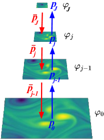
Figure 1: The renormalization group (illustrated in blue) computes the probability distributions $p_{j}(\varphi_{j})$ of images $\varphi_{j}$ at progressively larger scales $2^{j}$, with marginal integrations of high-frequency degrees of freedom, up to a maximum scale $2^{J}$. A hierarchic flow (illustrated in red) is a top-down inverse Markov chain which recovers $p$ from $p_{J}$ by estimating each transition probability $\bar{p}_{j}$ from $p_{j}$ to $p_{j-1}$. Difficulties arise when $\bar{p}_{j}$ is non-local, as in turbulent flows.

A hierarchic probability flow across scales is an inverse to Wilson renormalization group. If we represent high frequencies in wavelet bases then the transition kernels can be written as conditional probabilities of wavelet coefficients. Renormalizing wavelet coefficients is a strategy to control log-Sobolev constants of transition probabilities. For the $\varphi^{4}$ model of ferromagnetism at phase transition, it was shown in [marchand_wavelet_2022] that a renormalization in a wavelet basis eliminates the ”critical slowing down” of Langevin sampling algorithms [10.1093/oso/9780198834625.001.0001]. This is verified and analyzed for different types of wavelet bases in Section LABEL:sec:scal-pot-ene. The $\varphi^{4}$ scalar potential model has local spatial interactions. It is ”renormalizable,” which means that it can be approximated with a number of coupling parameters, which does not depend on the field dimension $d$, at all scales. This property does not apply to complex systems such as fluid turbulence, which have progressively more degrees of freedom as the dimension $d$ increases [Bohr_Jensen_Paladin_Vulpiani_1998]. To face this issue, we introduce hierarchic potential models, whose dimensions increase when the scale $2^{j}$ decreases. The hierarchy preserves a coupling flow equation, which relates the coupling parameters of energies from one scale to the next.

In physics and statistics, Gibbs energies of non-Gaussian probability distributions are often approximated with polynomials of degrees larger than $2$, typically $3$ or $4$ [landau2013statistical]. For a stationary field of dimension $d$, it involves $d^{2}$ or $d^{3}$ approximation terms, whose estimations have a large variance. Section LABEL:sec:scat-cov introduces interaction energy models of dimension $O(\log^{3}d)$, with robust multiscale approximations of high order polynomial energies. They are computed with a second wavelet transform, applied to the modulus of the first wavelet transform. It defines a second hierarchy, with a second scale parameter. The resulting scattering coefficients [mallatscat] capture long-range non-Gaussian interactions across space and scales [cheng2023scattering]. These interaction energy models provide a renormalization group representation of non-renormalizable systems, with $O(\log^{3}d)$ degrees of freedom, which increases slowly with the dimension $d$. Numerical applications are shown to estimate and sample Gibbs energy models of two-dimensional turbulent vorticity fields and dark matter density fields.

2 Probability Models, Estimation and Sampling

We denote by $\varphi\in{\mathbb{R}}^{d}$ a data vector of dimension $d$. We suppose that it has a probability density $p(\varphi)={\cal Z}^{-1}e^{-{U}(\varphi)}$ with respect to the Lebesgue measure, with a Gibbs energy $U$ which is twice differentiable. Our goal is to estimate an accurate model of $p$ from $m$ samples $\{\varphi^{(i)}\}_{i\leq m}$, and to generate new data by sampling this model. This section is a brief introduction to sampling of high-dimensional probabilities with Langevin diffusions, and to the estimation of parametric models by maximum likelihood and score matching.

2.1 Langevin Sampling and Log Sobolev Inequalities

If ${U}(\varphi)$ is known, one can sample $p$ with a Langevin dynamics, which is a Markov process that iteratively updates a field $\varphi_{t}$ with the stochastic differential equation

$$d\varphi_{t}=-\nabla_{\varphi}{U}(\varphi_{t})\,dt+\sqrt{2}\,dB_{t}\leavevmode\nobreak\ ,$$

where $B_{t}$ is a Brownian motion. It is a gradient descent on the energy, which is perturbed by the addition of a Gaussian white noise. Let $\varphi_{0}$ be a sample of a density $p_{0}$ at time $t=0$. At time $t$, $\varphi_{t}$ is a sample of a density $p_{t}$ which is guaranteed to converge to the density $p$ of Gibbs energy ${U}(\varphi)$ [Lelièvre_Stoltz_2016]. The unique invariant measure of this Markov chain is $p$. We can thus sample $p$ by running Langevin equation over samples of an initial measure $p_{0}$, for example Gaussian, but the convergence may be extremely slow.

The convergence of $p_{t}$ towards $p$ is defined with a KL divergence

$$KL(p_{t},p)=\int p_{t}(\varphi)\,\log\frac{p_{t}(\varphi)}{p(\varphi)}\,d\varphi\geq 0.$$

De Bruin identity [bauerschmidt2023stochastic] proves that

$$\frac{dKL(p_{t},p)}{dt}=-{\cal I}(p_{t},p),$$ (1)

where ${\cal I}$ is the relative Fisher information

$${\cal I}(q,p)=\int q(\varphi)\,\|\nabla_{\varphi}\log\frac{q(\varphi)}{p(\varphi)}\|^{2}\,d\varphi.$$

The exponential convergence of $p_{t}$ towards $p$ is guaranteed if $p$ satisfies a log-Sobolev inequality, which is recalled.

Definition 2.1.

The log-Sobolev constant $c(p)$ of $p$ is the smallest constant so that for any probability density $q$

$$KL(q,p)\leq c(p)\,{\cal I}(q,p).$$ (2)

Log-Sobolev constants relate entropy and gradients of smooth normalized functions $f(\varphi)$ in the functional space ${\bf L^{2}}(p\,d\varphi)$. Indeed, $f^{2}={q}/p$ satisfies $\|f\|_{2}=1$ in ${\bf L^{2}}(p\,d\varphi)$ because $\int q(\varphi)d\varphi=1$, and one can verify that the log-Sobolev inequality (2) is equivalent to

$$\int f^{2}(\varphi)\,\log f^{2}(\varphi)\,p(\varphi)d\varphi\leq 4\,c(p)\int\|\nabla f(\varphi)\|^{2}p(\varphi)d\varphi.$$ (3)

If $p$ is a normal Gaussian then $c(p)=1/2.$ The log-Sobolev constant gives an exponential rate of convergence of a Langevin diffusion. Indeed, inserting the log-Sobolev definition (2) in (1) proves that

$$KL(p_{t},p)\leq e^{{-t}/{c(p)}}KL(p_{0},p)\leavevmode\nobreak\ .$$ (4)

The time it takes for Langevin diffusions to reach a fixed precision is thus at most proportional to the log-Sobolev constant $c(p)$. The trouble is that $c(p)$ typically grows exponentially with the dimension $d$ of $\varphi$.

Upper bounds of the log-Sobolev constant can be computed in two cases [bauerschmidt2023stochastic]. Under independence conditions, if $\varphi=(\varphi_{k})_{k}$ and $p$ can be separated as a tensor product of densities $p(\varphi)=\prod_{k}p_{k}(\varphi_{k})$ then

$$c(p)=\max_{k}\big{(}c(p_{k})\big{)}_{k}.$$ (5)

In other words, the log-Sobolev constant of independent random variables is the maximum log-Sobolev constant of each variable. The second case, when ${U}$ is strongly convex, is the Bakry-Emery theorem [bakry2014analysis], which proves that

$$\forall\varphi\leavevmode\nobreak\ \leavevmode\nobreak\ ,\leavevmode\nobreak\ \leavevmode\nobreak\ \nabla^{2}_{\varphi}{U}(\varphi)\geq{\alpha}Id\leavevmode\nobreak\ \leavevmode\nobreak\ \Rightarrow\leavevmode\nobreak\ c(p)\leq\frac{1}{2{\alpha}}.$$ (6)

The maximum constant ${\alpha}$ satisfying this equality is the infimum over $\varphi$ of all eigenvalues of the Hessian matrices $\nabla^{2}_{\varphi}{U}(\varphi)$. The following proposition gives a lower bound of the log-Sobolev constant from the covariance of $p$.

Proposition 2.1.

Let $\mu_{\max}$ be the largest eigenvalue of the covariance of $p$. The log-Sobolev constant satisfies

$$c(p)\geq\mu_{\max}/2\leavevmode\nobreak\ .$$ (7)

This proposition is proved in Appendix LABEL:app:pointcarre. It comes from the inequality between log-Sobolev and Poincaré constants [ledoux2000geometry].

The Langevin diffusion is numerically calculated with an Euler-Maruyama discretization. If $\nabla_{\varphi}{U}(\varphi)$ is uniformly $L-$Lipschitz, then the discretization time step can be smaller or equal to $L^{-1}$ [vempala2022rapid]. Since $L$ is the supremum of all eigenvalues of the Hessians $\nabla^{2}_{\varphi}{U}(\varphi)$, it results from (4) that the number of Langevin diffusion steps to achieve a given precision is proportional to the log-Sobolev constant multiplied by this eigenvalue supremum. It is a normalization of the log-Sobolev constant, which specifies the computational complexity of the Langevin sampling algorithm.

Numerically, the convergence rate of a Langevin diffusion is estimated from the relaxation time $\tau$ of the auto-correlation

$$A(t)=\mathbb{E}$$ (8)