Next-to-leading-order electroweak correction to $H\to Z^{0}\gamma$

Abstract

Inspired by the recent observation of the Higgs boson radiative decay into $Z^{0}$ by ATLAS and CMS Collaborations, we investigate the next-to-leading-order (NLO) electroweak correction to this rare decay process in Standard Model (SM). Implementing the on-shell renormalization scheme, we find that the magnitude of the NLO electroweak correction may reach $7\%$ of the leading order (LO) prediction, much more significant than that of the NLO QCD correction, which is merely about $0.3\%$. After incorporating the ${\cal O}(\alpha)$ correction, the predicted partial width from various $\alpha$ schemes tend to converge to each other. Including both NLO electroweak and QCD corrections, we present the most accurate SM prediction for the branching fraction of this rare decay channel to be ${\cal B}_{\rm th}[H\to Z^{0}\gamma]=(1.55\pm 0.06)\times 10^{-3}$, considerably lower than the measured value ${\cal B}_{\rm exp}[H\to Z^{0}\gamma]=(3.4\pm 1.1)\times 10^{-3}$. Resolving this alarming discrepancy clearly calls for further theoretical investigations, and, more importantly, experimental efforts from HL-LHC and the prospective Higgs factories such as CEPC and FCC.

Introduction. The ground-breaking discovery of a 125 GeV boson at LHC in 2012 heralds a new era of particle physics ATLAS:2012yve ; CMS:2012qbp . After decade long experimental endeavours, the couplings between this new particle and $W$, $Z$, heavy fermions have been confirmed to be consistent with the Standard Model (SM) predictions, provided that this new boson is identified with the Higgs boson ATLAS:2016neq ; ATLAS:2022vkf ; CMS:2022dwd . Nevertheless, it is still important to test the SM predictions in some rare decay channels of Higgs boson, exemplified by $H\to Z^{0}\gamma$. As a loop-induced process, this decay channel serves a fruitful platform to look for the footprints of new particles predicted in many beyond Standard Model (BSM) scenarios.

Recently, the ATLAS and CMS Collaborations jointly reported the evidence of observing the rare decay $H\to Z^{0}\gamma$ ATLAS:2023yqk ; ATLAS:2020qcv ; CMS:2022ahq , and found $\mu_{Z\gamma}=2.2\pm 0.7$, with $\mu\equiv(\sigma{\cal B})_{\rm meas}/(\sigma{\cal B})_{\rm th}$ being a parameter to gauge how well the measurement conforms to the SM prediction. The measured branching fraction is ${\cal B}(H\to Z\gamma)=(3.4\pm 1.1)\times 10^{-3}$, more than twice larger than the SM prediction $(1.5\pm 0.1)\times 10^{-3}$ Djouadi:1997yw ; LHCHiggsCrossSectionWorkingGroup:2016ypw . This should be contrasted with a similar channel $H\to\gamma\gamma$ with $\mu_{\gamma\gamma}=1.10\pm 0.07$, which exhibits a satisfactory agreement between the measurement and the SM prediction. Recently there has appeared a flurry of work attempting to alleviate the discrepancy between experiment and theory for $H\to Z^{0}\gamma$, by invoking various BSM models Hong:2023mwr ; Panghal:2023iqd ; Buccioni:2023qnt ; Boto:2023bpg ; Cheung:2024kml ; He:2024sma .

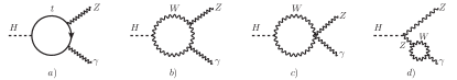
Figure 1: Some representative LO diagrams for $H\to Z^{0}\gamma$.

Needless to say, in order to ultimately resolve the discrepancy related to $H\to Z^{0}\gamma$, it is compulsive to first have a as precise as possible prediction in SM. At leading order (LO), the process $H\to Z^{0}\gamma$ is mediated via a heavy quark or a $W$ boson loop, as depicted in Fig. 1. The LO prediction has been available four decades ago Cahn:1978nz ; Bergstrom:1985hp . It turns out that the $W$-loop induced contribution dominates the $t$-loop induced one, while there exists a destructive interference between these two channels. The NLO QCD correction in numerical form has been known in early 90s Spira:1991tj , and its analytical form has also been available about one decade ago Gehrmann:2015dua ; Bonciani:2015eua . The QCD correction appears to be rather insignificant. This may be partly be understood by the fact that the gluons can only feel the top quark loop, which by itself only yields a small portion of the contribution with respect to the $W$ loop.

Therefore, the missing NLO electroweak correction is envisaged to constitute the major theoretical uncertainty for this decay channel, which has been estimated to reach $5\%$ level of the LO contribution LHCHiggsCrossSectionWorkingGroup:2016ypw . It is the goal of this work to conduct a complete investigation of the NLO electroweak correction to $H\to Z^{0}\gamma$.

Partial width from form factors. Let us express the amplitude for $H\to Z^{0}\gamma$ as $\mathcal{A}=T_{\mu\nu}\varepsilon^{\mu*}_{Z}(p_{1})\varepsilon^{\nu*}_{\gamma}(p_{2})$. By Lorentz invariance, $T_{\mu\nu}$ can be decomposed into the following most general tensor structures:

$$T^{\mu\nu} = p_{1}^{\mu}p_{1}^{\nu}T_{1}+p_{2}^{\mu}p_{2}^{\nu}T_{2}+p_{1}^{\mu}p_{2}^{\nu}T_{3}+p_{2}^{\mu}p_{1}^{\nu}T_{4}$$ (1)

$$+ p_{1}\cdot p_{2}g^{\mu\nu}T_{5}+\epsilon^{\mu\nu\alpha\beta}p_{1\alpha}p_{2\beta}T_{6},$$

where $p_{1}$ and $p_{2}$ signify the momenta of the outgoing $Z$ boson and photon, respectively, and $T_{i}$ ($i=1,\cdots 6$) signify six scalar form factors. The transversity condition $p_{1}\cdot\epsilon_{Z}=p_{2}\cdot\epsilon_{\gamma}=0$ implies that the terms entailing $T_{2}$ and $T_{3}$ do not contribute. Ward identity $p_{2\nu}T^{\mu\nu}=0$ implies that $T_{1}=0$ and $T_{4}=-T_{5}$. $T_{6}$ first starts at two-loop electroweak correction, which can thus be safely neglected as far as we concentrate on the NLO electroweak correction. Therefore only one independent form factor, $T_{5}=-T_{4}$, survives. In practice, it is convenient to introduce a new dimensionless form factor $\widetilde{T}_{5}$:

$$T_{5}=\frac{M_{H}^{2}}{M_{W}s_{W}(M_{H}^{2}-M_{Z}^{2})}\widetilde{T}_{5},$$ (2)

where $c_{W}\equiv\tfrac{M_{W}}{M_{Z}}$, and $s_{W}=\sqrt{1-c_{W}^{2}}$. The partial width then becomes

$$\Gamma(H\to Z^{0}\gamma)=\frac{1}{2M_{H}}\frac{1}{8\pi}\frac{2|{\bf p}_{1}|}{M_{H}}\frac{M_{H}^{4}}{2M_{W}^{2}s_{W}^{2}}|\widetilde{T}_{5}|^{2},$$ (3)

where the three-momentum of the $Z^{0}$ boson in the Higgs boson rest frame is $|{\bf p}_{1}|={(M_{H}^{2}-M_{Z}^{2})}/{2M_{H}}$. Our main task is to deduce $\widetilde{T}_{5}$ through NLO in $\alpha$.

Outline of calculation. Throughout this work we adopt the Feynman gauge and employ the dimensional regularization to regularize the potential UV divergence. We utilize the package FeynArts Hahn:2000kx to generate the Feynman diagrams and the corresponding amplitudes for $H\to Z^{0}\gamma$ through NLO in $\alpha$. This process entails approximately 50 diagrams at one-loop level, and more than $10^{4}$ diagrams at two-loop level. Some representative diagrams relevant to the NLO QCD and electroweak corrections are depicted in Fig. 2. The form factors $T_{4}$ and $T_{5}$ are extracted from the amplitude with the aid of the covariant projectors Bonciani:2015eua . We employ the packages FeynCalc Mertig:1990an and FormLink Feng:2012tk to perform Lorentz contraction and Dirac matrix trace. We use the packages Apart Feng:2012iq and FIRE Smirnov:2014hma for integration-by-part reduction. We end up with 8 one-loop master integrals (MIs) and over 700 two-loop MIs. The package AMFlow Liu:2017jxz ; Liu:2022mfb ; Liu:2022chg is invoked to evaluate all these MIs with high numerical accuracy.

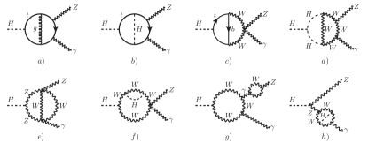
Figure 2: Some representative two-loop diagrams for $H\to Z^{0}\gamma$. $a)$ represents a sample diagram for NLO QCD correction, while $b)$-$h)$ represent sample diagrams for the NLO electroweak correction.

The on-shell renormalization scheme has been widely used in the field of electroweak radiative correction to tame the UV divergence Ross:1973fp ; Hollik:1988ii . The renormalized parameters are chosen to be those measured very precisely, such as Higgs boson mass, $W/Z$ masses, top quark mass, and QED coupling at Thomson limit. Having implemented the mass and charge renormalization ($e_{0}=Z_{e}e$), we find it convenient to stay with the bare field in the practical calculation. Following the LSZ reduction formula, we multiply the amputated amplitude of $H\to Z^{0}\gamma$ by the factor $\sqrt{Z_{H}Z_{ZZ}Z_{\gamma\gamma}}$, where the $Z_{H}$, $Z_{ZZ}$ and $Z_{\gamma\gamma}$ denote the field-strength renormalization constants associated with $H$, $Z^{0}$ and $\gamma$, respectively. These field strength renormalization constants can be inferred from the unrenormalized propagators to one loop accuracy, by identifying the residues in the on-shell limit.

It is worth mentioning that we have explicitly included those diagrams where $Z^{0}$ via a loop converts into a outgoing photon in the external leg, as depicted in Fig. 1$d)$ and Fig. 2$g)$, $h)$. Note it is not necessary in our treatment to include the contributions from the low-order diagrams multiplying the counterterms $\delta Z_{ZA}$ and $\delta Z_{AZ}$ characterizing the mixing between the $Z^{0}$ and $\gamma$ .

After carrying out the mass and charge renormalization, we finally end up with the UV-finite results for $T_{4}$ and $T_{5}$. We have confirmed the Ward identity requirement $T_{4}=-T_{5}$ holds at ${\cal O}(\alpha)$ level, which serves a nontrivial crosscheck.

Three different recipes about charge renormalization. Implementing the charge renormalization in electroweak theory is not unique, which leads to several popular variants in the on-shell renormalization scheme. In the so-called $\alpha(0)$ scheme, where the $\alpha$ is taking the Thomson-limit value, To one-loop order, $\delta Z_{e}$ is expressed as

$$\delta Z_{e}|_{\alpha(0)}={1\over 2}{\Pi^{\gamma\gamma}(0)}-{s_{W}\over c_{W}}{\Sigma^{\gamma Z}_{T}(0)\over M_{Z}^{2}},$$ (4)

where ${\Pi(s)}\equiv\Sigma_{T}^{\gamma\gamma}(s)/s$. The photon vacuum polarization is sensitive to the low-energy hadronic contribution, thereby an intrinsically non-perturbative quantity. Alternatively, one may rewrite $\delta{Z_{e}}$ in $\alpha(0)$ scheme as

$$\delta{Z_{e}}\big{|}_{\alpha(0)} = {1\over 2}\Delta{\alpha_{\rm had}^{(5)}}(M_{Z})+{1\over 2}{\rm Re}\,\Pi^{\gamma\gamma(5)}(M_{Z}^{2})$$ (5)

$$+ {1\over 2}\Pi^{\gamma\gamma}_{\rm rem}(0)-{s_{W}\over c_{W}}{\Sigma^{\gamma Z}_{T}(0)\over M_{Z}^{2}},$$

where $\Pi^{\gamma\gamma(5)}(M_{Z}^{2})$ is the photon vacuum polarization from five massless quarks at momentum transfer $M_{Z}^{2}$. $\Delta{\alpha_{\rm had}^{(5)}}(M_{Z})$, being a non-perturbative parameter, absorbs the hadronic contribution to photon vacuum polarization, which can be determined from the measured $R$ values in low-energy $e^{+}e^{-}$ experiments. $\Pi^{\gamma\gamma}_{\rm rem}(0)$ represents the vacuum polarization from the $W$ boson, charged leptons and top quark at zero momentum transfer. Note all these terms except $\Delta{\alpha_{\rm had}^{(5)}}(M_{Z})$ can be computed reliably in perturbation theory.

Two other popular variants of the on-shell renormalization scheme are the $\alpha(M_{Z})$ and $G_{\mu}$ schemes. The corresponding charge renormalization constant can be converted from (4) by $\delta{Z_{e}}\big{|}_{\alpha(M_{Z})}=\delta{Z_{e}}\big{|}_{\alpha(0)}-{1\over 2}\Delta\alpha(M_{Z})$, and $\delta Z_{e}|_{G_{\mu}}=\delta Z_{e}|_{\alpha(0)}-{1\over 2}\Delta r$, respectively. $\Delta\alpha(M_{Z})=\Pi^{\gamma\gamma}_{f\neq t}(0)-{\rm Re}\,\Pi^{\gamma\gamma}_{f\neq t}(M_{Z}^{2})$, and the expression for the oblique parameter $\Delta r$ can be found in Denner:1991kt . The QED coupling constant in the $\alpha(M_{Z})$ and $G_{\mu}$ schemes read

$$\alpha\left(M_{Z}\right)=\frac{\alpha(0)}{1-\Delta\alpha\left(M_{Z}\right)},$$ (6a)

$$\alpha_{G_{\mu}}=\frac{\sqrt{2}}{\pi}G_{\mu}M_{W}^{2}\left(1-\frac{M_{W}^{2}}{M_{Z}^{2}}\right).$$ (6b)

In contrast to the $\alpha(0)$ scheme, these two sub-schemes effectively resum some universal large (non-)logarithmic terms arising from the light fermions and top quark loop.

Numerical predictions. To make concrete predictions, we adopt the following values for the masses of various particles Workman:2022ynf :

$$M_{H}=125.25\>{\rm GeV},\quad M_{Z}=91.1876\>{\rm GeV},$$

$$M_{W}=80.377\>{\rm GeV},\quad m_{t}=172.69\>{\rm GeV},$$

$$m_{e}=0.5109989\>{\rm MeV},\quad m_{\mu}=105.65837\>{\rm MeV},$$

$$m_{\tau}=1.77686\>{\rm GeV}.$$ (7)

The masses of the charged leptons are retained only for the purpose of computing $Z_{e}$. In all other situations, we only keep the top quark massive and set the remaining five quarks and all charged leptons to be massless.

We adopt the following values of couplings: $\alpha(0)=1/137.035999$, $G_{\mu}=1.1663787\times 10^{-5}~{}{\rm GeV}^{-2}$ and $\Delta\alpha_{\rm had}^{(5)}(M_{Z})=0.02764$ Workman:2022ynf . We also take $\alpha(M_{Z})=1/128.877$ from Refs. Eidelman:1995ny ; Steinhauser:1998rq . With the aid of (6b) one obtains $\alpha_{G_{\mu}}=1/132.168$.

The current measured full width of the Higgs is subject to large uncertainty, $\Gamma_{H}=3.2^{+2.4}_{-1.7}$ MeV Workman:2022ynf . When predicting the branching fraction, we choose to use the much more precise prediction. Thus, it is more convenient to use the theoretically predicted value, $\Gamma_{H}=4.07^{+4.0\%}_{-3.9\%}$ MeV Workman:2022ynf ; LHCHiggsCrossSectionWorkingGroup:2016ypw .

	$\alpha$ assignment at LO	$\Gamma^{\rm LO}$	$\Gamma^{\mathcal{O}(\alpha)}$	$\Gamma^{\mathcal{O}(\alpha_{s})}$	$\Gamma^{\rm Sum}$	${\cal B}(\times 10^{-3})$
$\alpha(0)$ scheme	$\alpha(0)^{3}$	$5.920$	$0.439$	$0.018$	$6.378$	$1.57\pm 0.06$
$\alpha(M_{Z})$ scheme	$\alpha(0)\alpha(M_{Z})^{2}$	$6.694$	$-0.465$	$0.021$	$6.249$	$1.54\pm 0.06$
$G_{\mu}$ scheme	$\alpha(0)\alpha_{G_{\mu}}^{2}$	$6.364$	$-0.048$	$0.020$	$6.336$	$1.56\pm 0.06$
Democratic scheme	$\alpha(0)\alpha(M_{Z})\alpha_{G_{\mu}}$	$6.528$	$-0.249$	$0.020$	$6.299$	$1.55\pm 0.06$

Table 1: Predicted values of the partial width (in units of keV) for $H\to Z^{0}\gamma$ in various $\alpha$ schemes, at various levels of perturbative accuracy. $\Gamma^{\rm LO}$ represents the LO prediction to the decay width. The contributions from the NLO electroweak and QCD corrections are denoted by $\Gamma^{\mathcal{O}(\alpha)}$ and $\Gamma^{\mathcal{O}(\alpha_{s})}$, respectively. We have taken the strong coupling constant $\alpha_{s}(M_{H})=0.113$. $\Gamma^{\rm Sum}$ is obtained by summing the LO contribution together with $\mathcal{O}(\alpha)$ and $\mathcal{O}(\alpha_{s})$ corrections, and the rightmost column is the branching fraction obtained via dividing $\Gamma^{\rm Sum}$ by the full Higgs width, $\Gamma_{H}=4.07^{+4.0\%}_{-3.9\%}$ MeV.

In Appendix A we present the numerical results of the form factor $\widetilde{T}_{5}$ at NLO accuracy in different $\alpha$ schemes. Plugging into (3), we are able to present the predictions for the partial width in various $\alpha$ schemes. It may look natural to take the QED coupling constant at the vertex attached to the outgoing photon as $\alpha(0)$. For the electromagnetic coupling constant that appears elsewhere, one has some freedom to choose different $\alpha$ scheme. In Table 1 we enumerate our predictions for $\Gamma(H\to Z^{0}\gamma)$ (in units of keV) based on four different $\alpha$ schemes at various levels of perturbative accuracy.

As can be seen from Table 1, we confirm that the NLO QCD correction is positive but tiny, which constitutes only $0.3\%$ of the LO partial width Bonciani:2015eua . We also notice that, the NLO electroweak corrections is positive in the $\alpha(0)$ scheme, while negative in other three schemes. In addition, the ${\cal O}(\alpha)$ corrections appear to be sizable in magnitude in both the $\alpha(0)$ and $\alpha(M_{Z})$ schemes, which may approach approximately $7\%$ of the LO prediction. In contrast, the $G_{\mu}$ scheme as well as the Democratic scheme yield a relatively modest ${\cal O}(\alpha)$ correction. Note the LO predictions of the partial width from four different $\alpha$ scheme are scattered in a wide range, from $5.920$ keV to $6.694$ keV. Interestingly, after including the NLO electroweak correction, the scheme dependence becomes substantially reduced, with the relative uncertainties among different schemes less than $2\%$. Taking the predictions from various $\alpha$ schemes as an estimation of the theoretical uncertainty, we then obtain the most accurate SM prediction to be ${\cal B}[H\to Z^{0}\gamma]=(1.55\pm 0.06)\times 10^{-3}$. Note the error in the branching fraction mainly stem from the uncertainty associated with the full width the of the Higgs boson .

It is evident that the most accurate SM prediction for the branching fraction is significantly lower than the measured value, ${\cal B}_{\rm exp}[H\to Z^{0}\gamma]=(3.4\pm 1.1)\times 10^{-3}$ ATLAS:2023yqk . It may be too early to claim that some sort of the BSM physics must be invoked to resolve this discrepancy. More accurate measurements from HL-LHC, and the prospective Higgs factories such as CEPC and FCC, will play a crucial role to clear the smoke.

Summary. In this work we have calculated the NLO electroweak correction to the rare decay process $H\to Z^{0}\gamma$ within the on-shell renormalization scheme. To assess the theoretical uncertainty, we present the predictions of the partial width and the branching fraction using several different $\alpha$ schemes. In contrast to the tiny NLO QCD correction, the magnitude of the NLO electroweak correction turns out to become sizable, reaching $7\%$ of the LO result in both the $\alpha(0)$ and $\alpha(M_{Z})$ schemes. After including the ${\cal O}(\alpha)$ correction, the predictions from various $\alpha$ schemes tend to converge to each other, which indicates that incorporating the NLO electroweak correction has significantly stabilized the SM prediction. Our most accurate prediction is then ${\cal B}[H\to Z^{0}\gamma]=(1.55\pm 0.06)\times 10^{-3}$, with the uncertainty predominantly stemming from the error of the full width of Higgs. The relative error from varying the $\alpha$ schemes is less than $2\%$. Although this most accurate SM prediction is significantly lower than the measured value, it might be premature to claim that one has to invoke the new physics to resolve this discrepancy. Likely the problem mainly lies on the experimental side. Improved measurement of this rare decay process at HL-LHC, and independent measurements at the prospective Higgs factories such as the CEPC and the FCC, are crucial.

Note added. While we were finalizing this work, a preprint by Chen, Chen, Qiao and Zhu has recently appeared Chen:2024vyn . Our results for the $\alpha({M_{Z}})$ and $G_{\mu}$ schemes are compatible with their mixed 1 and mixed 2 schemes, provided that the same input parameters are used. However, our result for the $\alpha(0)$ scheme slightly differs from theirs, probably due to the different treatment of the light quark contribution to $Z_{e}$.

Appendix A The expressions of $\widetilde{T}_{5}$ from four different $\alpha$ schemes

As aforementioned, there are some freedoms in the on-shell renormalization scheme to handle the charge renormalization. In this appendix, we present the expressions of the form factor $\widetilde{T}_{5}$ in four different schemes, which differ in choosing the values of the QED coupling constant. Throughout this work we always retain the QED coupling associated with the photon emission vertex to be $\alpha(0)$. Plugging these equations into (3), we then obtain the predicted partial widths associated in each scheme, as enumerated in Table 1.

A.1 $\alpha(0)$ scheme

In this scheme, all the QED couplings in three vertices of the LO diagrams in Fig. 1 are chosen to be $\alpha(0)$, i.e., the fine structure constant in the Thomson limit. After including both ${\cal O}(\alpha)$ and ${\cal O}(\alpha_{s})$ corrections, the form factor $\widetilde{T}_{5}$ reads

$$\widetilde{T}_{5}=1.546\,\alpha^{3/2}(0)\bigg{[}1+\Delta{\alpha_{\rm had}^{(5)}}(M_{Z})+4.070\;\frac{\alpha(0)}{\pi}$$ (8)

$$\quad\quad\quad\quad\quad\quad+0.043\;\frac{\alpha_{s}}{\pi}\bigg{]},$$

which depends on the light charged leptons but not on light quarks (whose effect has been included in $\Delta{\alpha_{\rm had}^{(5)}}(M_{Z})$). As can be clearly seen, the prefactor accompanying $\alpha(0)$ is about two orders-of-magnitude greater than that accompanying $\alpha_{s}$, which explains why the electroweak correction is much more important than the QCD correction.

A.2 $\alpha(M_{Z})$ scheme

In this scheme, we choose the QED coupling constants associated with two vertices other than the photon emission vertex in Fig. 1 to be $\alpha(M_{Z})$. Making the following replacement in (8):

$$\alpha(0) \to \alpha(M_{Z})\bigg{[}1-\Delta{\alpha_{\rm had}^{(5)}}(M_{Z})-\Delta\alpha_{\ell}(M_{Z})\bigg{]}$$ (9)

$$= \alpha(M_{Z})\bigg{[}1-0.02764-18.132\,\frac{\alpha(M_{Z})}{\pi}\bigg{]},\phantom{xx}$$

where $\Delta\alpha_{\ell}(M_{Z})=\Pi^{\gamma\gamma}_{f=e,\mu,\tau}(0)-{\rm Re}\,\Pi^{\gamma\gamma}_{f=e,\mu,\tau}(M_{Z})$, we then obtain

$$\widetilde{T}_{5}=1.546\,\alpha^{1/2}(0)\alpha(M_{Z})\bigg{[}1-14.062\;\frac{\alpha(M_{Z})}{\pi}$$ (10)

$$\quad\quad\quad\quad\quad\quad+0.043\;\frac{\alpha_{s}}{\pi}\bigg{]}.$$

Note $\widetilde{T}_{5}$ is insensitive of the mass of all light fermions.

A.3 $G_{\mu}$ scheme

In this scheme, we choose the QED coupling constants affiliated with two vertices other than the photon emission vertex in Fig. 1 to be $\alpha_{G_{\mu}}$. Making the following substitution in (8):

$$\alpha(0) \to \alpha_{G_{\mu}}\bigg{[}1-\Delta{\alpha_{\rm had}^{(5)}}(M_{Z})+\Delta\alpha_{lq}(M_{Z})-\Delta r\bigg{]}$$ (11)

$$= \alpha_{G_{\mu}}\bigg{[}1-0.02764-5.635\,\frac{\alpha_{G_{\mu}}}{\pi}\bigg{]},\phantom{xx}$$

with $\Delta\alpha_{lq}(M_{Z})=\Pi^{\gamma\gamma}_{f=u,d,s,c,b}(0)-{\rm Re}\,\Pi^{\gamma\gamma}_{f=u,d,s,c,b}(M_{Z})$, we obtain

$$\widetilde{T}_{5}=1.546\,\alpha^{1/2}(0)\alpha_{G_{\mu}}\bigg{[}1-1.565\;\frac{\alpha_{G_{\mu}}}{\pi}$$ (12)

$$\quad\quad\quad\quad\quad\quad+0.043\;\frac{\alpha_{s}}{\pi}\bigg{]}.$$

As in $\alpha(M_{Z})$ scheme, $\widetilde{T}_{5}$ in $G_{\mu}$ scheme is also independent of the masses of all light fermions.

A.4 Democratic scheme

In the Democratic scheme, we choose the QED couplings affiliated with three vertices in Fig. 1 to be $\alpha_{G_{\mu}}$, $\alpha(M_{Z})$, and $\alpha(0)$, respectively. By plugging (9) and (11) into (8), we obtain

$$\widetilde{T}_{5}=1.546\,\alpha^{1/2}(0)\alpha^{1/2}(M_{Z})\alpha_{G_{\mu}}^{1/2}\bigg{[}1-7.814\times$$ (13)

$$\quad\quad\quad\quad\quad\quad\;\frac{\alpha^{1/2}(M_{Z})\alpha_{G_{\mu}}^{1/2}}{\pi}+0.043\;\frac{\alpha_{s}}{\pi}\bigg{]}.$$

References

- (1) G. Aad et al. [ATLAS], Phys. Lett. B 716, 1-29 (2012) doi:10.1016/j.physletb.2012.08.020 [arXiv:1207.7214 [hep-ex]].
- (2) S. Chatrchyan et al. [CMS], Phys. Lett. B 716, 30-61 (2012) doi:10.1016/j.physletb.2012.08.021 [arXiv:1207.7235 [hep-ex]].
- (3) G. Aad et al. [ATLAS and CMS], JHEP 08, 045 (2016) doi:10.1007/JHEP08(2016)045 [arXiv:1606.02266 [hep-ex]].
- (4) G. Aad et al. [ATLAS], Nature 607, no.7917, 52-59 (2022) [erratum: Nature 612, no.7941, E24 (2022)] doi:10.1038/s41586-022-04893-w [arXiv:2207.00092 [hep-ex]].
- (5) A. Tumasyan et al. [CMS], Nature 607, no.7917, 60-68 (2022) [erratum: Nature 623, no.7985, E4 (2023)] doi:10.1038/s41586-022-04892-x [arXiv:2207.00043 [hep-ex]].
- (6) G. Aad et al. [ATLAS and CMS], Phys. Rev. Lett. 132, no.2, 021803 (2024) doi:10.1103/PhysRevLett.132.021803 [arXiv:2309.03501 [hep-ex]].
- (7) G. Aad et al. [ATLAS], Phys. Lett. B 809, 135754 (2020) doi:10.1016/j.physletb.2020.135754 [arXiv:2005.05382 [hep-ex]].
- (8) A. Tumasyan et al. [CMS], JHEP 05, 233 (2023) doi:10.1007/JHEP05(2023)233 [arXiv:2204.12945 [hep-ex]].
- (9) A. Djouadi, J. Kalinowski and M. Spira, Comput. Phys. Commun. 108, 56-74 (1998) doi:10.1016/S0010-4655(97)00123-9 [arXiv:hep-ph/9704448 [hep-ph]].
- (10) D. de Florian et al. [LHC Higgs Cross Section Working Group], doi:10.23731/CYRM-2017-002 [arXiv:1610.07922 [hep-ph]].
- (11) T. T. Hong, V. K. Le, L. T. T. Phuong, N. C. Hoi, N. T. K. Ngan and N. H. T. Nha, PTEP 2024, no.3, 033B04 (2024) doi:10.1093/ptep/ptae029 [arXiv:2312.11045 [hep-ph]].
- (12) S. Panghal and B. Mukhopadhyaya, [arXiv:2310.04136 [hep-ph]].
- (13) F. Buccioni, F. Devoto, A. Djouadi, J. Ellis, J. Quevillon and L. Tancredi, Phys. Lett. B 851, 138596 (2024) doi:10.1016/j.physletb.2024.138596 [arXiv:2312.12384 [hep-ph]].
- (14) R. Boto, D. Das, J. C. Romao, I. Saha and J. P. Silva, Phys. Rev. D 109, no.9, 095002 (2024) doi:10.1103/PhysRevD.109.095002 [arXiv:2312.13050 [hep-ph]].
- (15) K. Cheung and C. J. Ouseph, [arXiv:2402.05678 [hep-ph]].
- (16) X. G. He, Z. L. Huang, M. W. Li and C. W. Liu, [arXiv:2402.08190 [hep-ph]].
- (17) R. N. Cahn, M. S. Chanowitz and N. Fleishon, Phys. Lett. B 82, 113-116 (1979) doi:10.1016/0370-2693(79)90438-6
- (18) L. Bergstrom and G. Hulth, Nucl. Phys. B 259, 137-155 (1985) [erratum: Nucl. Phys. B 276, 744-744 (1986)] doi:10.1016/0550-3213(85)90302-5
- (19) M. Spira, A. Djouadi and P. M. Zerwas, Phys. Lett. B 276, 350-353 (1992) doi:10.1016/0370-2693(92)90331-W
- (20) T. Gehrmann, S. Guns and D. Kara, JHEP 09, 038 (2015) doi:10.1007/JHEP09(2015)038 [arXiv:1505.00561 [hep-ph]].
- (21) R. Bonciani, V. Del Duca, H. Frellesvig, J. M. Henn, F. Moriello and V. A. Smirnov, JHEP 08, 108 (2015) doi:10.1007/JHEP08(2015)108 [arXiv:1505.00567 [hep-ph]].
- (22) T. Hahn, Comput. Phys. Commun. 140, 418-431 (2001) doi:10.1016/S0010-4655(01)00290-9 [arXiv:hep-ph/0012260 [hep-ph]].
- (23) R. Mertig, M. Bohm and A. Denner, Comput. Phys. Commun. 64, 345-359 (1991) doi:10.1016/0010-4655(91)90130-D
- (24) F. Feng and R. Mertig, [arXiv:1212.3522 [hep-ph]].
- (25) F. Feng, Comput. Phys. Commun. 183, 2158-2164 (2012) doi:10.1016/j.cpc.2012.03.025 [arXiv:1204.2314 [hep-ph]].
- (26) A. V. Smirnov, Comput. Phys. Commun. 189, 182-191 (2015) doi:10.1016/j.cpc.2014.11.024 [arXiv:1408.2372 [hep-ph]].
- (27) X. Liu, Y. Q. Ma and C. Y. Wang, Phys. Lett. B 779, 353-357 (2018) doi:10.1016/j.physletb.2018.02.026 [arXiv:1711.09572 [hep-ph]].
- (28) Z. F. Liu and Y. Q. Ma, Phys. Rev. Lett. 129, no.22, 222001 (2022) doi:10.1103/PhysRevLett.129.222001 [arXiv:2201.11637 [hep-ph]].
- (29) X. Liu and Y. Q. Ma, Comput. Phys. Commun. 283, 108565 (2023) doi:10.1016/j.cpc.2022.108565 [arXiv:2201.11669 [hep-ph]].
- (30) D. A. Ross and J. C. Taylor, Nucl. Phys. B 51, 125-144 (1973) [erratum: Nucl. Phys. B 58, 643-643 (1973)] doi:10.1016/0550-3213(73)90505-1
- (31) W. F. L. Hollik, Fortsch. Phys. 38, 165-260 (1990) doi:10.1002/prop.2190380302
- (32) A. Denner, Fortsch. Phys. 41, 307-420 (1993) doi:10.1002/prop.2190410402 [arXiv:0709.1075 [hep-ph]].
- (33) R. L. Workman et al. [Particle Data Group], PTEP 2022, 083C01 (2022) doi:10.1093/ptep/ptac097
- (34) S. Eidelman and F. Jegerlehner, Z. Phys. C 67, 585-602 (1995) doi:10.1007/BF01553984 [arXiv:hep-ph/9502298 [hep-ph]].
- (35) M. Steinhauser, Phys. Lett. B 429, 158-161 (1998) doi:10.1016/S0370-2693(98)00503-6 [arXiv:hep-ph/9803313 [hep-ph]].
- (36) D. Binosi, J. Collins, C. Kaufhold and L. Theussl, Comput. Phys. Commun. 180, 1709-1715 (2009) doi:10.1016/j.cpc.2009.02.020 [arXiv:0811.4113 [hep-ph]].
- (37) Z. Q. Chen, L. B. Chen, C. F. Qiao and R. Zhu, [arXiv:2404.11441 [hep-ph]].