Polynomial lower bound on the effective resistance for the one-dimensional critical long-range percolation
Abstract.
In this work, we study the critical long-range percolation on , where an edge connects and independently with probability for some fixed . Viewing this as a random electric network where each edge has a unit conductance, we show that with high probability the effective resistances from the origin 0 to and from the interval to (conditioned on no edge joining and ) both have a polynomial lower bound in . Our bound holds for all and thus rules out a potential phase transition (around ) which seemed to be a reasonable possibility.
Keywords: Long-range percolation, effective resistance, polynomial lower bound
MSC 2020: 60K35, 82B27, 82B43
1. Introduction
Consider the critical long-range percolation (LRP) on , where edges with (i.e. and are nearest neighbors) occur independently with probability , while edges with (which we refer to as long edges in what follows) occur independently with probability
| (1.1) |
Here, is a parameter of this LRP model. We also call this model as a -LRP model, and denote for the edge set. Additionally, for ease of notation, we will also use to denote edges, that is, implies . Note that we chose the expression (1.1) for the connecting probability since it has a strong scaling invariance property and is thus a convenient choice especially when studying scaling limits. That being said, it would be clear that our proof extends to the case when the connecting probability is within a multiplicative constant of .
In this study, we focus on the particular case for , where the connectivity, thus the existence of the infinite cluster, is trivial. Placing a unit conductance on each edge, we may then view this LRP model as a random electric network on . Our goal is to study the effective resistance (of the -LRP), which we now define. Let be a function defined on . We call a flow on the -LRP model if it satisfies
for all . So the net flow out of a point is . Moreover, given two finite disjoint subsets , we say is a unit flow from to if it is a flow satisfying
Note that the condition above implies . The effective resistance between disjoint subsets is then defined as
| (1.2) |
where the first infimum is taken over all finite subsets and . In particular, when is a singleton, we denote as .
Our main result establishes polynomial lower bounds on effective resistances, as detailed in the following theorem. For any subset , we denote by .
Theorem 1.1.
For any , there exists a constant (depending only on ) such that the following holds. For any , there exists a constant (depending only on and ) such that for all ,
| (1.3) |
and
| (1.4) |
1.1. Related work
Electric networks are commonly associated with reversible Markov chains, providing a sophisticated and efficient method for understanding properties of these chains [13, 18]. An essential measurement in electric network theory is the effective resistance, which plays a crucial role in evaluating the conductivity of the electric network. Effective resistances are closely related to various aspects of random walks on networks, including recurrence/transience, heat kernels and mixing times, see e.g. [1, 17, 15].
The study of effective resistances for LRP on has sparked great interests, as this measurement is not only an intriguing intrinsic property of the underlying random graph but also provides effective tools for studying random walks on this model. Specifically, consider the sequence , where and for all such that . Assume that
for some . The LRP on , introduced by [21, 22], is defined by edges occurring independently with probability .
We first review progress on effective resistances as well as behavior for random walks on non-critical (i.e. ) LRP models. In [16] the authors employed methods to estimate volumes and effective resistances from points to boxes, obtaining the corresponding heat kernel estimates for the case where and . In fact, the authors showed this in a more general random media setting. In [19], the author derived up-to-constant estimates for the box-to-box resistances for as well as for and . For random walks on infinite clusters of these LRP models, when , it was shown in [12] (for ) and [6] (for and ) that the random walk on the infinite cluster converges to an -stable process with . In the case where and , it was also shown in [12] that the random walk converges to a Brownian motion. It is worth mentioning that [7] studied the quenched invariance principle for random walks on LRP graphs with for all . According to [7, Problem 2.9], it seems that it remains a challenge to establish scaling limits of random walks on the LRP models with and . There are also numerous related results regarding the heat kernel, mixing time and local central limit theorem of the random walk, see e.g. [4, 11, 9, 10].
There are relatively few results for effective resistances and random walks on the critical LRP model for (note that in [19] resistance bounds are obtained in the critical case for ). The author of [5] established recurrence for the random walk in the case of for , by showing that the effective resistance from the origin to diverges as . This was then extended in [3] to more general LRP models with weight distribution satisfying some moment assumptions. In addition, bounds on box-to-box resistances were provided in [19] for , including a constant lower bound for . Despite these progresses, it seems a challenge to determine the divergence rate of the effective resistance. In fact, from our conversations with colleagues, it seems there is a folklore debate on whether for and the effective resistance grows polynomially for all or has a phase transition at . Our contribution in this work confirms the former scenario.
1.2. Outline of the proof of Theorem 1.1
Since the main ideas for proving (1.3) and (1.4) in Theorem 1.1 are essentially same, we mainly offer an overview for the proof of (1.3). To begin with, let us fix a sufficiently large and recall that the effective resistance is defined in (1.2) with and . Our objective is to establish a polynomial lower bound for the effective resistance .
When , intuitively there are relatively few long edges. This actually allows for a straightforward proof of a polynomial lower bound on by finding a sufficient number of cut-edges. Here, an edge is a cut-edge (and in general a set is a cut-set) if 0 is disconnected from after its removal. To be more specific, for , define
A simple calculation reveals that , leading to
which then (together with a second moment computation) implies a polynomial lower bound on the resistance. However, as increases, the number of long edges also increases, rendering the method of identifying cut-edges ineffective in providing a satisfactory lower bound.
In addition, as mentioned in Subsection 1.1, [19] established a constant lower bound for the effective resistance associated with our -LRP models. Indeed, the author showed the probability of the resistance being less than a certain constant is very low by choosing a specific test function in the dual variational formula of (1.2). However, obtaining a polynomial lower bound for the resistance through this method seems to be quite challenging, as a priori we have no information about the form of the function that achieves the infimum in the dual of (1.2). A diverging lower bound was shown in [5] via constructing a collection of disjoint cut-sets, although the bound diverges rather slowly. In fact, the method of [5] can be seen as an application of multi-scale analysis, although the contribution obtained from each scale is barely large enough to obtain a diverging lower bound. The key contribution of our work, as we elaborate in what follows, is to employ a novel framework of multi-scale analysis.
The main idea of our approach for multi-scale analysis is to provide a lower bound for the effective resistance by combining the total energy generated by flows in (1.2) passing through “good” subintervals of different scales within . The novelty of our multi-scale analysis is largely captured by the application of the analysis fact that
| (1.5) |
for all and some constants and (depending only on and ). Here , and is the -quantile of the “effective resistance” defined in (1.9) below. The key challenge of this work is to prove the recursive formula on the left-hand side of (1.5), and one difficulty is that we have to simultaneously control all unit flows. To this end, we partition the region near points where the flow enters the interval into intervals of length for . Then we search for “cut-intervals” at each step with layers. Here a cut-interval essentially plays the role of a cut-set, and roughly speaking it means that any unit flow from to must pass through the cut-interval (i.e., the flow must enter and then exit from the cut-interval). In our rigorous proof, the notion of cut-interval will be replaced by Definition 2.1. In addition, we will show that a significant fraction of cut-intervals will be very good, in the sense that when the flow passes through these intervals it generates a significant amount of energy (resulting in a significant contribution to effective resistances). By using this and suitably selecting associated parameters, we can establish the left-hand side of (1.5), as incorporated in Proposition 3.11.
Now, let us provide a slightly more detailed overview of the proof of (1.3) in Theorem 1.1. By a simple first moment computation, it is clear that with probability 1 there are only finitely many edges joining and . This implies that unit flows from 0 to are well-defined, since they can be viewed as unit flows from to the finite set
Now let be a unit flow from 0 to attaining the infimum in (1.2). Then, we can see that the flow emanates from 0 (with an outflow of ) and ultimately flows into (with an inflow of ). As a result, the flow must pass through intervals or (unless 0 is directly connected to , which is unlikely). So let us define as the portion of flow that passes through the interval and then flow into . Similarly, we define by replacing with in the definition of . We also let
| (1.6) |
represent amounts of flows exiting from intervals and , respectively. It is clear that . Define
| (1.7) | ||||
as the effective resistance generated by unit flows from to , passing through the interval . Similarly, denote as the effective resistance generated by unit flows from to , passing through the interval . Then we can deduce that
| (1.8) |
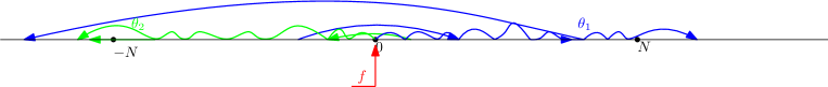
(See Figure 1 for an illustration). Note that and have the same distribution. Consequently, it suffices to prove that has a polynomial lower bound with high probability.
Furthermore, for the sake of convenience in employing an iterative approach for estimating resistances, we lower-bound via the resistance generated by unit flows from to passing through the interval , which is defined as
| (1.9) | ||||
(See Subsection 4.1 for more details). In conclusion, our primary focus is to establish a polynomial lower bound for the resistance as incorporated in Theorem 3.1.
To prove Theorem 3.1, we first introduce the concept of good pairs of intervals. Roughly speaking, for any and , we say the pair of intervals is good if any path originating from to must pass through either or (see Definition 2.1). Essentially, we may consider good pairs of intervals as some kind of “cut-intervals”. Hence, when the flow exits from , it must pass through at least one of these two intervals, generating a certain amount of energy. We will employ the Firework process theory (see e.g. [14]) by viewing coverage of long edges over intervals as the propagation in the Firework process, to obtain some estimates for the distribution of the number of intervals that can be covered at a time (see Lemma 2.4). The definition of an interval covered by long edges will be provided in (2.1) below. From this and a general Chernoff-Hoeffding bound, we can show that for a fixed , with high probability there exist a sufficient number of good pairs of intervals at various scales around it (see Proposition 2.2).
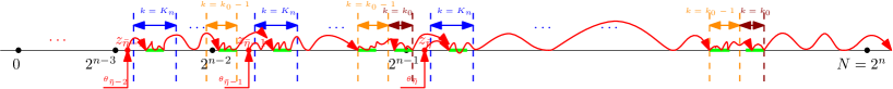
We next consider the area surrounding points where the unit flow (from to enters . We segment such area into intervals of length for , which we will refer to as the -th layer intervals. Then we search for good pairs of intervals at each step with layers and show that with high probability we can find enough good pairs of intervals in many layers (see Figure 5). Note that the here is in correspondence with in the subscript in (1.5) and is also responsible for the factor of in the denominator there. Therefore, when the flow passes through those good intervals, it will provide sufficiently large energies (i.e. effective resistances). This implies an effective lower bound for the resistance (see Lemma 3.13). Then we can establish a recursive formula for quantiles of the resistance (see Proposition 3.11). From this we can obtain a polynomial lower bound in for the resistance as in Theorem 3.1. We re-iterate that one difficulty is that we have to simultaneously control all unit flows. To achieve this, we show that good pairs of intervals found above through multi-scale analysis are essentially cut-sets, so all unit flows must pass through these intervals and then generate enough energy. This is incorporated in Section 3.
Notational conventions. We denote . For , we define . When we refer to an interval , it always implies that . For any two disjoint sets , let be a flow from to , we write for its amount, that is,
| (1.10) |
For example, if is a unit flow, then . In addition, for any two sets , we recall .
Throughout the paper, we use to denote positive constants, whose values are the same within each section but may vary from section to section.
2. Good intervals and associated estimates
For and , denote by and the intervals and , respectively.
Definition 2.1.
We say the pair of intervals is good if
-
(1)
and are not directly connected by any long edge;
-
(2)
and are not directly connected by any long edge.

In the following, we aim to provide a large deviation estimate for the number of good pairs of intervals. To do this, we only need to consider the case where due to the translation invariance of our model. For simplicity, we denote as in this case. We now define a sequence of Bernoulli random variables as
Proposition 2.2.
For any , there exists a constant (depending only on ) such that for all , we have
To prove Proposition 2.2, we need some preparations.
Lemma 2.3.
There is a constant (depending only on ) such that the following holds. For any and any in the ascending order, let
Then .
To prove Lemma 2.3, we will review the Firework process (see e.g. [14]) and view coverage of long edges over intervals as the propagation in the Firework process. For that, we fix and being a set in the ascending order.
For , let represent the minimum number of such that there exists at least one long edge within
where (see Figure 3 for an illustration). It is worth emphasizing that are independent from the independence of edges in our model. We say the pair of intervals is covered by long edges if there exists at least one long edge within
| (2.1) |
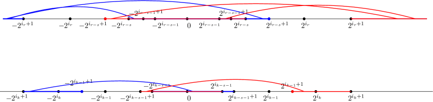
For the distribution of , we have the following property.
Lemma 2.4.
For and in the ascending order, we have
for all and .
Proof.
It follows from the definition of that for each and each ,
where the last inequality is from . ∎
We let and for , we inductively define
| (2.2) |
The above definition in fact corresponds to a “spreading” procedure of the edge set for the LRP model, where in the -th step we explore long edges in
| (2.3) |
to determine if the element is in . That is, if the edge set in (2.3) is non-empty, then . We see that (namely, the pair of intervals is newly covered at the -th step) if it was not covered by the edge set
but covered by the edge set in (2.3). The “spreading procedure” will stop upon and from (2.2) we can see that for all if . Moreover, represents the set of subscripts for intervals (“spreaders”) at the end of the above spreading procedure. Let
| (2.4) |
be the subscript of the last pair of intervals that are covered in this spreading procedure. Combining this with definitions of good pair of intervals and , we can see that
| (2.5) |
(See Figure 4 for an illustration). We will use some estimates for the Firework process (see e.g. [14]) to bound the right-hand side of (2.5) from above, which in turn provides an upper bound on the left-hand side of (2.5).

Lemma 2.5.
There exists (depending only on ) such that for all ,
Proof.
For and , denote
Then from Lemma 2.4, we can see that for each ,
| (2.6) |
Moreover, from the fact that for all , we can see that
| (2.7) |
We now consider a sequence of i.i.d. random variables with the distribution , and define and according to (2.2) and (2.4) by replacing with , respectively. Then from (2.6) and the independence of as previously mentioned before (2.1), we can see that
| (2.8) |
Additionally, it follows from (2.6) and (2.7) that increases exponentially to 1 as and , which implies that conditions stated in [14, Proposition 1] are satisfied. Consequently, by applying [14, Proposition 1] to , we get that there exist and (both depending only on ) such that for all ,
| (2.9) |
Moreover, choose (depending only on ) such that . By combining this with Lemma 2.4, we see that for all ,
| (2.10) |
Let us denote . Then (2.9) and (2.10) yield that for all . Hence, we obtain the desired statement by combining this with (2.8). ∎
With the above lemmas at hand, we can provide the
Proof of Lemma 2.3.
Proof of Proposition 2.2.
3. The estimates of effective resistance
For , let and let be the effective resistance generated by unit flows from to , passing through the interval . That is,
| (3.1) | ||||
It is obvious that depends only on edges where at least one of their endpoints falls within the interval .
The main focus of this section is to establish an exponential lower bound for (note that exponential in is consistent with polynomial in the size of the interval).
Theorem 3.1.
For any , there is a constant (depending only on ) such that the following holds. For any , there exists a constant (depending only on and ) such that for all ,
The proof of Theorem 3.1 will be provided in Subsection 3.3. A main input for proving Theorem 3.1 is to lower-bound the quantile of , as incorporated in Proposition 3.2 below. To be precise, for and , we define the -quantile of as
| (3.2) |
Proposition 3.2.
For any , there exist constants and (both depending only on and ) such that for all .
The proof of Proposition 3.2 will also be included in Subsection 3.3. Note that the estimate in Proposition 3.2 is a weaker version of Theorem 3.1. This distinction arises from the fact that the parameter in Proposition 3.2 is allowed to depend on the parameter , whereas in Theorem 3.1 only depends on .
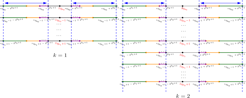
Hereon, we provide a general overview on our proof of Theorem 3.1, which encapsulates the primary challenge. Initially, for a fixed unit flow from to passing through , we label points where the unit flow enters as . Here represents a random variable taking values on (see specific definitions in the final part of this subsection). The area surrounding these points is segmented into intervals of length for , which we will refer to as the -th layer intervals.
First, we say an interval is very good if any unit flow must traverse it and generate substantial energy within it (see Definition 3.4). In search of very good intervals, we will investigate intervals in different layers step by step. The exact number of layers in each step is determined by a sequence (see (3.7)), whose definition includes two parameters and to facilitate our adjustments later. Using the estimate for the number of good intervals in Proposition 2.2, it can be inferred that with high probability we can find at least one very good pair of intervals near every inflow point in each step, as incorporated in Proposition 3.6. This event will be defined as in Definition 3.5 below.
Next, a recursive formula for the -quantiles of the effective resistances will be established in Subsection 3.2. To arrive at this, we will show that on the event (here is an event to ensure that is not close to the point , see Lemma 3.12), any flow must pass through many very good intervals, each of which provides sufficiently large energy and thus result in a significant contribution to the effective resistance. This will allow us to obtain an effective lower bound for the resistance (see Lemma 3.13). Thus by appropriately selecting parameters and , we can establish the recursive formula for the -quantiles in Proposition 3.11.
After that, we will establish an exponential lower bound for the -quantile from the recursive formula in Proposition 3.11. Combining this with appropriately selecting parameters and , we will complete the proof of Theorem 3.1. This is included in Subsection 3.3.
In the final of this part, we will introduce some notations which will be used repeatedly. Fix a sufficiently large and recall that . For convenience, let denote the set of all edges with one endpoint in the interval and the other endpoint in , and denote as the collection of those endpoints in . Formally,
| (3.3) |
Clearly, since . Additionally, for , let denote the number of points in . More specifically, for , denote
| (3.4) |
Then can be expressed as
According to the independence of edges, it follows that are independent random variables with expectations
for . By a simple calculation, we can see that there exists a constant (depending only on ) such that
| (3.5) |
We also denote . It is clear that
We now sort points in in the ascending order and denote them as .
Denote
| (3.6) |
Write for the sequence satisfying
| (3.7) |
where and are two constants which will be determined later (see (3.24) and (3.25) below). Note that is dependent on , but for the sake of brevity, the notation we are using here does not reflect this. We also define
| (3.8) |
and
| (3.9) |
3.1. Very good intervals and associated estimates
We begin by extending the definition of to a more general definition of effective resistance produced by unit flows passing through an interval. Specifically, for two intervals and with , define
| (3.10) | ||||
We will refer to as the effective resistance generated by unit flows (confined to ) passing through the interval . Moreover, from (3.1) and (3.10), it is obvious that . The definitions of and imply that
In particular, when , we have .
It is worth emphasizing that if we remove the edge set from the -LRP model and view it as a new graph, then becomes the classical effective resistance on this new graph. Thus, clearly possesses the fundamental properties of the effective resistance, as presented in the following lemma.
Lemma 3.3.
For any two intervals with , we have
-
(1)
;
-
(2)
for all intervals .
Proof.
Recall that is defined in (3.3). We now introduce the definition of “very good” intervals as follows.
Definition 3.4.
Fix . For and , we say the pair of intervals is -very good if
-
(1)
and are not directly connected by any long edge, as well as and are not directly connected by any long edge;
-
(2)
the resistance ;
-
(3)
the resistance .
It is worth emphasizing that the event in (1) is a modified version of the definition of good pair of intervals in Definition 2.1. Indeed, it can be observed that the event in Definition 3.4 (1) contains the event . This implies
| (3.11) |
We use the event in Definition 3.4 (1) here because the effective resistance (see (3.1)) we mainly consider in this section does not depend on whether the intervals contained in are good. Specifically, the interval serves as the outflow region for flows in the definition of , preventing them from re-entering.
In addition, it is clear that the event in Definition 3.4 (2) (resp. (3)) depends only on those edges with at least one endpoint falling within the interval (resp. ), while the event in Definition 3.4 (1) depends only on the edge set
Thus given , the events in Definition 3.4 (1), (2) and (3) are independent. Moreover, recall that represents the -quantile of defined in (3.2). Then from Lemma 3.3 (2) and the translation invariance of the model, we have
| (3.12) | ||||
For the sake of concise notation, we write
| (3.13) |
We next define the following event.
Definition 3.5.
For and , let be the event that the following conditions hold.
-
(1)
For each , .
-
(2)
For each and each , there exists at least one -very good pair of intervals in .
The main result of this subsection provides the following estimate for .
Proposition 3.6.
For any , there exist large enough (depending only on ), and (depending only on and ) such that for all and all , we have .
In what follows, we fix . To simplify notation, we will use to represent . Since the probability of the event is challenging to estimate directly, we will decompose it further as follows.
Definition 3.7.
For each and each , let be the event that none of pairs of intervals , is -very good.
Then from the definition of in Definition 3.5, we can see that
| (3.14) |
We now provide an upper bound for .
Lemma 3.8.
There exists a constant depending only on such that for each and each , we have
Proof.
For each and each , we let be the event that there exist at least pairs of intervals in such that the event in Definition 3.4 (1) occurs. Here is the constant in Proposition 2.2, depending only on . Note that the event is determined by the edge set and the position of from the Definition 3.4 (1). Moreover, the position of is determined by , which is independent of . Thus, from Proposition 2.2 and (3.11) we get that
By taking expectations on both sides of the above inequality, we obtain
| (3.15) |
In addition, for each , we denote for the event that , and denote . It is clear that is the event in Definition 3.5 (1).
According to the Chernoff bound, we have the following estimate.
Lemma 3.9.
For each ,
Therefore,
| (3.16) |
Proof.
To prove Proposition 3.6, we also need some asymptotic properties of the sequence . To this end, we define for . That is,
| (3.17) |
Lemma 3.10.
Let and . For the sequence , we have
| (3.18) |
Proof.
From (3.17), we can see that is increasing and is just determined by and . We will establish (3.18) by an induction on .
With the above lemmas at hand, we can present the
Proof of Proposition 3.6.
From (3.14), (3.16) and Lemma 3.8, we arrive at
| (3.21) | ||||
In addition, it follows from (3.20) and (3.5) that there exist two constants (depending only on ) such that for each ,
| (3.22) |
This implies
| (3.23) |
for some constant depending only on . Applying (3.20), (3.22) and (3.23) to (3.21), we conclude that
where are some constants depending only on . We now take large enough such that
| (3.24) |
It is worth emphasizing that constants and depend only on , meaning that also depends only on . Then we get
| (3.25) |
for some constants depending only on . Hence we complete the proof by taking and sufficiently large . ∎
3.2. A recursive formula of the -quantile
Recall that for and , represents the effective resistance defined in (3.1), and defined in (3.2) represents the -quantile of . The following proposition is the main output of this subsection, which gives a recursive relation for the sequence .
Proposition 3.11.
For any , there exists a constant depending only on such that the following holds for all . There exist large enough (depending only on ), and (depending only on and ) such that for all ,
where is defined in (3.17).
The proof of Proposition 3.11 will be presented at the end of this subsection. Before that, we make some preparations. Let us start by controlling the position of , which will help us determine which will satisfy that .
Lemma 3.12.
For any , there exist constants and (both depending only on and ) such that for all ,
We will refer to the event as .
Proof.
By the definitions of and in (3.4), we can see that
Hence, for fixed , we can complete the proof by taking and . ∎
Define
| (3.26) | ||||
where is the constant in Lemma 3.12. It can be observed that depends only on and , and the definition of it ensures that on the event we have
The key input of the proof of Proposition 3.11 is to show that on the event , the effective resistance is bounded from below by as follows.
Lemma 3.13.
To prove Lemma 3.13, we recall that is the set defined in (3.3). Let denote a unit flow that satisfies conditions specified in (3.1), i.e., is a unit flow from to with for all . For notation convenience, for , let denote the portion of the flow that passes through the point . Therefore, is a flow that enters the interval starting from the point (see Figure 6). More precisely, we can decompose the flow into self-avoiding paths using the algorithm in [8, Page 54], and thus obtain a sequence of flows . Then we can see that
Here means that lies on the path . It can be observed from the algorithm that exhibit unidirectionality, i.e.
| (3.27) |
and
| (3.28) |
Here, refers to the amount of the flow as defined in (1.10).

For each , consider the point , where . Indeed, by the definition of in (3.8), we have
We also define as the number such that is an -very good pair of intervals. If there are multiple such numbers, we take to be the smallest one. It is worth emphasizing that is well defined on the event . Additionally, for any flow and any interval , let us define as the portion of the flow that passes through . That is,
| (3.29) |
For , we also write for the portion of flows that pass through , i.e.,
| (3.30) |
Lemma 3.14.
Assume that the event occurs and recall is the constant defined in (3.26) with . Then for each ,
Proof.
Assume that occurs and fix . For notation convenience, we will denote as throughout the proof. By Definition 3.4 (1) for the -very good pair of intervals, we can see that on the event , we have
-
(1)
and are not directly connected by any long edge;
-
(2)
and are not directly connected by any long edge.
Moreover, since and , it is clear that
| (3.31) |
In addition, by definitions of and in (3.26), we have that
which implies for all . Combining this with (3.31) and (1), we conclude that every flow, departing from the interval to , must pass through the interval . This implies that the flow passes through for all . Similarly, from (1) and again, we can also see that the flow (from to ) must pass through the interval (see Figure 7 for an illustration). Therefore, combining this with the definition of in (3.30), we can obtain the desired result. ∎

In the following, we will use the -th layer pairs of intervals to represent for . For each , we want to establish a lower bound for the amount of flows passing through the pairs of intervals from the -th to the -th layers.
For fixed , let us start by extending the definition of to general . For each , let us define as the number such that is an -very good pair of intervals. If there are multiple such numbers, we select the smallest one for . Additionally, it is important to emphasize that when , the -very good pair of intervals chosen here corresponds to , which is defined in the paragraph below (3.28).
We show that flows passing through those -very good pairs of intervals , are significant as follows.
Lemma 3.15.
For any fixed , we have
Proof.
We also need the following lemma.
Lemma 3.16.
Assume that with . If or , then we have .
Proof.
We will prove the case when here, and the other cases can be proved similarly. Given that , from for all we have
| (3.32) |
We now turn to the
Proof of Lemma 3.13.
For a fixed , recall that we have assumed that the event occurs, is the constant defined in (3.26) with , and represents the -quantile of the effective resistance (see (3.2)).
For each , since the event in Definition 3.5 (1) for occurs, from (3.13) and (3.5) we can see that there is a constant (depending only on ) such that
Combining this with Lemma 3.15 and the definition of -very good pair of intervals in Definition 3.4 (2) and (3), we get that the sum of energies (i.e. effective resistance) of flows passing through the pairs of intervals from the -th to the -th layers is at least
| (3.33) | ||||
We next consider the total energy generated by flows passing through all layers from to . It follows from Lemma 3.16 that although intervals from different layers may intersect, any two intersecting intervals must have different subscripts . This implies that for intersecting intervals, the energy considered in different layers comes from energies generated by different flows (see Figure 8 for an illustration). Therefore, by (3.27) we can add up the above energy of each layer and get a lower bound
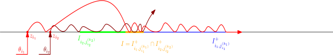
| (3.34) |
(See Figure 9 for an illustration). Hence we complete the proof by taking , which depends only on . ∎
We now can provide the
Proof of Proposition 3.11.
Fix . Throughout the proof, we also fix a sufficiently large satisfying (3.24), which depends only on .
According to (3.26) and the definition of in (3.7), there exists a constant (depending only on and ) such that for all , we have In addition, by taking in Proposition 3.6, we get that there exist and such that when , we have for all . Combining the above analysis with Lemma 3.12, we can see that for and for all ,
Applying this into Lemma 3.13 we arrive at
for some constant depending only on . Therefore, by the definition of -quantile of in (3.2), we see that
for all . ∎
3.3. Proof of Theorem 3.1 and Proposition 3.2
Let us start with the
Proof of Proposition 3.2.
Fix . Recall that Proposition 3.11 gives a recursive formula for -quantiles . With the choice of (depending only on ) and (depending only on and ) as in Proposition 3.11, from Lemma 3.10 we can see that there exists (depending only on and ) such that
| (3.35) |
We also choose (depending only on and ) such that , and choose (depending only on and ) such that
| (3.36) |
We now turn to the
Proof of Theorem 3.1.
Fix . We begin by considering the event . From Proposition 3.6, we obtain that there exist large enough (depending only on ), and (both depending only on and ) such that when , we have for all .
We next turn to the event . It follows from Lemma 3.12 that there exist and (both depending only on and ) such that for all , we have . Moreover, according to (3.26) and the definition of in (3.7), we can see that there exists a constant (depending only on and ) such that for all , we have
We now apply and satisfying (3.24) to the definition of in (3.7). Then combining this with , Lemma 3.13 and Proposition 3.2, we can see that on the event ,
where and are parameters in Proposition 3.2 with (depending only on ), and are positive constants (both depending only on and ). Therefore, from the above analysis we can find (depending only on and ) such that
Furthermore, since and depend only on and , we can take (depending only on and ) such that
Hence, the proof is complete. ∎
4. Proof of Theorem 1.1
For , we recall that is the effective resistance between and as defined in (1.2) with and , and that is the effective resistance generated by unit flows from to , passing through the interval as defined in (1.7). In particular, recall that since .
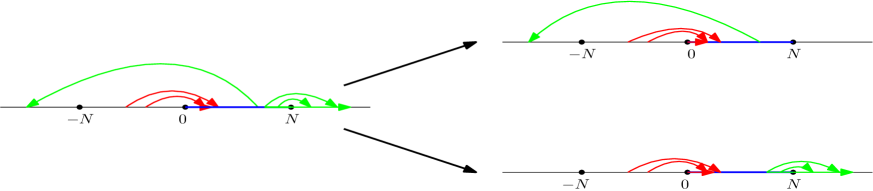
As we mentioned in Subsection 1.2, to complete the proof of Theorem 1.1, it is essential to establish a lower bound on in terms of , which will allow us to use estimates for in Section 3. To achieve this, note that flows in the definition of will eventually flow into (either of) the two intervals and . Therefore, we further decompose (see Figure 10) and define
| (4.1) | ||||
as the effective resistance generated by unit flows from to , passing through the interval . Note that if there is no edge joining and , we have .
4.1. Properties of
In this subsection, our goal is to show the existence of a certain stochastic control between and (see (4.4) below). This will allow us to obtain that with high probability, also exhibits an exponential lower bound from estimates for in Section 3.
Now for any , , and any , it is obvious that
| (4.2) | ||||
In addition, assume that is given. According to the monotonicity property of the effective resistance in Lemma 3.3 (2), we have that is non-increasing with respect to the edge set connecting and . That is, for any two deterministic edge sets with ,
| (4.3) |
where represent effective resistances as defined in (3.10) by replacing by , respectively.
From the above analysis, we claim that for any ,
| (4.4) |
Indeed, the second inequality can be obtained from the monotonicity property of the effective resistance in Lemma 3.3 (2). For the first inequality in (4.4), let
From (4.2), we can construct a coupling of such that
and . Then combining this with (4.3), we arrive at
where and are effective resistances as defined in (3.10) by replacing by and , respectively. This implies the first inequality in (4.4).
Lemma 4.1.
For any , there is a constant (depending only on ) such that the following holds. For any , there exists a constant (depending only on and ) such that for all ,
Furthermore, we have the following estimate for .
Lemma 4.2.
For any , there is a constant (depending only on ) such that the following holds. For any , there exists a constant (depending only on and ) such that for all ,
Proof.
let for some . From Theorem 3.1 and Lemma 4.1, there exists a constant (depending only on ) such that the following holds. For any , there exists a constant (depending only on and ) such that for all ,
| (4.5) |
Now assume that the event occurs. Let be the unit flow from to , passing through the interval , such that
Denote and as portions of flow which enters intervals and , respectively. Then
Clearly, . In particular, if there is no edge joining and , then .
4.2. Proof of Theorem 1.1
The proof of Theorem 1.1 is divided into proofs of (1.3) and (1.4). Since there are similarities between the two proofs, we will omit some details of the similar parts in the proof of (1.4). Let us start by the
Proof of (1.3) in Theorem 1.1.
We begin by considering the case for some . According to the translation invariance of the model, we can see that and have the same distribution. Therefore, from Lemma 4.2, there exists a constant (depending only on ) such that the following holds. For any , there exists a constant (depending only on and ) such that for all ,
| (4.6) |
Now assume that the event occurs. Let be the unit flow from 0 to that minimizes the right-hand side of (1.2), that is,
Since must flow into finally, it must pass through either or . In light of this, let be the portion of flow that passes through the interval and then flow into . Similarly, we define by replacing with in the definition of . Then we have (see (1.6) for more details). Combining this with the definition of the effective resistance in (1.7), we get that on the event ,
| (4.7) | ||||
Here is a constant depending only on and , and is a constant depending only on . Hence, from (4.6) and (4.7) we can conclude
| (4.8) |
For general , let such that with . Since the effective resistance is nondecreasing with , we have
Therefore, for any , by (4.8) we obtain that
where is a constant depending only on and . Hence, the proof is complete. ∎
We next turn to the effective resistance . We also first consider the case for some . Similar to (4.1), we define
as the effective resistance generated by unit flows from to , passing through the interval . Note that if there is no edge joining and , we then have . Using similar arguments for (4.4) and the translation invariance of the model, we have that for all ,
Combining this with similar arguments in the proof of Lemma 4.2, we obtain the following estimate for , which is defined in (1.7) by replacing and with and , respectively.
Lemma 4.3.
For any , there is a constant (depending only on ) such that the following holds. For any , there exists a constant (depending only on and ) such that for all ,
We now can present the
Proof of (1.4) in Theorem 1.1.
Throughout the proof, we condition on , i.e., intervals and are not directly connected by any long edge.
We begin by considering the case for some . It is clear from the translation invariance of the model that and have the same distribution. Hence, from Lemma 4.3, there exists a constant (depending only on ) such that the following holds. For any , there exists a constant (depending only on and ) such that for all ,
| (4.9) |
Note that, by the definition of , we can observe that the two effective resistances in (4.9) are both independent of the edge set . Therefore, (4.9) implies that
| (4.10) |
Now assume that the event occurs. Let be the unit flow from to such that
Similar to the argument in the proof of (1.3), we can define as the portion of flow that passes through the interval and then flow into , and define by replacing with in the definition of . Then we also have . Therefore, we get that on the event ,
Here is a constant depending only on and , and is a constant depending only on . Hence, combining this with (4.10), we can conclude
For general , we can complete the proof by using the similar argument in the proof of (1.3). ∎
Acknowledgement. We warmly thank Jian Wang for stimulating discussions at an early stage of the project. L.-J. Huang would like to thank School of Mathematical Sciences, Peking University for their hospitality during her visit. J. Ding is partially supported by NSFC Key Program Project No. 12231002 and the Xplorer prize. L.-J. Huang is partially supported by National Key R&D Program of China No. 2023YFA1010400.
References
- [1] D.-J. Aldous and J.-A. Fill. Reversible Markov chains and random walks on graphs. 2002. URL www.berkeley.edu/users/aldous/book.html.
- [2] P. Alessandro and S. Aravind. Randomized distributed edge coloring via an extension of the Chernoff-Hoeffding bounds. SIAM J. Comput., 26(2):350–368, 1997.
- [3] J. Bäumler. Distances in percolation models for all dimensions. Comm. Math. Phys., page 1–76, 2023.
- [4] I. Benjamini, N. Berger, and A. Yadin. Long-range percolation mixing time. Combin. Probab. Comput., 17(4):487–494, 2008.
- [5] N. Berger. Transience, recurrence and critical behavior for long-range percolation. Comm. Math. Phys., 226(3):531–558, 2002.
- [6] N. Berger and Y. Tokushige. Scaling limits for random walks on long range percolation clusters. arXiv:2403.18532, 2024.
- [7] M. Biskup, X. Chen, T. Kumagai, and J. Wang. Quenched invariance principle for a class of random conductance models with long-range jumps. Probab. Theory Related Fields, 180(3-4):847–889, 2021.
- [8] M. Biskup, J. Ding, and S. Goswami. Return probability and recurrence for the random walk driven by two-dimensional gaussian free field. Commun. Math. Phys., 373:45–106, 2020.
- [9] V.H. Can, D.A. Croydon, and T. Kumagai. Spectral dimension of simple random walk on a long-range percolation cluster. Electron. J. Probab., 27(56):37, 2022.
- [10] X. Chen, T. Kumagai, and J. Wang. Quenched local limit theorem for random conductance models with long-range jumps. arXiv:2402.07212, 2024.
- [11] N. Crawford and A. Sly. Simple random walk on long range percolation clusters I: heat kernel bounds. Probab. Theory Related Fields, 154(3):753–786, 2012.
- [12] N. Crawford and A. Sly. Simple random walk on long-range percolation clusters II: scaling limits. Ann. Probab., 41(2):445–502, 2013.
- [13] P.G. Doyle and J.L. Snell. Random Walks and Electric Networks. Carus Mathematical Monographs 22. Mathematical Association of America, Washington, DC, 1984.
- [14] S. Gallo, N.L. Garcia, V.V. Junior, and P.M. Rodríguez. Rumor processes on and discrete renewal processes. J. Stat. Phys, 155:591–602, 2014.
- [15] T. Kumagai. Random Walks on Disordered Media and Their Scaling Limits. École d’Été de Probabilités de Saint-Flour XL-2010. Lecture Nots in Mathematics 2101. Springer, Cham, 2014.
- [16] T. Kumagai and J. Misumi. Heat kernel estimates for strongly recurrent random walk on random media. J. Theor. Probab., 21:910–935, 2008.
- [17] D.A. Levin, Y. Peres, and E.L. Wilmer. Markov Chains and Mixing Times. Amer. Math. Soc., Providence, RI, 2009. With a chapter by J.G. Propp and D.B. Wilson.
- [18] R. Lyons and Y. Peres. Probability on Trees and Networks. Cambridge Univ. Press, Cambridge, 2006.
- [19] J. Misumi. Estimates on the effective resistance in a long-range percolation on . J. Math. Kyoto Univ., 48(2):389–400, 2008.
- [20] I. Russell and K. Valentine. Constructive proofs of concentration bounds. Approximation, randomization, and combinatorial optimization, pages 617–631, 2010.
- [21] L.S. Schulman. Long-range percolation in one dimension. J. Phys. A, 16(17):L639–L641, 1983.
- [22] Z.Q. Zhang, F.C. Pu, and B.Z. Li. Long-range percolation in one dimension. Journal of Physics A: Mathematical and General, 16(3):L85, 1983.